Identification of Location and Camera Parameters for Public Live Streaming Web Cameras

Abstract

Public live streaming web cameras are quite common now and widely used by drivers for qualitative analysis of traffic conditions. At the same time, they can be a valuable source of quantitative information on transport flows and speed for the development of urban traffic models. However, to obtain reliable data from raw video streams, it is necessary to preprocess them, considering the camera location and parameters without direct access to the camera. Here we suggest a procedure for estimating camera parameters, which allows us to determine pixel coordinates for a point cloud in the camera’s view field and transform them into metric data. They are used with advanced moving object detection and tracking for measurements.

1. Introduction

There are many ways to measure traffic [1,2,3]. The most common in the practice of road services are radars combined with video cameras and other sensors. The measuring complexes are above or at the edge of the road. Inductive sensors are the least dependent on weather conditions and lighting. The listed surveillance tools assume installation by the road or on the road. Providers of mobile navigator applications receive data about the car’s movement from the sensors of mobile devices. Autonomous cars collect environmental information using various sensors, including multiview cameras, lidars, and radars. The results of the data collection systems of road services, operators of navigators, and autonomous cars are usually not available to third-party researchers. Notably, pioneering traffic analysis work describes processing video data recorded on film [3] (pp. 3–10).

Operators worldwide install public web cameras, many of which look at city highways; e.g., there are more than a hundred similar cameras available in Vladivostok.

A transport model verification requires actual and accurate data on transport traffic, covering a wide range of time intervals with substantial transport activity. Public live-streaming cameras can be a good and easily accessible source of data for that kind of research. Of course, this accessibility is relative. Video processing involves storing and processing large amounts of data.

The ref. [4] demonstrates road traffic statistics collection from a public camera video, where the camera has little perspective and radial distortions in the region of interest in the road (Region Of Interest, ROI). However, the distortions make significant changes in images for the majority of public cameras. The current article generalizes this approach to the case where a camera has essential radial and perspective distortions.

Street camera owners usually do not announce camera parameters (focal length, radial distortion coefficients, camera position, orientation). Standard calibration procedures with a pattern rotation can be useless for cameras on a wall or tower. In this case, we suggest the implementable camera calibration procedure, which uses only online data (global coordinates of some visible points, photos, and street view images).

With known camera parameters, we construct the mapping between the ROI pixel coordinates and metric coordinates of points on the driving surface, which gives a way to estimate traffic flow parameters in standard units such as car/meter for traffic density and meter/second for car velocity with improved accuracy.

2. Coordinate Systems, Models

We select an ENU coordinate frame $F_{enu}$ (East, North, Up) with an origin on a fixed object to localize points $P=(x_e,y_e,z_e)$, where $x_e,y_e,$ and $z_e$ are coordinates of P in $F_{enu}$.

A camera forms an image in the sensor (Figure 1 and Figure 2). A digital image is a pixel matrix $N\times M$ (N columns, M rows). A pixel position is described in the image coordinate frame $F_{im}$ in the image plane $P_{im}=(u,v)$ where u and v are real numbers, coordinates of $P_{im}$ in $F_{im}$. Axis U corresponds to the image matrix rows (towards the right), and axis V corresponds to columns (from up to down). The camera orientation determines the image sensor plane orientation. Integer indexes define pixel position in the image matrix. We can obtain them by rounding u and v to the nearest integers. Let w and h be the image pixel width and height, respectively. For the image width and height, we have $W=Nw$ and $H=Mh$.

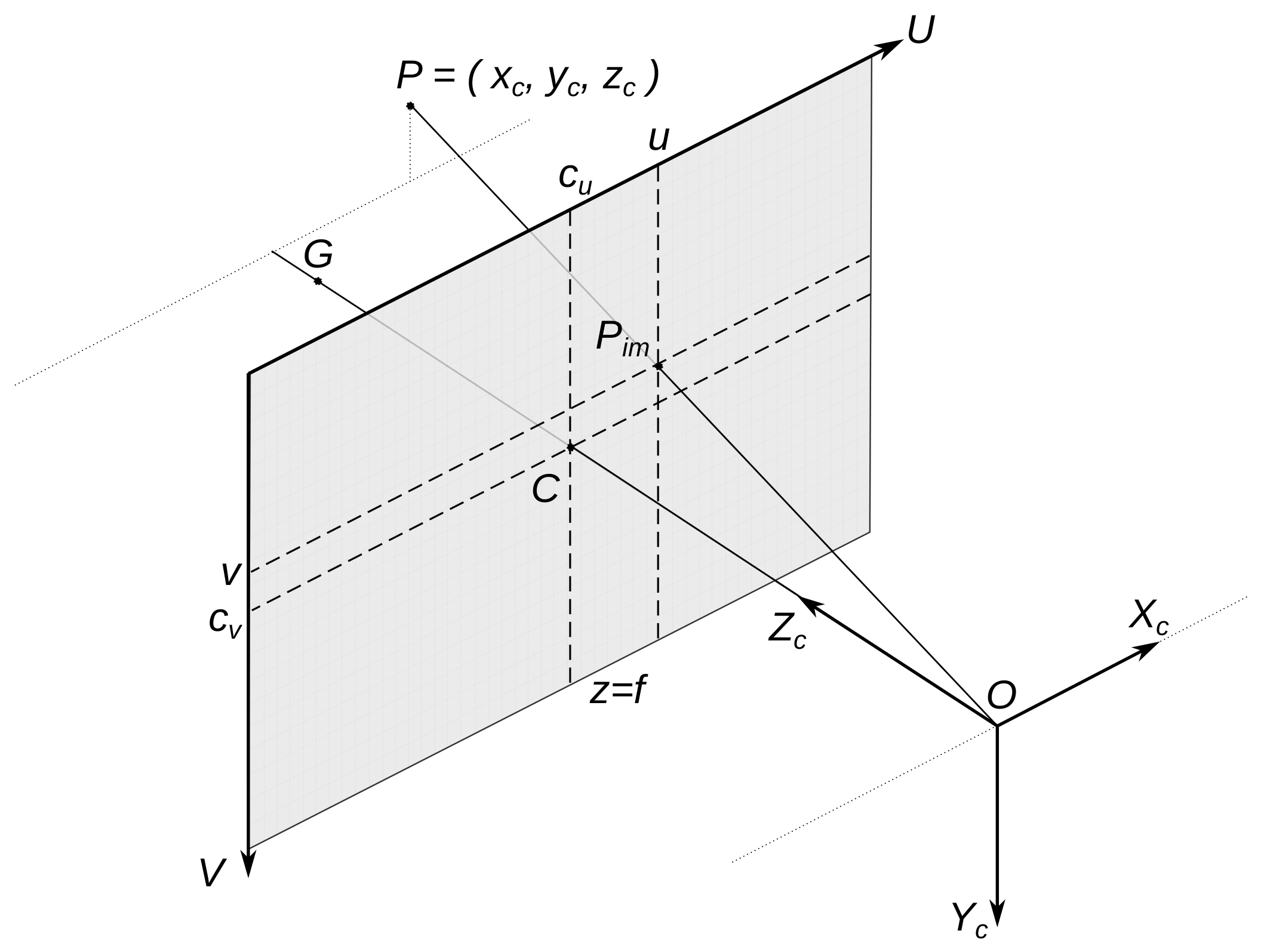
Camera position and orientation define the camera coordinate frame $F_c$ (Figure 1). The camera perspective projection center O is the origin of $F_c$. We denote by $(O_{xe},O_{ye},O_{ze})$ the O coordinates in $F_{enu}$. Axis $Z_c$ follows along the camera optical axis, axis $X_c$ is parallel to axis U, and $Y_c$ is parallel to axis V. Axis $X_c$ defines the camera horizon. The deviation of $X_c$ from the horizontal plane $X_{enu}{Y}_{enu}$ defines the camera horizon tilt. Unlike $F_{im}$, the $F_{enu}$ and $F_c$ are metric coordinate frames. $F_{im}$ coordinates $(u,v)$ approximate matrix indexes. To obtain meters from u on axis U, we use the expression $m\left(u\right)=wu$, and to obtain meters from v on axis V, we use $m\left(v\right)=hv$.

Suppose the camera builds an image close to a perspective projection of a 3D scene. We describe this camera transformation as the pinhole camera model (Figure 1, Figure 2 and ref. [5]). A point image $P_{im}=(u,v)$ is the transformation of the original 3D point P coordinates described in $F_{enu}$. The matrices A and $\left[R\right|t]$ define this transformation:

$$A=\left[\begin{array}{ccc}{f}_u& 0& c_u\\ 0& f_v& c_v\\ 0& 0& 1\end{array}\right],$$

(1)

$$\left[R\right|t]=\left[\begin{array}{cccc}{r}_{11}& r_{12}& r_{13}& t_x\\ r_{21}& r_{22}& r_{23}& t_y\\ r_{31}& r_{32}& r_{33}& t_z\end{array}\right].$$

(2)

The triangular matrix A contains the intrinsic parameters of the camera. Camera position and orientation determine matrix $\left[R\right|t]$. Matrix $\left[R\right|t]$ defines transformation from frame $F_{enu}$ to camera coordinates $F_c$:

$$\left[\begin{array}{c}{x}_c\\ y_c\\ z_c\end{array}\right]=\left[R\right|t]\left[\begin{array}{c}{x}_e\\ y_e\\ z_e\\ 1\end{array}\right], \left[\begin{array}{c}{t}_x\\ t_y\\ t_z\end{array}\right]=-R\left[\begin{array}{c}{O}_{xe}\\ O_{ye}\\ o_{ze}\end{array}\right].$$

(3)

Here, R is a rotation matrix, and t is the shift vector from the origin of $F_{enu}$ to O (origin of $F_c$). Matrix A includes the principal point C coordinates $(c_u,c_v)$ in frame $F_{im}$ and the camera focal length f divided by pixel width and height:

$$f_u=f/w, f_v=f/h.$$

(4)

The camera’s optical axis and the image plane intersect at C. It is the spatial point G image (Figure 1 and Figure 2). Usually, the coordinates $(c_u,c_v)$ point to the image sensor matrix center (e.g., full HD resolution is 1920 × 1080, so $c_u=960,c_v=540$). Some modes of cameras can produce cropped images shifted from the principal point; we do not consider this case here.

The triangles $(O,P_{im},C)$ and $(O,P,(z_c,0,0))$ are similar on the plane $Z{X}_c$ and on $Z{Y}_c$ (Figure 2), so

$$\begin{array}{c}{x}_c/z_c=w(u-c_u)/f=tan{\theta }_x\\ y_c/z_c=h(v-c_v)/f=tan{\theta }_y\end{array}.$$

(5)

It follows from (5) that pixel coordinates in $F_{im}$ are connected with coordinates of the spatial source in $F_c$ by the equations

$$P_{im}^h=\left[\begin{array}{c}u\\ v\\ 1\end{array}\right]=A\left[\begin{array}{c}{x}_c/z_c\\ y_c/z_c\\ 1\end{array}\right]=\left[\begin{array}{c}{f}_u{x}_c/z_c+c_u\\ f_v{y}_c/z_c+c_v\\ 1\end{array}\right],$$

(6)

where $P_{im}^h$ are homogeneous coordinates of $P_{im}$. If $f_u\ne 0$ and $f_v\ne 0$, the pixel $(u,v)$ defines the relations $x_c/z_c,y_c/z_c$ (5). However, we need to know the value $z_c(u,v)$ (“depth map”) to recover original 3D coordinates $x_x,y_c,$ and $z_c$ from the pixel coordinates $(u,v)$. Additional information about the scene is needed to build the depth map $z_c(u,v)$ for some range of pixels $(u,v)$. Perspective projection preserves straight lines.

A wide-angle lens, used by most street public cameras, introduces perspective distortion described by the pinhole camera model and substantial radial distortion. Usually, the radial distortion is easily detectable, especially on ”straight” lines near the edges of the image. An extended model was used to take it into account. A popular quadratic model of radial distortion ([6] (pp. 63–66), [7] (pp. 189–193), [5]) changes the pinhole camera model (6) as follows:

$$r^2={(x_c/z_c)}^2+{(y_c/z_c)}^2,$$

(7)

$$\left[\begin{array}{c}\widehat{x}\\ \widehat{y}\end{array}\right]=(1+k_1{r}^2+k_2{r}^4)\left[\begin{array}{c}{x}_c/z_c\\ y_c/z_c\end{array}\right],$$

(8)

$$P_{im}^h=\left[\begin{array}{c}u\\ v\\ 1\end{array}\right]=A\left[\begin{array}{c}\widehat{x}\\ \widehat{y}\\ 1\end{array}\right]=\left[\begin{array}{c}{f}_u\widehat{x}+c_u\\ f_v\widehat{y}+c_v\\ 1\end{array}\right],$$

(9)

where $k_1$ and $k_2$ are radial distortion coefficients. In addition to the quadratic, more complex polynomials and models of other types are used ([5], [6] (pp. 63–66, 691–692), [7] (pp. 189–193)). Let the coefficients $f_u,f_v,c_u,c_v,k_1,$ and $k_2$ be selected so that the formation of images from the camera is sufficiently well described by (7)–(9). To construct the artificial image on which the radial distortion $k_1$ and $k_2$ is eliminated, we must for each pair of relations $(x_c/z_c,y_c/z_c)$ obtain new positions of pixels $(\widehat{u},\widehat{v})$ according to the pinhole camera model:

$$\left[\begin{array}{c}\widehat{u}\\ \widehat{v}\end{array}\right]=\left[\begin{array}{c}{f}_u{x}_c/z_c+c_u\\ f_v{y}_c/z_c+c_v\end{array}\right].$$

(10)

To do this, we need all values $(x_c/z_c,y_c/z_c)$ (coordinates in $F_c$), which form the original image. To obtain the relations from an image, you have the image pixel coordinates $(u,v)$ and equations (follows from (7)–(9))

$$Q(u,v)=\frac{f_v(u-c_u)}{f_u(v-c_v)}, D(u,v)=Q^2+1,$$

(11)

$$x_c/z_c=Q(u,v)y_c/z_c,$$

(12)

$$k_{2}D{(u,v)}^2{(y_c/z_c)}^5+k_{1}D(u,v){(y_c/z_c)}^3+y_c/z_c+\frac{c_v-v}{f_v}=0,$$

(13)

if $v\ne c_v$. Similar equations are valid for $v=c_v$ and $u\ne c_u$. Equation (13) has five roots (complex, generally speaking), so we need an additional condition to select one root. We can select the real root nearest to $(v-c_v)/f_v$. The artificial image will not be a rectangle, but we can select a rectangle part of it (see figures of Example 2). Note that the mapping $(u,v)\to (\widehat{u},\widehat{v})$ is determined by the camera parameters $f_u,f_v,c_u,c_v,k_1,$ and $k_2$. It does not change from frame to frame and can be computed once and used before the parameters are changed.

3. Public Camera Parameters Estimation

Model parameters (3), (7)–(9) define the transformation of the 3D point, visible by camera, to pixel coordinates in the image. These parameters are: rotation matrix of the camera orientation R (2) and (3); camera position coordinates (point O) in $F_{enu}$ (3); intrinsic camera parameters $f_u,f_v,c_u,$ and $c_v$, (1) and (4); and radial distortion coefficients $k_1$ and $k_2$, (8) and (9).

The camera calibration process estimates the parameters using a set of 3D point coordinates $\left\{P_{enu}^i\right\}$ and a set of the point image coordinates $\left\{P_{im}^i\right\}$. The large set $\left\{P_{enu}^i\right\}$ is called a point cloud. There are software libraries that work with point clouds. Long range 3D lidars or geodesic instruments measure 3D coordinates values for a set $\left\{P_{enu}^i\right\}$. Another camera depth map can help obtain a set $\left\{P_{enu}^i\right\}$. Stereo/multi-view cameras can build depth maps, but it is hard to obtain high accuracy for long distances. When the tools listed above are unavailable, it is possible to obtain global coordinates of points in the camera field of view by GNSS sensors or from online maps. The latter variants are easier to access but less accurate. There are many tools [8] to translate global coordinates to an ENU.

Camera calibration procedure is well studied ([7] (pp. 178–194), [9] (pp. 22–28), [10], [6] (pp. 685–692)). It looks for the parameter values that minimize the difference between pixels $\left\{P_{im}^i\right\}$ and pixels generated by the model (3), (7)–(9) from $\left\{P_{enu}^i\right\}$. Computer vision software libraries include calibration functions for a suitable set of images from a camera [5]. The OpenCV function calibrateCamera [5,11] needs a set of points and pixels of a special pattern (e.g., “chessboard”) rotated before the camera. The function returns an estimation of intrinsic camera parameters and camera placements concerning the pattern positions. These relative camera placements are usually useless after outdoor camera installation. If the camera uses a zoom lens and the zoom changes on the street, the camera focal length changes too, and new calibration is needed. If we use a public camera installed on a wall or tower, it is hard to collect appropriate pattern images from the camera to apply a function such as calibrateCamera. Camera operators usually do not publish camera parameters, but this information is indispensable for many computer vision algorithms. We need a calibration procedure applicable to the available online data.

Site-Specific Calibration

If the unified calibration procedure data are unavailable, we can estimate camera position and orientation parameters (R,O) separately from others. Resolution $N\times M$ of images/video from a camera is available with the images/video. As noted earlier, usually

$$c_u=N/2,c_v=M/2.$$

(14)

Many photo cameras (including phone cameras) add the EXIF metadata to the image file, which often contain focal length f. The image sensor model description can contain a pixel width w and height h, so (4) gives $f_u$ and $f_v$ values. The distortion coefficients are known for high-quality photo lenses. Moreover, the raw image processing programs can remove the lens radial distortion. If lucky, we can obtain intrinsic camera parameters and radial distortion coefficients and apply a pose computation algorithm (PnP, [12,13]) to sets $\left\{P_{enu}\right\}$, $\left\{P_{im}\right\}$ to obtain R,O estimates. When EXIF metadata from the camera are of no help (this is typical for most public cameras), small sets $\left\{P_{enu}\right\}$ and $\left\{P_{im}\right\}$ and Equation (5) can help to obtain $f_u$ and $f_v$ estimations. Suppose we know the installation site of the camera (usually, the place is visible from the camera’s field of view). In that case, we can estimate GNSS/ENU coordinates of the place (point O coordinates) by the method listed earlier. The camera orientation (matrix R) can be detected with the point G coordinates (Figure 1) and the estimation of the camera horizon tilt. Horizontal or vertical 3D lines (which can be artificial) in the camera’s field of view can help evaluate the tilt.

4. Formulation of the Problem and Its Solution Algorithm

Designers and users of transport models are interested in the flow density (number of vehicles per unit of lane length or direction at a time); speed of vehicles (on a lane or direction); and intensity of the flow (number of vehicles crossing the cross section of a lane or direction). We capture some areas (ROI) of the frames to determine these values from a fixed camera. The camera generates a series of ROI images, usually at a fixed interval, such as 25 frames/second. The algorithms (object detection or instance segmentation or contours detection and object tracking, see [14,15,16,17]) find a set of contours describing the trajectory of each vehicle crossing the ROI. The contour description consists of the coordinates of the vertices in $F_{im}$. We count the number of contours per meter in the ROI of each frame to estimate flow density. We choose the vertex (e.g., “bottom left”) of the contour in the trajectory and count the meters that the vertex has passed in the trajectory to estimate the car speed. Both cases require estimation in meters of distance given in pixels, so we need to convert lengths in the image (in $F_{im}$) to lengths in space (in $F_{enu}$ or $F_c$). In some examples, distances in pixels are related to metric distances almost linearly (where radial and perspective distortions are negligible). We will consider the public cameras that produce images with significant radial and perspective distortions in the ROI (more common case).

Problem 1.

• Let Q be the area that is a plane section of the road surface in space (the road plane can be inclined);
• Φ is the camera frame of $N\times M$ resolution containing the image of Q, denoting the image by $Q_{im}$;
• The camera forms pixel coordinates of the image Φ according to the model (3), (7)–(9) with unknown parameters $f_u,f_v,k_1,k_2,R$,

  $$Q_{im}=\mathsf{\Lambda }\left(Q_{enu}\right);$$
• Φ contains the image of at least one segment, the prototype of which in space is a segment of a straight line with a known slope (e.g., vertical);
• The image is centered relative to the optical axis of the video camera, that is, $c_u=N/2$ and $c_v=M/2$;
• The $F_{enu}$ coordinates of the points O (camera position) and G (the source of the optical center C) are known;
• The $F_{im}$ coordinates of one or more pixels of $\{P_{im}^u\ne C\}$ located on the line $v=c_v$ and the $F_{enu}$ coordinates of their sources $\left\{P_{enu}^u\right\}$ are known;
• The $F_{im}$ coordinates of one or more pixels of $\{P_{im}^v\ne C\}$ located on the line $u=c_u$ and the $F_{enu}$ coordinates of their sources $\left\{P_{enu}^v\right\}$ are known;
• The $F_{enu}$ coordinates of three or more points $\left\{P_{enu}^Q\right\}\in Q$ are known; at least three of them must be non-collinear;
• The $F_{im}$ coordinates of one or more groups of three pixels $\left\{(P_{im}^a,P_{im}^b,P_{im}^c)\right\}$ are known, and in the group, the sources of the pixels are collinear in space.

Find the parameters of the camera $f_u,f_v,R,k_1,$ and $k_2$ and construct the mapping

$$Q_{enu}={\mathsf{\Lambda }}^{-1}\left(Q_{im}\right).$$

Online maps allow remote estimation of global coordinates of points and horizontal distances. Many such maps do not show the altitude, and most do not show the height of buildings, bridges, or vegetation. Online photographs, street view images, and horizontal distances can help estimate such objects’ heights. Camera locations are often visible in street photos. This variant of measurements suggests that the coordinate estimates may contain a significant error. The errors result in some algorithms (e.g., PnPransac) being able to generate a response with an unacceptable error.

To find $\left\{P_{im}^u\right\}$,$\left\{P_{enu}^u\right\}$,$\left\{P_{im}^v\right\}$, and $\left\{P_{enu}^v\right\}$ coordinates, the points must be visible both in the image and on the online map.

4.1. Solution Algorithm

We want to eliminate the radial distortion of area $Q_{im}$ to go to the pinhole camera model. From (10)–(13), it follows that for this you need values $f_u$ and $f_v$.

4.1.1. Obtain the Intrinsic Parameters (Matrix A)

Note that from $v^u=c_v$ and (7)–(9) it follows $yc/zc=0$ for the point $P_{im}^u=(u^u,v^u)$ (because $1+k_1{r}^2+k_2{r}^4=0$ leads to $u^u=c_u$ and $P_{im}^u=C$). So, the point $P_{im}^u$ stays on the central horizontal line of the image for any values $k_1$ and $k_2$. By analogy, for $P_{im}^v=(u^v,v^v)$ take place $x_c/z_c=0$, and the point stays on the central vertical line for any values $k_1$ and $k_2$.

Evaluate the angles between the optical axis $OG$ and vectors $O{P}_{enu}^u$ and $O{P}_{enu}^v$ (Figure 2, Figure 1):

$$\begin{array}{c}{\theta }_x=arccos(OG·O{P}_{enu}^u/\left(\right|OG\left|\right|O{P}_{enu}^u\left|\right))\\ {\theta }_y=arccos(OG·O{P}_{enu}^v/\left(\right|OG\left|\right|O{P}_{enu}^v\left|\right))\end{array}.$$

(15)

It follows from (5) that if the effect of radial distortion on the values $(u^u,v^u)$ and $(u^v,v^v)$ can be ignored (camera radial distortion is moderate, and the points are not too far from C), then

$$\begin{array}{c}{f}_u=(u^u-c_u)/tan{\theta }_x\\ f_v=(v^v-c_v)/tan{\theta }_y\end{array}.$$

(16)

Equation (16) gives the initial approximation of coefficients $f_u$ and $f_v$ and an evaluation of matrix A.

4.1.2. Obtain the Radial Distortion Compensation Map

Let $\widehat{\mathsf{\Phi }}$ be the image obtained from $\mathsf{\Phi }$ by the transformation (10) and solution of Equations (11)–(13). Denote $\mathsf{\Theta }$ the mapping of $\mathsf{\Phi }$ to $\widehat{\mathsf{\Phi }}$:

$$\widehat{\mathsf{\Phi }}=(\widehat{u},\widehat{v})=\mathsf{\Theta }(u,v;k_1,k_2,f_u,f_v,c_u,c_v)=(f_u{x}_c/z_c+c_u,f_v{y}_c/z_c+c_v).$$

(17)

We create the image $\widehat{\mathsf{\Phi }}$ according to the pinhole camera model. The model transforms a straight line in space into a straight line in the image.

Let $P_{im}^a=(u^a,v^a),P_{im}^b=(u^b,v^b),$ and $P_{im}^c=(u^c,v^c)$ in $F_{im}$ and

$${\widehat{P}}_{im}^a=({\widehat{u}}^a,{\widehat{v}}^a)=\mathsf{\Theta }(u^a,v^a),{\widehat{P}}_{im}^b=({\widehat{u}}^b,{\widehat{v}}^b)=\mathsf{\Theta }(u^b,v^b),{\widehat{P}}_{im}^c=({\widehat{u}}^c,{\widehat{v}}^c)=\mathsf{\Theta }(u^c,v^c).$$

(18)

We can find $k_1$ and $k_2$ values that minimize the sum of distances from pixels ${\widehat{P}}_{im}^b$ to the lines passing through ${\widehat{P}}_{im}^a$ and ${\widehat{P}}_{im}^c$. We calculate the distance as:

$$\frac{|({\widehat{u}}^c-{\widehat{u}}^a)({\widehat{v}}^a-{\widehat{v}}^b)-({\widehat{u}}^a-{\widehat{u}}^b)({\widehat{v}}^c-{\widehat{v}}^a)|}{\sqrt{{({\widehat{u}}^a-{\widehat{u}}^c)}^2+{({\widehat{v}}^a-{\widehat{v}}^c)}^2}}$$

(19)

for each triplet $(P_{im}^a,P_{im}^b,P_{im}^c)$. This approach is a variant of the one described, for example, in [7] (pp. 189–194). OpenCV offers the realization of ${\mathsf{\Theta }}^{-1}$ (initUndistortRectifyMap). It is fast, but we need to invert it for our case. We solve Equations (11)–(13) (including version for $v=c_v,u\ne c_u$) to obtain $\mathsf{\Theta }$. The ${\mathsf{\Theta }}^{-1}$ is polinomial from $\widehat{u},\widehat{v}$ (see (7)–(10)).

4.1.3. Obtain the Camera Orientation (Matrix R )

To determine the camera orientation, we use the point O and the point G given in the coordinates $F_{enu}$ (Figure 1). Unit vector

$${\overrightarrow{\mathbf{e}}}_{zc}=OG/\left|OG\right|={(e_x^{zc},e_y^{zc},e_z^{zc})}_{enu}$$

(20)

gives direction to axis $Z_c$ of frame $F_c$. ${\overrightarrow{\mathbf{e}}}_{zc}$, and O determines the plane of points x, for which the vector $\overrightarrow{O}$ is perpendicular to ${\overrightarrow{\mathbf{e}}}_{zc}$. In this plane, lie the axes $X_c$ and $Y_c$ of coordinate frame $F_c$. Unit vector ${\overrightarrow{\mathbf{e}}}_d={(0,0,-1)}_{enu}$ is downward. Let $F_v$ be camera coordinates with the same optical axis $Z_c$ as $F_c$, but the $F_v$ has zero horizon tilt. Axis $X_v$ of the frame is perpendicular to ${\overrightarrow{\mathbf{e}}}_d$ as far as $X_v$ is parallel to the horizontal plane. We can find axes directions $Y_v$ and $X_v$ of the frame $F_v$:

$$\begin{array}{cc}\hfill {\overrightarrow{\mathbf{n}}}_{yv}& ={\overrightarrow{\mathbf{e}}}_d-({\overrightarrow{\mathbf{e}}}_d·{\overrightarrow{\mathbf{e}}}_{zc}){\overrightarrow{\mathbf{e}}}_{zc}={\overrightarrow{\mathbf{e}}}_d+e_z^{zc}{\overrightarrow{\mathbf{e}}}_{zc}\hfill \\ \hfill {\overrightarrow{\mathbf{e}}}_{yv}& ={\overrightarrow{\mathbf{n}}}_{yv}/\left|{\overrightarrow{\mathbf{n}}}_{yv}\right|\hfill \\ \hfill {\overrightarrow{\mathbf{e}}}_{xv}& ={\overrightarrow{\mathbf{e}}}_{yv}\times {\overrightarrow{\mathbf{e}}}_{zc}\hfill \end{array}.$$

(21)

Vectors (21) form the orthonormal basis, which allows us to construct a rotation matrix $R_{v2e}$ for transition from $F_v$ to $F_{enu}$:

$$R_{v2e}=\left[\begin{array}{ccc}{e}_x^{xv}& e_x^{yv}& e_x^{zc}\\ e_y^{xv}& e_y^{yv}& e_y^{zc}\\ e_z^{xv}& e_z^{yv}& e_z^{zc}\end{array}\right]=\left[\begin{array}{ccc}{\overrightarrow{\mathbf{e}}}_{xv}& {\overrightarrow{\mathbf{e}}}_{yv}& {\overrightarrow{\mathbf{e}}}_{zc}\end{array}\right].$$

(22)

If $R_{v2e}$ is a rotation matrix, the following equations hold:

$$R_{e2v}=R_{v2e}^{-1}=R_{v2e}^T.$$

(23)

From Clause 4 of the problem statement, there is a line segment in the artificial image $\widehat{\mathsf{\Phi }}$ with a known slope in space. It is possible to compare the segment slope in the image $\widehat{\mathsf{\Phi }}$ and the slope of its source in space. So, we can estimate the camera horizon tilt angle (denote it as $\gamma$) and rotate the plane with the axes $X_v$ and $Y_v$ around the optical axis $Z_c$ at this angle. The resulting system of coordinates $F_c$ corresponds to the actual camera orientation. To pass from the camera coordinates $F_c$ to $F_{enu}$, we can first go from $F_c$ to $F_v$ by rotation with the angle $\gamma$ around the optical axis $Z_c$ using the rotation matrix

$$\mathsf{\Gamma }=\left[\begin{array}{ccc}cos\gamma & -sin\gamma & 0\\ sin\gamma & cos\gamma & 0\\ 0& 0& 1\end{array}\right].$$

(24)

We can describe the transition from $F_c$ to $F_{enu}$ (without origin displacement) as a combination of rotations by the matrix

$$R_{c2e}=R_{v2e}\mathsf{\Gamma },$$

(25)

which is also a rotation matrix. The matrix that we have already designated R (2) gives the inverse transition from $F_{enu}$ to the coordinates of the camera frame $F_c$:

$$R=R_{c2e}^T$$

(26)

and the shift t, which in the coordinates $F_c$ characterizes the transition from the beginning of the coordinates of $F_{enu}$ to the point of installation of the camera O. The t is often more easily expressed through the coordinates $O_{enu}$ given in $F_{enu}$, see (3). To convert the coordinates of a $P_{enu}$ from $F_{enu}$ to $P_c$ coordinates for the $F_c$ camera frame, use the following expressions:

$$P_c=R(P_{enu}-O)=R{P}_{enu}+t.$$

(27)

Typically, an operator aims to set a camera with zero horizon tilt.

4.1.4. Obtain the Mapping ${\mathsf{\Lambda }}^{-1}$ for $Q_{im}$

Let ${\widehat{Q}}_{im}=\mathsf{\Theta }\left(Q_{im}\right)$ be the area in $\widehat{\mathsf{\Phi }}$ corresponding to $Q_{im}$ in the image $\mathsf{\Phi }$. $Q_{enu}$ and $Q_c$ are the domain Q on the road plane in coordinates $F_{enu}$, and $F_c$, respectively. From (27), we obtain

$$Q_{enu}=R^T{Q}_c+O, Q_c=R(Q_{enu}-O).$$

(28)

From Clause 2 of the problem statement, it follows that an image of $Q_c$ is visible in $\mathsf{\Phi }$ (and in $\widehat{\mathsf{\Phi }}$, so ${\widehat{Q}}_{im}\subset \widehat{\mathsf{\Phi }}$).

We can convert the ENU coordinates of points $\left\{P_{enu}^Q\right\}$ to $F_c$ by following (27). We denote the result as ${\left\{P_c^{Q_i}\right\}}_{i=1}^L$. Let $P_c^{Q_i}=(x_c^i,y_c^i,z_c^i)$.

We approximate its plane with the least squares method. The plane is defined in $F_c$ by the equation

$$p_x{x}_c+p_y{y}_c+z_c=p_z, p=\left[\begin{array}{c}{p}_x\\ p_y\\ p_z\end{array}\right].$$

(29)

The matrix D and vector E represent the points on the road:

$$D=\left[\begin{array}{ccc}{x}_c^1& y_c^1& -1\\ x_c^2& y_c^2& -1\\ ⋮& ⋮& ⋮\\ x_c^L& y_c^L& -1\end{array}\right], E=\left[\begin{array}{c}-z_c^1\\ -z_c^2\\ ⋮\\ -z_c^L\end{array}\right].$$

(30)

The plane parameters p can be found by solving the least squares problem

$$\underset{q}{min}{\parallel Dq-E\parallel }^2={\parallel Dp-E\parallel }^2,$$

(31)

the exact solution to the least squares task is:

$$p={\left(D^{T}D\right)}^{-1}{D}^{T}E.$$

(32)

We denote by $\mathsf{\Pi }$ the plane defined by (29) and, (32). Note that $Q_c\subset \mathsf{\Pi }$.

For a point $(x_c,y_c,z_c)\in \mathsf{\Pi }$ represented by the pixel coordinates $(\widehat{u},\widehat{v})$ in $\widehat{\mathsf{\Phi }}$ we obtain, taking into account (6)

$$\begin{array}{ccc}{z}_c& =& p_z-p_x{x}_c-p_y{y}_c\\ x_c/z_c& =& (\widehat{u}-c_u)/f_u\\ y_c/z_c& =& (\widehat{v}-c_v)/f_v\end{array}$$

(33)

.

If $\widehat{u}\ne c_u$ and $\widehat{v}\ne c_v$ (it means that $x_c\ne 0$ and $y_c\ne 0$) then

$$\begin{array}{ccc}{p}_z-p_x{x}_c-p_y{y}_c& =& x_c{f}_u/(\widehat{u}-c_u)\\ p_z-p_x{x}_c-p_y{y}_c& =& y_c{f}_v/(\widehat{v}-c_v)\end{array},$$

(34)

so there are linear equations that allow us to express $x_c$ and $y_c$ through $\widehat{u}$ and $\widehat{v}$. Let

$$\begin{array}{c}a\left(\widehat{u}\right)=f_u/(\widehat{u}-c_u)+p_x\\ b\left(\widehat{v}\right)=f_v/(\widehat{v}-c_v)+p_y\end{array}.$$

(35)

From (34), we obtain solution:

$$\left[\begin{array}{c}{x}_c(\widehat{u},\widehat{v})\\ y_c(\widehat{u},\widehat{v})\end{array}\right]=\left\{\begin{array}{cc}\left[\begin{array}{c}{p}_z(p_y-b\left(\widehat{v}\right))/(p_x{p}_y-a\left(\widehat{u}\right)b\left(\widehat{v}\right))\\ p_z(p_x-a\left(\widehat{u}\right))/(p_x{p}_y-a\left(\widehat{u}\right)b\left(\widehat{v}\right))\end{array}\right],\hfill & \mathrm{if} \widehat{u}\ne c_u, \widehat{v}\ne c_v\hfill \\ \left[\begin{array}{c}0\\ p_z/b\left(\widehat{v}\right)\end{array}\right],\hfill & \mathrm{if} \widehat{u}=c_u, \widehat{v}\ne c_v\hfill \\ \left[\begin{array}{c}{p}_z/a\left(\widehat{u}\right)\\ 0\end{array}\right],\hfill & \mathrm{if} \widehat{u}\ne c_u , \widehat{v}=c_v\hfill \\ \left[\begin{array}{c}0\\ 0\end{array}\right],\hfill & \mathrm{if} \widehat{u}=c_u , \widehat{v}=c_v\hfill \end{array}\right.,$$

(36)

where $a\left(\widehat{u}\right)$ and $b\left(\widehat{v}\right)$ defined in (35) and

$$z_c(\widehat{u},\widehat{v})=p_z-p_x{x}_c(\widehat{u},\widehat{v})-p_y{y}_c(\widehat{u},\widehat{v}).$$

(37)

We have constructed a function that assigns to each pixel coordinates $g=(\widehat{u},\widehat{v})$ (in image $\widehat{\mathsf{\Phi }}$) a spatial point in the coordinate system $F_c$, according to (36) and (37):

$$\xi \left(g\right)=\left[\begin{array}{c}{x}_c(\widehat{u},\widehat{v})\\ y_c(\widehat{u},\widehat{v})\\ z_c(\widehat{u},\widehat{v})\end{array}\right].$$

(38)

If $g\in {\widehat{Q}}_{im}$$\xi \left(g\right)\in Q_c$, so

$$Q_c=\xi \left({\widehat{Q}}_{im}\right),$$

(39)

$$Q_{enu}=R^T{Q}_c+O=R^T\xi \left({\widehat{Q}}_{im}\right)+O=R^T\xi \left(\mathsf{\Theta }\left(Q_{im}\right)\right)+O={\mathsf{\Lambda }}^{-1}\left(Q_{im}\right).$$

(40)

Next, we will refer more to (39). $F_{enu}$ helps obtain measurement results, but $F_c$ is sufficient for calculating metric lengths. There are other ways to map pixels to meters (see, e.g., [7] (pp. 47–55)), but their applicability depends on the data available.

4.2. Auxiliary Steps

4.2.1. Describing of the Area Q

Different Q shapes help for varying tasks. We fix ${\widehat{Q}}_{im}$ as a quadrilateral on the image $\widehat{\mathsf{\Phi }}$. The $Q_c$ (source of the quadrilateral in space) in the plane $\mathsf{\Pi }$ may be a rectangle or a tetragon. We choose the four corners of $g_1,g_2,g_3,$ and $g_4$ of the domain ${\widehat{Q}}_{im}$ as pixels in the $\widehat{\mathsf{\Phi }}$. The “tetragon” $Q_{im}={\mathsf{\Theta }}^{-1}\left({\widehat{Q}}_{im}\right)$ is the ROI in the original image $\mathsf{\Phi }$, in which we use object detection to estimate transport flows statistics. The lines bound ${\widehat{Q}}_{im}$ are ([7] (p. 28)):

$$l_{bl}^h=g_1^h\times g_2^h, l_{tl}^h=g_1^h\times g_3^h, l_{tr}^h=g_3^h\times g_4^h, l_{br}^h=g_2^h\times g_4^h,$$

(41)

where $g_i^h=({\widehat{u}}^i,{\widehat{v}}^i,1)$ are the homogeneous coordinates of pixel $g_i=({\widehat{u}}^i,{\widehat{v}}^i)$. Pixel $g^h\in {\widehat{Q}}_{im}$ must be the solution to a system of four inequalities:

$$\left\{\begin{array}{c}{l}_{tl}^h·g^h\ge 0\hfill \\ l_{tr}^h·g^h\ge 0\hfill \\ l_{bl}^h·g^h\le 0\hfill \\ l_{br}^h·g^h\le 0\hfill \end{array}\right..$$

(42)

The $Q_{im}$ is a continuous domain in ${\mathbb{R}}^2$, but the whole image $\mathsf{\Phi }$ contains only a fixed number of actual pixels ($N\times M$). The same is true for ${\widehat{Q}}_{im}=\mathsf{\Theta }\left(Q_{im}\right)$. We can obtain real pixels that fall in $Q_{im}$ from ${\widehat{Q}}_{im}$ with the per-pixel correspondence $Q_{im}={\mathsf{\Theta }}^{-1}\left({\widehat{Q}}_{im}\right)$. We apply the mapping (39) and obtain the set of points in $F_c$ which correspond to actual pixels in $Q_{im}$. $F_c$ is a metric coordinate system, so the distance in $F_c$ can be used to estimate meters/second or objects/meter. The same is true for any rotations or shifts of the frame $F_c$.

4.2.2. Coordinate Frame Associated with the Plane $\mathsf{\Pi }$

We can go from $F_c$ to a coordinate system associated with the plane $\mathsf{\Pi }$. We apply it for illustrations, but it can be helpful for other purposes. We can regard the traffic in $Q_{im}$ as anything that rises above the plane $\mathsf{\Pi }$. We denote by $F_{\pi }$ the coordinate system connected to $\mathsf{\Pi }$. and use the normal to the plane $\mathsf{\Pi }$ at the coordinates $F_c$ from (32) as the axis $Z_{\pi }$.

$${\overrightarrow{\mathbf{n}}}_{\pi }=\left[\begin{array}{c}{p}_x\\ p_y\\ 1\end{array}\right], {\overrightarrow{\mathbf{e}}}_{z\pi }={\overrightarrow{\mathbf{n}}}_{\pi }/\left|{\overrightarrow{\mathbf{n}}}_{\pi }\right|.$$

(43)

We choose in the $\mathsf{\Pi }$ plane the direction of another axis (e.g., $Y_{\pi }$), and the third axis is determined automatically. Let the Y axis be pointed by the $g_4-g_2$ vector (that is, along the direction of traffic movement in the Q area), then

$$\begin{array}{cc}{\overrightarrow{\mathbf{e}}}_{yp}=& (\xi \left(g_4\right)-\xi \left(g_2\right))/|\xi \left(g_4\right)-\xi \left(g_2\right)|\\ {\overrightarrow{\mathbf{e}}}_{xp}=& {\overrightarrow{\mathbf{e}}}_{yp}\times {\overrightarrow{\mathbf{e}}}_{zp}\end{array}.$$

(44)

Select the origin of the coordinate system $F_{\pi }$ as follows

$$o=\xi \left(g_2\right).$$

(45)

The rotation matrices from $F_p$ to $F_c$ and their inverses look like the following:

$$R_{\pi 2c}=\left[\begin{array}{c}{\overrightarrow{\mathbf{e}}}_{x\pi },{\overrightarrow{\mathbf{e}}}_{y\pi },{\overrightarrow{\mathbf{e}}}_{z\pi }\end{array}\right]=\left[\begin{array}{ccc}{e}_x^{x\pi }& e_x^{y\pi }& e_x^{z\pi }\\ e_y^{x\pi }& e_y^{y\pi }& e_y^{z\pi }\\ e_z^{x\pi }& e_z^{y\pi }& e_z^{z\pi }\end{array}\right], R_{c2\pi }=R_{\pi 2c}^T.$$

(46)

Use the following expression for the translation of coordinates of $P_c$ given in frame $F_c$ to $P_{\pi }$ given in frame $F_{\pi }$:

$$P_{\pi }=R_{c2\pi }(P_c-o).$$

(47)

5. Examples

Consider a couple of public camera parameters evaluations, where the images and small sets of coordinates $\left\{P_{enu}\right\}$ and $\left\{P_{im}\right\}$ of limited accuracy are available.

5.1. Example 1: Inclined Driving Surface and a Camera with Tilted Horizon

Figure 3 shows a video frame from the public camera.

The camera is a good example, as its video contains noticeable perspective and radial distortion. In the image, there is a line demonstrating the camera’s slight horizon tilt (the wall at the base of which is $P^v$). The visible part of the road has a significant inclination. This is a FullHD camera ($N=1920,M=1080$). Select a point $P^0$ as the origin of $F_{enu}$. Assess ENU coordinates of the point O (the camera position), point G (the source of the principal point C, Figure 1 and Figure 3), and points $P^u$ and $P^v$ on the lines $v=c_v$ and $u=c_u$, respectively. Using maps and online photos, we obtained the values listed in

Table 1. The points used for the calibration. Latitude and longitude in degrees, altitudes and ENU coordinates in meters, coordinates of pixels in $F_{im}$ units (u is the column index, v is the row).

Name	Lat	Long	Height	u	v	${\mathit{x}}_{\mathit{enu}}$	${\mathit{y}}_{\mathit{enu}}$	${\mathit{z}}_{\mathit{enu}}$
$P^0$	$43.175553°$	$131.917725°$	56			0	0	0
G	$43.176295°$	$131.918380°$	57	960	540	$53.3$	$82.4$	1
O	$43.176934°$	$131.917912°$	98			$15.2$	$153.4$	42
$P^u$	$43.176033°$	$131.917937°$	57	1534	540	$17.2$	$53.3$	1
$P^v$	$43.175828°$	$131.918728°$	52	960	353	$81.6$	$30.6$	$-4$

. Convert global coordinates to the $F_{enu}$ coordinates (see [8]) and add it to the table (in meters).

The points from Table 1 can be found on the satellite layer of [18] using the latitude and longitude of the query.

We obtain $f_u=1166.2$ and $f_v=1241.55$ by using (15), (16) and Table 1 data. Street camera image sensors usually have square pixels, so $w=h$ and $f_u=f_v$ (4). If the difference $f_u$ and $f_v$ is small, let $f_u,f_v$ be equal $f_u=f_v=1203.89$ (we use mean value). So we have an approximation of matrix A.

Now, we can estimate radial distortion coefficients $k_1$ and $k_2$ by minimizing distances (19) or in another way. Put $k_1=-0.24$ and $k_2=0$ to compute the mapping $\mathsf{\Theta }$ (17) and apply it to eliminate radial distortion $k_1$ and $k_2$ from the original image ($\mathsf{\Phi }$). The mapping does not change for different frames from the camera video. We obtained the undistorted version of image $\mathsf{\Phi }$, which we have identified $\widehat{\mathsf{\Phi }}$ (Figure 4).

The radial distortion of the straight lines in the vicinity of the road has almost disappeared in $\widehat{\mathsf{\Phi }}$. The camera’s field of view decreased, the C point remained in place, and the $p_1$ and $p_2$ points moved further along the lines $v=c_v$ and $u=c_u$. The values of $f_u$ and $f_v$ can be recalculated, but radial distortion is not the only cause of errors. Therefore, we will perform additional cross-validation and compensate the values of $f_u$ and $f_v$ if required.

We can estimate the horizon tilt angle from the image (Figure 4) and rotate the plane with the axes $X_v$ and $Y_v$ of frame $F_v$ around the optical axis $Z_c$ at this angle. As a result of rotating the image around the optical axis of the camera on $4.1°$, the verticality of the required line was achieved (Figure 5), so let $\gamma =4.1°$ in (24).

We compute the camera orientation matrix R with (20)–(26). Now, we can convert $F_{enu}$ coordinates to $F_c$ with (27).

Let us use the area nearest to the camera carriageway region as the ROI (area Q). We select several points in Q, estimate their global coordinates, and convert them to $F_{enu}$ [8]. Next, we convert $F_{enu}$ coordinates to $F_c$ with (27). The results are in

Table 2. The spatial points used for the road plane approximation (global and $F_c$ coordinates); $F_c$ coordinates are in meters.

Num	Lat	Long	Height	${\mathit{x}}_{\mathit{c}}$	${\mathit{y}}_{\mathit{c}}$	${\mathit{z}}_{\mathit{c}}$
1	$43.176500°$	$131.918103°$	$59.36$	$8.22$	$12.45$	$61.94$
2	$43.176442°$	$131.918310°$	59	$-3.12$	$5.76$	$74.25$
3	$43.176532°$	$131.918362°$	$59.3$	$-11.75$	$7.97$	$68.04$
4	$43.176329°$	$131.918286°$	$58.6$	$4.82$	$2.07$	$83.47$
5	$43.176139°$	$131.917970°$	$57$	$37.46$	$2.9$	$89.96$
6	$43.176093°$	$131.918187°$	$56.9$	$24.76$	$-3.76$	$101.44$
7	$43.175553°$	$131.917725°$	56	$87.14$	$-14.46$	$133.16$
8	$43.175495°$	$131.917991°$	$55.9$	$71.67$	$-22.71$	$147.37$
9	$43.175794°$	$131.917845°$	56	$65.33$	$-7.39$	$116.24$

.

We obtain et the road plane $\mathsf{\Pi }$ approximation with the (29) and (32):

$$p=(-0.20316,2.04433,86.99813).$$

(48)

We choose four corners of $g_1,g_2,g_3$ and $g_4$ of the domain ${\widehat{Q}}_{im}$ in the $\widehat{\mathsf{\Phi }}$ (see

Table 3. Domain ${\widehat{Q}}_{im}$ corners coordinates in $\widehat{\mathsf{\Phi }}$.

Corner	Name	u	v
top left	$g_1$	504	849
bottom left	$g_2$	739	1079
top right	$g_3$	1468	410
bottom right	$g_4$	1642	462

and Figure 6).

We calculate the lines that bound domain ${\widehat{Q}}_{im}$ by (41) and detect the set of pixel coordinates that belong to ${\widehat{Q}}_{im}$. Note that this set does not change for different frames from the camera video. We can save it for later usage with the camera and the Q.

We compute the $Q_c$ as $\xi \left({\widehat{Q}}_{im}\right)$ by (48) and (35)–(39). We convert the pixel coordinates from $Q_c$ to $F_{\pi }$ by (43)–(47):

$$Q_{\pi }=R_{c2\pi }(Q_c-o)$$

(49)

and save the result. The coordinates set $Q_{\pi }$ does not change for the (fixed) camera and the Q. The obtained discrete sets $Q_c$ and $Q_{\pi }$ are sets of metric coordinates. We can use $Q_{\pi }$ for measurements on the plane $\mathsf{\Pi }$ as is or apply an interpolation.

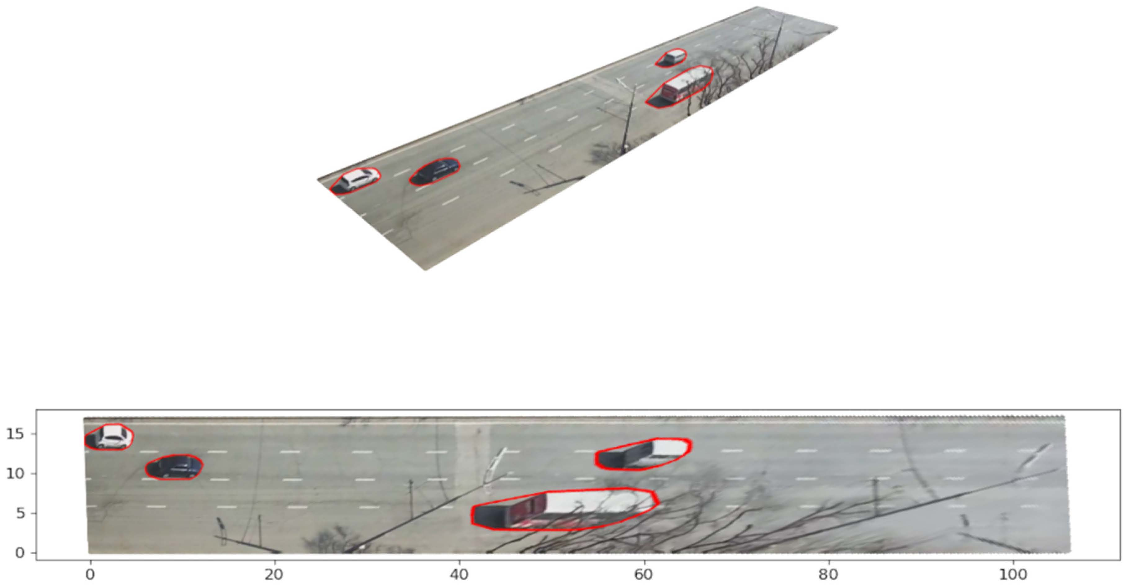
Since $Q_{\pi }\subset \mathsf{\Pi }$, the point set is suitable to output in a plane picture. If for each point, we use $\xi \left(g\right)\in Q_{\pi }$ and the color of the pixel g for all $g\in {\widehat{Q}}_{im}\subset \widehat{\mathsf{\Phi }}$, and output the plane as the scatter map, we obtain the bottom image from Figure 6. We chose a multi-car scene in the center of Q for the demonstration. We obtain the accurate ”view from above” for the points that initially lie on the road’s surface. The positions of the pixels representing objects that tower above plane $\mathsf{\Pi }$ have shifted. There are options for estimating and accounting for the height of cars and other objects so that their images look realistic in the bottom image. However, this is the subject of a separate article.

It is worth paying attention to the axes of the bottom figure (they show meters). In comparison with the original (top image of Figure 6), there are noticeable perspective distortion changes in the perception of distance. The width and length of the area are in good agreement with the measurements made by the rangefinder and estimates from online maps. The horizontal lines in the image are almost parallel which indicates the good quality of $f_u$ and $f_v$. In this way, we cross-checked the camera parameters obtained earlier. Obviously, all vehicles are in contact with the road surface.

We do not need to remove distortions (radial and perspective) from all video frames to estimate traffic statistics. The object detection or instance segmentation works with original video frames in $Q_{im}$. We use the distortions compensation for traffic measurements to obtain distances in meters for selected pixels. We calculate the needed maps once for the camera parameters and Q and use them as needed for measurements. Let us demonstrate this on a specific trajectory.

The detected trajectory of the vehicle consists of 252 contours, 180 of which are in $Q_{im}$. A total of 200 contours in the image look messy, so we draw every 20th (Figure 7). We deliberately did not choose rectangles to demonstrate a more general case. Vertex coordinates describe the contour. It is enough to select one point on or inside each contour to evaluate the speed or acceleration of an object. The point should not move around the object; we want the point source closer to the road’s surface. The left bottom corner of a contour is well suited for this camera. However, what does it mean for a polygon? For a contour ${\left\{(u_i,v_i)\right\}}_i$ we can build the pixel coordinates

$$(u_{min},v_{max})=(\underset{i}{min}{u}_i,\underset{i}{max}\left(v_i\right)).$$

We call the left bottom corner of a contour the vertex $(u_j,v_j)$ for that

$$j=\underset{i}{arg\; min}|(u_i,v_i)-(u_{min},v_{max})|,$$

considering the axes direction of the $F_{im}$. Another option is to search the point nearest to $(u_{min},v_{max})$ on the edges of the contour with the help of (19).

We map all contour vertexes on the $Q_{\pi }$ to obtain Figure 8. However, we need to map only these “corners” for measurements.

The “corners” of the selected contours have the following $y_{\pi }$ coordinates after the mapping:

$$\{-1.05,10.13,23.72,35.66,48.63,61.80,74.20,86.15,99.6\}.$$

We can use a variety of formulas to estimate speed, acceleration, and variation. The simplest estimation of the vehicle speed is (the camera frame rate is 25 frames/second, we use 1/20 of the frames):

$$=(25/20)\ast (99.6+1.05)/8=15.72656 \mathrm{m}/\mathrm{s}$$

or $56.6$ km/h.

5.2. Example 2. More Radial Distortion and Vegetation, More Calibration Points

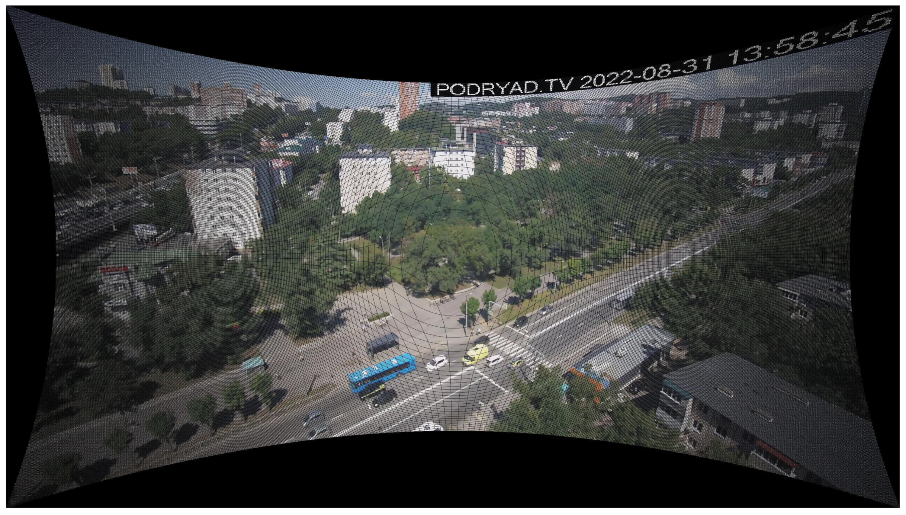
Figure 9 illustrates a frame image from another public camera of the same operator. This camera has zero horizon tilt and more substantial radial distortion. We have calibrated the camera and calculated the maps in the season of rich vegetation. Tree foliage complicates the selection and estimation of coordinates of points. The two-way road is visible to the camera. This is a FullHD camera ($N=1920,M=1080,c_u=N/2,c_v=M/2$). The zero horizon tilt is visible on the line $u=c_u$ near $P_5^v$ (see

Table 4. The points used for the calibration. Latitude and longitude are in degrees, altitudes and ENU coordinates are in meters, and coordinates of pixels are in $F_{im}$ units (u is the column index, v is the row).

Name	Lat	Long	Height	u	v	${\mathit{x}}_{\mathit{enu}}$	${\mathit{y}}_{\mathit{e}\mathit{n}\mathit{u}}$	${\mathit{z}}_{\mathit{enu}}$
$P^0$	$43.168143°$	$131.916257°$	14			0	0	0
G	$43.168356°$	$131.916733°$	25	960	540	$38.7$	$23.66$	$11$
O	$43.167616°$	$131.916245°$	56			$-0.97$	$-58.54$	$42$
$P_1^u$	$43.168775°$	$131.916107°$	18	306	540	$-12.2$	$70.2$	$4$
$P_2^v$	$43.168361°$	$131.916740°$	15	960	671	$39.27$	$24.22$	$0.7$
$P_3^u$	$43.168330°$	$131.917431°$	14	1559	540	$116.61$	$25.89$	$0$
$P_4^v$	$43.168200°$	$131.916631°$	$13.5$	960	815	$30.41$	$6.33$	$0$
$P_5^v$	$43.169134°$	$131.917249°$	43	960	199	$80.67$	$110.1$	$27$

). We select the point $P^0$ as the origin of $F_{enu}$ (see Table 4). We assess global coordinates of the point O (the camera position), point G (the source of the principal point C, Figure 1, Figure 9), and points $P_1^u,P_2^v,P_3^u,P_4^v,$ and $P_5^v$ on the lines $v=c_v$ (index u) or $u=c_u$ (index v). Next, we convert the global coordinates to $F_{enu}$ and append them to Table 4.

We obtained estimations $f_u^1=1161.93,f_v^2=1382.45,f_u^3=1168.78,f_v^4=1354.82,$ and $f_v^5=1349.67$ using Formulas (15) and (16) and Table 4 data. There are a few points, but one can assume a pattern $f_v>f_u$. Perhaps the camera’s sensor pixel has a rectangular shape (see (4)). Consider the two hypotheses:

$$f_u=(f_u^1+f_u^3)/2=1165.355,f_v=(f_v^2+f_v^4+f_v^5)/3=1362.313;$$

(50)

$$f_u=f_v=(f_u^1+f_u^3+f_v^2+f_v^4+f_v^5)/5=1283.53.$$

(51)

The second variant means the square pixel.

Let us try variant (50). With $f_u$ and $f_v$ we obtained the intrinsic parameters matrix A (1). We estimate radial distortion coefficients $k_1$ and $k_2$, put $k_1=-0.17$ and $k_2=0.01$ to compute the mapping $\mathsf{\Theta }$ (17), and apply it to eliminate radial distortion from the ($\mathsf{\Phi }$). We obtained the undistorted image $\widehat{\mathsf{\Phi }}$ (see Figure 10). We showed a cropped and interpolated version of $\mathsf{\Phi }$ in Example 1 (Figure 4). Let us demonstrate the result of mapping $\mathsf{\Theta }$ without postprocessing. The image’s resolution $\widehat{\mathsf{\Phi }}$ is $2935\times 1651$, but it contains only $1920\times 1080$ pixels colored by the camera. So, the black grid is the unfilled pixels of the large rectangular.

Let us return to the illustration that is more pleasing to the eye by cutting off part of $\widehat{\mathsf{\Phi }}$ and filling the void with interpolation (see Figure 11).

We noted that in the field of view of the camera, there is a section of the wall of the building (near $P_5^u$), allowing you to put $\gamma =0$ (see Figure 9). We are ready to compute the orientation matrix R (20)–(26), so we can convert $F_{enu}$ coordinates to $F_c$ (27). We select the points to approximate the road surface (see

Table 5. The points used to approximate road plane $\mathsf{\Pi }$ (global and $F_c$ coordinates, $F_c$ and altitudes given in meters).

Num	Lat	Long	Height	${\mathit{x}}_{\mathit{c}}$	${\mathit{y}}_{\mathit{c}}$	${\mathit{z}}_{\mathit{c}}$
1	$43.168145°$	$131.916262°$	$13.5$	$0$	$0$	$-0.1$
2	$43.168192°$	$131.916673°$	$13.5$	$33.82$	$5.44$	$-0.1$
3	$43.168275°$	$131.917036°$	14	$63.34$	$14.67$	$-0.1$
4	$43.168367°$	$131.917515°$	$14.3$	$102.29$	$24.89$	$-0$
6	$43.168519°$	$131.918425°$	15	$176.29$	$41.77$	$0.1$
7	$43.167925°$	$131.916348°$	14	$7.4$	$-24.22$	$-0.1$
8	$43.168005°$	$131.916540°$	14	$23.01$	$-15.33$	$-0.1$
9	$43.168011°$	$131.916699°$	14	$35.94$	$-14.66$	$-0.1$
10	$43.168110°$	$131.917060°$	14	$65.3$	$-3.67$	$-0.1$
11	$43.168210°$	$131.917540°$	$14.5$	$104.33$	$7.44$	$-0.1$

).

We calculate road plane $\mathsf{\Pi }$ with (29) and (32):

$$p=(0.00006008,2.93113699,130.65768737).$$

(52)

We choose four corners of $g_1,g_2,g_3,$ and $g_4$ of ${\widehat{Q}}_{im}$ in the image $\widehat{\mathsf{\Phi }}$ (see

Table 6. Domain ${\widehat{Q}}_{im}$ corners coordinates in $\widehat{\mathsf{\Phi }}$, Example 2.

Corner	Name	u	v
top left	$g_1$	509	962
bottom left	$g_2$	993	1078
top right	$g_3$	1630	498
bottom right	$g_4$	1858	558

and Figure 12). Let us try the nonrectangular area ${\widehat{Q}}_{im}$.

We calculate the lines that bound domain ${\widehat{Q}}_{im}$ with (41) and detect the set of pixel coordinates that belongs to ${\widehat{Q}}_{im}$. We compute the $Q_c$ as $\xi \left({\widehat{Q}}_{im}\right)$ with (48) and (35)–(39). Next, we convert the pixel coordinates from $Q_c$ to $F_{\pi }$ with (43)–(47) and (49) and save the result.

The distances in Q correspond to estimates obtained online and a simple rangefinder (accuracy up to a meter). We plan more accurate assessments using the geodetic tools.

We repeat the needed steps for hypothesis (51) and compare the results (see Figure 12 and Figure 13).

We observed a change in the geometry of $Q_{\pi }$ for the hypothesis (51). For example, the pedestrian crossing changed its inclination; the road began to expand to the right. In this example, it is not easy to obtain several long parallel lines due to vegetation, and it is an argument for examining the cameras in a suitable season.

6. Conclusions

This work is an extension of the technology of road traffic data collection described in [4] to allow accurate car density and speed measurements using physical units with compensation for perspective and radial distortion.

Although we processed video frames in the article, all the mappings obtained for measurements ($\mathsf{\Theta },\xi ,\left[R\right|t],R_{c2\pi }$) transform only coordinates. We used the pixel content of the images only for demonstrations. In the context of measurements, object detection (or instance segmentation) and object tracking algorithms work with pixel colors. The mappings work with the pixel coordinates of the results of these algorithms. We can calculate the discrete maps once and use them until the camera parameters or the Q area change. In this sense, the computational complexity of mapping generation is not particularly important. We plan to refine estimates of camera parameters as new data on the actual geometry of the ROI area will be available, and the accuracy of the maps will increase. Evaluating or refining the camera parameters in a suitable season might be better.

References

- Xinqiang, C.; Shubo, W.; Chaojian, S.; Yanguo, H.; Yongsheng, Y.; Ruimin, K.; Jiansen, Z. Sensing Data Supported Traffic Flow Prediction via Denoising Schemes and ANN: A Comparison. IEEE Sens. J. 2020, 20, 14317–14328. [Google Scholar]
- Xiaohan, L.; Xiaobo, Q.; Xiaolei, M. Improving Flex-route Transit Services with Modular Autonomous Vehicles. Transp. Res. Part E Logist. Transp. Rev. 2021, 149, 102331. [Google Scholar]
- 75 Years of the Fundamental Diagram for Traffic Flow Theory: Greenshields Symposium TRB Transportation Research Electronic Circular E-C149. 2011. Available online: http://onlinepubs.trb.org/onlinepubs/circulars/ec149.pdf (accessed on 17 September 2022).
- Zatserkovnyy, A.; Nurminski, E. Neural network analysis of transportation flows of urban agglomeration using the data from public video cameras. Math. Model. Numer. Simul. 2021, 13, 305–318. [Google Scholar]
- Camera Calibration and 3D Reconstruction. OpenCV Documentation Main Modules. Available online: https://docs.opencv.org/4.5.5/d9/d0c/group__calib3d.html (accessed on 18 March 2022).
- Szeliski, R. Computer Vision: Algorithms and Applications, 2nd ed.; Springer: Cham, Switzerland, 2022. [Google Scholar]
- Hartley, R.; Zisserman, A. Multiple View Geometry in Computer Vision, 2nd ed.; Cambridge University Press: New York, NY, USA, 2003. [Google Scholar]
- Transformations between ECEF and ENU Coordinates. ESA Naupedia. Available online: https://gssc.esa.int/navipedia/index.php/Transformations_between_ECEF_and_ENU_coordinates (accessed on 18 March 2022).
- Forsyth, D.A.; Ponce, J. Computer Vision: A Modern Approach, 2nd ed.; Pearson: Hoboken, NJ, USA, 2012. [Google Scholar]
- Peng, S.; Sturm, P. Calibration Wizard: A Guidance System for Camera Calibration Based on Modeling Geometric and Corner Uncertainty. arXiv 2019, arXiv:1811.03264. [Google Scholar]
- Camera Calibration. OpenCV tutorials, Python. Available online: http://docs.opencv.org/4.x/dc/dbb/tutorial_py_calibration.html (accessed on 18 March 2022).
- Marchand, E.; Uchiyama, H.; Spindler, F. Pose estimation for augmented reality: A hands-on survey. IEEE Trans. Vis. Comput. Graph. 2016, 22, 2633–2651. [Google Scholar] [CrossRef] [PubMed] [Green Version]
- Perspective-n-Point (PnP) Pose Computation. OpenCV documentation. Available online: https://docs.opencv.org/4.x/d5/d1f/calib3d_solvePnP.html (accessed on 18 March 2022).
- Liu, C.-M.; Juang, J.-C. Estimation of Lane-Level Traffic Flow Using a Deep Learning Technique. Appl. Sci. 2021, 11, 5619. [Google Scholar] [CrossRef]
- Khazukov, K.; Shepelev, V.; Karpeta, T.; Shabiev, S.; Slobodin, I.; Charbadze, I.; Alferova, I. Real-time monitoring of traffic parameters. J. Big Data 2020, 7, 84. [Google Scholar] [CrossRef]
- Zhengxia, Z.; Zhenwei, S. Object Detection in 20 Years: A Survey. arXiv 2019, arXiv:1905.05055v2. [Google Scholar]
- Huchuan, L.; Dong, W. Online Visual Tracking; Springer: Singapore, 2019. [Google Scholar]
- Yandex Maps. Available online: https://maps.yandex.ru (accessed on 18 March 2022).
Figure 1.
Coordinate frames , . are the image of the 3D point P. Axis follows the camera optical axis. The camera forms a real image on the image sensor behind aperture O in the plane ; however, the equivalent virtual image in the plane is preferable in illustrations.
Figure 2.
Virtual and real images for a camera with aperture O. The scene is projected on the plane of frame . The coordinates of the point P in are denoted by , and the are coordinates of points on the axis U of frame .
Figure 3.
Field of view of the public street camera in Vladivostok. Example 1, image .
Figure 4.
The image after compensation of radial distortion. Example 1, image .
Figure 5.
The image rotated by around the optical axis of the camera.
Figure 6.
The set visualization in plane , by the colors of the pixels from . Given the geometry of the sample, is the horizontal axis, the vertical.
Figure 7.
Every twentieth contour of a vehicle’s trajectory in the original image .
Figure 8.
Every twentieth contour in the vehicle’s trajectory mapped on the with the selected points.
Figure 9.
Field of view of the public street camera in Vladivostok. Example 2, image .
Figure 10.
The image after compensation of radial distortion; Example 2, image without postprocessing.
Figure 11.
Cropped and interpolated part of image .
Figure 12.
The set visualization in plane for case (50).
Figure 13.
The set visualization in plane for case (51).