Mathematical Modelling of Diffusion Flows in Two-Phase Stratified Bodies with Randomly Disposed Layers of Stochastically Set Thickness

Abstract

The work is dedicated to mathematical modelling of random diffusion flows of admixture particles in a two-phase stratified strip with stochastic disposition of phases and random thickness of inclusion-layers. The study of such models are especially important during the creation of composite layered materials, in the research of the transmission properties of filters, and in the prediction of the spread of pollutants in the environment. Within the model we consider one case of uniform distribution of coordinates of upper boundaries of the layers of which the body is made up and two more cases, i.e., of uniform and triangular distributions of the inclusion thickness. The initial-boundary value problems of diffusion are formulated for flux functions; the boundary conditions at one of the body’s surfaces are set for flux and, at the other boundary, the conditions are given for admixture concentration; the initial condition being concerned with zero and non-zero constant initial concentrations. An equivalent integro-differential equation is constructed. Its solution is found in terms of Neumann series. For the first time it was obtained calculation formulae for diffusion flux averaged over the ensemble of phase configurations and over the inclusion thickness. It allowed to investigate the dependence of averaged diffusion fluxes on the medium’s characteristics on the basis of the developed software. The simulation of averaged fluxes of admixture in multilayered $Fe-Cu$ and $\alpha Fe-Ni$ materials is made. Comparative analysis of solutions, depending on the stage of averaging procedure over thickness, is carried out. It is shown that for some values of parameters the stage of averaging procedure over thickness has almost no effect on the diffusion flow value.

1. Introduction

Estimation of longevity and effectiveness of regimes of operation of water filters, study of permeable capacity of membranes [1,2], investigation of functional characteristics of composite materials [3,4,5] and reliability of engineering structures [6,7], etc., are based on modelling the processes of mass transfer which occur in them. In modelling such objects as multiphase stratified bodies, the coordinates of location of inclusions, as well as their sizes, can be unknown. Therefore, there is a need to consider these structures as randomly non-homogeneous ones [8].

In mathematical descriptions of such random processes, the application of averaging procedure over the ensemble of phase configurations in order to find the mass transfer characteristic, such as diffusion flux, is very difficult. Since the function of correlation of random diffusion coefficient and gradient of stochastic field of concentration is unknown.

To solve this problem, some authors [9,10] suggest first to construct balance equations for porous bodies for homogenized media whose physical characteristics are averaged magnitudes. In this case they take into account the difference between coefficients of the phases and, at the same time, herewith interaction of phases is neglected. Notice that methods of homogenization or statistical averaging are applicable when the number of non-homogeneities of the structure is macroscopic, their probability distribution is close to uniform, the change of the investigated fields at distances exceeding the dimensions of the non-homogeneities is insignificant [11,12,13,14,15]. In the works [16,17,18], the processes of heat transfer and diffusion in one-dimensional periodical stratified structures are studied on the basis of the method of homogenization. Additionally, in papers [19,20] on modelling transport processes in heterogeneous structures, it was proposed to use a discrete model with subsequent reduction using homogenization methods, in particular, to a linear stationary problem. In the investigation [21], the random flow is determined according to the Darcy law with a filtration coefficient being a function of a spatial coordinate. For constructing the problem solution, the methods of both small perturbations and smoothing (with the corresponding restrictions) are applied. Additionally, they also impose the condition of the normal distribution of phases, which makes it impossible to determine the averaged mass flux. Proceeding in such a way, the author defines the two-point function of covariation only.

To solve this problem, we proposed an original approach to the description of diffusion flows in randomly non-homogeneous layered structures according to which we formulate initial-boundary value problems immediately in terms of the flux [22]. Within this approach, a new diffusion equation for the flow function in which non-homogeneity of the structure takes into account in its coefficients is constructed [23]. However, within the scope of such an approach it is necessary to formulate reasonable initial and boundary conditions. Because, in the case where values of the flux on the “top” boundary of the body are much greater than those on the “bottom” one, an unlimited amount of diffusing substance can enter a limited body. Additionally, that is a certain contradiction. Similarly, while maintaining a much greater flux through the “bottom” boundary of the layer we also come to a certain contradiction. In this regard, we suggest to set the value of mass flux at one body’s surface; at the other surface we set the value of substance concentration and, further, we determine the corresponding condition for the flux.

The purpose of this work is to investigate for the first time random flows of admixture substance in two-phase stochastically non-homogeneous stratified bodies under uniform distribution of phases and also for two cases of (uniform and triangular) distributions of random thickness of inclusions. For this aim, the next steps should be completed:

• Build a mathematical model of admixture diffusion in a two-phase body with randomly located inclusions of stochastic thickness based on the diffusion equation for the flow function, the coefficients of which take into account the non-homogeneity of the structure. Consider both two cases of zero and non-zero constant initial concentration of admixture;
• Obtain an integro-differential equation equivalent to the initial-boundary value diffusion problem;
• Construct the solution to this equation in the form of absolutely and uniformly convergent Neumann series;
• Carry out the procedure of averaging over the ensemble of phase configurations with a uniform distribution function of inclusions in the body;
• Average the obtained result over the random thickness of the layers for uniform and triangular distributions of the inclusion’s thickness;
• Development of software modules and carrying out a numerical study to establish the main regularities of the behaviour of the diffusion flow;
• Application of the obtained model for calculation of hydrogen flows in layered bimetallic composites.

2. Research Methods

To construct the diffusion equation for the flow function, the balance equations of thermodynamics of nonequilibrium processes are used. Formulation and justification of the boundary conditions of the problem, which correspond to real mass transfer processes occurring in the environment, is carried out using the results and methods of analytical chemistry and mathematical physics. The equivalent integro-differential equation is constructed by the methods of mathematical physics, taking into account the conditions and restrictions of probability theory. To find expressions for the flow in a homogeneous body (without inclusions) at zero and non-zero constant initial concentration, as well as Green function, we use the methods of integral transformations, namely, we carry out the Fouret transformation with respect to the spatial variable and the Laplace transformation with respect to time. The solution to the equivalent integro-differential equation is obtained in the form of Neumann series by a successive iterations method. The methods of probability theory, mathematical statistics, and mathematical analysis are used for the averaging procedure over the ensemble of phase configurations and over the random thickness of the layer. Software development for the numerical implementation of research includes the creation of the following modules

• Two modules to calculate the diffusion flow in the homogeneous strip without inclusions under zero and non-zero initial concentration;
• The module for Green function calculation;
• Two modules for calculation of the diffusion flow in multilayered strip with uniform distribution of layer’s thickness for zero and non-zero initial concentration of migrating particles;
• Two modules to calculate the diffusion flow in the non-homogeneous strip with triangular distribution of layer’s thickness for zero and non-zero initial concentration of migrating particles.

In the development of these modules, the free software compiler for Fortran code Gfortran was used. All codes were run under work station Ms AMD Ryzen 5 3.6 GHz/ Gigabyte GA-AB350M/DDR4 8 Gb/HDD 1000 Gb/GeForse GT730 1 GB/ATX 450 W/K + M (Manufactured by GIGA-BYTE Technology Co., Ltd, Nan-Ping, Taiwan).

3. Mathematical Model

3.1. Formulation of the Mathematical Model

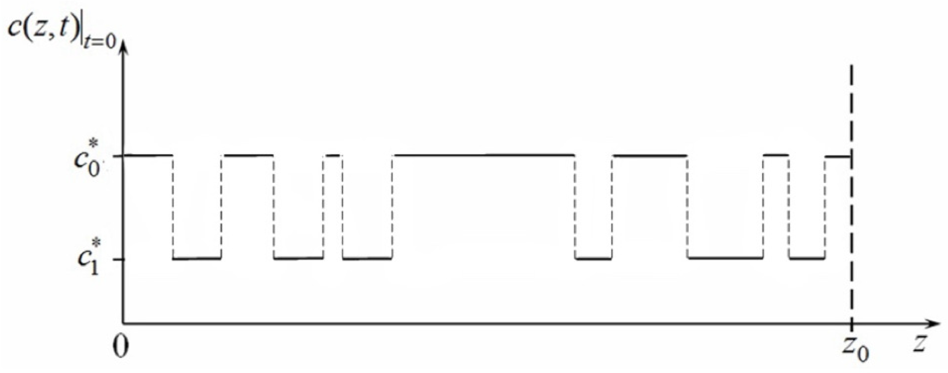
Let admixture particles be migrating in a strip of the thickness $z_0$ containing $n_0$ layers of matrix and $n_1$ layers of inclusions of stochastic thickness (Figure 1a). The layers’ coordinates are unknown. In each phase, diffusion coefficients are constant and the same. Let the fraction of the basic phase $v_0$ in terms of volume is much greater than the fraction of inclusions $v_1$ in terms of volume: $v_0>>v_1.$ We assume that phases dispose in the body under uniform distribution and the inclusion thickness $h_{i1}$ is a random quantity with the given function of distribution on the interval $[h_{min};h_{max}]$, $0<h_{min}<h_{max}<z_0$ (Figure 1b).

From the equation for concentration balance ${\displaystyle \frac{\partial c(\overrightarrow{r},t)}{\partial t}=-\overrightarrow{\nabla }·\overrightarrow{J}(\overrightarrow{r},t)}$ [24] and kinetic relation between mass flow and gradient of concentration (of the Fick law type) [25]

$$\overrightarrow{J}(\overrightarrow{r},t)=-D\left(\overrightarrow{r}\right)\overrightarrow{\nabla }c(\overrightarrow{r},t)$$

(1)

We obtain the partial differential equation for the mass flow function. Then, assuming that the diffusion coefficient $D\left(\overrightarrow{r}\right)$ is time-independent, we have

$$\frac{\partial \overrightarrow{J}(\overrightarrow{r},t)}{\partial t}=D\left(\overrightarrow{r}\right)\overrightarrow{\nabla }\otimes \overrightarrow{\nabla }·\overrightarrow{J}(\overrightarrow{r},t),$$

(2)

where $\overrightarrow{J}(\overrightarrow{r},t)$ is the mass flux of the diffusing substance; $D\left(\overrightarrow{r}\right)$ is the diffusion coefficient; $c(\overrightarrow{r},t)$ is the admixture concentration; $\overrightarrow{\nabla }$ is Hamilton nabla-operator; ⊗ is the sing of the tensor multiplication; $\overrightarrow{r}$ is the radius-vector of the running point, t is the time; and operation of scalar multiplication is marked with a dot.

We formulate the initial-boundary value problem which corresponds to one-dimensional case. To avoid possible contradictions [22], we suggest to set the value of mass flux at one surface of the body and the values of admixture concentration at the other surface.

In one-dimensional (with respect to spatial coordinate) case, the Equation of admixture diffusion (2) formulated for mass flow function in a multiphase body is reduced to the following equation [25]:

$$\frac{\partial J(z,t)}{\partial t}=D\left(z\right)\frac{{\partial }^{2}J(z,t)}{\partial z^2}.$$

(3)

Here $D\left(z\right)=\left\{\begin{array}{cc}{D}_0,\hfill & z\in {\Omega }_0\hfill \\ D_1,\hfill & z\notin {\Omega }_0\hfill \end{array}\right.$ is the stochastic coefficient of admixture diffusion, ${\Omega }_j$ is the multi-connected domain of the j-th phase, j = 0; 1 (Figure 1a); $\sum _j{\Omega }_j=\Omega$, where $\Omega$ is the domain of the whole body.

3.2. Initial and Boundary Conditions of the Problem

Let at the initial instant of time the diffusion flow be absent in the body. The constant diffusion flow is kept at the body’s boundary z = 0, and the admixture concentration equals zero at the lower surface $z=z_0$ of the strip. Namely, the following initial and boundary conditions are given:

$$J(z,t){|}_{t=0}=0;$$

(4)

$$J(z,t){|}_{z=0}=J_{*}\equiv const,c(z,t){|}_{z=z_0}=0.$$

(5)

Herewith, the diffusion flux at the lower boundary is a certain function of time $F\left(t\right)$ which is to be determined additionally

$$J(z,t){|}_{z=z_0}=F\left(t\right).$$

(6)

The initial condition for the concentration of admixture particles equivalent to the initial condition for flow of the Substance (4) can be obtained from the first Fick law for the chemical potential $\mu (z,t)$ (namely, ${\displaystyle J(z,t)=-\tilde{L}\left(z\right)\frac{\partial \mu (z,t)}{\partial z}}$[26], where $\tilde{L}\left(z\right)$ is kinetic coefficient of mass transfer), from relation between chemical potential and concentration (in the linearized form of the relation $\mu (z,t)={\mu }^0+Aln\gamma \left(z\right)c(z,t)$ [26]), and from the initial condition for chemical potential of admixture [26,27]. Then, we obtain the following condition:

$$c(z,t){|}_{t=0}=\left\{\begin{array}{cc}[1+({\mu }_{*}-{\mu }^0)/A]/{\gamma }_0,\hfill & z\in {\Omega }_0\hfill \\ [1+({\mu }_{*}-{\mu }^0)/A]/{\gamma }_1,\hfill & z\notin {\Omega }_0\hfill \end{array}\right..$$

(7)

Here, ${\mu }_{*}$ is the value of chemical potential at the initial instant of time, i.e., $\mu (z,t){|}_{t=0}={\mu }_{*}\equiv const$; ${\mu }^0$ is the chemical potential of pure substance in the state which is determined by values of the absolute temperature T and the pressure P; $A=RT/M$ is the coefficient, here R is the absolute gas constant, M is the atomic weight of the element of admixture; $\gamma \left(z\right)$ is the coefficient of activity, which can be presented for a two-phase body as $\gamma \left(z\right)=\left\{\begin{array}{c}{\gamma }_0,z\in {\Omega }_0\hfill \\ {\gamma }_1,z\in {\Omega }_1\hfill \end{array}\right.$.

Denote $c_j^{*}=[1+({\mu }_{*}-{\mu }^0)/A]/{\gamma }_j$$(j=0;1)$. Then, $c(z,t){|}_{t=0}=\{c_j^{*}\equiv const,z\in {\Omega }_j\}$. We have obtained a piecewise-constant function for the initial concentration, schematic drawing of which is shown in Figure 2. In this graph, the y-axis represents function $c(z,t){|}_{t=0}$, the x-axis represents the spatial coordinate z. Notice that there are jumps discontinuities of admixture concentration function at the initial time on the boundaries of contact of the domains ${\Omega }_j$ (Figure 2).

Notice that the quantity $c(z,t){|}_{t=0}$ can be both random and deterministic, depending on stochasticity or determinacy of the domain $\Omega$. Henceforth, assume that the disposition of the domains ${\Omega }_j$ is unknown, i.e., coordinates of layer locations are random.

If in different phases the coefficients of activity are close, i.e., if we can assume that ${\gamma }_0\approx {\gamma }_1\equiv {\gamma }_{*}$, then $c_0^{*}\approx c_1^{*}\equiv c_{*}$, and the Condition (7) is the following

$$c(z,t){|}_{t=0}=c_{*}\equiv const.$$

(8)

Henceforth, we shall consider the initial condition for the admixture concentration function in the Form (8), and singling out the separate case of absence of admixture substance at the initial instant of time in a body

$$c(z,t){|}_{t=0}=0.$$

(9)

Further, we shall consider only the initial Conditions (8) and (9).

Note that according to this approach, a random structure of the medium is taken into account by means of the diffusion coefficient of migrating substance, which is a stochastic function of the spatial coordinates.

4. Construction of the Problem Solution

To construct the solution of the initial-boundary value Problem (3)–(6) with the random diffusion coefficient, we present this coefficient in terms of the following random “function of structure” [28] ${\eta }_{ij}\left(z\right)=\left\{\begin{array}{cc}1,\hfill & z\in {\Omega }_{ij}\hfill \\ 0,\hfill & z\notin {\Omega }_{ij}\hfill \end{array}\right.$, where ${\Omega }_{ij}$ is the i-th simply connected domain of the kind j, and ${\displaystyle \bigcup _{i=1}^{n_j}{\Omega }_{ij}={\Omega }_j}$$(j=0;1,i=1,\cdots ,n_j)$. Then, the coefficient of admixture diffusion $D\left(z\right)$ takes the following: $D\left(z\right)={\displaystyle \sum _{i=1}^{n_0}}{D}_0{\eta }_{i0}\left(z\right)+{\displaystyle \sum _{i=1}^{n_1}}{D}_1{\eta }_{i1}\left(z\right)$.

Herewith ${\displaystyle \sum _{i=1}^{n_0}}{\eta }_{i0}\left(z\right)+{\displaystyle \sum _{i=1}^{n_1}}{\eta }_{i1}\left(z\right)=1$ (the condition of body continuity). Notice that the choice of the number i of simply connected domains both of matrix and of inclusion is conventional.

Substituting such a representation of the coefficient $D\left(z\right)$ into Equation (3) we obtain:

$$\frac{\partial J(z,t)}{\partial t}-\left({\displaystyle \sum _{i=1}^{n_0}}{D}_0{\eta }_{i0}\left(z\right)+{\displaystyle \sum _{i=1}^{n_1}}{D}_1{\eta }_{i1}\left(z\right)\right)\frac{{\partial }^{2}J(z,t)}{\partial z^2}=0.$$

(10)

In Equation (10) we add and subtract the deterministic operator $L_0(z,t)$ defined as:

$$L_0(z,t)\equiv \frac{\partial }{\partial t}-D_0\frac{{\partial }^2}{\partial z^2}.$$

Then, denoting the operator of Equation (10) in the following form

$$L(z,t)\equiv \frac{\partial }{\partial t}-\left({\displaystyle \sum _{i=1}^{n_0}}{D}_0{\eta }_{i0}\left(z\right)+{\displaystyle \sum _{i=1}^{n_1}}{D}_1{\eta }_{i1}\left(z\right)\right)\frac{{\partial }^2}{\partial z^2},$$

Additionally, taking into account for the condition of continuity of the body, we obtain:

$$L_0(z,t)J(z,t)=L_s(z,t)J(z,t),$$

(11)

where $L_s(z,t)\equiv L_s\left(z\right)=(D_1-D_0){\displaystyle \sum _{i=1}^{n_1}}{\eta }_{i1}\left(z\right){\partial }^2/\partial z^2$.

We should find the solution of the initial-boundary value Problem (4), (5), and (11) in the form of Neumann series.

Considering non-homogeneities of the structure of a body as inner sources the solution of the initial-boundary value Problem (4), (5), and (11) can be presented as the sum of the solution of homogeneous problem and convolution of Green function with the source

$$J(z,t)=J_0(z,t)+\underset{0}{\overset{t}{\int }}\underset{0}{\overset{z_0}{\int }}G(z,z^{\prime },t,t^{\prime })L_s\left(z^{\prime }\right)J(z^{\prime },t^{\prime })d{z}^{\prime }d{t}^{\prime },$$

(12)

where $J_0(z,t)$ is the solution of the homogeneous initial-boundary value Problem, $G(z,z^{\prime },t,t^{\prime })$ is Green function of the problem (4), (5), and (11), which is a deterministic function.

To find the solution of the homogeneous initial-boundary value problem

$$\frac{\partial J_0(z,t)}{\partial t}=D_0\frac{{\partial }^2{J}_0(z,t)}{\partial z^2};$$

$$J_0(z,t){|}_{t=0}=0;J_0(z,t){|}_{z=0}=J_{*}\equiv const,J_0(z,t){|}_{z=z_0}=F\left(t\right),$$

We must first determine the boundary condition for the flow function at the boundary $z=z_0$. For this purpose, we solve the initial-boundary value problem formulated for the function $c(z,t)$ of migrating particle concentration. If at the initial instant of time the distribution of the concentration equals zero, the initial-boundary problem is as following

$$\frac{\partial c(z,t)}{\partial t}=D_0\frac{{\partial }^{2}c(z,t)}{\partial z^2};$$

(13)

$$\partial c(z,t)/\partial z{|}_{z=0}=-J_{*}/D_0\equiv const,c(z,t){|}_{z=z_0}=0;$$

(14)

$$c(z,t){|}_{t=0}=0.$$

(15)

If at the initial instant of time the constant non-zero distribution of concentration in the strip is set, then the Condition (15) takes the form

$$c(z,t){|}_{t=0}=c_{*}\equiv const.$$

(16)

The solution of the problem with zero initial concentration is obtained in the form [29]:

$$c(z,t)=\frac{J_{*}}{D_0}\left(z_0-z-\frac{2}{z_0}{\displaystyle \sum _{n=1}^{\infty }}\frac{e^{-D_0{\xi }_n^{2}t}cos\left({\xi }_{n}z\right)}{{\xi }_n^2}\right).$$

(17)

and for non-zero constant initial concentration the solution is found as follows:

$$c(z,t)=\frac{J_{*}}{D_0}(z_0-z)-\frac{2}{z_0}\sum _{n=1}^{\infty }{e}^{-D_0{\xi }_n^{2}t}\left(\frac{J_{*}}{D_0{\xi }_n^2}+\frac{c_{*}{(-1)}^n}{{\xi }_n}\right)cos\left({\xi }_{n}z\right),$$

(18)

where ${\xi }_n=\pi (2n-1)/2z_0$.

Taking into account the first Fick law (1), from the Solution (17) of the initial-boundary value Problem (13)–(15) we obtain the following expression for the homogeneous strip:

$$J_0(z,t)=J_{*}\left(1-\frac{2}{z_0}\sum _{n=1}^{\infty }\frac{1}{{\xi }_n}{e}^{-D_0{\xi }_n^{2}t}sin\left({\xi }_{n}z\right)\right).$$

(19)

In particular, at the boundary $z=z_0$ we have:

$$J_0(z,t){|}_{z=z_0}\equiv F\left(t\right)=J_{*}\left(1-\frac{2}{z_0}\sum _{n=1}^{\infty }\frac{1}{{\xi }_n}{(-1)}^{n+1}{e}^{-D_0{\xi }_n^{2}t}\right).$$

(20)

Similarly, for the initial-boundary value Problem (13), (14), and (16) from the Expression (18) we find

$$J_0(z,t)=J_{*}-\frac{2}{z_0}\sum _{n=1}^{\infty }{e}^{-D_0{\xi }_n^{2}t}\left(\frac{J_{*}}{{\xi }_n}+D_0{c}_{*}{(-1)}^n\right)sin\left({\xi }_{n}z\right),$$

(21)

and for $z=z_0$ we obtain the following boundary condition for the diffusion function flux:

$$J_0(z,t){|}_{z=z_0}\equiv \tilde{F}\left(t\right)=J_{*}-\frac{2}{z_0}\sum _{n=1}^{\infty }{(-1)}^{n+1}{e}^{-D_0{\xi }_n^{2}t}\left(\frac{J_{*}}{{\xi }_n}+D_0{c}_{*}{(-1)}^n\right).$$

(22)

Analyzing the Formulae (20) and (22), we can affirm that, in the case of zero initial concentration, $F\left(t\right)$ is a steadily increasing function. However, at certain constant non-zero initial concentration the function $\tilde{F}\left(t\right)$ sharply decreases and after reaching a local minimum begins to increases. In addition, the higher the value of $c_{*}/J_{*}$, the sooner the function $F\left(t\right)$ gets on the steady-state regime.

Green function has the form [23]:

$$G(z,z^{\prime },t,t^{\prime })=\frac{\theta (t-t^{\prime })}{z_0}\sum _{k=1}^{\infty }{e}^{-D_0{y}_k^2(t-t^{\prime })}\left[cos\left(y_k(z-z^{\prime })\right)-cos\left(y_k(z+z^{\prime })\right)\right],$$

(23)

where $\theta (t-t^{\prime })$ is the unit step Heaviside’s function, $y_k=k\pi /z_0$.

We obtain the solution of the integro-differential Equation (12) in the form of Neumann series by means of the method of successive iterations with choosing $J_0(z,t)$ as zero iteration [30]. Because such a representation of the solution is convenient for performing the procedure of averaging over ensemble of phase configuration. Thus, we have:

$$\begin{array}{cc}\hfill J(z,t)=& J_0(z,t)+\underset{0}{\overset{t}{\int }}\underset{0}{\overset{z_0}{\int }}G(z,z^{\prime },t,t^{\prime })L_s\left(z^{\prime }\right)J_0(z^{\prime },t^{\prime })d{z}^{\prime }d{t}^{\prime }+\underset{0}{\overset{t}{\int }}\underset{0}{\overset{z_0}{\int }}G(z,z^{\prime },t,t^{\prime })\times \hfill \\ \hfill & \times L_s\left(z^{\prime }\right)\underset{0}{\overset{t^{\prime }}{\int }}\underset{0}{\overset{z_0}{\int }}G(z^{\prime },z^{″},t^{\prime },t^{″})L_s\left(z^{″}\right)J_0(z^{″},t^{″})d{z}^{″}d{t}^{″}d{z}^{\prime }d{t}^{\prime }+\cdots +\hfill \\ \hfill & +\underset{0}{\overset{t}{\int }}\underset{0}{\overset{z_0}{\int }}G(z,z^{\prime },t,t^{\prime })L_s\left(z^{\prime }\right)[\underset{0}{\overset{t^{\prime }}{\int }}\underset{0}{\overset{z_0}{\int }}G(z^{\prime },z^{″},t^{\prime },t^{″})L_s\left(z^{″}\right)\times \hfill \\ \hfill & \times \underset{0}{\overset{t^{″}}{\int }}\underset{0}{\overset{z_0}{\int }}G(z^{″},z^{‴},t^{″},t^{‴})L_s\left(z^{‴}\right)J_0(z^{‴},t^{‴})d{z}^{‴}d{t}^{‴}d{z}^{″}d{t}^{″}]d{z}^{\prime }d{t}^{\prime }+\cdots \hfill \end{array}$$

(24)

The Series (24) is absolutely and uniformly convergent if the diffusion coefficients are restricted [31], i.e., $D_0,D_1\le K<\infty$, and $D_0\ne 0$ (i.e., the diffusion process runs in the prevailing phase). The first term of the Neumann series determines the diffusion flow in the homogeneous strip of matrix characteristics. The second term is the sum of flow disturbances arising when we put into the body inclusions of the characteristics different from the matrix parameters. The term summand describes effects of pair mutual influence of inclusions on the mass flow that arise when we alternately pairwise put inclusions of another (than those of the matrix) physical parameters into the homogeneous body of the matrix characteristics, and so on.

To perform the procedures of averaging, we restrict our investigation to the two first terms of the Series (24).

5. Averaging the Solution over Ensemble of Phase Configurations

For the body structure described above, the reference initial-boundary value Problem of diffusion (3)–(5) involves two random magnitudes, namely the coordinate of inclusion location and the layer thickness. Let the coordinate characterizing the inclusion location be the coordinate of the upper boundary of the inclusion $z_{i1}(i=1,\cdots ,n_1)$. We shall firstly average the mass flow over the ensemble of phase configurations, and then perform the averaging of the obtained expression over the random thickness $h_{i1}$ of the layer ${\Omega }_{i1}$. For this purpose, we find the averaged diffusion flow in the two-phase randomly non-homogeneous strip according to the formula:

$${〈{〈J(z,t)〉}_{conf}〉}_h=J_0(z,t)+{〈\underset{0}{\overset{t}{\int }}\underset{0}{\overset{z_0}{\int }}G(z,z^{\prime },t,t^{\prime }){〈L_s\left(z^{\prime }\right)〉}_{conf}J(z^{\prime },t^{\prime })d{z}^{\prime }d{t}^{\prime }〉}_h.$$

(25)

In this formula, we have used the fact that $J_0(z,t)$ and $G(z,z^{\prime },t,t^{\prime })$ are deterministic functions. Notice that only function ${\eta }_1\left(z^{\prime }\right)$ in the operator $L_s\left(z^{\prime }\right)$ depends on the random coordinate of upper boundary of inclusion. Thus, we have:

$${〈L_s\left(z^{\prime }\right)〉}_{conf}=(D_1-D_0)\sum _{i=1}^{n_1}{〈{\eta }_{i1}\left(z^{\prime }\right)〉}_{conf}\frac{\partial }{\partial z^{\prime 2}}.$$

For uniform distribution of phases we write:

$$\sum _{i=1}^{n_1}{〈{\eta }_{i1}\left(z^{\prime }\right)〉}_{conf}=\frac{1}{V}\sum _{i=1}^{n_1}\underset{\left(V\right)}{\int }{\eta }_{i1}\left(z^{\prime }\right)d{z}_{i1}.$$

Taking into consideration the properties of the function ${\eta }_{i1}\left(z^{\prime }\right)$:

$${\eta }_{i1}\left(z^{\prime }\right)=\left\{\begin{array}{c}1,z^{\prime }\in [z_{i1};z_{i1}+h_{i1}]\hfill \\ 0,z^{\prime }\notin [z_{i1};z_{i1}+h_{i1}]\hfill \end{array}\right.=\left\{\begin{array}{c}1,z^{\prime }-z_{i1}\in [0;h_{i1}]\hfill \\ 0,z^{\prime }-z_{i1}\notin \left[0\right];h_{i1}]\hfill \end{array}\right.={\eta }_{i1}(z^{\prime }-z_{i1})$$

and performing the substitution $z^{\prime }-z_{i1}=x$, we can write:

$$\sum _{i=1}^{n_1}{〈{\eta }_{i1}\left(z^{\prime }\right)〉}_{conf}=\frac{1}{V}\sum _{i=1}^{n_1}\underset{0}{\overset{z_0-h_{i1}}{\int }}{\eta }_{i1}(z^{\prime }-z_{i1})d{z}_{i1}=\frac{1}{V}\sum _{i=1}^{n_1}\underset{0}{\overset{z^{\prime }}{\int }}{\eta }_{i1}\left(x\right)dx,$$

(26)

because ${\eta }_{i1}\left(x\right)=\left\{\begin{array}{c}1,x\in [0;h_{i1}]\hfill \\ 0,x\notin [0;h_{i1}]\hfill \end{array}\right.$. The integral in the obtained Formula (26) depends on the value of variable $z^{\prime }$ of exterior integration in the Expression (25). Therefore,

(1)

If $z^{\prime }\le h_{i1}$ then

$$\frac{1}{V}\sum _{i=1}^{n_1}\underset{0}{\overset{z^{\prime }}{\int }}{\eta }_{i1}\left(x\right)dx=\frac{1}{V}\sum _{i=1}^{n_1}\underset{0}{\overset{z^{\prime }}{\int }}dx=\frac{z^{\prime }}{z_0};$$

(2)

If $z^{\prime }\ge h_{i1}$ then

$$\frac{1}{V}\sum _{i=1}^{n_1}\underset{0}{\overset{z^{\prime }}{\int }}{\eta }_{i1}\left(x\right)dx=\frac{1}{V}\sum _{i=1}^{n_1}\underset{0}{\overset{h_{i1}}{\int }}dx=\frac{h_{i1}}{z_0}.$$

Thus, we have:

$$\sum _{i=1}^{n_1}{〈{\eta }_{i1}\left(z^{\prime }\right)〉}_{conf}=\left\{\begin{array}{c}{z}^{\prime }/z_0,z^{\prime }\le h_{i1}\hfill \\ h_{i1}/z_0,z^{\prime }\ge h_{i1}\hfill \end{array}\right..$$

(27)

Substituting (27) into the relation (25) we obtain:

$${〈{〈J(z,t)〉}_{conf}〉}_h=J_0(z,t)+\frac{(D_1-D_0)}{z_0}〈\sum _{i=1}^{n_1}\underset{0}{\overset{t}{\int }}\left[\underset{0}{\overset{h_{i1}}{\int }}{z}^{\prime }G(z,z^{\prime },t,t^{\prime })\right.\times$$

$${\left.\times \frac{{\partial }^2{J}_0(z^{\prime },t^{\prime })}{\partial z^{\prime 2}}d{z}^{\prime }+h_{i1}\underset{h_{i1}}{\overset{z_0}{\int }}G(z,z^{\prime },t,t^{\prime })\frac{{\partial }^2{J}_0(z^{\prime },t^{\prime })}{\partial z^{\prime 2}}d{z}^{\prime }\right]d{t}^{\prime }〉}_h.$$

(28)

Thus, we have averaged the diffusion flow over the ensemble of phase configurations with uniform distribution of inclusions, but we still need to average the Expression (28) over the random thickness of inclusions.

6. Averaging the Solution over Inclusion Thickness

6.1. Uniform Distribution of Inclusion Thickness

Assume that the thickness $h_{i1}$ is the random quantity with uniform distribution over the interval $[h_{min};h_{max}]$. The density of distribution of $h_{i1}$ is of $f\left(h_{i1}\right)=1/\Delta h$, where $\Delta h=h_{max}-h_{min}$. We substitute the density of the distribution into the Expression (28), integrate over the thickness, and as a result we obtain the following formula:

$${〈{〈J(z,t)〉}_{conf}〉}_{h_{i1}}=J_0(z,t)+\frac{(D_1-D_0)}{z_0}\sum _{i=1}^{n_1}\underset{h_{min}}{\overset{h_{max}}{\int }}\frac{1}{\Delta h}\underset{0}{\overset{t}{\int }}\left[\underset{0}{\overset{h_{i1}}{\int }}{z}^{\prime }G(z,z^{\prime },t,t^{\prime })\right.\times$$

$$\left.\times \frac{{\partial }^2{J}_0(z^{\prime },t^{\prime })}{\partial z^{\prime 2}}d{z}^{\prime }+h_{i1}\underset{h_{i1}}{\overset{z_0}{\int }}G(z,z^{\prime },t,t^{\prime })\frac{{\partial }^2{J}_0(z^{\prime },t^{\prime })}{\partial z^{\prime 2}}d{z}^{\prime }\right]d{t}^{\prime }d{h}_{i1}.$$

(29)

If we substitute the expressions both for Green function $G(z,z^{\prime },t,t^{\prime })$ (23) and for diffusion flow in the homogeneous body $J_0(z,t)$ (19) at zero initial admixture concentration into the Formula (29) and integrate the obtained expression, then we obtain:

$$\frac{1}{J_{*}}{〈{〈J(z,t)〉}_{conf}〉}_h=1-\frac{2}{z_0}\sum _{n=1}^{\infty }\frac{1}{{\xi }_n}{e}^{-D_0{\xi }_n^{2}t}sin\left({\xi }_{n}z\right)+\frac{2(D_1-D_0)n_1}{D_0{z}_0^3}\times$$

$$\times \sum _{k=1}^{\infty }\sum _{n=1}^{\infty }\frac{{\xi }_n}{y_k^2-{\xi }_n^2}\left[e^{-D_0{\xi }_n^{2}t}-e^{-D_0{y}_k^{2}t}\right]{〈A_{kn}\left(h_{i1}\right)〉}_{h}sin\left(y_{k}z\right).$$

(30)

If there is imposed a constant non-zero distribution of admixture concentration at the initial instant, then we substitute the Expression (21) for the flow in the homogeneous layer $J_0(z,t)$ into the Formula (29). Additionally, the formula for the averaged mass flow at non-zero initial concentration takes the form:

$$\frac{1}{J_{*}}{〈{〈J(z,t)〉}_{conf}〉}_h=1-\frac{2}{z_0}\sum _{n=1}^{\infty }{e}^{-D_0{\xi }_n^{2}t}\left(\frac{1}{{\xi }_n}+{(-1)}^n\frac{D_0{c}_{*}}{J_{*}}\right)sin\left({\xi }_{n}z\right)+$$

$$+\frac{2(D_1-D_0)n_1}{D_0{z}_0^3}\sum _{k=1}^{\infty }\sum _{n=1}^{\infty }\frac{{\xi }_n}{y_k^2-{\xi }_n^2}{〈A_{kn}\left(h_{i1}\right)〉}_h\left(1+{(-1)}^n\frac{D_0{c}_{*}}{J_{*}}{\xi }_n\right)\times$$

$$\times \left[e^{-D_0{\xi }_n^{2}t}-e^{-D_0{y}_k^{2}t}\right]sin\left(y_{k}z\right).$$

(31)

Here $A_{kn}\left(h_{i1}\right)=\frac{cos\left(b_{kn}^{-}{h}_{i1}\right)}{b_{kn}^{-}}-\frac{cos\left(b_{kn}^{+}{h}_{i1}\right)}{b_{kn}^{+}}-\frac{4y_k{\xi }_n}{{(y_k^2-{\xi }_n^2)}^2}+{(-1)}^{k+n}\frac{2y_k{h}_{i1}}{y_k^2-{\xi }_n^2}$, $b_{kn}^{\pm }=y_k\pm {\xi }_n$.

Taking into account uniform distribution of the random quantity $h_{i1}$, we have:

$${〈A_{kn}\left(h_{i1}\right)〉}_h=\frac{1}{\Delta h}\underset{h_{min}}{\overset{h_{max}}{\int }}{A}_{kn}\left(h_{i1}\right)d{h}_{i1}.$$

(32)

Integrating the Expression (32) we obtain:

$${〈A_{kn}\left(h_{i1}\right)〉}_h=A_{kn}^1=\frac{1}{\Delta h}\left[\frac{sin\left(b_{kn}^{-}{h}_{max}\right)-sin\left(b_{kn}^{-}{h}_{min}\right)}{{\left(b_{kn}^{-}\right)}^3}-\frac{4y_k{\xi }_n\Delta h}{{(y_k^2-{\xi }_n^2)}^2}\right.-$$

$$-\left.\frac{sin\left(b_{kn}^{+}{h}_{max}\right)-sin\left(b_{kn}^{+}{h}_{min}\right)}{{\left(b_{kn}^{+}\right)}^3}+{(-1)}^{k+n}{y}_k\frac{h_{max}^2-h_{min}^2}{y_k^2-{\xi }_n^2}\right].$$

(33)

Thus, we have obtained the calculation Formulae (30) and (31) for mass flows in the stratified strip averaged over the ensemble of phase configurations and over random thickness of inclusions under uniform distribution over the given interval for the two cases of initial condition for the concentration function.

6.2. Triangular Distribution of Inclusion Layers Thickness

The value of the characteristic thickness of the layers does not have to be uniformly distributed over a given interval. In particular, the possible values of the characteristic thickness can be concentrated in the vicinity of a certain point, that is, they can be described by a non-uniform distribution. Let us consider the case where the random thickness $h_{i1}$ of inclusion ${\Omega }_{i1}$ is of triangular distribution over the interval $[h_{min};h_{max}]$.

The density of the triangular distribution is of the form:

$$f\left(h_{i1}\right)=\left\{\begin{array}{c}\frac{2}{\Delta h}-\frac{2}{\Delta h^2}|h_{min}+h_{max}-2h_{i1}|,h_{i1}\in [h_{min};h_{max}];\hfill \\ 0,h_{i1}\notin [h_{min};h_{max}].\hfill \end{array}\right.$$

(34)

Figure 3 illustrates the function $f\left(h_{i1}\right)$ over the interval of probable values of the thickness $[h_{min};h_{max}]$. The curves 1–5 in Figure 3a correspond to the intervals [0.01; 0.2], [0.1; 0.2], [0.1; 0.29], [0.1; 0.35], and [0.1; 0.45], respectively. The curves 1–4 in Figure 3b are plotted for the intervals [0.04; 0.4], [0.12; 0.32], [0.17; 0.27], and [0.195; 0.245], respectively.

Notice that $maxf\left(h_{i1}\right)$ depends only on the length of the interval of probable values of the inclusion thickness and does not depend on the coordinates of the interval in the axis Oh (curves 1 and 3, Figure 3a). Moreover, the less the interval $[h_{min};h_{max}]$, the more probably the inclusion thickness equals $\Delta h/2$ (Figure 3b).

We determine the averaged diffusion flux by means of the first terms of Neumann series, using (28). Then, the expression for the averaged diffusion flux assumes the form:

$${〈{〈J(z,t)〉}_{conf}〉}_{h_{i1}}=J_0(z,t)+\frac{(D_1-D_0)}{z_0}\sum _{i=1}^{n_1}\underset{h_{min}}{\overset{h_{max}}{\int }}f\left(h_{i1}\right)\underset{0}{\overset{t}{\int }}\left[\underset{0}{\overset{h_{i1}}{\int }}{z}^{\prime }G(z,z^{\prime },t,t^{\prime })\right.\times$$

$$\left.\times \frac{{\partial }^2{J}_0(z^{\prime },t^{\prime })}{\partial z^{\prime 2}}d{z}^{\prime }+h_{i1}\underset{h_{i1}}{\overset{z_0}{\int }}G(z,z^{\prime },t,t^{\prime })\frac{{\partial }^2{J}_0(z^{\prime },t^{\prime })}{\partial z^{\prime 2}}d{z}^{\prime }\right]d{t}^{\prime }d{h}_{i1},$$

(35)

Then, we substitute the expressions both for Green function $G(z,z^{\prime },t,t^{\prime })$ and for diffusion flow $J_0(z,t)$ in the homogeneous body into the Formula (35). Thus, we obtain the calculation formulae for the averaged over the ensemble of phase configurations diffusion flow under triangular distribution of the layer thickness.

In the case of zero initial concentration, i.e., when $J_0(z,t)$ obeys the Formula (19), we obtain:

$$\frac{1}{J_{*}}{〈{〈J(z,t)〉}_{conf}〉}_h=1-\frac{2}{z_0}\sum _{n=1}^{\infty }\frac{1}{{\xi }_n}{e}^{-D_0{\xi }_n^{2}t}sin\left({\xi }_{n}z\right)+\frac{2(D_1-D_0)}{D_0{z}_0^2}\times$$

$$\times \sum _{k=1}^{\infty }\sum _{n=1}^{\infty }\frac{{\xi }_n}{y_k^2-{\xi }_n^2}\left[e^{-D_0{\xi }_n^{2}t}-e^{-D_0{y}_k^{2}t}\right]sin\left(y_{k}z\right)\sum _{i=1}^{n_1}\underset{h_{min}}{\overset{h_{max}}{\int }}f\left(h_{i1}\right)A_{kn}\left(h_{i1}\right)d{h}_{i1}.$$

(36)

If there is imposed a constant non-zero distribution of admixture concentration at the initial instant, then we substitute the Expression (21) into the Formula (35). Additionally, the formula for the averaged mass flow at non-zero initial concentration takes the form:

$$\frac{1}{J_{*}}{〈{〈J(z,t)〉}_{conf}〉}_h=1-\frac{2}{z_0}\sum _{n=1}^{\infty }{e}^{-D_0{\xi }_n^{2}t}\left(\frac{1}{{\xi }_n}+{(-1)}^n\frac{D_0{c}_{*}}{J_{*}}\right)sin\left({\xi }_{n}z\right)+$$

$$+\frac{2(D_1-D_0)}{D_0{z}_0^2}\sum _{k=1}^{\infty }\sum _{n=1}^{\infty }\frac{{\xi }_n}{y_k^2-{\xi }_n^2}\left(1+{(-1)}^n\frac{D_0{c}_{*}}{J_{*}}{\xi }_n\right)\left[e^{-D_0{\xi }_n^{2}t}-e^{-D_0{y}_k^{2}t}\right]\times$$

$$\times sin\left(y_{k}z\right)\sum _{i=1}^{n_1}\underset{h_{min}}{\overset{h_{max}}{\int }}f\left(h_{i1}\right)A_{kn}\left(h_{i1}\right)d{h}_{i1}.$$

(37)

Taking into account the function for density of triangular distribution (34), we average the coefficient $A_{kn}\left(h_{i1}\right)$ over the random thickness of inclusion:

$${〈A_{kn}\left(h_{i1}\right)〉}_h=\underset{h_{min}}{\overset{h_{max}}{\int }}f\left(h_{i1}\right)A_{kn}\left(h_{i1}\right)d{h}_{i1}=$$

$$=\underset{h_{min}}{\overset{h_{max}}{\int }}\frac{4(h_{i1}-h_{min})}{\Delta h^2}{A}_{kn}\left(h_{i1}\right)d{h}_{i1}-\underset{h_{min}}{\overset{h_{max}}{\int }}\frac{4(h_{i1}-h_{max})}{\Delta h^2}{A}_{kn}\left(h_{i1}\right)d{h}_{i1}.$$

Integrating the corresponding terms in the Expressions (36) and (37), we obtain the calculation formulae for the averaged flow of migrating particles in the two-phase stratified strip with uniform distribution of phases and with triangular distribution of thickness of inclusions under zero initial concentration:

$$\frac{1}{J_{*}}{〈{〈J(z,t)〉}_{conf}〉}_h=1-\frac{2}{z_0}\sum _{n=1}^{\infty }\frac{1}{{\xi }_n}{e}^{-D_0{\xi }_n^{2}t}sin\left({\xi }_{n}z\right)+\frac{2(D_1-D_0)n_1}{D_0{z}_0^3}\times$$

$$\times \sum _{k=1}^{\infty }\sum _{n=1}^{\infty }\frac{{\xi }_n}{y_k^2-{\xi }_n^2}\left[e^{-D_0{\xi }_n^{2}t}-e^{-D_0{y}_k^{2}t}\right]A_{kn}^{2}sin\left(y_{k}z\right),$$

(38)

and under non-zero initial concentration of admixture:

$$\frac{1}{J_{*}}{〈{〈J(z,t)〉}_{conf}〉}_h=1-\frac{2}{z_0}\sum _{n=1}^{\infty }{e}^{-D_0{\xi }_n^{2}t}\left(\frac{1}{{\xi }_n}+{(-1)}^n\frac{D_0{c}_{*}}{J_{*}}\right)sin\left({\xi }_{n}z\right)+$$

$$+\frac{2(D_1-D_0)n_1}{D_0{z}_0^3}\sum _{k=1}^{\infty }\sum _{n=1}^{\infty }\frac{{\xi }_n}{y_k^2-{\xi }_n^2}\left(1+{(-1)}^n\frac{D_0{c}_{*}}{J_{*}}{\xi }_n\right)\times$$

$$\times \left[e^{-D_0{\xi }_n^{2}t}-e^{-D_0{y}_k^{2}t}\right]A_{kn}^{2}sin\left(y_{k}z\right).$$

(39)

Here,

$$A_{kn}^2=\frac{4}{\Delta h}\left[\frac{1}{{\left(b_{kn}^{-}\right)}^4}\left(2cos\left(b_{k{n}^{-}{h}_c}\right)-cos\left(b_{kn}^{-}{h}_{min}\right)-cos\left(b_{kn}^{-}\right)h_{max})\right)-\right.$$

$$-\frac{1}{{\left(b_{kn}^{+}\right)}^4}\left(2cos\left(b_{k{n}^{+}{h}_c}\right)-cos\left(b_{kn}^{+}{h}_{min}\right)-cos\left(b_{kn}^{+}\right)h_{max})\right)+$$

$$\left.+\frac{4y_k{\xi }_n[h_{min}{h}_{max}-h_c^2]}{{(y_k^2-{\xi }_n^2)}^2}+{(-1)}^{k+n}\frac{y_k}{6}\frac{h_{max}^2-h_{min}^2}{y_k^2-{\xi }_n^2}\left(h_{min}^3+h_{max}^3-2h_c^3\right)\right],$$

(40)

where $h_c=\Delta h/2$.

Notice that the coefficient $A_{kn}^1$ (33) can be presented in the form:

$$A_{kn}^1=A_{kn}^{1s}+A_{kn}^{1z}(h_{min},h_{max}),$$

where $A_{kn}^{1s}=-\frac{4y_k{\xi }_n}{{(y_k^2-{\xi }_n^2)}^2}$; $A_{kn}^{1z}(h_{min},h_{max})=\frac{sin\left(b_{kn}^{-}{h}_{max}\right)-sin\left(b_{kn}^{-}{h}_{min}\right)}{{\left(b_{kn}^{-}\right)}^3\Delta h}$

$-{(-1)}^{k+n}{y}_k\frac{h_{max}^2-h_{min}^2}{\Delta h(y_k^2-{\xi }_n^2)}-\frac{sin\left(b_{kn}^{+}{h}_{max}\right)-sin\left(b_{kn}^{+}{h}_{min}\right)}{{\left(b_{kn}^{+}\right)}^3\Delta h}$.

This means that in the case of uniform distribution of inclusion thickness we have obtained a term in the expression for the coefficient $A_{kn}^1$ which depends on no parameters which characterizes the thickness of inclusions. However, in the expression for the coefficient $A_{kn}^2$ (40), which occurs in the calculation formula for the averaged flow with triangular distribution of layer thickness in the interval $[h_{min};h_{max}]$, a term which is independent of on parameters of the inclusion thickness is not singled out.

In the Formulae (30), (31) and (38), and (39), attention should be paid to the parts which concern the consideration of the influence of non-homogeneous of the body’s structure, they a proportion to the number of inclusions $n_1$.

7. Computing of Diffusion Flows in a Random Stratified Body

7.1. Numerical Analysis of Calculation of Averaged Mass Flows in Stratified Layer under Uniform Distribution of Inclusion Thickness

Numerical calculations are performed in the dimensionless variables [32]:

$$\zeta =z/z_0,\tau =D_{0}t/z_0^2.$$

(41)

On the basis of the Formulae (30) and (31), we perform calculations of the averaged diffusion flows of admixture in the two-phase stochastically non-homogeneous strip containing layers whose thicknesses are uniformly distributed over the interval $[h_{min};h_{max}]$. 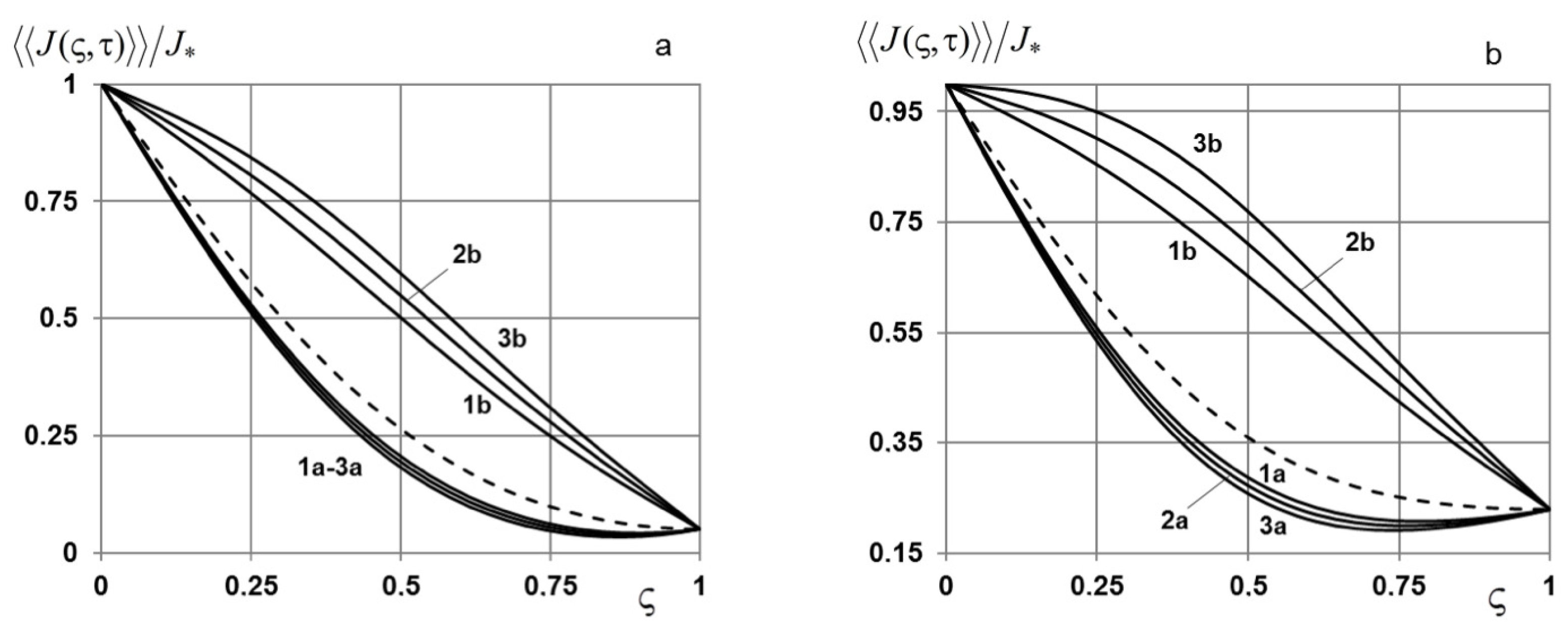We set the following basic parameters for the problem $\tau$ = 0.1; $c_{*}/J_{*}$ = 0.1; $D_1/D_0$ = 0.01 for a curves, and $D_1/D_0$ = 5 for b curves. In Figure 4, we have shown distributions of the averaged mass flows in the multilayered strip for different values of $h_{max}$ under fixed value $h_{min}$ for $n_1$ = 20 at zero initial admixture concentration (Figure 4a) and at non-zero constant concentration (Figure 4b). The 1 curves are built for the interval [0.01; 0.015], 2 curves for [0.01; 0.02], and 3 curves for [0.01; 0.025]. Dash lines represent the corresponding flows in the homogeneous strip of the matrix characteristics.

Figure 5 illustrates the behaviour of averaged mass flow at zero (Figure 5a) and at non-zero constant (Figure 5b) initial concentrations depending on number of inclusions whose thicknesses are of uniform distribution over the interval [0.01; 0.02]. Here curves 1–3 are built for $n_1$ = 5, 10, and 20, respectively.

Notice that the change in length of the interval of probable values of inclusion thickness $[h_{min};h_{max}]$ under a fixed value of one of its end points identically affects the values of function $〈〈J(\zeta ,\tau )〉〉/J_{*}$. In the case when the coefficients of diffusion in inclusions are greater than in matrix, the increase in $\Delta h$ at fixed $h_{min}$ leads to an increase in the flux (Figure 4). Herewith, in the case of non-zero initial concentration the larger the thickness value, the faster the flow function becomes convex up (curves 2b and 3b, Figure 4b). In the case where the coefficient of admixture diffusion in matrix is greater than in layers, the distinction between the values of the fluxes reaches maximum of 12% with the greatest band in the middle of the strip (a curves, Figure 4a).

The increase in the number of inclusions for $D_1<D_0$ at both zero and non-zero constant initial concentrations leads to a decrease in the averaged diffusion flux (a curves, Figure 5a). In the opposite case, the greater the number of inclusions $n_1$, the greater the function $〈〈J(\zeta ,\tau )〉〉/J_{*}$ differs from the flow in a homogeneous structure (b curves, Figure 5b). The increase in the length of the interval $[h_{min};h_{max}]$ in the vicinity of the same point does not affect values of the averaged flux (the difference being in the 5-th decimal place).

7.2. Numerical Analysis of Calculation of Averaged Diffusion Flows in Stratified Strip under Triangular Distribution of Inclusion Thickness

On the basis of the Formulae (38) and (39), we investigate dependence of the averaged flux on the interval of probable values of inclusion thickness and on the number of them. Calculation is performed in the dimensionless variables (41). Here, the basic values of the problem parameters are $\tau$ = 0.1; $c_{*}/J_{*}$ = 0.1; $D_1/D_0$ = 0.01 for a curves, and $D_1/D_0$ = 5 for b curves.

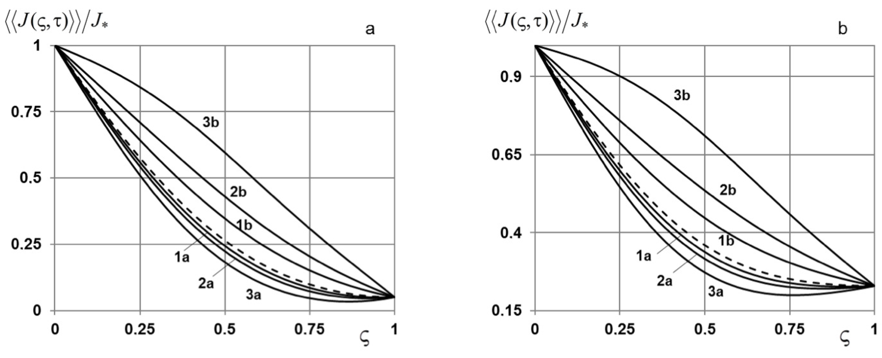
Figure 6 illustrates distributions of the averaged diffusion flow at zero (Figure 6a) and non-zero constant (Figure 6b) initial concentrations for different values of $\Delta h$ under the fixed maximal probable value of the inclusion thickness $h_{min}$ for $n_1$ = 10. Here, curves 1–3 were drawn for the same intervals of probable thickness as in Figure 4. Dash lines represent the flows in the strip without inclusions. In Figure 7, typical graphs of the averaged flows of admixture particles at zero (Figure 7a) and non-zero (Figure 7b) initial concentrations are shown for different values of inclusion thickness in the interval [0.01; 0.015]. Here the curves 1–3 correspond to the values of $n_1$ = 10, 20, and 30, respectively.

Like in the case of uniform distribution of the thickness of inclusions, the increase in the length of the interval of their probable values under a fixed value of one of interval end points for $D_1>D_0$ leads to an increase in the averaged mass flux (b curves, Figure 6). In the case of greater values of the diffusion coefficient in matrix than in inclusions, change in $\Delta h$ does not considerably affect the values and behaviour of the diffusion flow function. In particular, maximal difference between values reaches 5% in the vicinity of the middle of the strip (a curves, Figure 6). In this case, increasing the number of inclusions leads to decreasing the averaged flux both for zero and non-zero constant initial concentrations (a curves, Figure 7). At the same time, the increase in $n_1$ for $D_1>D_0$ leads to an increase in the mass flux (b curves, Figure 7). Additionally, for $n_1>$ 20, under given values of parameters of numerical investigation the function $〈〈J(\zeta ,\tau )〉〉/J_{*}$ becomes convex up (curve 3b, Figure 7).

Like in the previous cases, extension or narrowing of the interval of probable values of inclusion thickness in the vicinity of the same point of the coordinate axis almost does not affect the values of the function $〈〈J(\zeta ,\tau )〉〉/J_{*}$ (changes are in the 5-th decimal place). Moreover, the values of the averaged fluxes in a multilayered strip for uniform and triangular distributions of thickness of inclusions for $\tau >$0.05 coincide (the difference in the values are less than 1%).

8. Simulation of Averaged Flows of Admixture in Multilayered $\mathit{Fe}-\mathit{Cu}$ and $\mathit{\alpha }$$\mathit{Fe}-\mathit{Ni}$ Materials

Copper–steel bimetal composites are one of the most widely used composites which combines performances of the two metals and low cost [33]. However, modelling their diffusion properties to achieve optimal parameters also has an economic effect. Particularly, in the paper [34], an analytical model is developed to predict the mechanical strength of the copper matrix nanocomposite reinforced by steel particles in the spherical form.

Consider the problem of hydrogen diffusion in stratified composite $Fe-Cu$ material where iron is taken as a basic phase. According to [35,36], the coefficients of hydrogen diffusion are of $D_{Fe}=1.8·{10}^{-11}$ m${}^2$/s in iron, and of $D_{Cu}=4.34·{10}^{-10}$ m${}^2$/s in copper. Then, we obtain $D_1/D_0=D_{Cu}/D_{Fe}=24.11$.

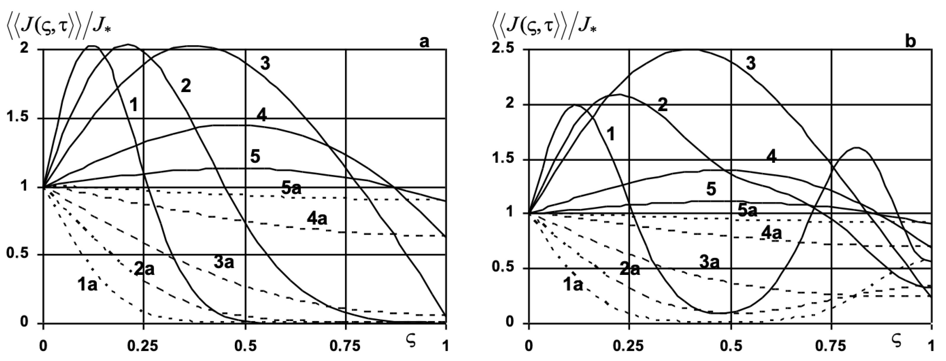
In Figure 8 there is shown the behaviour of the averaged diffusion flows of hydrogen at different instants of dimensionless time $\tau$=0.01; 0.03; 0.1; 0.5; 1 (curves 1–5, respectively) for zero (Figure 8a) and non-zero constant (Figure 8b) initial concentrations of H in the composite of $Fe-Cu$. We have assumed that number of copper inclusions in the iron layer is of $n_1$=20, the ratio $c_{*}/J_{*}$ of the initial concentration of hydrogen to its flux at the upper boundary of strip equals 0.1. 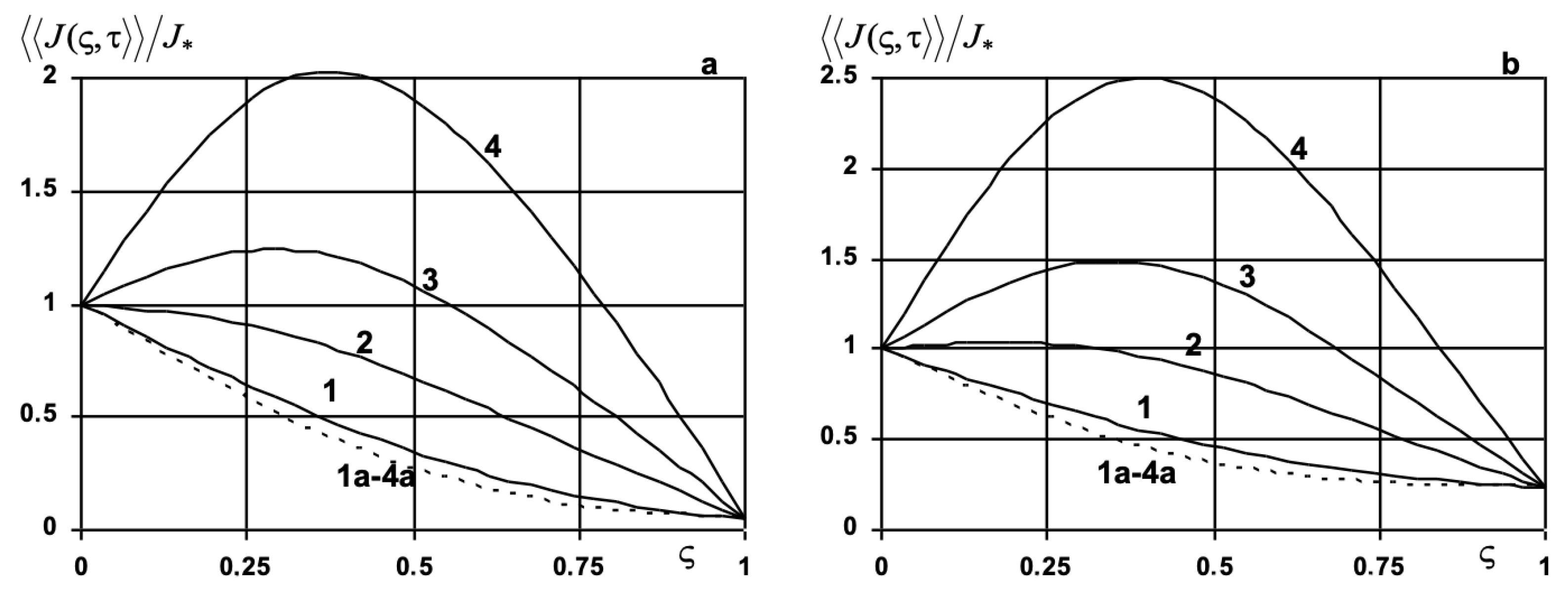Figure 9 demonstrates graphs of the averaged fluxes of hydrogen for different number of layers of $Cu$ in iron; for $n_1$= 1, 5, 10, and 20 (curves 1–4) at zero initial concentration H (Figure 9a) and for different values $c_{*}/J_{*}$ at non-zero constant initial concentration H (Figure 9b). In Figure 8 and Figure 9, a curves (dash) correspond the admixture fluxes in the homogeneous iron layer, b curves (full) correspond the fluxes in the iron strip with copper sublayers.

Occurrence of randomly disposed layers of copper in the iron layer leads to an increase in the averaged flows of hydrogen (Figure 8 and Figure 9). With this, the formation of near-surface maxima of fluxes in $Fe-Cu$ composite in the vicinity of the upper boundary of the body under zero initial concentration of hydrogen (Figure 8a) and in the vicinity of the upper and the lower boundaries under non-zero constant initial concentration (Figure 8b) is characteristic of small values of time. With time, the maximum of the function $〈〈J(\zeta ,\tau )〉〉/J_{*}$ in the vicinity of the upper boundary shifts to the middle of stratified structure (curve 3b, Figure 9b) and the maximum near the bottom boundary decreases (curve 2b, Figure 9b). Here, the difference between the flows of hydrogen in the homogeneous iron layer and in iron-copper composite decreases (curve 5b, Figure 8), and the flows of H reach linear dependence in steady-state regime.

The behaviour of the flow functions under the increase in the number of $Cu$ inclusions is the same for both zero and non-zero constant initial concentrations of hydrogen. Thus, the increase in the of number inclusions leads to an increase the hydrogen flux in $Fe-Cu$ composite (Figure 9a). Here, in the case of more than 8 copper layers the value of $〈〈J(\zeta ,\tau )〉〉/J_{*}$ becomes greater than the magnitude of flux at the upper body boundary (curves 3 and 4, Figure 9a). Raising the initial concentration of hydrogen leads to an increase in its averaged fluxes. The greatest value of this increase is observed in the middle of the $Fe-Cu$ strip (b curves, Figure 9b).

8.1. Simulation of Averaged Flow of Carbon in Stratified $\alpha Fe-Ni$ Material (Uniform Distribution of Inclusion Thickness)

Consider the diffusion of atoms of carbon in a stratified composite $\alpha$-iron-nickel material. Here, we also assume that iron is the basic phase. The coefficients of diffusion of carbon in iron and that in nickel are of $D_{\alpha Fe}=6.3·{10}^{-7}$ m${}^2$/s, $D_{Ni}=9·{10}^{-6}$ m${}^2$/s [35,36]. Then, we obtain $D_1/D_0=D_{Ni}/D_{\alpha Fe}=14.286$. Notice that the presence of atoms of carbon in the $\alpha Fe-Ni$ composite hardens its surface.

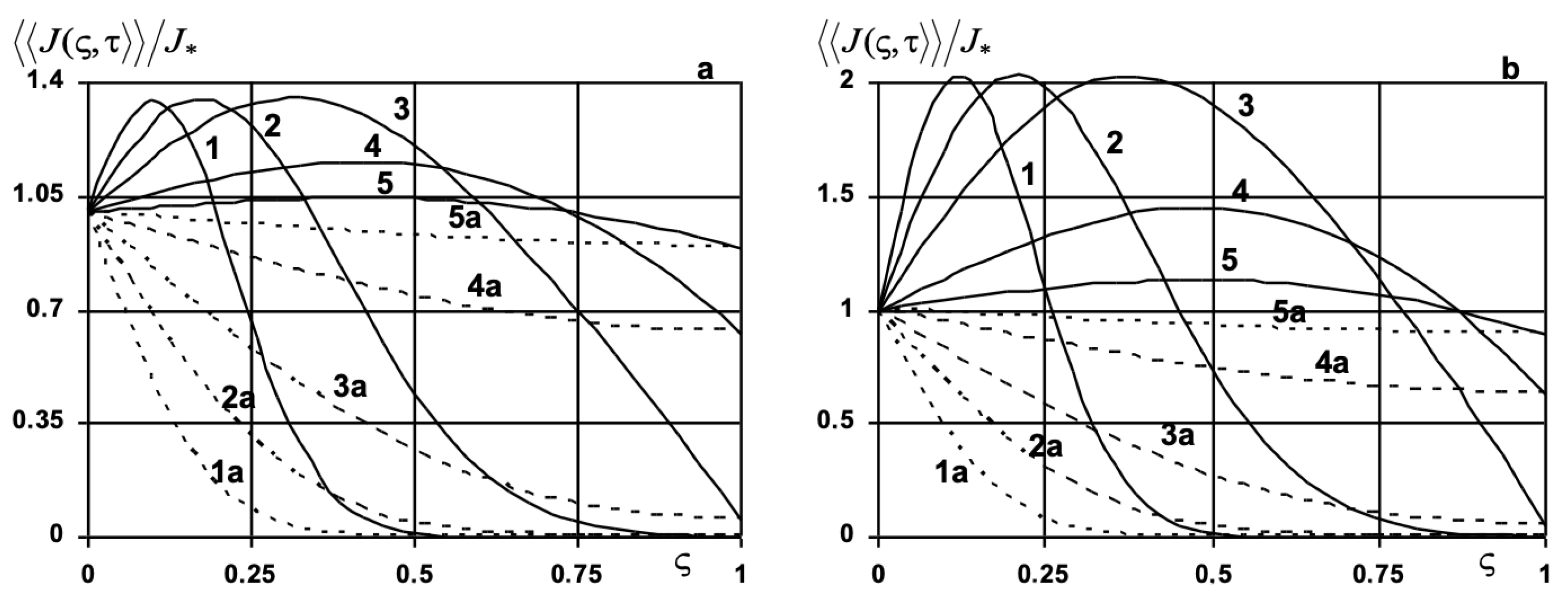
Figure 10 illustrates the behaviour of the averaged flows of carbon in different instants of dimensionless time $\tau$ = 0.01, 0.03, 0.1, 0.5, and 1 (curves 1–5, respectively) for zero (Figure 10a) and non-zero constant (Figure 10b) initial concentrations of C in the stratified $\alpha Fe-Ni$ material. The results of calculations are presented for 20 nickel layers for the volume fraction of nickel $v_{Ni}$ = 0.2 and the ratio of the initial concentration of carbon to its flux at the upper boundary $c_{*}/J_{*}$ = 0.1. We choose $h_{Ni}=0.01$ as the central point of the interval of probable values of sublayer thickness. In Figure 11a, the typical distributions of carbon for different values of minimal possible value of thickness of Ni inclusions in material $\alpha Fe-Ni$ at zero initial concentration are presented. Here, curves 1–4 correspond to the values $h_{min}$ = 0.001, 0.003, 0.005, and 0.01, respectively. Figure 11b illustrates behaviour of the averaged flows of carbon in $\alpha Fe-Ni$ composite at non-zero constant initial concentration for different values of $c_{*}/J_{*}$=0.01, 0.1, 0.2, 0.3, and 0.4 (curves 1–5, respectively) at the instant $\tau$ = 0.1. Figure 12 presents distributions of the averaged flows of admixture in $\alpha Fe-Ni$ composite at $h_{min}$ = 0.01, $h_{max}$ = 0.02 (Figure 12a) and $h_{min}$ = 0.02, $h_{max}$ = 0.03 (Figure 12b) for different instants of time $\tau$ = 0.01, 0.03, 0.05, 0.1, and 0.6. In Figure 10, Figure 11 and Figure 12, a curves (dash) corresponds to the admixture fluxes of carbon in the homogeneous $\alpha Fe$ layer, b curves (full) is plotted for the fluxes in the body with nickel layers.

Notice that presence of nickel sublayers in $\alpha Fe$ layer increases the carbon flux (Figure 10 and Figure 11). With this, the greatest distinction between the fluxes in homogeneous and in non-homogeneous strips is observed near the upper boundary of the body for zero initial value of concentration of carbon (curves 1b and 2b, Figure 10a) and vicinities of the upper and lower surfaces for non-zero constant distribution of C at the initial instant (curve 1b, Figure 10b). The aforesaid is characteristic only of small values of time. With increase in number of nickel inclusions the averaged flux of carbon also increases, and its value can be greater that the flux at the upper boundary of $\alpha Fe-Ni$ composite structure (curve 4, Figure 10b). The greater the value of initial concentration of carbon, the greater the difference between fluxes in the homogeneous and non-homogeneous strips (b curves, Figure 10b).

Comparison of Figure 12a,b gives us the opportunity to determine the effect of the shift of the interval of probable values of inclusion thickness when the length of the interval length remains the same. Thus, increase in probable values of the thickness can lead to the rise of the averaged flux and formation of a maximum of the function $〈〈J(\zeta ,\tau )〉〉$ near the body’s surface where the constant value $J_{*}$ of the flow is kept. With time, this maximum shifts to centre of the strip (Figure 12b).

8.2. Simulation of Averaged Flow of Hydrogen in Stratified $\alpha Fe-Ni$ Material (Triangular Distribution of Inclusion Thickness)

Consider diffusion process of atoms of hydrogen in the stratified $\alpha$-iron-nickel composite material. Here, we also assume that iron is the basic phase. The coefficients of diffusion of hydrogen in iron and in nickel are the following [35,36]: $D_{\alpha Fe}=6.42·{10}^{-8}$ m${}^2$/s, $D_{Ni}=9.5·{10}^{-7}$ m${}^2$/s. Then, we obtain $D_1/D_0=D_{Ni}/D_{\alpha Fe}$ = 14.797. In Figure 13, there is shown the behaviour of the averaged flows of hydrogen in different instants of dimensionless time, $\tau$= 0.01, 0.03, 0.1, 0.5, and 1 (curves 1–5, respectively) for zero (Figure 13a) and non-zero constant (Figure 13b) initial concentrations of H in the stratified $\alpha Fe-Ni$ composite. We have accepted that number of nickel inclusions in $\alpha$-iron layer is of $n_1$ = 20 for the volume fraction of nickel $v_{Ni}$ = 0.2, the ratio of the initial concentration of carbon to its flux at the upper boundary $c_{*}/J_{*}$ = 0.1. We choose $h_{Ni}^{min}$= 0.01 as the minimal value of the interval of probable values of layer thickness; and we have taken $\Delta h_{Ni}$ = 0.02. The a curves (dash) correspond to the mass fluxes of hydrogen in the homogeneous $\alpha Fe$ layer, the b curves (full) are plotted for the fluxes in the body with nickel layers. 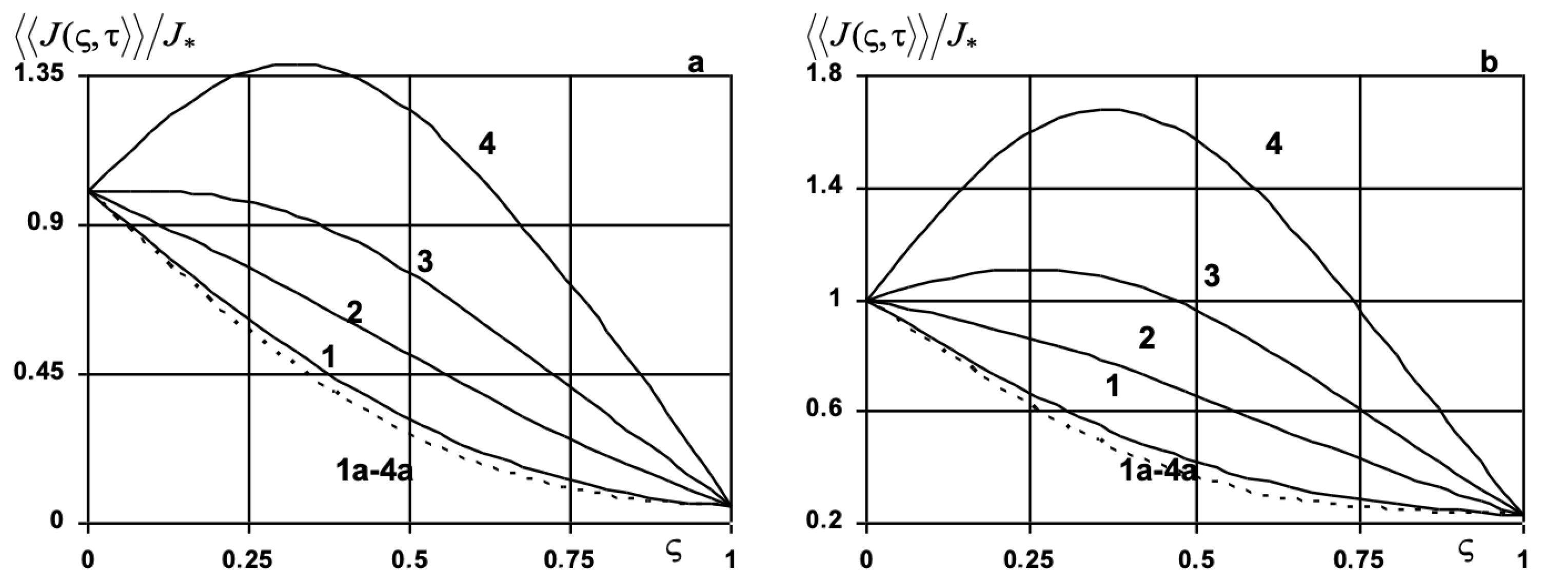Figure 14 presents distributions of the averaged fluxes of hydrogen for different numbers of nickel layers in $\alpha$-iron layer at zero (Figure 14a) and non-zero constant (Figure 14b) initial concentration of H at the instant of time $\tau$ = 0.1. The curves 1–4 correspond the values $n_1$ = 1, 5, 10, and 20. In Figure 15, there are shown distributions of the averaged fluxes of atoms of hydrogen in $\alpha Fe-Ni$ composite at $h_{min}$ = 0.01, $h_{max}$ = 0.02 (Figure 15a) and $h_{min}$ = 0.02, $h_{max}$ = 0.03 (Figure 15b) for different instants of time, $\tau$ = 0.01, 0.03, 0.05, 0.1, and 0.6. In Figure 13, Figure 14 and Figure 15, a curves (dash) corresponds to the admixture fluxes of carbon in the homogeneous $\alpha Fe$ layer, b curves (full) are plotted for the fluxes in the body with nickel layers.

The presence of atoms of hydrogen in $\alpha Fe-Ni$ composite at the initial instant of time increases values of the averaged fluxes (Figure 13b and Figure 14b). Moreover, the greater the number of nickel inclusions in iron layer, the more the flux of H differs from the flux in iron homogeneous body (Figure 14). Additionally, here, change in the thickness of Ni layers almost does not affect the value of function $〈〈J(\zeta ,\tau )〉〉/J_{*}$. Like in the case of $Fe-Cu$ composite, the increase in the initial concentration of hydrogen in stratified $\alpha Fe-Ni$ material leads to the rise of the averaged fluxes of C. The greatest increase is in the middle of the composite (Figure 14).

As in previous cases, a comparison of Figure 15a,b leads to the conclusion about the effect of shift of the interval of probable values of inclusion thickness when the length of the interval remains the same. Here, the increase probable values of the thickness can also lead to rise of the averaged flux, but the size of this increase is somewhat less. Notice that the maximum of the function $〈〈J(\zeta ,\tau )〉〉$ can become greater that the value $J_{*}$ at the upper boundary of the composite layer (Figure 15b).

9. Comparative Analysis of Solutions Depending on Stage of the Procedure of Averaging over Thickness

In the above-stated cases, the procedure of averaging the diffusion flows over random thickness of inclusions has been carried out after construction of the solution of initial-boundary value problem in the form of Neumann series and after averaging over the ensemble of phase configurations, i.e., this procedure is the last stage of solving the problem. Notice that if, at first, we average the flow over the random thickness and then over the ensemble of phase configurations, we obtain the same calculation formulae because the random variables with respect to which the averaging is carried out (i.e., the coordinates of inclusion location and inclusion thickness) are independent.

Let us consider the case of the procedure of averaging over the random thickness in the first stage, then construction of the solution in the form of Neumann series and averaging it over the ensemble of phase configurations for the example of the diffusion problem in the two-phase multilayered body at non-zero initial concentration and after this let us analyse the results of numerical experiments.

On the basis of the diffusion problem in the two-phase multilayered body at non-zero initial concentration let us consider the case when the procedure of averaging over the random thickness is carried out in the first stage of the problem solving. After that the construction of the solution in the form of Neumann series and averaging it over the ensemble of phase configurations are performed. Let us analyse the results of numerical experiments.

We average the thickness of inclusions, which is the random variable over the interval $[h_{min};h_{max}]$, as follows

$$〈h〉=\underset{h_{min}}{\overset{h_{max}}{\int }}h\tilde{f}\left(h\right)dh,$$

(42)

where $\tilde{f}\left(h\right)$ is the function of density of probable distribution.

In the case of uniform distribution of the inclusion thickness we have:

$$〈h〉=\overline{h}=(h_{max}-h_{min})/2.$$

(43)

If the thickness is of triangular distribution over the interval $[h_{min};h_{max}]$, then substituting the expression for distribution density into Relation (42) we obtain

$$〈h〉=4\overline{h}\Delta h^{-2}[h_{max}^2-h_{min}{h}_{max}+h_{min}^2-{\overline{h}}^2].$$

(44)

Then, for finding the averaged diffusion flux in the randomly non-homogeneous strip with layers of uniform or triangular distributions of thickness we use the previously obtained Expression (10), where we substitute the calculated according to (43) or (44) values of $〈h〉$ concerning the specific values of $h_{min}$ and of $h_{max}$ for the quantity $h_{i1}$. Thus, we obtain the expression for the diffusion flow under zero initial concentration

$$\frac{1}{J_{*}}{〈{〈J(z,t)〉}_{conf}〉}_h=1-\frac{2}{z_0}\sum _{n=1}^{\infty }\frac{1}{{\xi }_n}{e}^{-D_0{\xi }_n^{2}t}sin\left({\xi }_{n}z\right)+\frac{2v_1(D_1-D_0)n_1}{D_0{z}_0^2}\times$$

$$\times \sum _{k=1}^{\infty }\sum _{n=1}^{\infty }\frac{{\xi }_n{\overline{A}}_{kn}}{y_k^2-{\xi }_n^2}\left[e^{-D_0{\xi }_n^{2}t}-e^{-D_0{y}_k^{2}t}\right]sin\left(y_{k}z\right)$$

(45)

and under non-zero constant initial concentration of admixture

$$\frac{1}{J_{*}}{〈{〈J(z,t)〉}_{conf}〉}_h=1-\frac{2}{z_0}\sum _{n=1}^{\infty }{e}^{-D_0{\xi }_n^{2}t}\left(\frac{1}{{\xi }_n}+{(-1)}^n\frac{D_0{c}_{*}}{J_{*}}\right)sin\left({\xi }_{n}z\right)+$$

$$+\frac{2v_1(D_1-D_0)}{D_0{z}_0^2}\sum _{k=1}^{\infty }\sum _{n=1}^{\infty }\frac{{\xi }_n{\overline{A}}_{kn}}{y_k^2-{\xi }_n^2}\left(1+{(-1)}^n\frac{D_0{c}_{*}}{J_{*}}{\xi }_n\right)\times$$

$$\times \left[e^{-D_0{\xi }_n^{2}t}-e^{-D_0{y}_k^{2}t}\right]sin\left(y_{k}z\right).$$

(46)

Here ${\overline{A}}_{kn}=\frac{cos\left[(y_k-{\xi }_n)〈h〉\right]}{〈h〉{(y_k-{\xi }_n)}^2}-\frac{cos\left[(y_k+{\xi }_n)〈h〉\right]}{〈h〉{(y_k+{\xi }_n)}^2}-\frac{4y_k{\xi }_n}{〈h〉{(y_k^2-{\xi }_n^2)}^2}+{(-1)}^{k+n}\frac{2y_k}{y_k^2-{\xi }_n^2}$.

Notice that in the expressions (45) and (42), which have been obtained with the use of averaging the inclusion thickness at the first stage of the problem solving, parts of solutions which take into account the influence of non-homogeneities of body’s structure directly proportional to the volume fraction of inclusions $v_1$ ($v_1=n_1〈h〉/z_0$).

Table 1. Calculating data for the averaged flows under uniform distribution of the inclusion thickness at nonzero constant initial concentration of admixture.

$\mathit{\zeta }$	${〈{〈{\mathit{J}}_1〉}_{\mathit{h}}〉}_{\mathit{conf}}$	${〈{\mathit{J}}_1\left(〈\mathit{h}〉\right)〉}_{\mathit{conf}}$	${〈{〈{\mathit{J}}_2〉}_{\mathit{h}}〉}_{\mathit{conf}}$	${〈{\mathit{J}}_2\left(〈\mathit{h}〉\right)〉}_{\mathit{conf}}$
0	1.000000	1.000000	1.000000	1.000000
0.0323	0.969299	0.978974	0.940184	0.940157
0.0968	0.861141	0.881994	0.822360	0.822281
0.1613	0.656076	0.680903	0.709846	0.709716
0.2258	0.412495	0.430423	0.605756	0.605582
0.2903	0.217320	0.218893	0.512427	0.512406
0.3548	0.096912	0.090091	0.431995	0.431972
0.4194	0.044126	0.033308	0.365259	0.365233
0.4839	0.042033	0.026401	0.312333	0.312308
0.5484	0.086542	0.071581	0.272581	0.272552
0.6129	0.216030	0.206562	0.244716	0.244688
0.6774	0.476667	0.475088	0.227028	0.227002
0.7419	0.845942	0.852242	0.217588	0.217565
0.8065	1.163142	1.186505	0.214630	0.214473
0.8710	1.274118	1.299927	0.216180	0.216072
0.9355	1.185859	1.205645	0.221207	0.221153
1	1.128379	1.128379	0.229091	0.229091

and

Table 2. Calculating data for the averaged flows under triangular distribution of the inclusion thickness at nonzero constant initial concentration of admixture.

$\mathit{\zeta }$	${〈{〈{\mathit{J}}_1〉}_{\mathit{h}}〉}_{\mathit{conf}}$	${〈{\mathit{J}}_1\left(〈\mathit{h}〉\right)〉}_{\mathit{conf}}$	${〈{〈{\mathit{J}}_2〉}_{\mathit{h}}〉}_{\mathit{conf}}$	${〈{\mathit{J}}_2\left(〈\mathit{h}〉\right)〉}_{\mathit{conf}}$
0	1.000000	1.000000	1.000000	1.000000
0.0323	0.968300	0.978974	0.940184	0.940157
0.0968	0.861537	0.881994	0.822360	0.822281
0.1613	0.662167	0.680903	0.709846	0.709716
0.2258	0.419055	0.430423	0.605756	0.605582
0.2903	0.211705	0.218893	0.512618	0.512406
0.3548	0.088722	0.090091	0.431995	0.431972
0.4194	0.030927	0.033308	0.365259	0.365233
0.4839	0.024645	0.026401	0.312333	0.312308
0.5484	0.070131	0.071581	0.272581	0.272552
0.6129	0.206819	0.206562	0.244716	0.244688
0.6774	0.469015	0.475088	0.227232	0.227002
0.7419	0.837423	0.852242	0.217763	0.217565
0.8065	1.167348	1.186505	0.214630	0.214473
0.8710	1.274651	1.299927	0.216179	0.216072
0.9355	1.179412	1.205645	0.221207	0.221153
1	1.128379	1.128379	0.229091	0.229091

show the calculation data for the averaged flux which have been calculated for the last stage of thickness averaging ${〈{〈J〉}_h〉}_{conf}$ and those with the first stage of thickness averaging ${〈J\left(〈h〉\right)〉}_{conf}$ for the first set of instants (marked with subindex 1): $\tau$ = 0.01; $D_1/D_0$ = 5; $c_{*}/J_{*}$ = 0.2; $v_1$ = 0.45; $h_{min}$ = 0.005; $h_{max}$ = 0.01 and the second set of instants (marked with subindex 2): $\tau$ = 0.1; $D_1/D_0$ = 0.01; $c_{*}/J_{*}$ = 0.1; $v_1$ = 0.2; $h_{min}$ = 0.005; and $h_{max}$ = 0.015. The data in Table 1 are calculated according to the Formulae (31) and (46), where $〈h〉$ is determined according to the Formula (43) in the case of uniform distribution of the layer thickness. The data in Table 2 are calculated according to (40) and (46), where $〈h〉$ is determined according to the Formula (44) in the case of triangular distribution of the inclusion thickness. Calculations were carried out in the dimensionless variables (41). Partition of the interval is made with the step $\Delta \zeta \approx$ 0.0323.

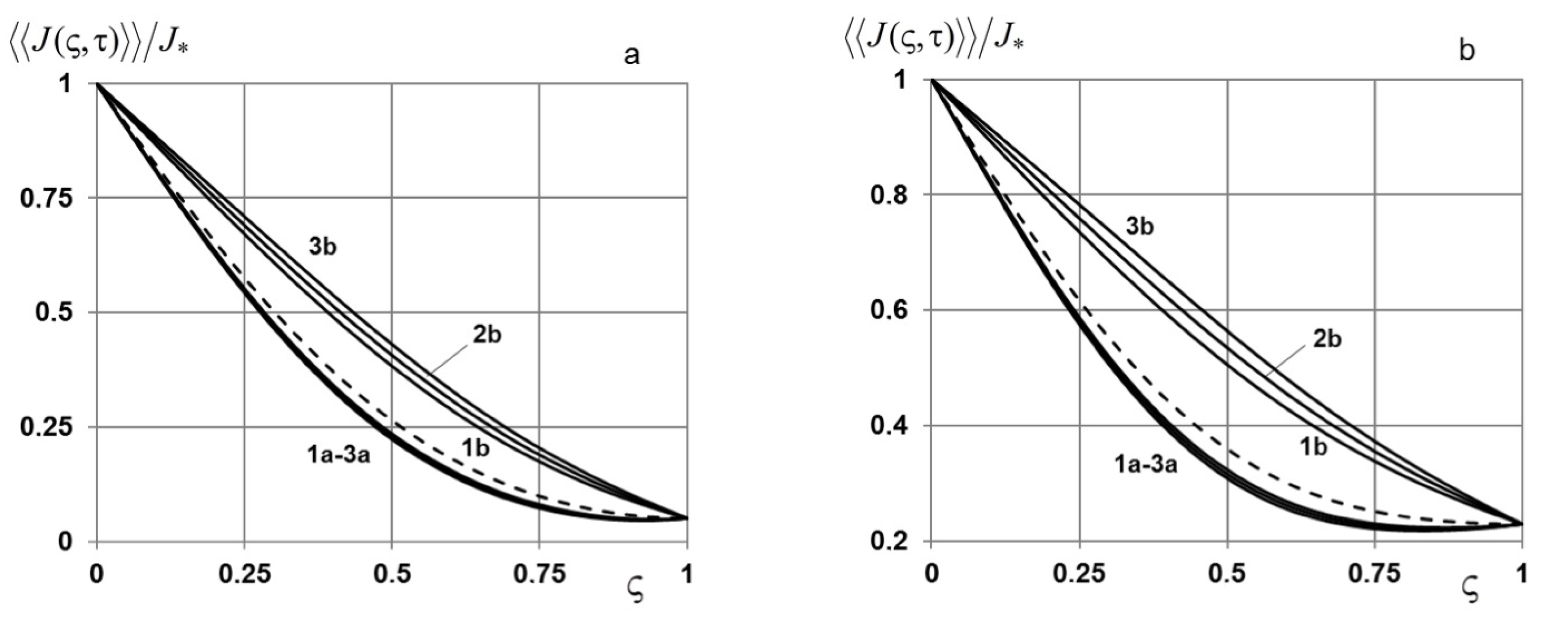
Figure 16 illustrates averaged diffusion flows for model problem of diffusion with the first stage of thickness averaging (a curves) and for model in which this procedure is the last stage of solving the problem (b curves). The 1 curves are plotted for the first set of instants and b curves are determined for the second set of instants.

Note that the difference between values of diffusion flows averaged over the inclusion thickness on the first and last stages are differentiated less that 1% (2 curves, Figure 16). However, for $\tau \le$ 0.01; $D_1/D_0>$ 1 and $v_1>$ 0.3 the difference between the flows can reach yet 2 significant digit (Table 1 and Table 2; 1 curves, Figure 16).

10. Conclusions

All obtained results are new. On the basis of the original approach, we have studied flows of admixture substance in two-phase stochastically non-homogeneous multi-layered strips with uniform distributions of non-homogeneities in body domain. With that the thickness of layered inclusions are the random variable with uniform or triangular distributions in the interval of its probable values. Within the scope of this approach the initial-boundary value problems are directly formulated for the functions of mass flow, the boundary conditions on one of the body surfaces are imposed for the function of mass flow and the conditions on admixture concentration are given on another boundary. Having considered the presence of stochastic non-homogeneities as internal sources, the initial-boundary value problem with random coefficients was reduced to the equivalent integro-differentual equation. Its solution was constructed by the method of successive iterations in the form of convergent Neumann series.

The calculating formulae for the averaged flow were obtained in the cases of zero and non-zero initial concentration of admixture. On this basis we have developed the program modules for qualitative and quantitative analysis of dependence of the averaged flow on such medium characteristics as the ratio of diffusion coefficients, the volume fraction of inclusions, etc. We carried out comparative analysis of the mass flows averaged over the random thickness during formation of the mathematical model and in the last stage of investigation.

It is important to note that taking into consideration of stochasticity of inclusion thickness depends on the values and/or behaviour of the averaged mass flow. So, in the case of larger values of the coefficient of admixture diffusion in inclusions than in matrix, shift of interval of probable values of inclusion thickness up to 1 leads to increasing the diffusion flow. For times of running the diffusion process being close to steady-state, difference between the values of averaged diffusion flows in the stratified layer for uniform and triangular distributions inclusion thickness is less than 1%. At the same time in the case of three-layered strip choice of type of distribution is essential. In both cases of the thickness distributions increasing the length of the interval of probable values of the inclusion thickness, the fixation of one of its ends leads to growth of the averaged flow of admixture. Obtaining such results is important for simplifying calculations in the study of mass flows in more complex structures, when averaging over thickness at the last stage of obtaining a solution can be difficult.

The proposed mathematical model and obtained calculation formulae can be used in the creation of layered composite materials. For example, the presence of hydrogen atoms in the body makes $\alpha Fe-Ni$ composite lighter, but more brittle. At the same time, the presence of more nickel layers in the body increases the diffusion flow of hydrogen compared to the iron layer. At the same time, the probability distribution of the thickness of these layers has almost no effect on achieving the goal. Therefore, during the technological process of manufacturing the composite, it is not necessary to achieve high accuracy in the dimensions of layered inclusions. However, the purpose of research may be the opposite. Additionally, notice that in order to use the obtained calculation formulae in engineering practice, it is necessary to know the diffusion coefficients of the migrating admixture for each material that constructing the body, the numerical data of the concentration of the admixture on the surface and its diffusion flow, which are experimentally measured values, as well as the number of layers and/or volume fraction of inclusions. In addition, it is necessary to establish or make assumptions about the probability distributions of random variables.

The practical significance of the obtained results is based on the need to take into account the presence of inclusions during the manufacture of composites, industrial adsorbents, and membranes, since the presence of inclusions in the medium affects the chemical reactivity and physical interaction of solids. The analysis and control of the properties of mass transfer in such media is carried out primarily by means of computer simulation and plays an important role in the design and evaluation of the effectiveness of the use of multilayered materials in various fields of engineering practice.

References

- Chen, C.; Chen, L.; Chen, S.; Yu, Y.; Weng, D.; Mahmood, A.; Wang, G.; Wang, J. Preparation of underwater superoleophobic membranes via TiO2 electrostatic self-assembly for separation of stratified oil/water mixtures and emulsions. J. Membr. Sci. 2020, 602, 117976. [Google Scholar] [CrossRef]
- Wang, Y.; Nie, Y.; Chen, C.; Zhao, N.; Zhao, Y.; Jia, Y.; Li, J.; Li, Z. Preparation and Characterization of a Thin-Film Composite Membrane Modified by MXene Nano-Sheets. Membranes 2022, 12, 368. [Google Scholar] [CrossRef] [PubMed]
- Hanebuth, M.; Dittmeyer, R.; Mabande, G.T. P.; Schwieger, W. On the combination of different transport mechanisms for the simulation of steady-state mass transfer through composite systems using H2/SF6 permeation through stainless steel supported silicalite-1 membranes as a model system. Catal. Today 2005, 104, 352–359. [Google Scholar] [CrossRef]
- Yu, Y. T.; Pochiraju, K. Three-Dimensional Simulation of Moisture Diffusion in Polymer Composite Materials. Polym.-Plast. Technol. Eng. 2003, 42, 737–756. [Google Scholar] [CrossRef]
- Ma, S.; Xing, F.; Deng, C.; Zhang, L. A novel analytical approach to describe the simultaneous diffusional growth of multilayer stoichiometric compounds in binary reactive diffusion couples. Script. Mater. 2021, 191, 111–115. [Google Scholar] [CrossRef]
- Panico, S.; Larcher, M.; Troi, A.; Baglivo, C.; Congedo, P.M. Thermal Modeling of a Historical Building Wall: Using Long-Term Monitoring Data to Understand the Reliability and the Robustness of Numerical Simulations. Buildings 2022, 12, 1258. [Google Scholar] [CrossRef]
- Beck, F.R.; Mohanta, L.; Henderson, D.M.; Cheung, F.-B.; Talmage, G. An engineering stability technique for unsteady, two-phase flows with heat and mass transfer. Int. J. Multiphase Flow 2021, 142, 103709. [Google Scholar] [CrossRef]
- Khoroshun, L.P. Mathematical Models and Methods of the Mechanics of Stochastic Composites. Int. Appl. Mech. 2000, 36, 30–62. [Google Scholar] [CrossRef]
- Bergins, C.; Crone, S.; Strauss, K. Multiphase Flow in Porous Media with Phase Change. Part II: Analytical Solutions and Experimental Verification for Constant Pressure Stream Injection. Transp. Porous Media 2005, 60, 275–300. [Google Scholar] [CrossRef]
- Schulenberg, T.; Muller, U. An improved model for two-phase flow through beds of coarse particles. Int. J. Multiphase Flow 1987, 13, 87–97. [Google Scholar] [CrossRef]
- Khoroshun, L.P.; Soltanov, N.S. Thermoelasticity of Two-Component Mixtures; Naukova Dumka: Kyiv, Ukraine, 1984. [Google Scholar]
- Mechkour, H. Two-Scale Homogenization of Piezoelectric Perforated Structures. Mathematics 2022, 10, 1455. [Google Scholar] [CrossRef]
- Poddar, N.; Saha, G.; Dhar, S.; Mondal, K.K. On solute dispersion in an oscillatory magneto-hydrodynamics porous medium flow under the effect of heterogeneous and bulk chemical reaction. Phys. Fluids 2022, 34, 1603. [Google Scholar] [CrossRef]
- Amosov, A.; Krymov, N. On a Nonlinear Initial—Boundary Value Problem with Venttsel Type Boundary Conditions Arizing in Homogenization of Complex Heat Transfer Problems. Mathematics 2022, 10, 1890. [Google Scholar] [CrossRef]
- Raveendran, V.; Cirillo, E.N.M.; de Bonis, I.; Muntean, A. Scaling effects on the periodic homogenization of a reaction-diffusion-convection problem posed in homogeneous domains connected by a thin composite layer. arXiv 2021, arXiv:2107.08448. [Google Scholar] [CrossRef]
- Lidzba, D.; Shao, J.S. Study of poroelasticity material coefficients as response of microstructure. In Mechanics of Cohasive-Fractional Materials; Wiley: Hoboken, NJ, USA, 2000. [Google Scholar] [CrossRef]
- Matysiak, S.; Mieszkowski, R. On homogenization of diffusion processes in microperiodic stratified bodies. Int. J. Heat Mass Transf. 1999, 26, 539–547. [Google Scholar] [CrossRef]
- Bonelli, S. Approximate solution to the diffusion equation and its application to seepage-related problems. Appl. Mat. Model. 2009, 2009 33, 110–126. [Google Scholar] [CrossRef]
- Eliáš, J.; Yin, H.; Cusatis, G. Homogenization of discrete diffusion models by asymptotic expansion. Int. J. Numer. Analyt. Methods Geomech. 2022, 1–22. [Google Scholar] [CrossRef]
- Eliáš, J.; Vořechovský, M. Fracture in random quasibrittle media: I. Discrete mesoscale simulations of load capacity and fracture process zone. Eng. Fract. Mech. 2020, 235, 107160. [Google Scholar] [CrossRef]
- Keller, J.B. Flow in Random Porous Media. Transp. Porous Media 2001, 43, 395–406. [Google Scholar] [CrossRef]
- Chernukha, O.Y.; Chuchvara, A.E. Modeling of the flows of admixtures in a random layered strip with probable arrangement of inclusions near the boundaries of the body. J. Math. Sci. 2019, 238, 116–128. [Google Scholar] [CrossRef]
- Chaplya, Y.; Chernukha, O.; Davydok, A. Mathematical modeling diffusion fluxes in randomly nonhomogeneous stratified strip. Rep. Natl. Acad. Sci. Ukr. 2012, 11, 40–46. [Google Scholar]
- Gyarmati, I. Non-Equilibrium Thermodynamics: Field Theory and Variational Principles; Springer: Berlin/Heidelberg, Germany, 1970. [Google Scholar]
- Crank, J.C. The Mathematics of Diffusion; Clarendon Press: Oxford, UK, 1975. [Google Scholar]
- Münster, A. Chemical Thermodynamics; Editorial URSS: Moscow, Russia, 2002. [Google Scholar]
- Burak, Y.Y.; Chaplya, Y.Y.; Chernukha, O.Y. Continuum-Thermodynamic Models of the Mechanics of Solid Solutions; Naukova Dumka: Kyiv, Ukraine, 2006. [Google Scholar]
- Rytov, S.; Kravtsov, Y.; Tatarskii, V. Principles of Statistical Radiophysics 1 Elements of Random Process Theory; Springer: Berlin/Heidelberg, Germany, 1987. [Google Scholar]
- Lykov, A.V. Theory of Thermal Conductivity; Higher School of Moscow: Moscow, Russia, 1987. [Google Scholar]
- Polyanin, A.; Manzhirov, A. Handbook of Integral Equations; Chapman and Hall/CRC: Boca Raton, FL, USA, 2008. [Google Scholar]
- Bilushchak, Y.; Goncharuk, V.; Chaplya, Y.; Chernukha, O. Mathematical modeling diffusion of admixture components under their cascade decay. Mater. Mach. Syst. 2015, 1, 146–155. [Google Scholar]
- Lykov, A. Theory of Heat Conduction; GTTI: Moscow, Russia, 1952. [Google Scholar]
- Wang, Y.; Gao, Y.; Li, Y. Review of preparation and application of copper–steel bimetal composites. Emerg. Mater. Res. 2019, 8, 538–551. [Google Scholar] [CrossRef]
- Norouzifard, V.; Naeinzadeh, H.; Talebi, A. Fabrication and investigation of mechanical properties of copper matrix nanocomposite reinforced by steel particle. J. Alloys Compounds 2021, 887, 161434. [Google Scholar] [CrossRef]
- Lavrik, V.; Filchakova, V.; Yashin, A. Conformal Mappings of Physico-Topological Models; Naukova Dumka: Kyiv, Ukraine, 2009. [Google Scholar]
- Dumitrescu, A.; Slatineanu, T.; Poiata, A.; Iordan, A.; Mihailescu, C.; Palamaru, M. Advanced composite materials based on hydrogels and ferrites for potential biomedical applications. Colloids Surf. A Physicochem. Eng. Aspects 2014, 455, 185–194. [Google Scholar] [CrossRef]
Figure 1.
Possible realization of a stratified strip (a) and schematic distribution of random thickness of inclusion in the interval (b).
Figure 2.
Schematic distribution of initial concentration in a two-phase stratified body.
Figure 3.
Function of density of triangular distribution for different values (a) and different values about point h = 0.22 (b).
Figure 4.
Averaged mass flows in the strip for different values of under fixed value at zero (a) and non-zero (b) initial concentrations.
Figure 5.
Averaged mass flows for different numbers of inclusions at zero (a) and non-zero (b) initial concentrations.
Figure 6.
Averaged mass flows at zero (a) and non-zero (b) initial concentration for different values of under fixed value .
Figure 7.
Averaged mass flows at zero (a) and non-zero (b) initial concentration for different number of inclusions in the body.
Figure 8.
Distributions of hydrogen flows in composite at zero (a) and non-zero constant (b) initial concentration in different instants.
Figure 9.
Distributions of hydrogen flows in composite for different numbers of copper inclusions at zero initial concentration (a) and different values at non-zero initial concentration (b).
Figure 10.
Distributions of carbon flows in composite at zero (a) and non-zero (b) initial concentrations for different instants .
Figure 11.
Distributions of carbon flows in composite at zero initial concentration for different values of minimal possible value of thickness of Ni inclusions in material (a) and for different values at non-zero constant initial concentration (b).
Figure 12.
Distributions of carbon flows in composite at zero initial concentration at , (a) and , (b) for different instants .
Figure 13.
Distributions of hydrogen flows in composite at zero (a) and non-zero constant (b) initial concentrations in different instants .
Figure 14.
Distribution of hydrogen flows in composite at zero (a) and non-zero constant (b) initial concentrations for different numbers of nickel inclusions.
Figure 15.
Distributions of hydrogen flows in composite at zero initial concentration at , (a) and , (b) for different instants .
Figure 16.
Comparison of two models of averaging over the inclusion thickness for structure with uniform (a) and triangular (b) distributions of the inclusions thickness.