


The Greatest Common Decision Maker: A Novel Conflict and Consensus Analysis Compared with Other Voting Procedures
 , and
, and 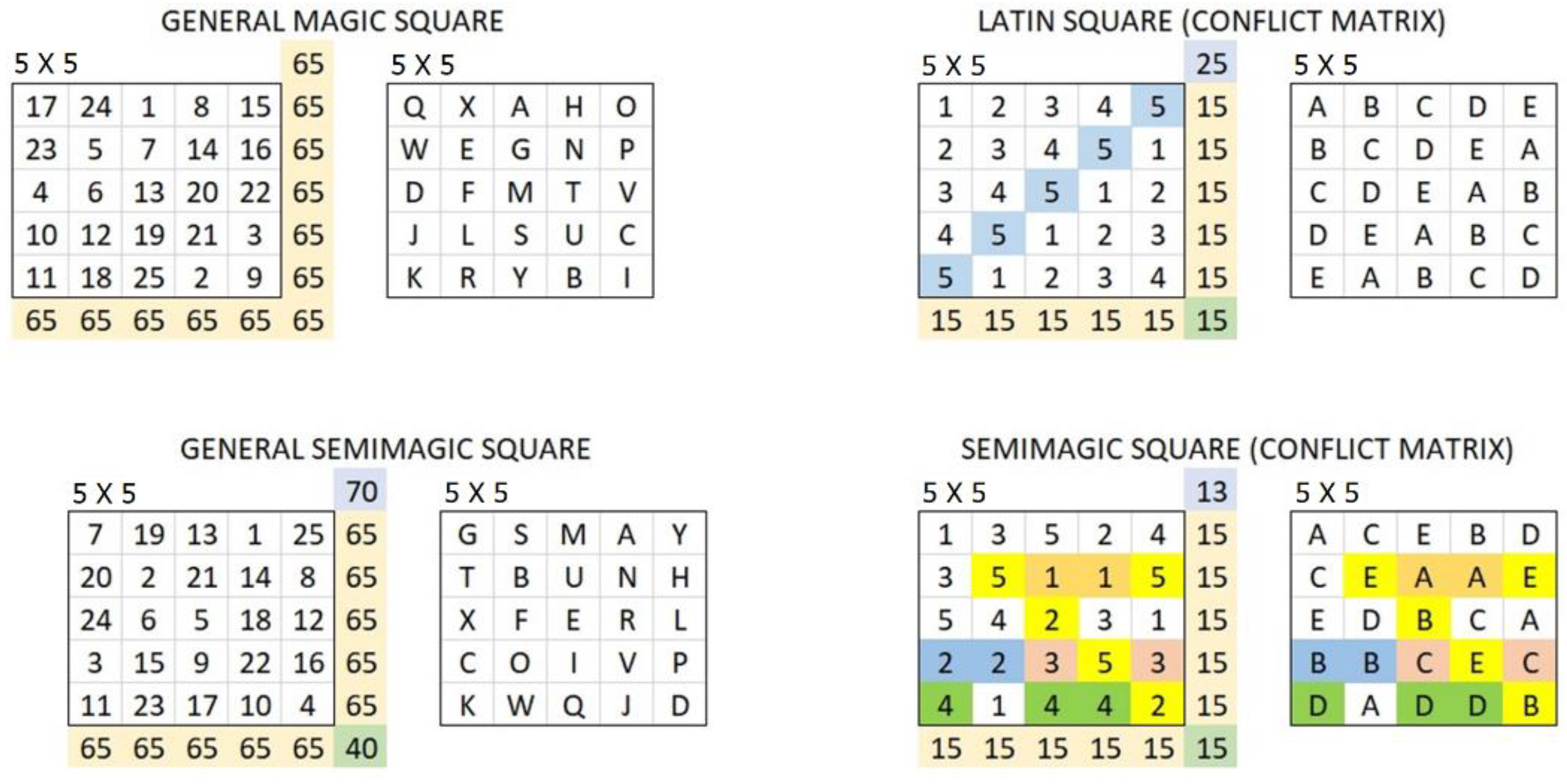
Abstract
:1. Introduction
Main Idea
2. Problem Statement
- How, in negotiation among agents or groups, can we help them reach a consensus, avoiding conflict among them? If each one does not know what the others think when deciding or choosing an alternative, is it possible to build an aggregation function that leads most of the cases to consensus rather than to partial or total conflict?
- In self-controlled groups where there is no moderator who reconciles a solution to conflicts, is it possible to get out of a conflict by visualizing the advantages or disadvantages of changing decisions at a certain cost?
3. Assumptions
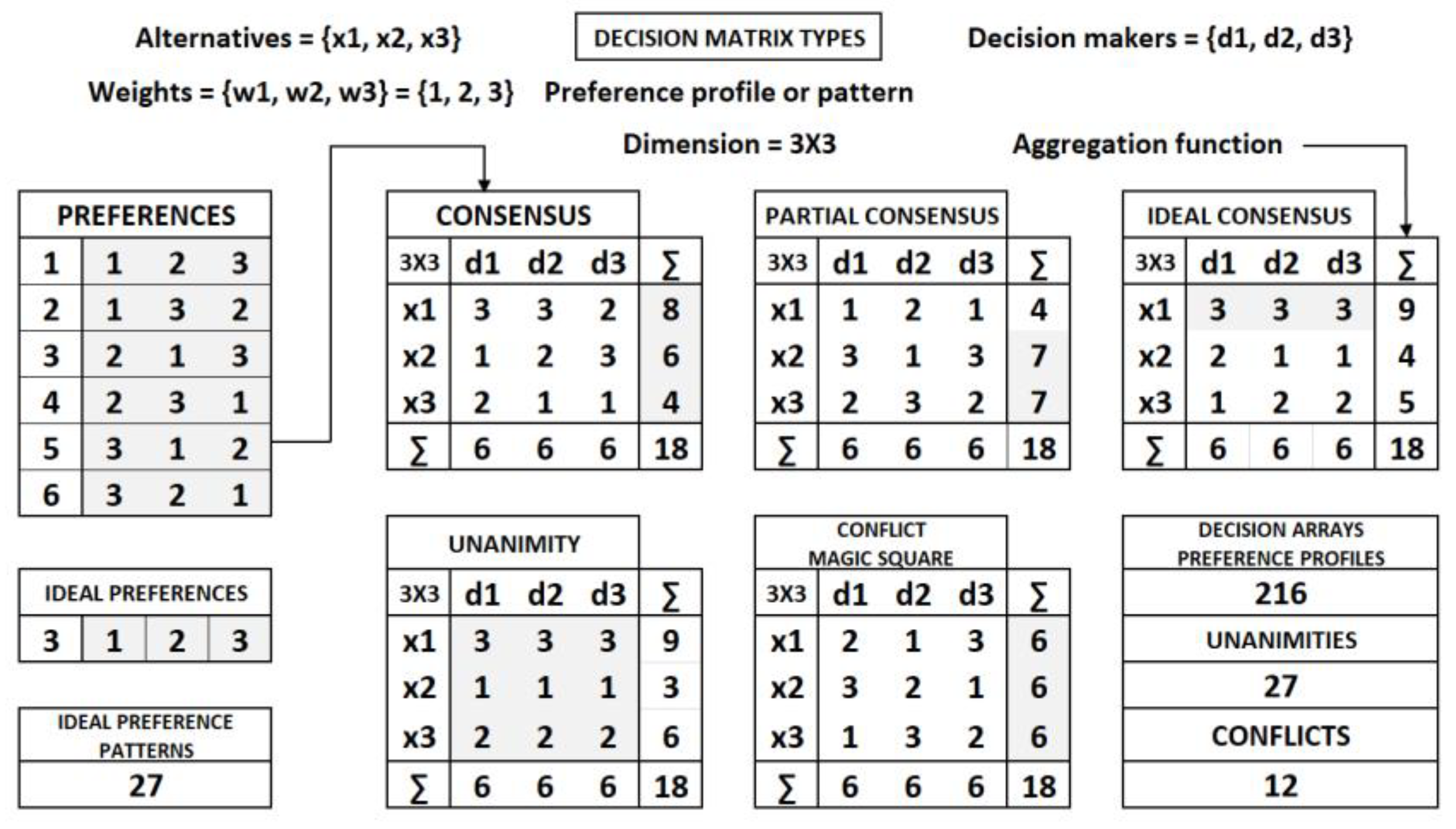
4. Concepts and Definitions
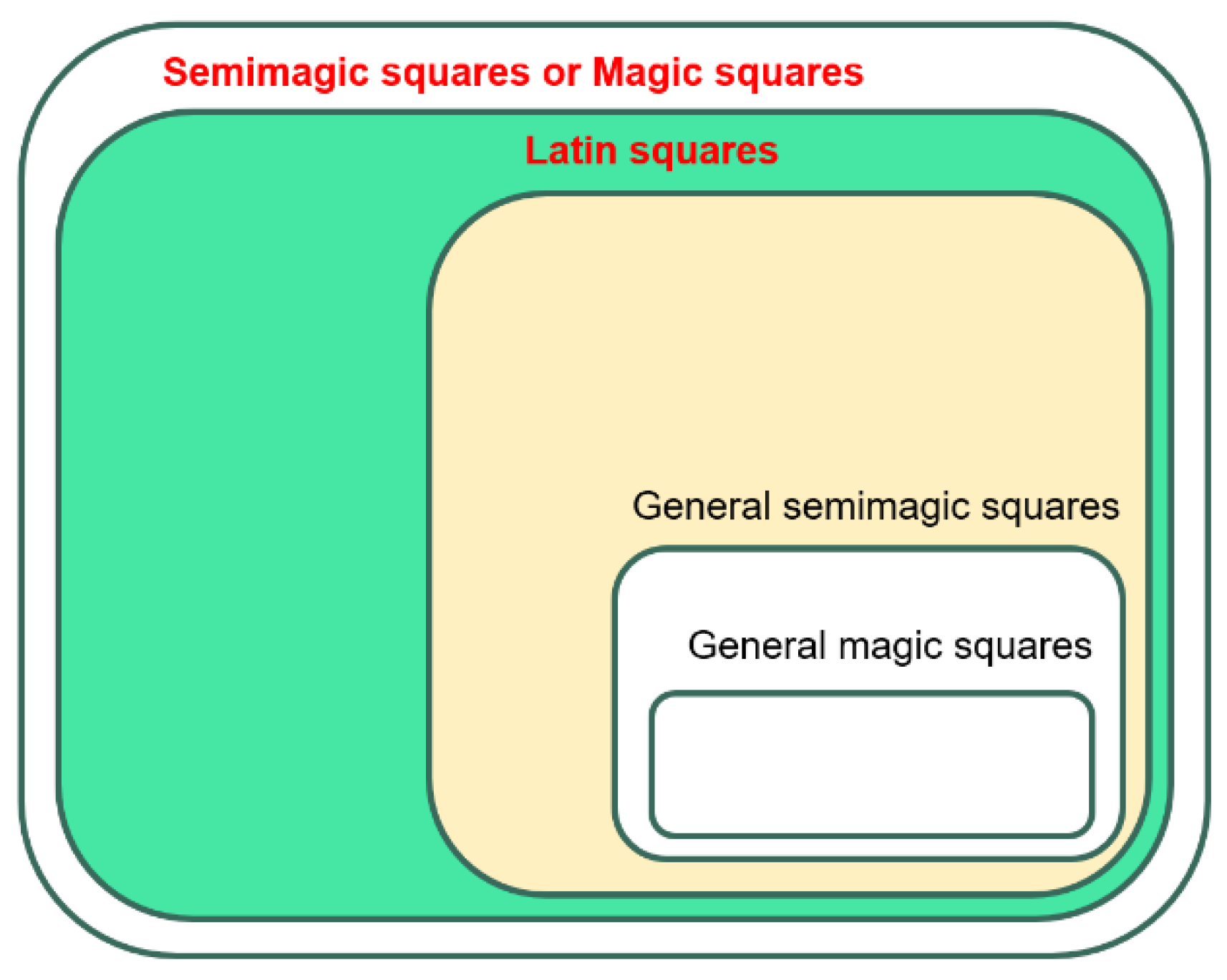
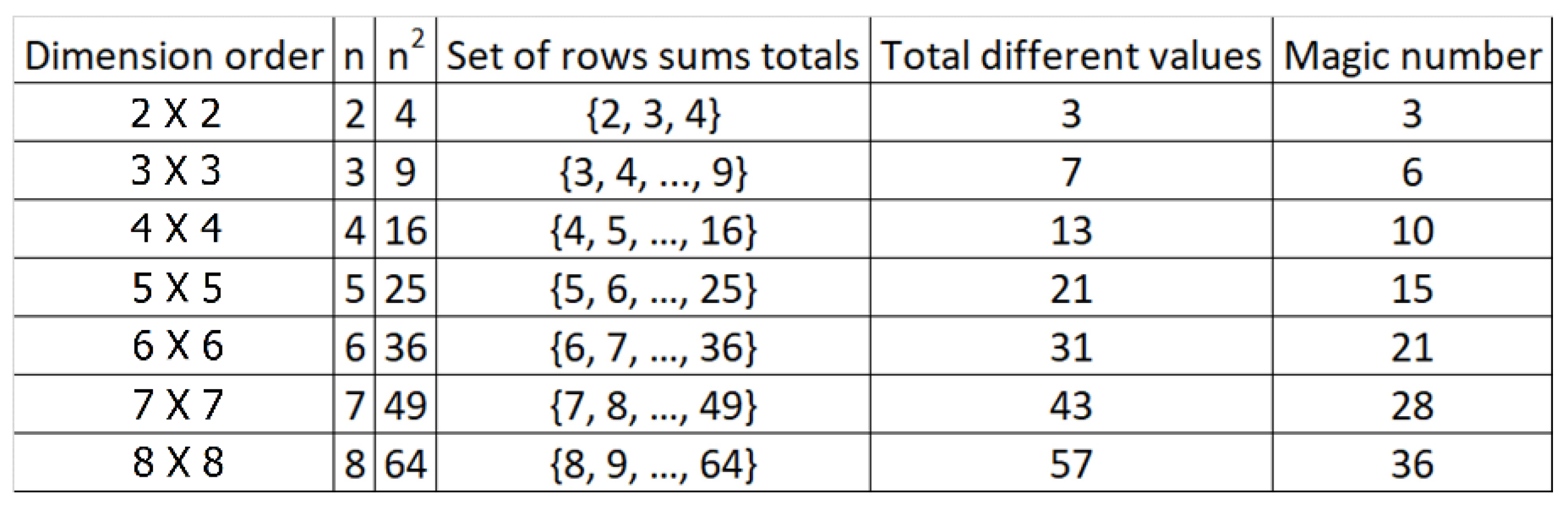
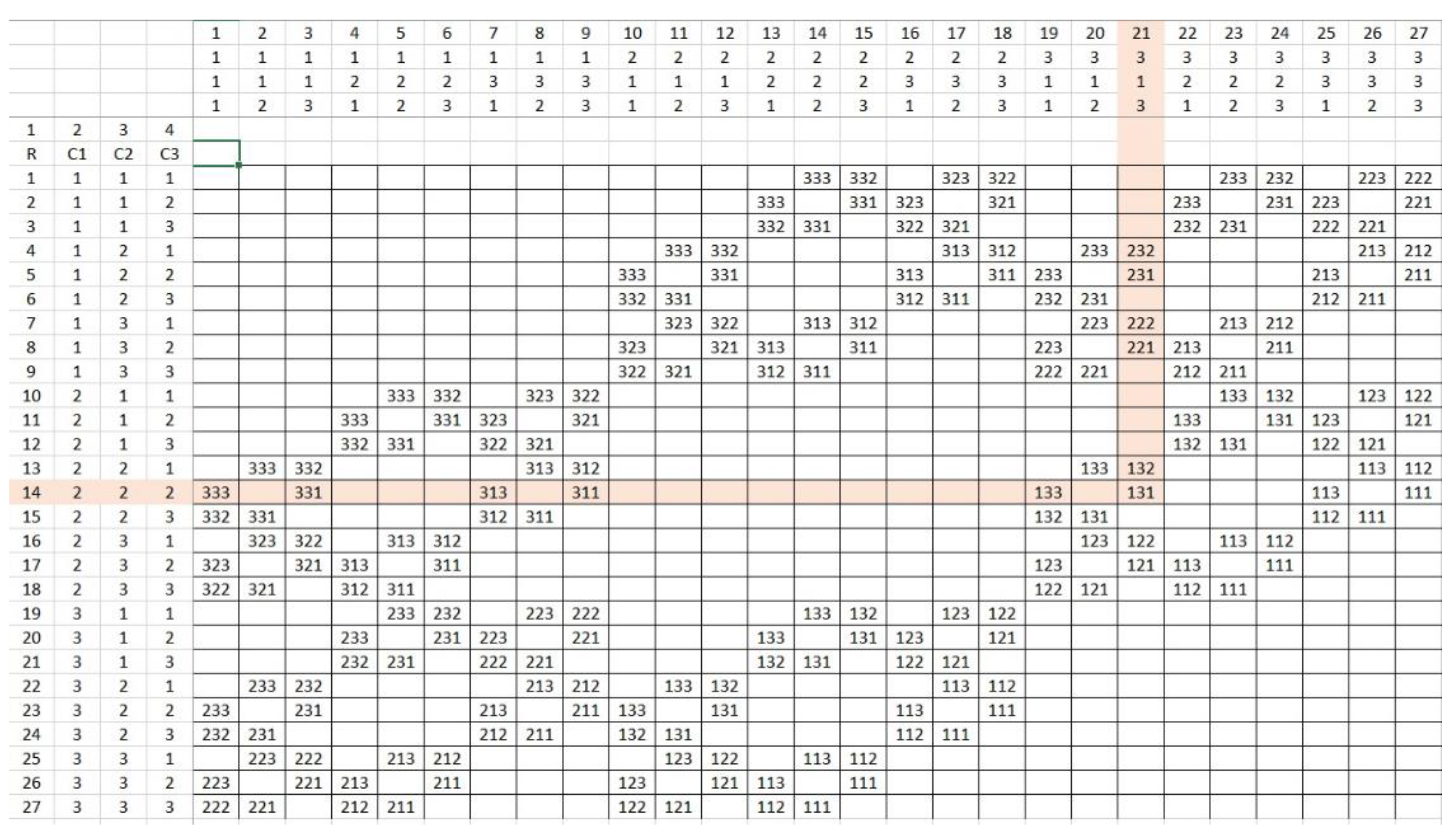
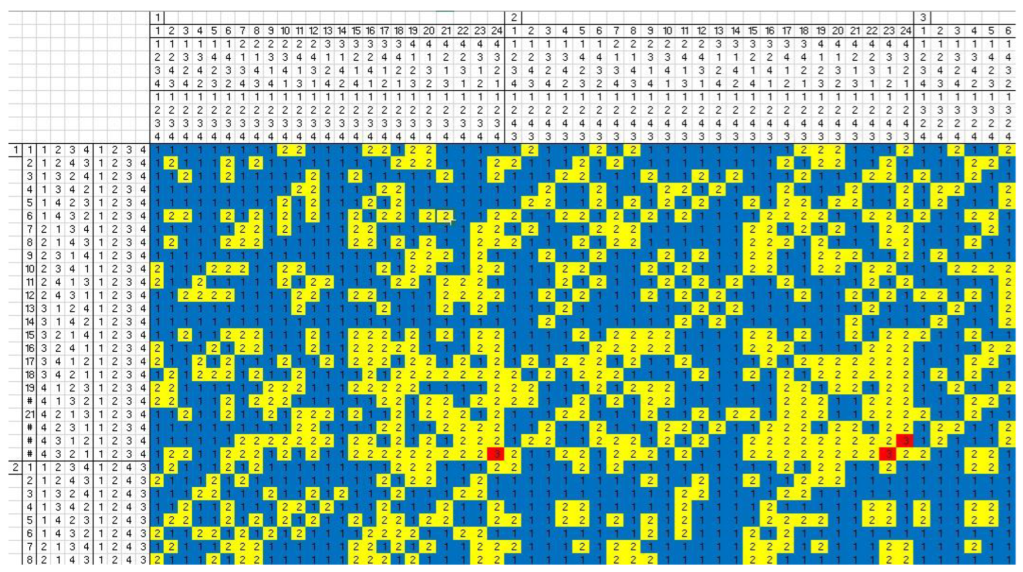
4.1. Magic Square and Conflict Matrix Classification
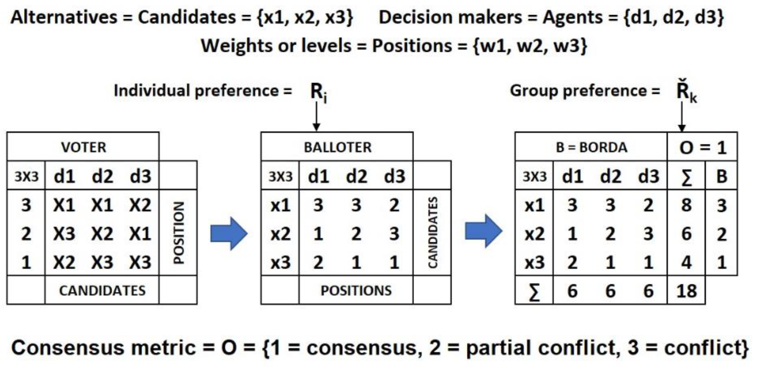
4.2. Definitions for Voting Procedures
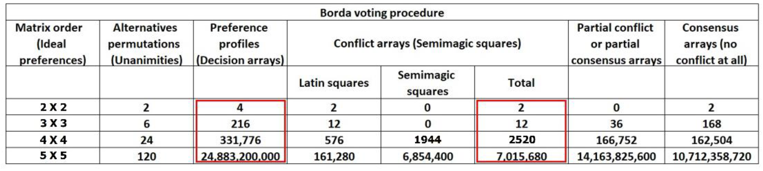
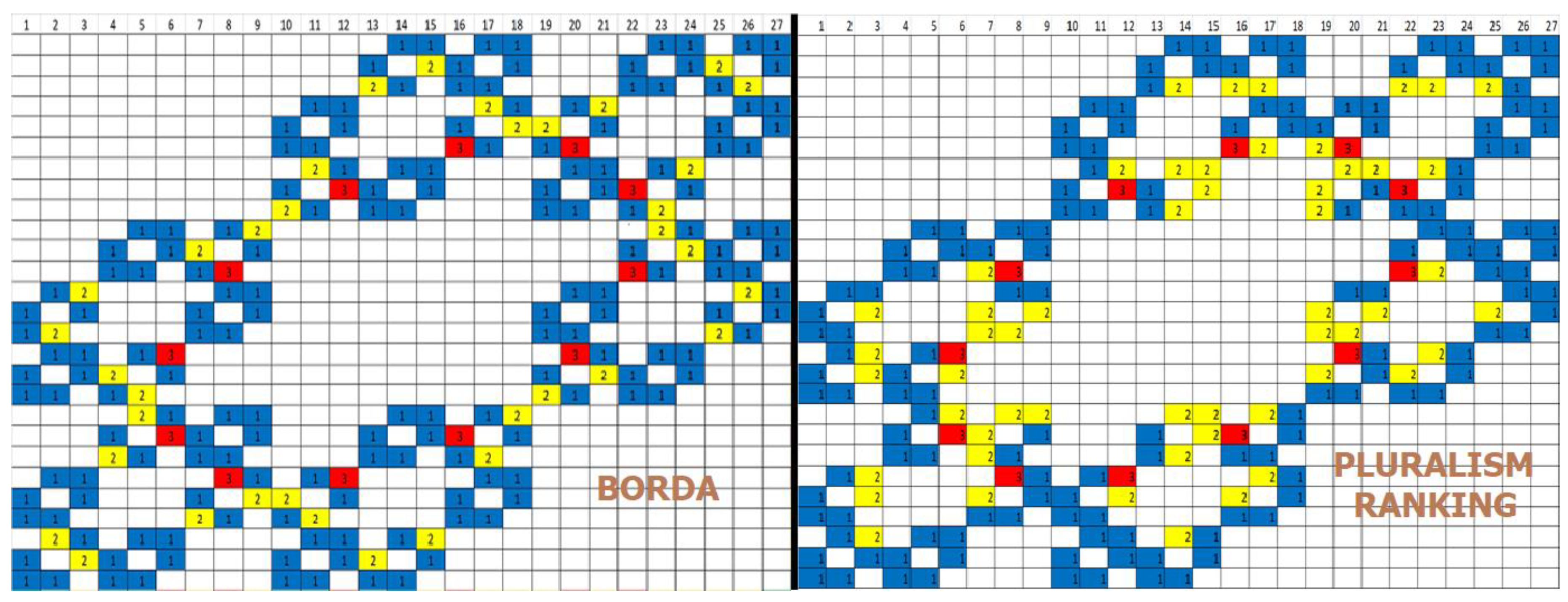
4.3. Borda Voting Procedure
4.4. Stronger Alternative (Candidate) Profile Anatomy Matrix
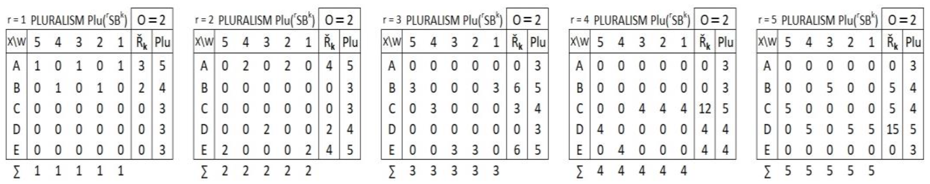
4.5. Pluralism Voting Procedure
4.6. Pluralism Ranking Voting Procedure
4.7. Condorcet’s Ranking Voting Procedure
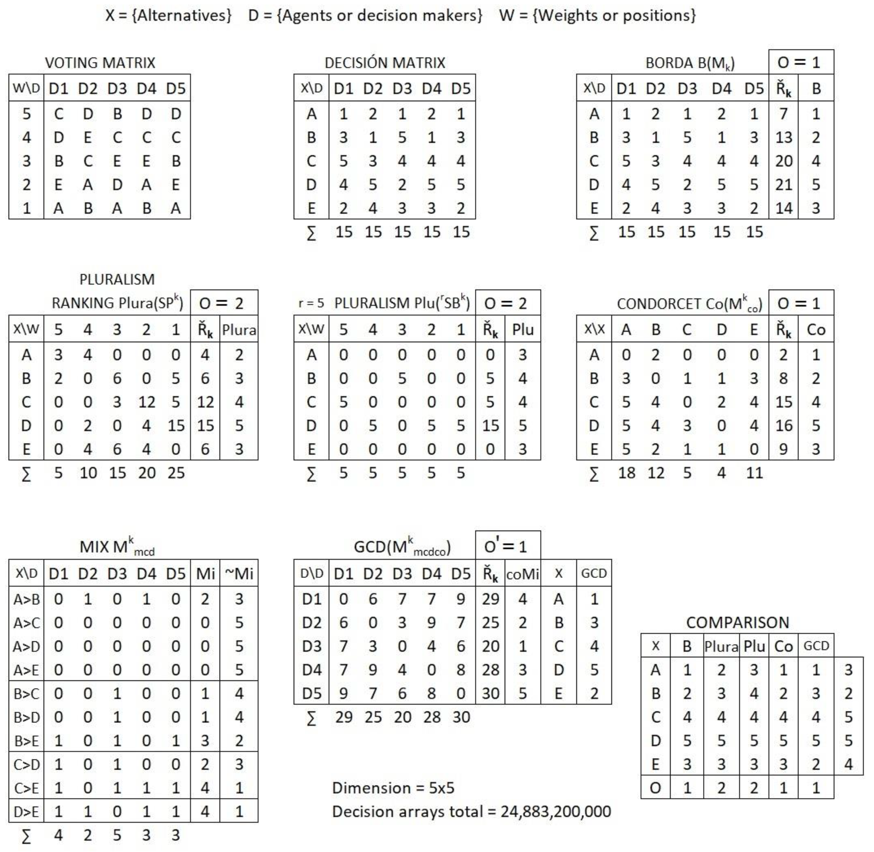
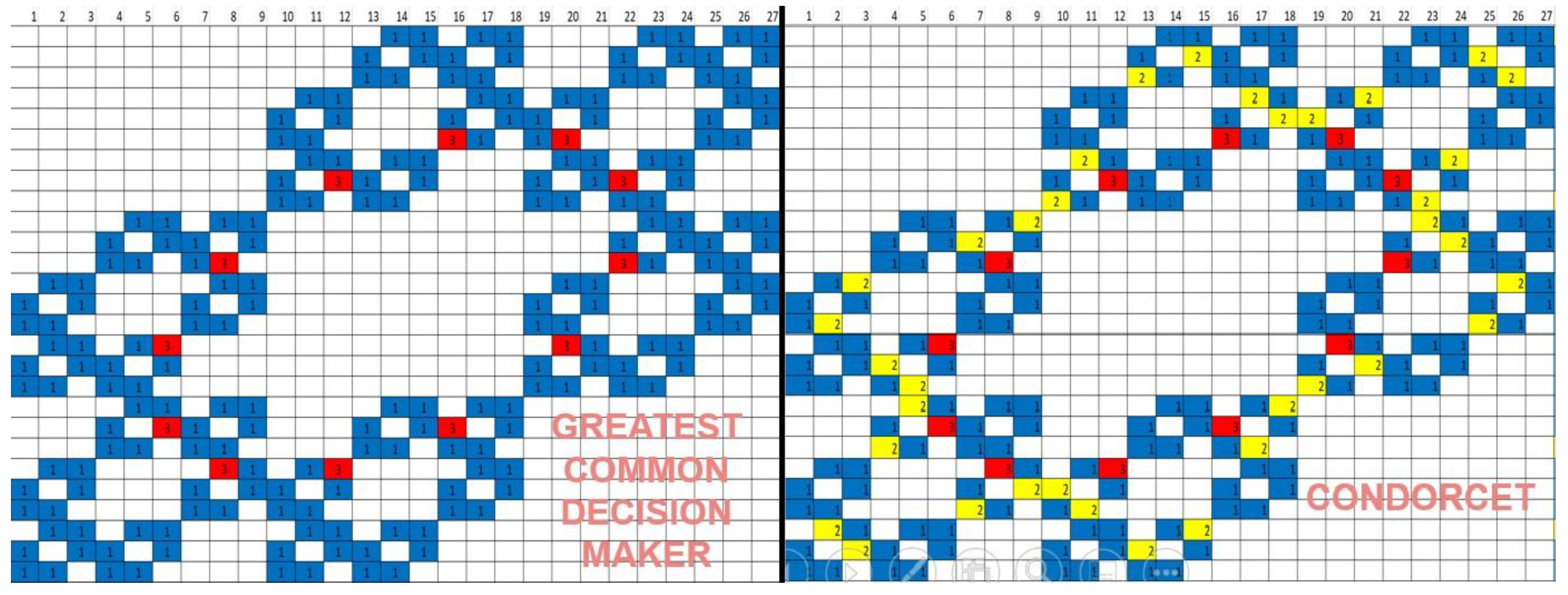
4.8. Greatest Common Decision Maker Ranking Voting Procedure
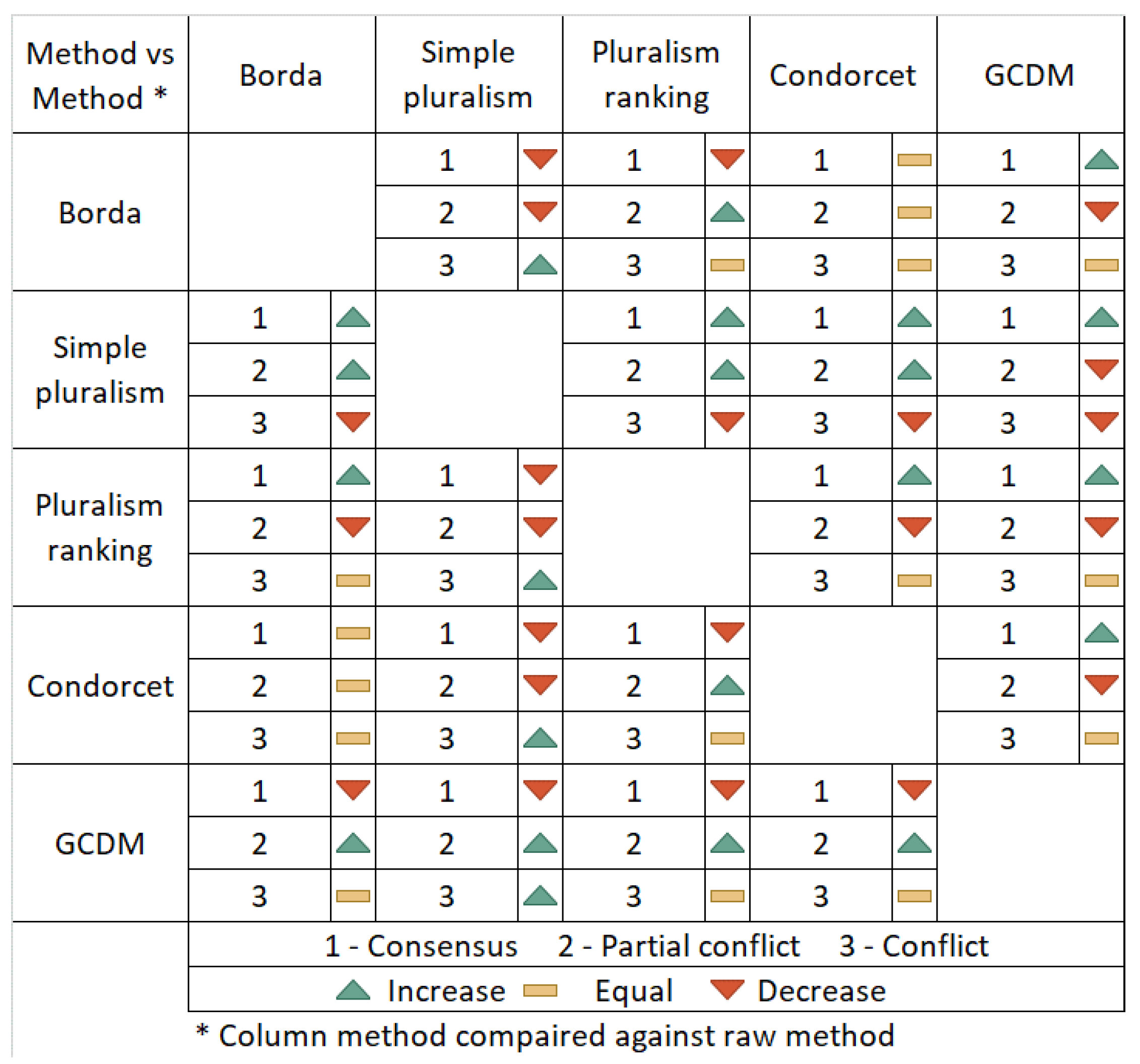
4.9. Examples of Voting Rule Dynamics
5. Frameworks, Tools, and Methods
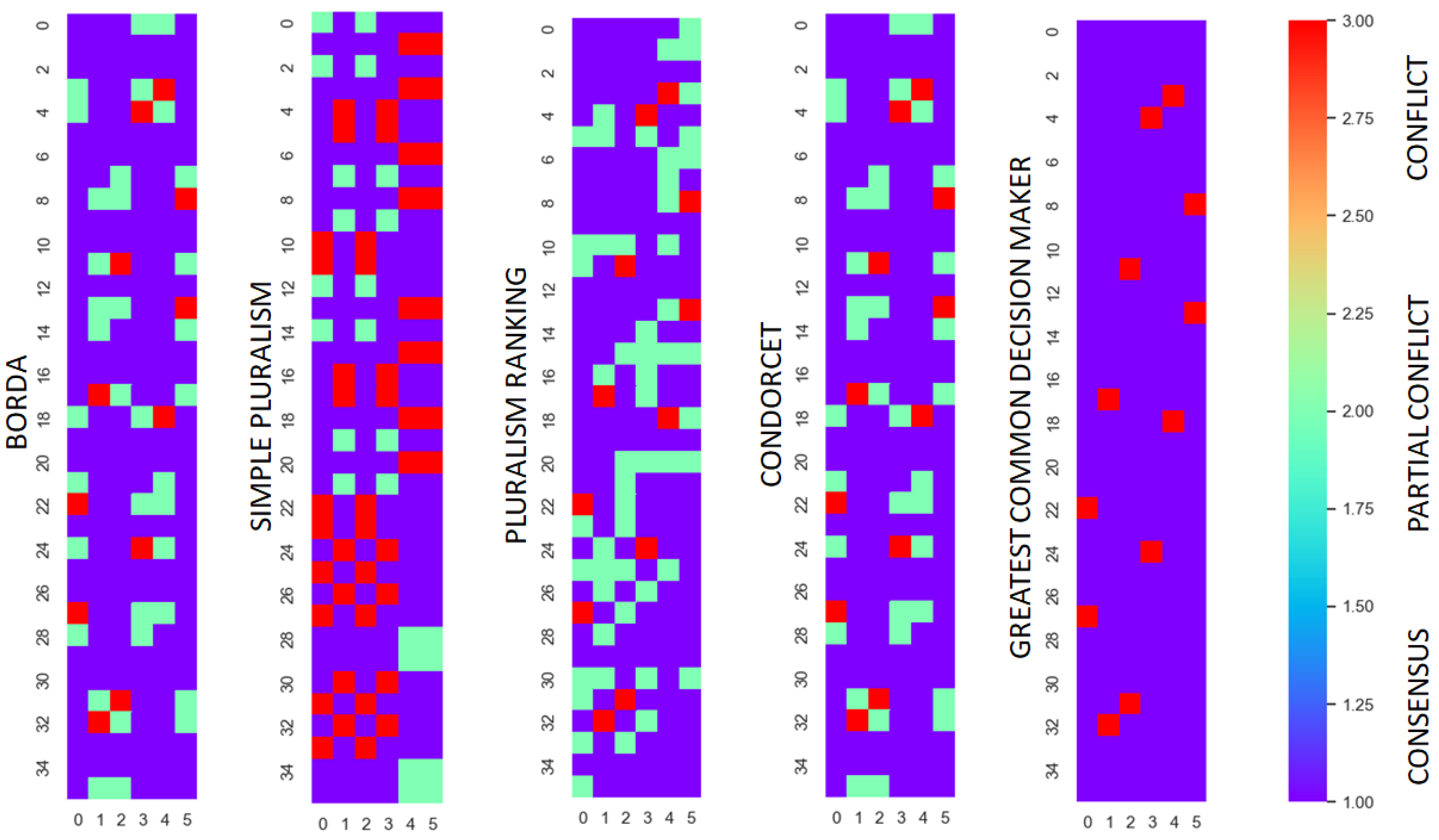
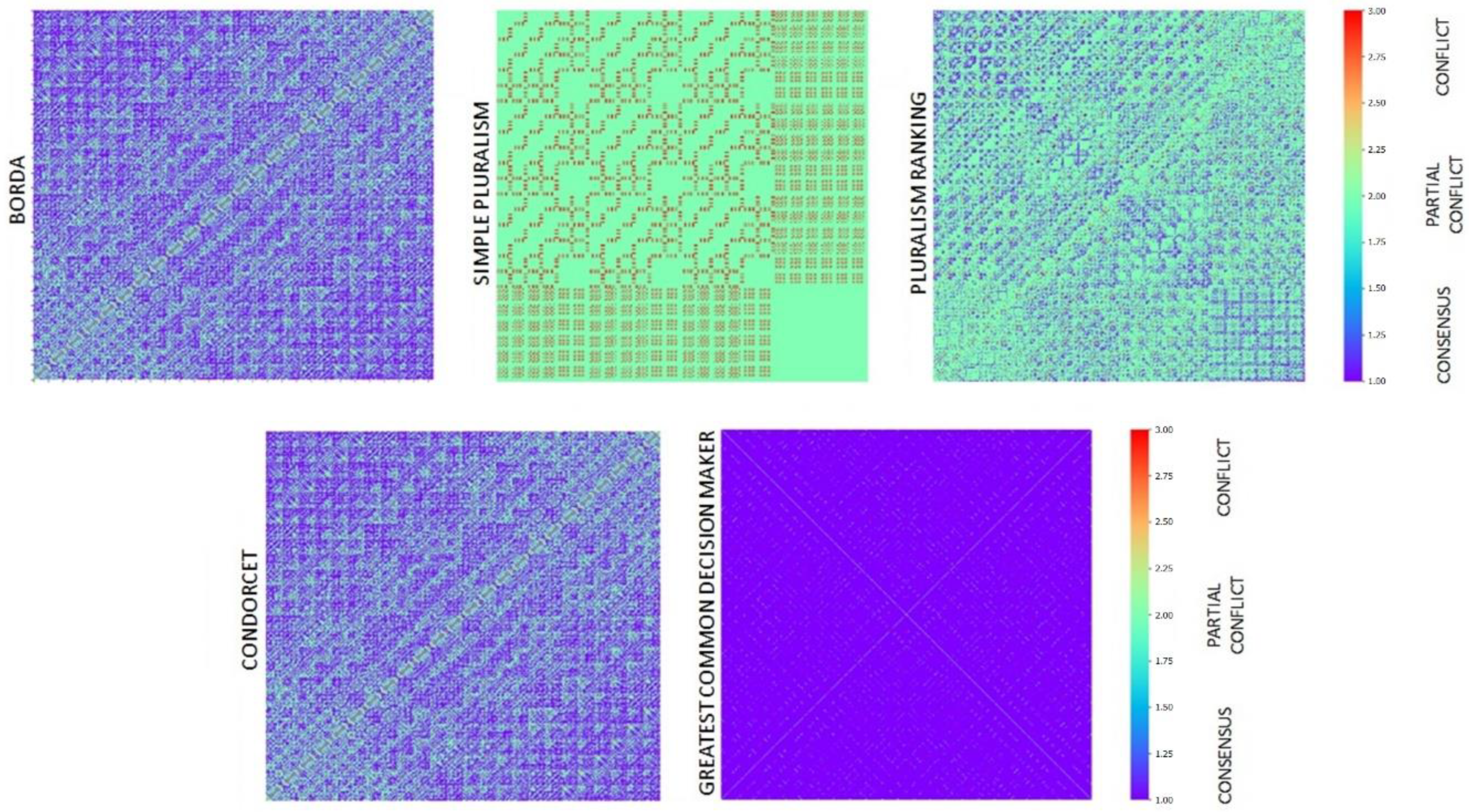
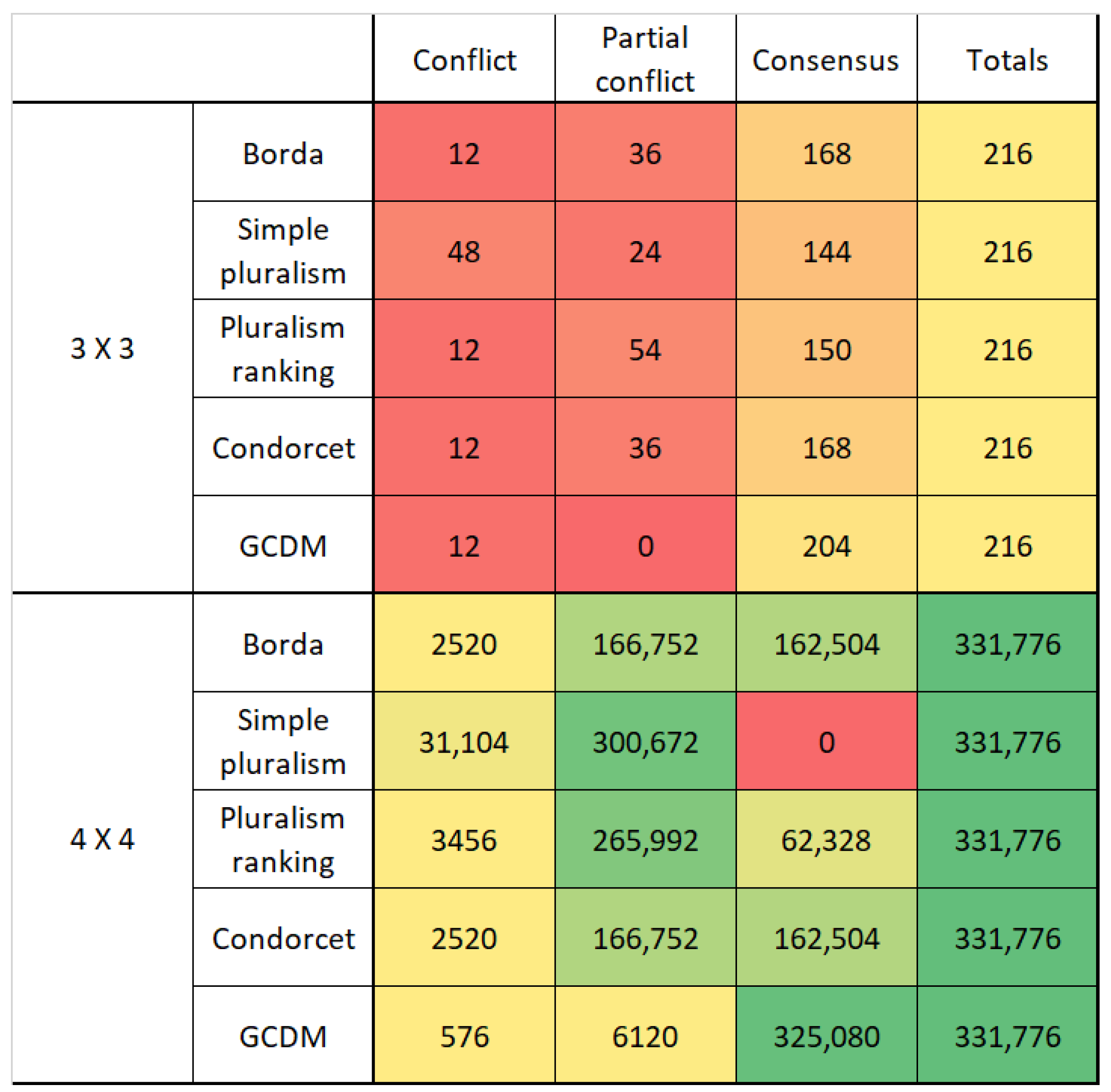
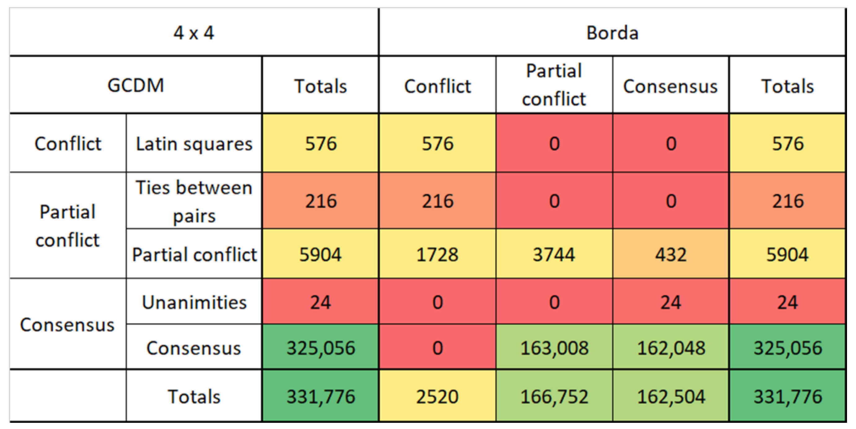
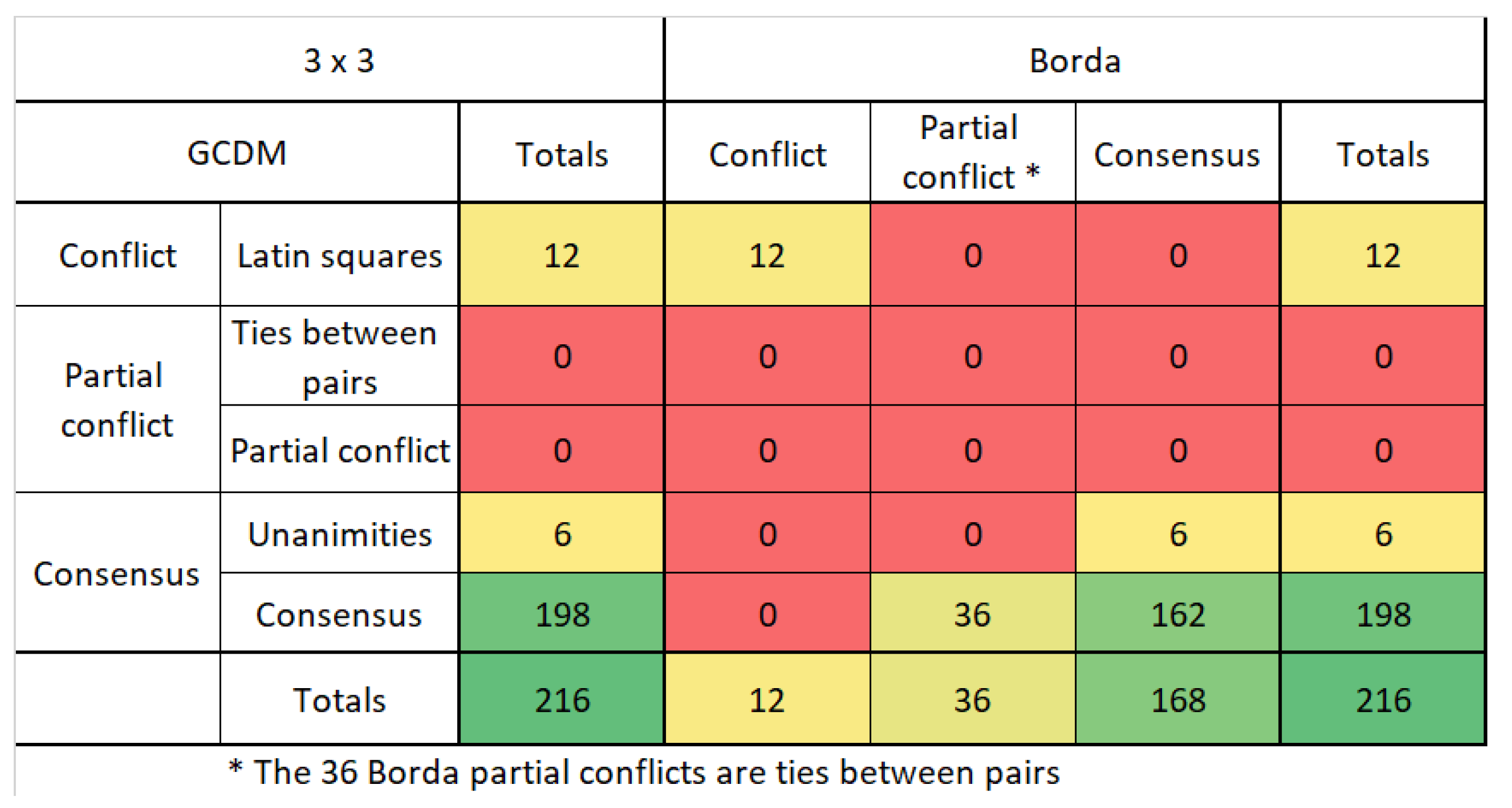
6. Results
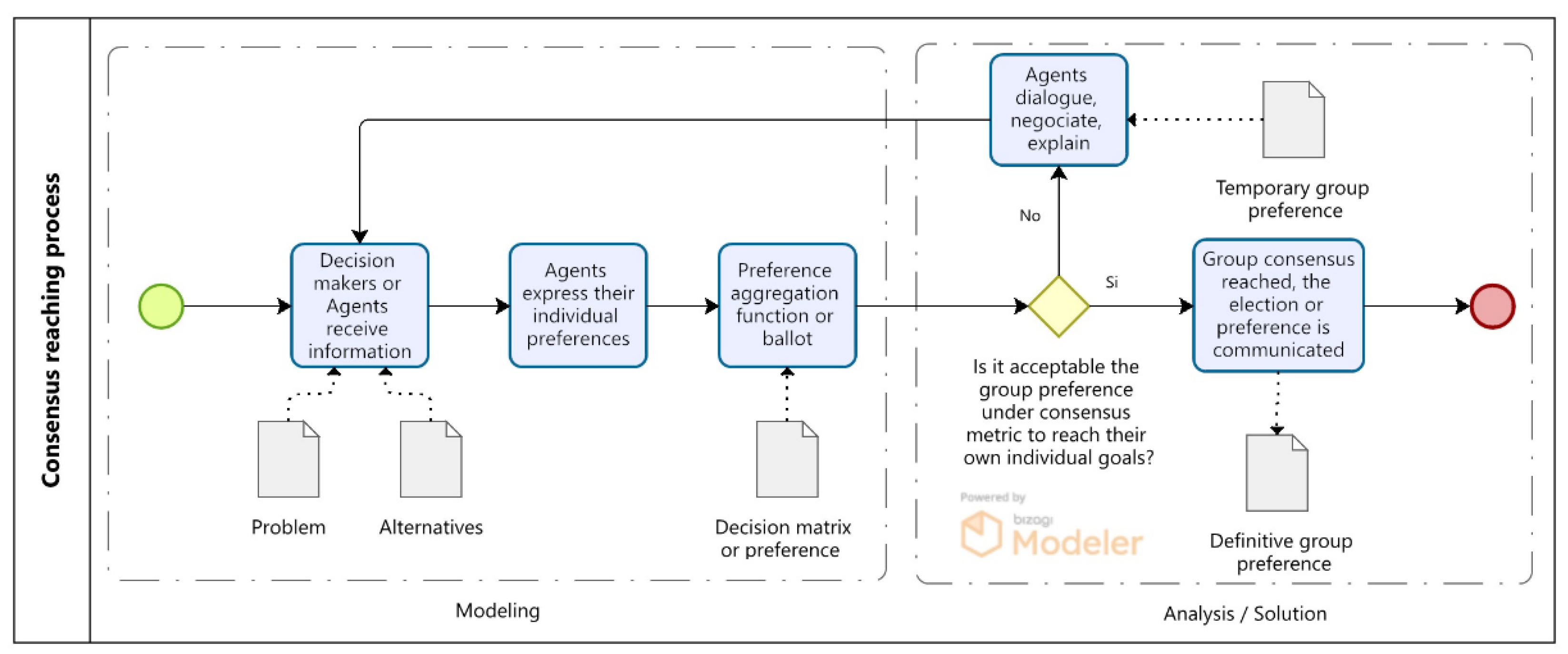
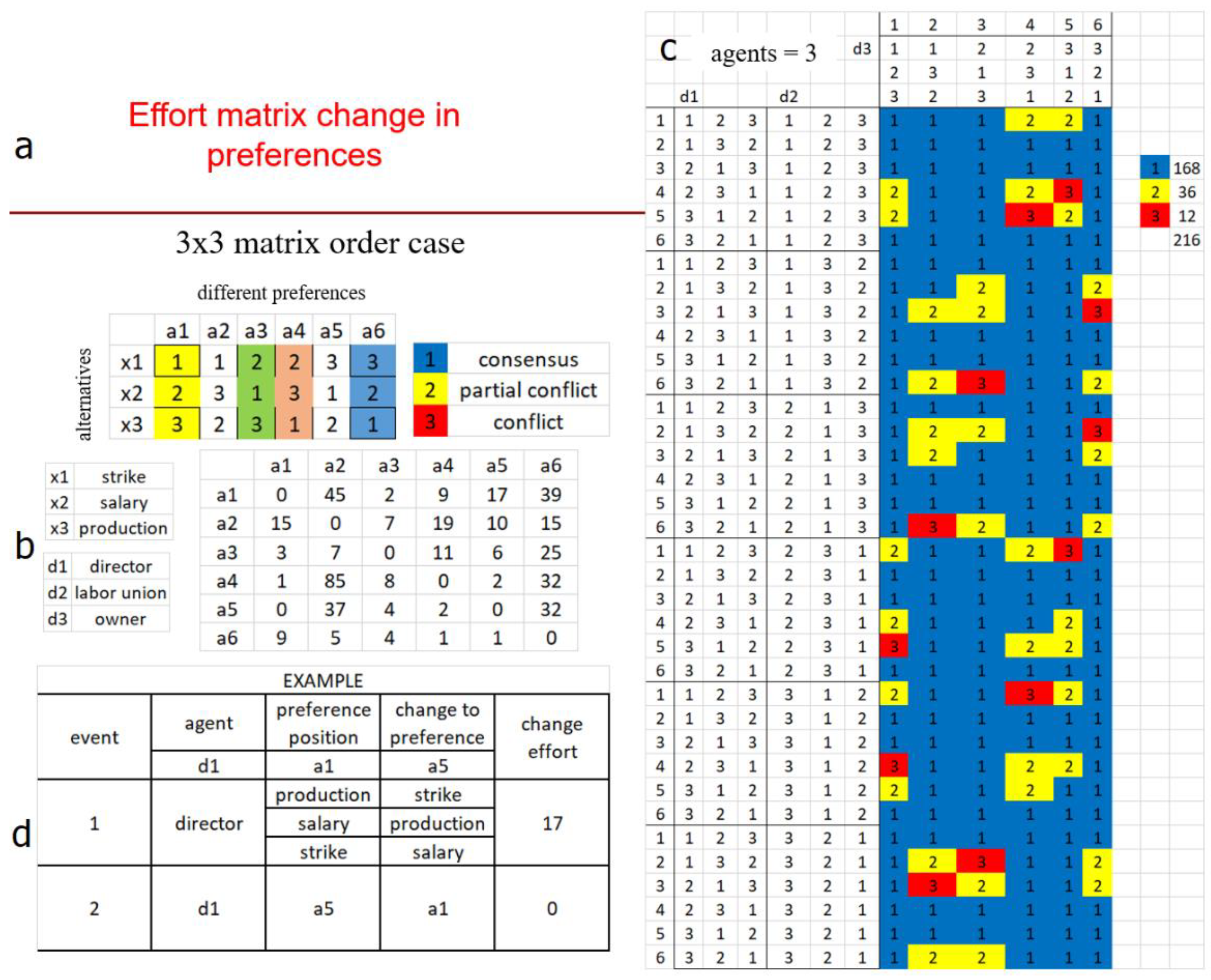
Consensus Reaching Process in the Dynamic Phase, a Cost Decision Visualization
7. Discussion
- The need to organize a large number of decision matrices or preference profiles. In real-life environments, it is not usual to face voting selections among large amounts of objects, but few of them.
- The amount of time needed to organize all possible combinations of objects to be elected from the alternative set. Additionally, performing them naturally to evaluate the strategies for each agent and map conflict was also difficult.
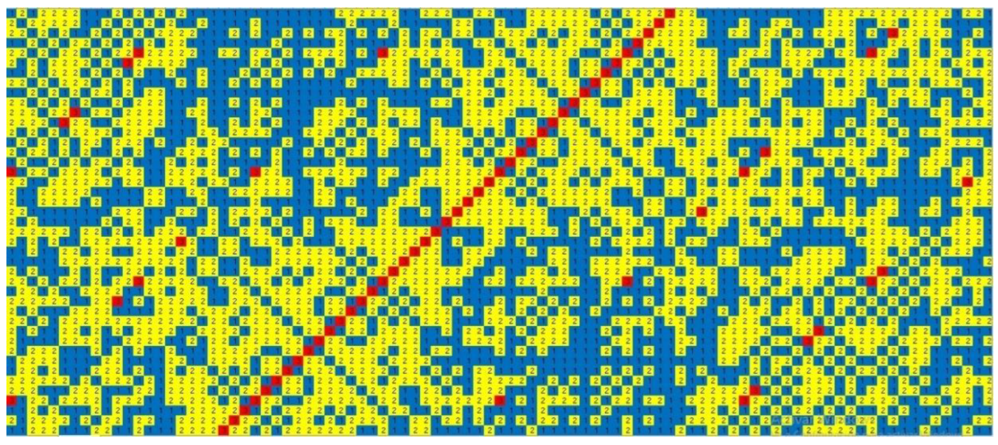
- In the static phase, the aggregation preference procedures played a significant role, while in the dynamic phase the conflict maps did.
- It is necessary to know all the types of conflict matrices to understand what role they play in the process of reaching consensus negotiation [54].
- Our research allowed us to identify that the decision problems under our assumptions have fractal behavior patterns and computational complexity of the NP type [78].
- Higher frequency is better than higher weight.
- Majority is not consensus. Majority is democracy.
- Ordering means decision-making agent election order.
- Weight does not mean a majority.
- Assigning a weight is relative to each person and it is an individual opinion.
- A decision matrix, preference matrix, or conflict matrix is a semi-magic square, ordinary magic square, or a Latin square.
Future Work
8. Conclusions
Author Contributions
Funding
Data Availability Statement
Acknowledgments
Conflicts of Interest
Appendix A. Abbreviations
| CRP | Consensus reaching process |
| GDM | Group decision making |
| (n, n − 1,..., 1) | Ordinal ranking |
| X | Set of alternatives |
| xi | Alternative “i” |
| i | Represents the number of the alternative |
| D | Panel of experts or decision makers |
| di | Decision maker or agent “i” |
| m | Represents the number of the decision maker |
| W | Set of preference weights |
| Wi | Weight assigned to alternative “i” |
| x > y | “x” is preferred to “y” |
| R | A linear order |
| Rj or Pj | An individual preference or linear order associated with decision maker dj |
| Řk | A preference or linear order which is associated as a group preference of the “m” decision makers in the set D |
| M | An array that represent the preference data collected from “m” agents |
| |L(X)| | Cardinality of set L(X) |
| #A | Cardinality of a set A |
| RjT | Transposed matrix of Rj |
| Mk | Decision matrix (or group choice profile) which represents the individual preference arrangement of a set of agents D |
| rSBk | Weight submatrix profile |
| SPk | Stronger alternative (candidate) profile matrix |
| Mkco | Condorcet matrix |
| Mkcod | Condorcet decision maker’s matrix |
| Mkmcd | Mix matrix |
| Mkmcdco | Condorcet mix matrix |
| O(v) | Conflict metric or function that calculates the degree of conflict–consensus |
| O’(v) | Conflict metric or function that calculates the degree of conflict-consensus for the Greatest Common Decision Maker |
| v | Vector of weights or Řk |
| B | Borda aggregation function |
| Plu | Pluralism aggregation function |
| Plura | Pluralism ranking aggregation function |
| SUBr | Weight submatrix profile function |
| SAPA | Stronger alternative profile function |
| GCD | Greatest Common Decision Maker aggregation function |
| Co | Condorcet aggregation function |
| CoD | Condorcet decision maker’s aggregation function |
Appendix B. Demonstration that n!m Is the Total Cardinality Number of the Set of Decision Matrices
- Definition Řk = {w1k, w2k, …, wnk} represents one of the aggregation group preferences of different matrices of dimension “n × m”, where “m” is the number of decision makers and “n” is the number of alternatives. In other words, one group preference Řk is associated one-to-one with a decision matrix.
- From the definition, the set X has “n” alternatives; therefore, n! different orders or permutations of this set exist based on mathematical combinatory. Each permutation is associated one-to-one with a individual preference.
- By definition, if we build a decision matrix M, it has to be a combination of “m” decision makers in this way M = [P1, P2, …, Pm].
- Then, the total permutations allowing repetitions necessary to build the complete set of decision matrices is the multiplication of the “m” decision maker total preferences where each decision maker has, in turn, n! alternatives to select.
- Therefore, the total cardinality number of the set of decision matrices is n!m based on mathematical combinatory QED.
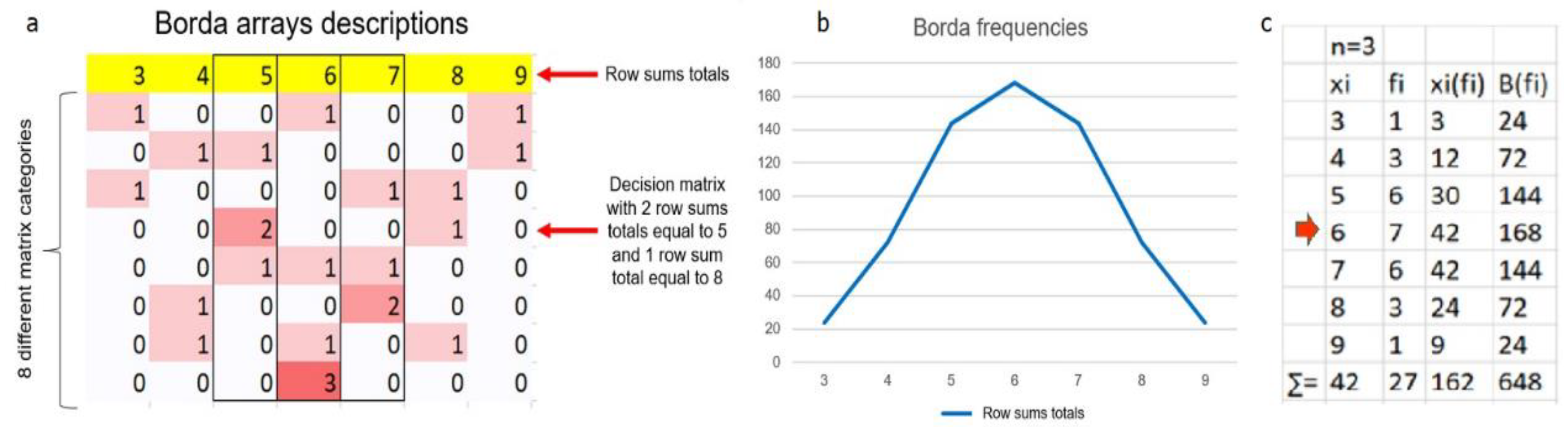
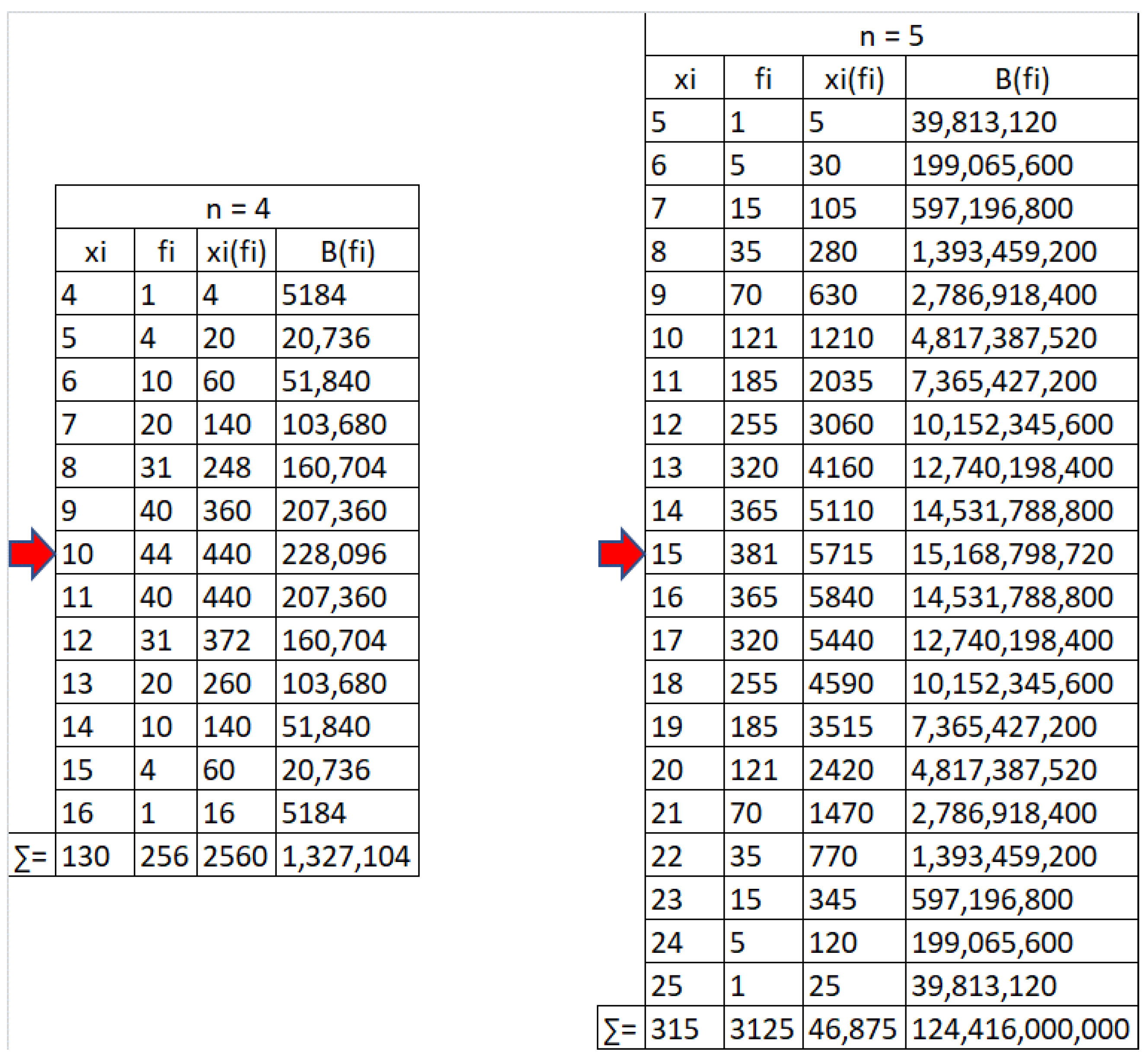
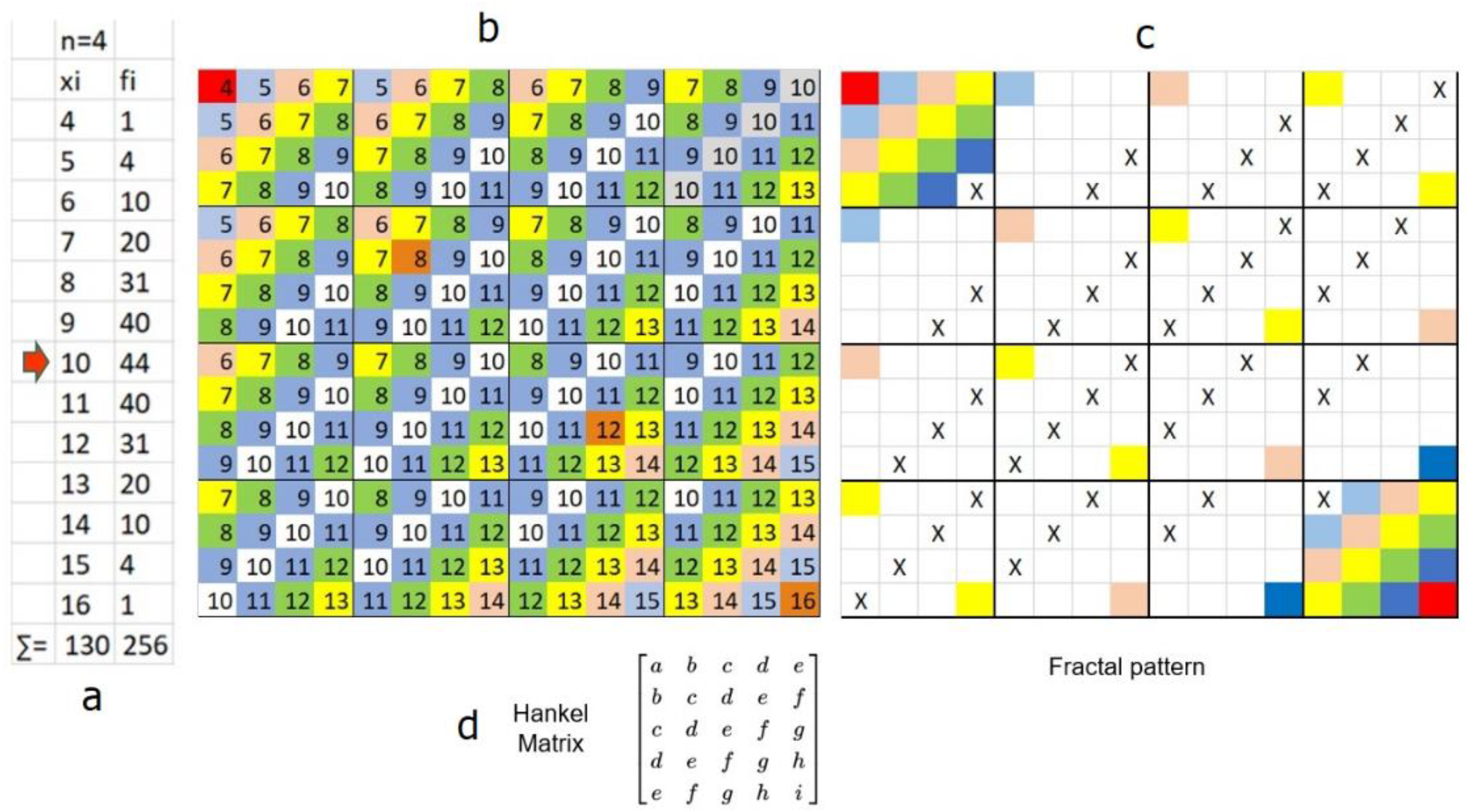
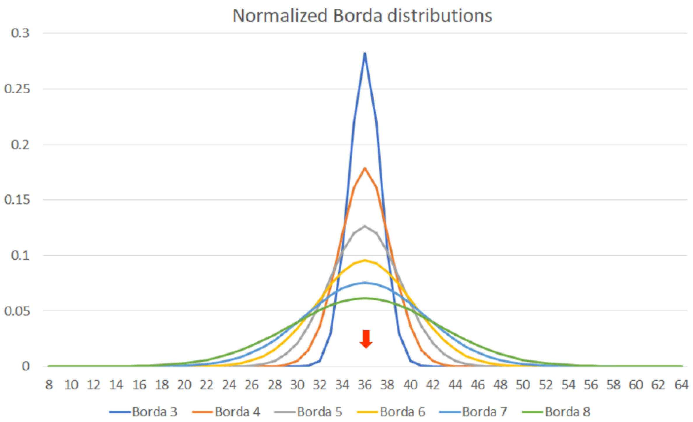
Appendix C. Borda Frequency Tables and Borda Distribution Function


Appendix D. Borda Distribution Function Algorithm
References
- Solución de Conflictos. 2017. Available online: https://www.significados.com/solucion-de-conflictos/ (accessed on 22 June 2019).
- Xu, H.; Hipel, K.W.; Kilgour, D.M.; Fang, L. Conflict Resolution Using the Graph Model: Strategic Interactions in Competition and Cooperation; Studies in Systems, Decision and Control; Springer International Publishing AG: Cham, Switzerland, 2018; Volume 153. [Google Scholar]
- García-del-Valle, P.; Hernández-Martínez, E.G.; Fernández-Anaya, G. A Methodology for the Analysis of Cooperation and Conflict, in the Consensus-Negotiation; XXIII SIMMAC: San José, Costa Rica, 2022. [Google Scholar]
- Heckerman, D.E.; Horvitz, E.J.; Nathwani, B.N. Toward Normative Expert Systems: Part I The Pathfinder Project. Methods Inf. Med. 1992, 31, 90–105. [Google Scholar] [CrossRef] [PubMed]
- Aliev, R.A.; Pedrycz, W.; Kreinovich, V.; Huseynov, O.H. The General Theory of Decisions. Inf. Sci. 2016, 327, 125–148. [Google Scholar] [CrossRef]
- Kreps, D.M. Notes on the Theory of Choice; Underground Classics in Economics; Westwiew Press, Inc.: Boulder, CO, USA, 1988. [Google Scholar]
- Doyle, J.; Thomason, R.H. Background to qualitative decision theory. AI Mag. 1999, 20, 55. [Google Scholar]
- Ganesh, S.; Samik, B.; Vasant, H. Representing and Reasoning with Qualitative Preferences for Compositional Systems. J. Artif. Intell. Res. 2011, 42, 211–274. [Google Scholar]
- Novaro, A.; Longin, D.; Grandi, U.; Lorini, E. Individual goals to collective decisions-extended abstract. In Proceedings of the 17th International Conference on Autonomous Agents and Multiagent Systems (AAMAS 2018), Stockholm, Sweden, 10–15 July 2018. [Google Scholar]
- Novaro, A.; Grandi, U.; Longin, D.; Lorini, E. From Individual Goals to Collective Decision. In Proceedings of the 17th International Conference on Autonomous Agents and Multiagent Systems (AAMAS 2018), Stockholm, Sweden, 10–15 July 2018. [Google Scholar]
- Boutilier, C.; Brafman, R.I.; Domshlak, C.; Hoos, H.H.; Poole, D. CP-net: A tool for representing and reasoning with Conditional Ceteris Paribus Preference Statements. J. Artif. Intell. Res. 2004, 21, 135–191. [Google Scholar] [CrossRef]
- Mella, P. The Combinatory Systems Theory, Understanding, Modeling, and Simulating Collective Phenomena; Contemporary Systems Thinking; Springer: Berlin/Heidelberg, Germany, 2017. [Google Scholar]
- Daniëls, T.R. Social Choice and the Logic of Simple Games. J. Log. Comput. 2011, 21, 883–906. [Google Scholar] [CrossRef]
- Castro, J.F.T.D.; Costa, H.G.; Méxas, M.P.; Lima, C.B.D.C.; Ribeiro, W.R. The influence of factors on project management: A qualitative approach. Production 2021, 31, e20200112. [Google Scholar] [CrossRef]
- Matini, C.; Sprenger, J. Opinion Aggregation and Individual Expertise. Academy of Finland Centre of Excellence in the Philosophy of the Social Sciences, Department of Political and Economic Studies. 2015. Available online: http://hdl.handle.net/2318/1662568 (accessed on 1 October 2022).
- Xia, L. The Smoothed Possibility of Social Choice. Adv. Neural Inf. Process. Syst. 2020, 33, 11044–11055. [Google Scholar]
- Tang, P.; Lin, F. Computer-aided proofs of Arrow’s and other impossibility theorems. Artif. Intell. 2009, 173, 1041–1053. [Google Scholar] [CrossRef] [Green Version]
- Palomares, I.; Martinez, L. A semisupervised multiagent system model to support consensus-reaching process. IEEE Trans. Fuzzy Syst. 2013, 22, 762–777. [Google Scholar] [CrossRef]
- Zhang, H.; Dong, Y.; Chiclana, F.; Yu, S. Consensus efficiency in group decision making: A comprehensive comparative study and its optimal design. Eur. J. Oper. Res. 2019, 275, 580–598. [Google Scholar] [CrossRef]
- Mata, F.; Sánchez, P.; Palomares, I.; Quesada, J.F.; Martínez, L. COMAS: A consensus multi-agent based system. In Proceedings of the 2010 10th International Conference on Intelligent Systems Design and Applications, Cairo, Egypt, 29 November 2010–1 December 2010. [Google Scholar]
- Cook, W.D.; Seiford, L.M. On the Borda-Kendall consensus method for priority ranking problems. Manag. Sci. 1982, 28, 621–637. [Google Scholar] [CrossRef]
- Lichbach, M.I. Is Rational Choice Theory All of Social Science? The University of Michigan Press: Ann Arbor, MI, USA, 2003; ISBN 978-0-472-06819-7. [Google Scholar]
- Brachman, R.J.; Rossi, F.; Stone, P. Learning and Decision-Making from Rank Data. Synth. Lect. Artif. Intell. Mach. Learn. 2019, 13, 1–159. [Google Scholar]
- Silva, G. La Teoría del Conflicto. Un marco teórico necesario. Prolegómenos. Derechos y Valores; Universidad Militar Nueva Granada: Bogotá, Colombia, 2008; Volume XI, pp. 29–43. [Google Scholar]
- Patterson, K.; Grenny, J.; McMillan, R.; Switzler, A. Crucial Conversations: Tools for Talking When Stakes Are High; McGraw-Hill Education: New York, NY, USA, 2011. [Google Scholar]
- Internet Encyclopedia of Philosophy. Available online: https://iep.utm.edu/hobmeth/ (accessed on 22 June 2022).
- Cardona, P. Political Power, Contract and Civil Society: From Hobbes to Locke; Revista Facultad de Derecho y Ciencias Políticas: Medellín, Colombia, 2008; Volume 38, pp. 123–154. [Google Scholar]
- Gonnet, J. Orden social y conflicto en la teoría de los sistemas de Niklas Luhmann. Cinta Moebio 2018, 61, 110–122. [Google Scholar] [CrossRef]
- Emergence. Available online: https://en.wikipedia.org/wiki/Emergence (accessed on 14 May 2020).
- Johnson, S. Emergence: The Connected Lives of Ants, Brains, Cities and Software; Gardners Books: Eastbourne, UK, 2002. [Google Scholar]
- Delic, A.; Neidhardt, J.; Nguyen, T.N.; Ricci, F. Research Methods for Group Recommender Systems. In Proceedings of the 10th ACM Conference on Recommender Systems (RecSys), Boston, MA, USA, 15 September 2016. [Google Scholar]
- Werbin-Ofir, H.; Dery, L.; Shmueli, E. Beyond Majority: Label Ranking Ensembles based on Voting Rules. Expert Syst. Appl. 2019, 136, 50–61. [Google Scholar] [CrossRef]
- Horio, B.M.; Shedd, J.R. Agent-based exploration of the political influence of community leader on population opinion dynamics. In Proceedings of the 2016 Winter Simulation Conference (WSC), Washington, DC, USA, 11–14 December 2016. [Google Scholar]
- Rosanisah, W.; Mohd, W.; Abdullah, L. Aggregation Methods in Group Decision Making: A Decade Survey. Informatica 2017, 41, 71–86. [Google Scholar]
- Gleb, B.; Tomasa, C.; Simon, J. Consensus measures constructed aggregation functions and fuzzy implications. Knowl. -Based Syst. 2014, 55, 1–8. [Google Scholar]
- Zhen, Z.; Zhuolin, L. Personalized Individual Semantics-Based Consistency Control and Consensus Reaching in Linguistic Group Decision Making. IEEE Trans. Syst. Man Cybern. Syst. 2022, 52, 5623–5635. [Google Scholar]
- Li, Z.; Zhang, Z.; Yu, W. Consensus reaching with consistency control in group decision making with incomplete hesitant fuzzy linguistic preference relations. Comput. Ind. Eng. 2022, 170, 108311. [Google Scholar] [CrossRef]
- Gai, T.; Cao, M.; Chiclana, F.; Zhang, Z.; Dong, Y.; Herrera-Viedma, E.; Wu, J. Consensus-trust Driven Bidirectional Feedback Mechanism for Improving Consensus in Social Network Large-group Decision Making. Group Decis. Negotation 2022. [Google Scholar] [CrossRef]
- Wan, S.P.; Yan, J.; Dong, J.Y. Personalized individual semantics based consensus reaching process for large-scale group decision making with probabilistic linguistic preference relations and application to COVID-19 surveillance. Expert Syst. Appl. 2022, 191, 116328. [Google Scholar] [CrossRef]
- Xu, G.L.; Wan, S.P.; Wang, F.; Dong, J.Y.; Zeng, Y.F. Mathematical programming methods for consistency and consensus in group decision making with intuitionistic fuzzy preference relations. Knowl. -Based Syst. 2016, 98, 30–43. [Google Scholar] [CrossRef]
- Wan, S.; Wang, F.; Dong, J. A group decision-making method considering both the group consensus and multiplicative consistency of interval-valued intuitionistic fuzzy preference relations. Inf. Sci. 2018, 466, 109–128. [Google Scholar] [CrossRef]
- Types of Voting System. 2017. Available online: https://www.electoral-reform.org.uk/voting-systems/types-of-voting-system/ (accessed on 26 April 2021).
- Kacprzyk, J.; Merigó, J.M.; Nurmi, H.; Zadorzny, S. Multi-agent systems and voting: How similar are voting procedures. In Communications in Computer and Information Science Book; Springer: Cham, Switzerland, 2020; Volume 1237. [Google Scholar]
- Chevaleyre, Y.; Endriss, U.; Lang, J.; Maudet, N. A short introduction to computational social choice. In International Conference on Current Trends in Theory and Practice of Computer Science; Springer: Berlin/Heidelberg, Germany, 2008. [Google Scholar]
- El-Helaly, S. The Mathematics of Voting and Apportionment an Introduction; Compact Textbooks in Mathematics; Birkhäuser: Basel, Switzerland, 2019. [Google Scholar]
- McIntee, T.J. Geometric Ways of Understanding Voting Problems; University of California: Irvine, CA, USA, 2015. [Google Scholar]
- Ignacio, Y.T. La Geometría de Borda. Bachelor’s Thesis, Universidad Abierta Interamericana, Buenos Aires, Argentina, April 2014. [Google Scholar]
- Saari, D.G. Geometry of Voting; Springer: Berlin/Heidelberg, Germany, 1994. [Google Scholar]
- Antoniou, E.; Chin, B.; Felt, A.J.; Giraldo, J.H.; Kwon, M.; Offenholley, K.; Ul-haq, I.; Vallin, R.W. Voting Systems; William Paterson University of New Jersey: Wayne, NJ, USA, 2011; Available online: http://archive.dimacs.rutgers.edu/Publications/Modules/Module10-4/dimacs10-4.pdf (accessed on 1 October 2022).
- Kuhlman, C.; Rundensteiner, E. Rank Aggregation Algorithms for Fair Consensus. Proc. VLDB Endow. 2020, 13, 2706–2719. [Google Scholar] [CrossRef]
- Fasth, T.; Larsson, A.; Ekenberg, L.; Danielson, M. Measuring Conflicts Using Cardinal Ranking: An Application to Decision Analytic Conflict Evaluations. Adv. Oper. Res. 2018, 2018, 8290434. [Google Scholar] [CrossRef]
- Tuba Ahmed, M.; Muzaher Hussain, M.; Keerthi Chennam, K. Designing a Consensus Ranking Algorithm for same domain entities. In Proceedings of the 2017 2nd International Conference on Communication and Electronics Systems (ICCES), Coimbatore, India, 19–20 October 2017. [Google Scholar]
- Li, Y.; Ji, Y.; Qu, S. Consensus Building for Uncertain Large-Scale Group Decision-Making Based on the Clustering Algorithm and Robust Discrete Optimization. Group Decis. Negot. 2022, 31, 453–489. [Google Scholar] [CrossRef]
- Zlotkin, G.; Rosenschein, J.S. Mechanisms for automated negotiation in state oriented domains. J. Artif. Intell. Res. 1996, 5, 163–238. [Google Scholar] [CrossRef]
- Axelrod, R. The Evolution of Cooperation; Basic Books; A Member of the Perseus Books Group: Cambridge, MA, USA, 1984. [Google Scholar]
- Petcu, A.; Faltings, B.; Parkes, D.C. M-DPOP: Faithful distributed implementation of efficient social choice problems. J. Artif. Intell. Res. 2008, 1–8. Available online: https://www.cs.cmu.edu/~sandholm/cs15-892F15/MDPOP-AAMAS06.pdf (accessed on 1 October 2022).
- Palomares, I.; Killough, R.; Bouters, K.; Liu, W.; Hong, J. A collaborative Multiagent Framework based online Risk-Aware Planning and Decision-Making. In Proceedings of the 2016 IEEE 28th International Conference on Tools with Artificial Intelligence (ICTAI), San Jose, CA, USA, 6–8 November 2016. [Google Scholar]
- Suhat Dolapchiev, M.; Martínez Panero, M. Modernas Variantes de la Regla de Votación de Borda. Bachelor´s Thesis, Universidad de Valladolid, Valladolid, Spain, 2018. [Google Scholar]
- Fernando, T.; Federico, F.; Marcelo, A. Inductive Reasoning in Social Choice Theory. J. Log. Lang. Inf. 2019, 28, 551–575. [Google Scholar]
- Barthélemy, J.P.; Janowitz, M.F. A formal theory of consensus. Soc. Ind. Appl. Math. 1991, 4, 305–322. [Google Scholar] [CrossRef]
- Cuadrado Mágico. Available online: https://www.allmathwords.org/es/m/magicsquare.html (accessed on 25 May 2022).
- Cuadrados Mágicos. Available online: https://ttm.unizar.es/2019-20/TTM2019_CUADRADOS_MGICOS.pdf (accessed on 25 May 2022).
- Cortés, C.I. Propiedades y Aplicaciones de los Cuadrados Latinos. Master’s Thesis, Universidad Autónoma Metropolitana, Ciudad de México, Mexico, 26 October 2011. [Google Scholar]
- Matthias, B.; Moshe, C.; Jessica, C.; Paul, G. The number of magic squares, and hypercubes. Am. Math. Mon. 2003, 110, 707–717. [Google Scholar]
- Magic Square. Available online: http://www.mathematische-basteleien.de/magsquare.htm (accessed on 25 May 2022).
- Sim, K.A.; Wong, K.B. Magic Square and Arrangement of Consecutive Integers That Avoidsk-Term Arithmetic Progressions. Mathematics 2021, 9, 2259. [Google Scholar] [CrossRef]
- Egan, J.; Wanless, I.M. Latin Squares with Restricted Transversals. J. Comb. Des. 2012, 20, 344–361. [Google Scholar] [CrossRef]
- Jacobson, M.T.; Matthews, P. Generating uniformly distributed random Latin squares. J. Comb. Des. 1996, 4, 405–437. [Google Scholar] [CrossRef]
- Mc Kay, B.D.; Wanless, I.M. Most Latin Squares Have Many Subsquares. J. Comb. Theory 1999, 86, 323–347. [Google Scholar] [CrossRef] [Green Version]
- Shao, J.Y. A formula for the number of Latin squares. Discret. Math. 1992, 110, 293–296. [Google Scholar] [CrossRef] [Green Version]
- Magic Square. Available online: https://mathworld.wolfram.com/MagicSquare.html (accessed on 25 May 2022).
- 3×3 Semi Magic Squares. Available online: https://funpaperandpencilgames.blogspot.com/2019/02/3x3-semi-magic-squares.html (accessed on 25 May 2022).
- Grandi, U. Logical Frameworks for Multiagent Aggregation; ESSLLI: Tübingen, Germany, 2014; Available online: https://www.irit.fr/~Umberto.Grandi/teaching/aggregation (accessed on 1 October 2022).
- Palomares, I.; Liu, J.; Xu, Y.; Martinez, L. Modeling expert´s attitudes in group decision making. Soft Comput. 2012, 16, 1755–1766. [Google Scholar] [CrossRef]
- Zhang, H.; Palomares, I.; Dong, Y.; Wang, W. Managing non-cooperative behaviors in consensus-based multiple attribute group decision making: An approach based on social network analysis. Knowl.-Based Syst. J. 2018, 162, 29–45. [Google Scholar] [CrossRef]
- Visser, S.; Thangarajah, J.; Harland, J. Reasoning about preferences in Intelligent Agent Systems. In Proceedings of the Twenty-Second International Joint Conference on Artificial Intelligence, Barcelona Catalonia, Spain, 16–22 July 2011; pp. 426–431. [Google Scholar]
- Nurmi, H. Assessing Borda’s rule and its modifications. In Designing an All-Inclusive Democracy; Springer: Berlin/Heidelberg, Germany, 2007. [Google Scholar]
- Peña, J.M. Finding Consensus Bayesian Network Structures. AI Access Foundation. J. Artif. Intell. Res. 2011, 42, 661–687. [Google Scholar]
- Beliakov, G.; Pradera, A.; Calvo, T. Aggregation Functions: A Guide for Practitioners; Springer: Berlin/Heidelberg, Germany, 2007. [Google Scholar]
- Gamson, W. A theory of coalition formation. Am. Sociol. Assoc. 1961, 26, 373–382. [Google Scholar] [CrossRef]
- Costa, H.G. AHP-de Borda: A hybrid multicriteria ranking method. Braz. J. Oper. Prod. Manag. 2017, 14, 281–287. [Google Scholar] [CrossRef]
- Rico, N.; Vela, C.R.; Pérez-Fernández, R.; Díaz, I. Reducing the Computational Time for the Kemeny Method by Exploiting Condorcet Properties. Mathematics 2021, 9, 1380. [Google Scholar] [CrossRef]
- Terzopoulou, Z.; Endriss, U. The Borda class: An axiomatic study of the Borda rule on top-truncated preferences. J. Math. Econ. 2021, 92, 31–40. [Google Scholar] [CrossRef]
- Smith, S.B. Chance, Strategy and Choice. An Introduction to the Mathematics of Games and Elections; Cambridge Mathematical Textbooks; Cambridge University Press: Cambridge, UK, 2015. [Google Scholar]
- Emerson, P. The original Borda count and partial voting. Soc. Choice Welf. 2013, 40, 353–358. [Google Scholar] [CrossRef]
- Majority Voting System. Available online: https://ballotpedia.org/Majority_voting_system#cite_note-georgetown-1 (accessed on 25 May 2022).
- Russell, N.F. Complexity of Control of Borda Count Elections. Master’s Thesis, Department of Computer Science, Rochester Institute of Technology, Rochester, NY, USA, 9 July 2007. [Google Scholar]
- Plurality System. Available online: https://www.britannica.com/topic/election-political-science/Plurality-and-majority-systems (accessed on 25 May 2022).
- Morimoto, K. Information Use and the Condorcet Jury Theorem. Mathematics 2021, 9, 1098. [Google Scholar] [CrossRef]
- Condorcet Voting. Available online: https://www.equal.vote/condorcet (accessed on 25 May 2022).
- Darós, W.R. La libertad Individual y el contrato social según J. J. Rousseau. Philos. Mag. 2006, 44, 111–112. [Google Scholar]
- Heradio, R.; Fernandez-Amoros, D.; Cerrada, C.; Cobo, M.J. Group Decision-Making Based on Artificial Intelligence: A Bibliometric Analysis. Mathematics 2020, 8, 1566. [Google Scholar] [CrossRef]
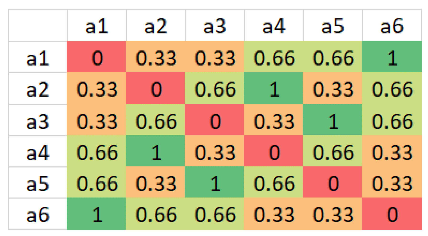
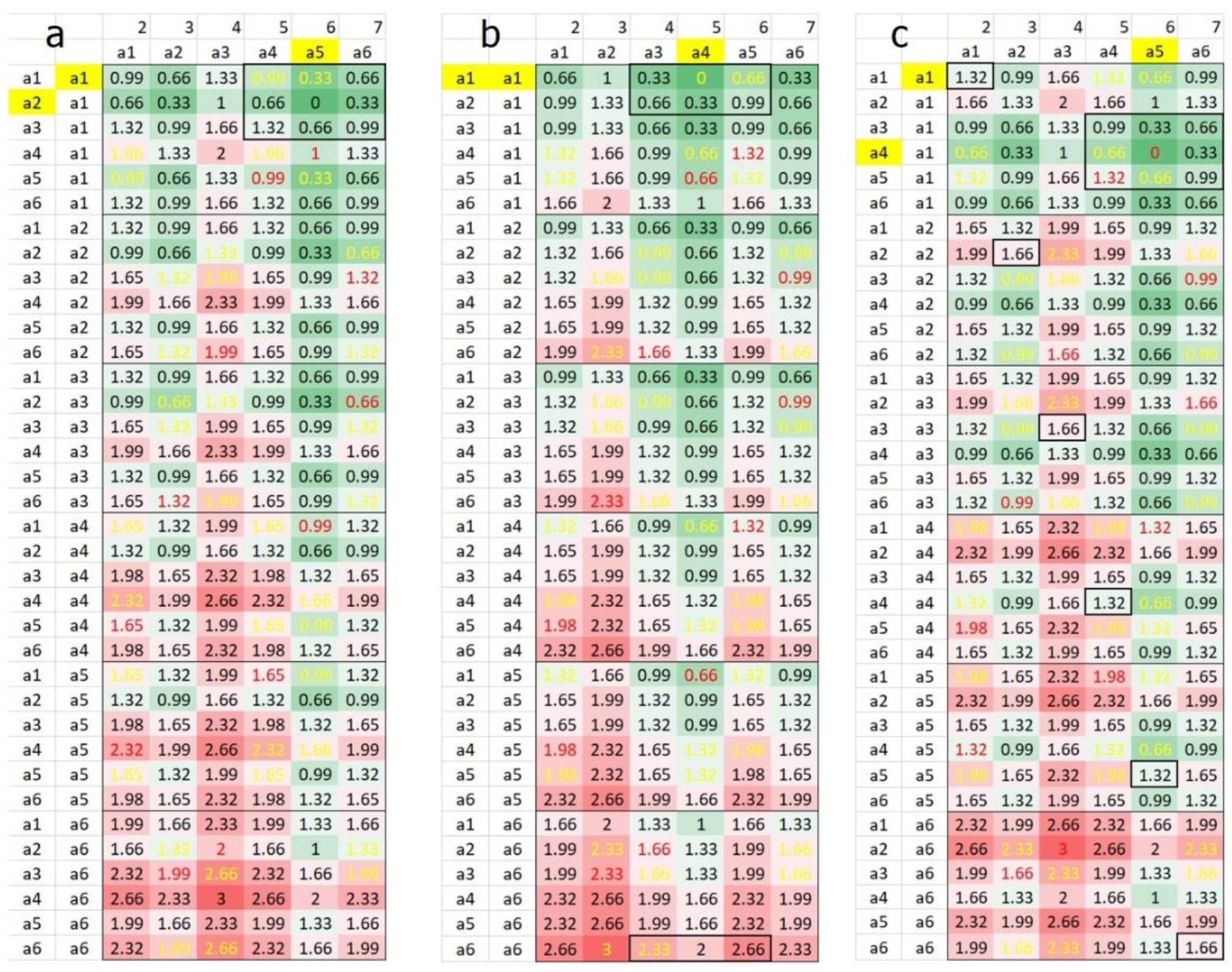
- Heatmap. Available online: https://en.wikipedia.org/wiki/Heat_map (accessed on 25 May 2022).
- Wilkinsona, L.; Friendly, M. The History of the Cluster Heat Map. Am. Stat. 2009, 63, 179–184. [Google Scholar] [CrossRef] [Green Version]
- Hou, F.; Triantaphyllou, E. An iterative approach for achieving consensus when ranking a finite set of alternatives by a group of experts. Eur. J. Oper. Res. 2019, 275, 570–579. [Google Scholar] [CrossRef]
- Yee, K.-P. Voting Simulation Visualizations. 2005. Available online: http://zesty.ca/voting/sim/ (accessed on 6 May 2022).
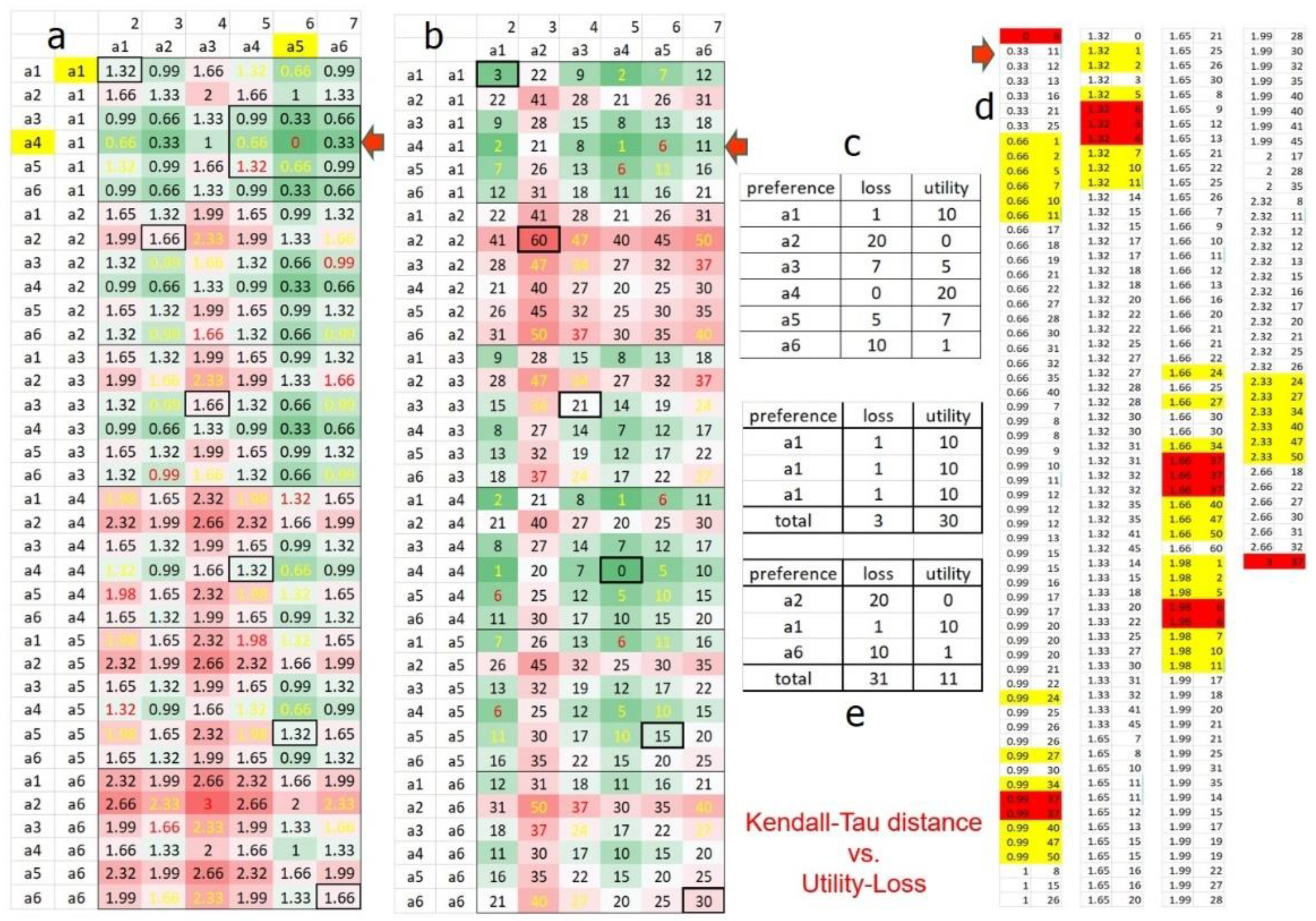
- Kendall Tau Distance. Available online: https://en.wikipedia.org/wiki/Kendall_tau_distance (accessed on 25 May 2022).
- Albano, A.; Plaia, A. Element weighted Kemeny distance for ranking data. Electron. J. Appl. Stat. Anal. 2021, 14, 117–145. [Google Scholar]
- Gong, Z.; Zhang, H.; Forrest, J.; Li, L.; Xu, X. Two consensus models based on the minimum cost and maximum return regarding either all individuals or one individual. Eur. J. Oper. Res. 2015, 240, 183–192. [Google Scholar] [CrossRef]
- Weiss, G. Multiagent Systems. A Modern Approach to Distributed Artificial Intelligence. Massachusetts Institute of Technology, MIT Press USA. Available online: https://uma.ac.ir/files/site1/a_akbari_994c8e8/gerhard_weiss___multiagent_systems___a_modern_approach_to_distributed_artificial_intelligence.pdf (accessed on 1 October 2022).
- Edelman, P.H. The Myth of the Condorcet Winner. Supreme Court Econ. Rev. 2015, 22, 207. [Google Scholar] [CrossRef]
- Allingham, M.; Ventura López, J. La Teoría de la Elección; Una Breve Introducción; Alianza Editorial: Salamanca, España, 2011. [Google Scholar]
- Mahajne, M.; Volij, O. Pairwise consensus and the Borda rule. Math. Soc. Sci. 2022, 116, 17–21. [Google Scholar] [CrossRef]
- Arnostka, N.; Jiri, S. Trust Model for Social Network; Department of Computer Science and Engineering, University of West Bohemia: Pilsen, Czech Republic, 2008. [Google Scholar]
- Kepner, C.H.; Tregoe, B.B. The New Rational Manager: An Updated Edition for a New World; Princeton Research Press: Princeton, NJ, USA, 1997. [Google Scholar]
- Mahajne, M.; Nitzan, S.; Volij, O. Level r consensus and stable social choice. Soc. Choice Welf. 2015, 45, 805–817. [Google Scholar] [CrossRef]
- Yang, Y.; Dimarogonas, D.V.; Hu, X. Opinion consensus under external influences. Syst. Control Lett. J. 2018, 119, 23–30. [Google Scholar] [CrossRef]
- Tian, Y.; Wang, L. Opinion dynamics in social networks with stubborn agents: An issue-based perspective. Automatica 2018, 96, 213–223. [Google Scholar] [CrossRef] [Green Version]
- Hegselmann, R.; Krause, U. Opinion dynamics and bounded confidence models, analysis, and simulation. J. Artif. Soc. Soc. Simul. 2002, 5. Available online: https://www.jasss.org/5/3/2/2.pdf (accessed on 1 October 2022).
- Bredereck, R.; Chen, J.; Finnendahl, U.P.; Niedermeier, R. Stable roommates with narcissistic, single-peaked, and single-crossing preferences. Auton. Agents Multi-Agent Syst. 2020, 34, 1–29. [Google Scholar] [CrossRef]
- Suraj, Z. An introduction to Rough Set Theory and its Applications. ICENCO Cairo Egypt 2004, 3, 27–30. [Google Scholar]
- Burt, G. Possibility, and probability: Value, conflict and choice. In Conflict, Complexity, and Mathematical Social Science; The Open University: Milton Keynes, UK, 2010; Volume 15, Chapter 4; pp. 55–58. [Google Scholar]
- Hoek, W.; Wooldrige , M. Multi-Agent systems. In Foundations of Artificial Intelligence; Handbook of Knowledge Representation; Elsevier. B.V.: Amsterdam, The Netherlands, 2008; Chapter 24; pp. 887–926. [Google Scholar] [CrossRef]
- Truchon, M.; Gordon, S. Statistical comparison of aggregation rules for votes. Math. Soc. Sci. 2009, 57, 199–212. [Google Scholar] [CrossRef]
- Vahid, M.S. Prioritizing Lean Techniques by Employing Multi-Criteria Decision-Making (MCDM): The Case of Coutinho, 2020. Ph.D. Thesis, Department of Marketing, Strategy and Operations, University Institute of Lisboa, Lisbon, Portugal, October 2020; pp. 1–83. [Google Scholar]
- The Dice Roll with a Given Sum Problem, Worlds of Math & Physics. Available online: https://www.lucamoroni.it/the-dice-roll-sum-problem/ (accessed on 6 May 2022).


Publisher’s Note: MDPI stays neutral with regard to jurisdictional claims in published maps and institutional affiliations. |
© 2022 by the authors. Licensee MDPI, Basel, Switzerland. This article is an open access article distributed under the terms and conditions of the Creative Commons Attribution (CC BY) license (https://creativecommons.org/licenses/by/4.0/).
Share and Cite
García-del-Valle-y-Durán, P.; Hernandez-Martinez, E.G.; Fernández-Anaya, G. The Greatest Common Decision Maker: A Novel Conflict and Consensus Analysis Compared with Other Voting Procedures. Mathematics 2022, 10, 3815. https://0-doi-org.brum.beds.ac.uk/10.3390/math10203815
García-del-Valle-y-Durán P, Hernandez-Martinez EG, Fernández-Anaya G. The Greatest Common Decision Maker: A Novel Conflict and Consensus Analysis Compared with Other Voting Procedures. Mathematics. 2022; 10(20):3815. https://0-doi-org.brum.beds.ac.uk/10.3390/math10203815
Chicago/Turabian StyleGarcía-del-Valle-y-Durán, Pedro, Eduardo Gamaliel Hernandez-Martinez, and Guillermo Fernández-Anaya. 2022. "The Greatest Common Decision Maker: A Novel Conflict and Consensus Analysis Compared with Other Voting Procedures" Mathematics 10, no. 20: 3815. https://0-doi-org.brum.beds.ac.uk/10.3390/math10203815