1. Introduction
In farm management, cattle numbers estimation is one of the most critical tasks in asset valuation and pasture management. Precise cattle counts improve the efficiency of farming during assessing assets. It also helps both companies and individuals to reduce unnecessary losses as it detects theft in time [
1]. In practice, cattle counting in farms can be challenging because of different factors, such as cattle’s overlapping [
2], scene transformation [
3], and environmental illumination changing [
4]. The traditional method, e.g., counting by human, is often very time consuming, labour intensive and error-prone [
5].
Vision-based target counting has gained much attention in recent years. Many scenarios have utilised digital image processing methods for target counting, such as dense crowd counting [
6,
7,
8,
9,
10,
11], crop target counting [
12,
13], cell counting [
14], small target counting [
15]. However, visual-based counting technologies have been poorly studied in animal husbandry and are mostly hardware-based methods.
Deep learning has made good progress in recent years for the crowd density estimation problem [
16]. Crowd density estimation aims to obtain a predicted density graph by learning a mapping between the local features of an image and its corresponding density graph. The density graph represents the distribution of the crowd and the number of people at each pixel point. The estimated crowd size is finally obtained by integral and summing the density graphs. In farm management, crowd density estimation based on convolutional neural networks has achieved good performance in chicken [
17] and pineapple flower counting [
18], but the application on cattle counting is still limited.
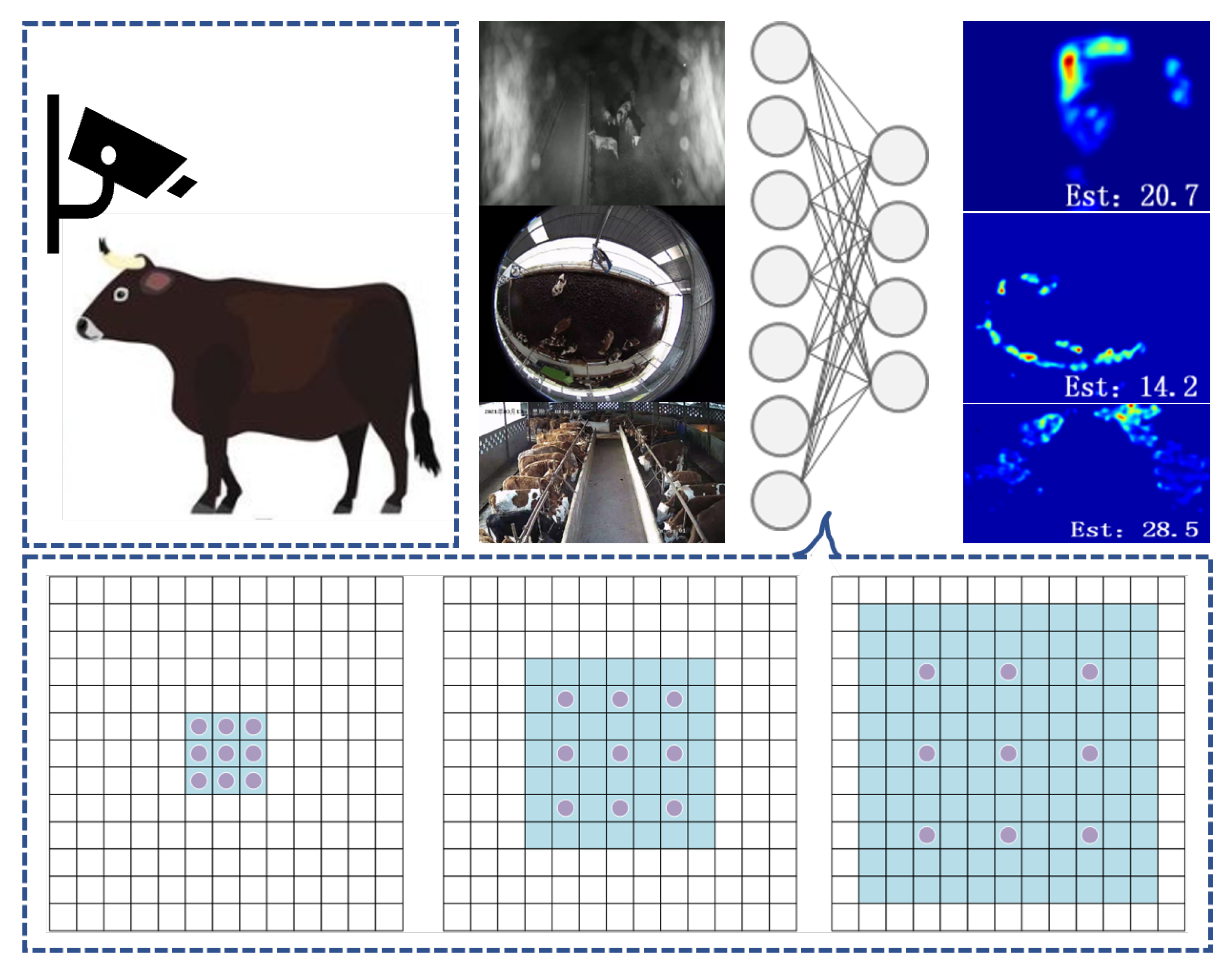
Here we first clarify the problem as three main tasks: (1) uneven distribution of cattle, (2) scale variations caused by perspective, (3) grid effect. Uneven distribution is one of the most significant problems in crowd density estimation. In our collected pasture dataset, cattle distribution varies in different scenes. Scale variations occur on both fish-eye cameras and ordinary cameras; it requires a well-trained model to describe images that are more flexible and robust. Grid effect is inevitable when our model superposes multiple dilated convolutions to analyse the dataset. A high dilation rate can lead to ignorance of critical features, which limits the model performance.
The cattle in image often have very different sizes, ranging from several pixels to tens of pixels. This requires the network to be able to capture a large rang of scales. This paper proposed a multi-scale residual cattle density estimate network called MSRNet, which is built upon the blocks consisting of densely connected dilated convolutional layers. Thus, it can output features having different receptive fields and capture cattle different scales. The MSR block obtains multi-scale receptive fields by using multi-column dilated convolution, and at the same time reduces the grid effect problem caused by continuous dilated convolution, as shown in
Figure 1. So using multiple parallels dilated convolution to extract features is effective for the first two tasks. Using residual structure combined with small dilation rate convolution can help mitigate the grid effect. We summarise our contributions as follows:
Collect a novel herd image dataset in a variety of scenes and conditions.
Train a multi-scale residual cattle density estimate network (MSRNet) for cattle number estimation on both public dataset and collected dataset, and demonstrate the interpretability.
Identify three challenges on this dataset and utilize MSRNet to handle them. Conduct extensive experimentation to demonstrate the performance.
In addition, in contrast to traditional crowd density estimation, crowd datasets are usually labeled with heads of people, while cattle dataset is labeled with body of cattle. Since there is no public cattle dataset, we created a cattle density dataset and verify the effectiveness of our method on this dataset.
The remainder of the paper is structured as follows.
Section 2 reviews existing methods to estimate cattle numbers and relative deep learning methods. In
Section 3, we present details for the proposed methodology, including dataset collection and multi-scale residual cattle density estimation methods. After that, we demonstrate details about our dataset and the experimental results in
Section 4 and discuss possible future works. Finally, we draw important conclusions in
Section 5.
3. Methodology
The fundamental idea of our approach is to deploy an end-to-end multi-scale residual cattle density estimate network with denser scale diversity to cope with the large scale variations and density level differences in both congested and sparse scenes. In this section, we first introduce the generation of density maps, then we describe the architecture of MSRNet, next we explain the loss function, and finally we present the collected dataset.
3.1. Formalization
The goal of our MSRNet model is to generate a density map according to the given input pastures image. The task can be formalized as a mapping: , where X is the input image, D represents the output density map, respectively.
Different from the traditional regression methods that only return a crowd number, the density map provides more information. The image data are labelled with cattle number and position, and the density map will match the target distribution of the ground truth.
The performance of the networks depends heavily on the quality of the supervised data. A high-quality density graph can help improve the performance of the density estimation model in training. Generating a density graph consists of two steps: (1) cattle images annotation, (2) converting the cattle image labels to a cattle density graph. Specifically, let a cow at position
be represented as
. In this way, an annotated image marked as
N cows can be represented as a function below:
In a real image, each cow is of a certain size range and corresponds to a small image area. Setting the value of a pixel to 1 in the annotation file to represent this cow is unreasonable. The Gaussian kernel function is a distributed bell-shaped line, and the closer the coordinates are to the centre, the larger the value, and vice versa. So we use a Gaussian kernel function to replace the pixel value of this central point with a weighted average of the pixel values of the points around it. In this way, the weights of the pixel points within the blur radius add up to 1. This method does not affect the total number of cattle in the resulting density graph but also provides more realistic space location features of each cattle in the picture. For each image
i, the annotated image function is convolved with a Gaussian kernel to obtain the density below:
where
is the density supervisory information and
is the Gaussian covariance.
The single-camera cattle density estimation is challenging because of the occlusion, uneven distribution, scale variations, and grid effect. Here we introduced the collected dataset below and described the multi-scale residual cattle density estimate network. Specifically, we first presented the overall framework of the network. Then, there is a detailed description of the multi-scale residual feature-aware module. In the end, we also discussed the loss function used in this paper.
3.2. Multi-Scale Residual Cattle Density Estimation Methods
3.2.1. MSRNet Structure
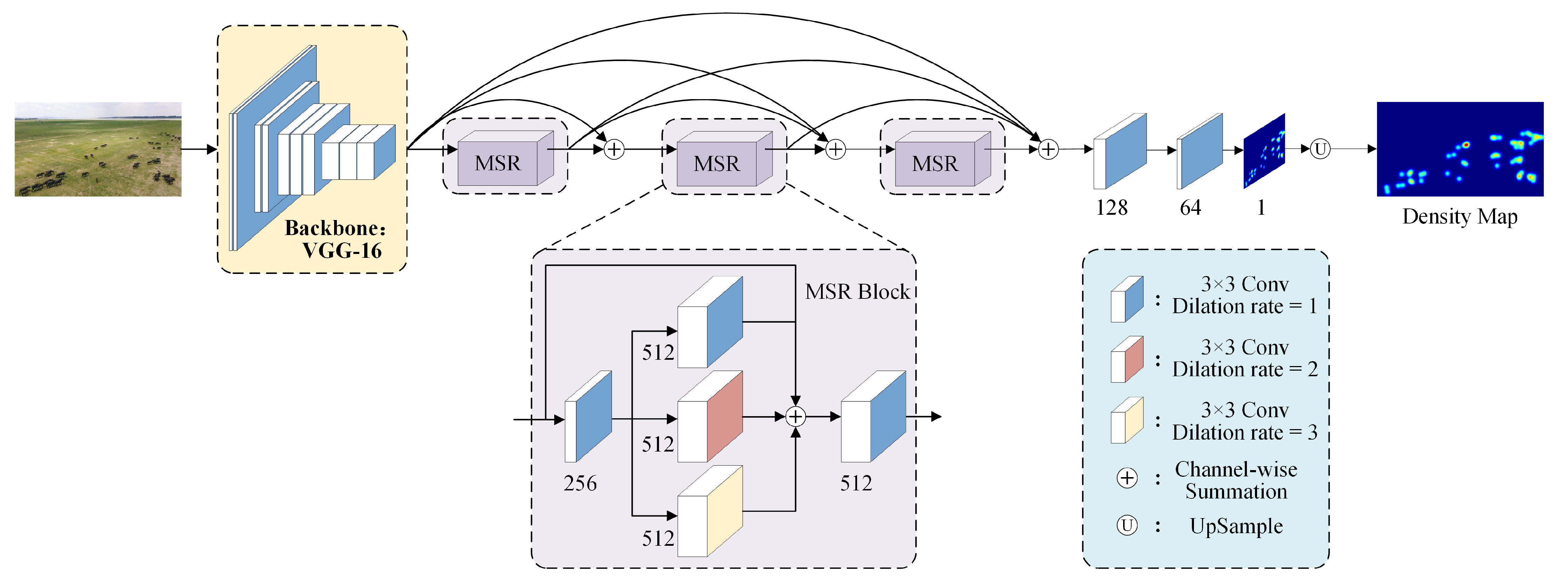
In order to efficiently deal with the uneven distribution of cattle density and large scale variation, a multi-scale residual network (MSRNet) is proposed. The proposed MSRNet structure is illustrated in
Figure 2, which consists of a front-end feature extraction network and three back-end multi-scale feature sensing modules. In particular, the first ten convolutional layers and three pooling layers of the conventional VGG-16 [
28] network are performed here, acting as the front-end feature extraction. The back-end consists of three multi-scale residual feature-aware modules. First, MSRNet apply their multi-scale perceptual fields to extract deeper semantic information, and then a density regression head is applied to obtain the final predicted density graph. The final number of predictions is obtained by integrating the predicted density graph.
3.2.2. Multi-Scale Residual Feature Sensing Module (MSR)
The MSR module is proposed to extract more and deeper semantic information. Each MSR module contains three dilated convolution layers and two conventional convolution layers, as shown in
Figure 2. Compared with the conventional convolution operation, the dilated convolution, proposed by Yu et al. [
29] for solving the image segmentation problem, introduces a “dilation rate” hyperparameter to increase the perceptual field without reducing the image resolution.
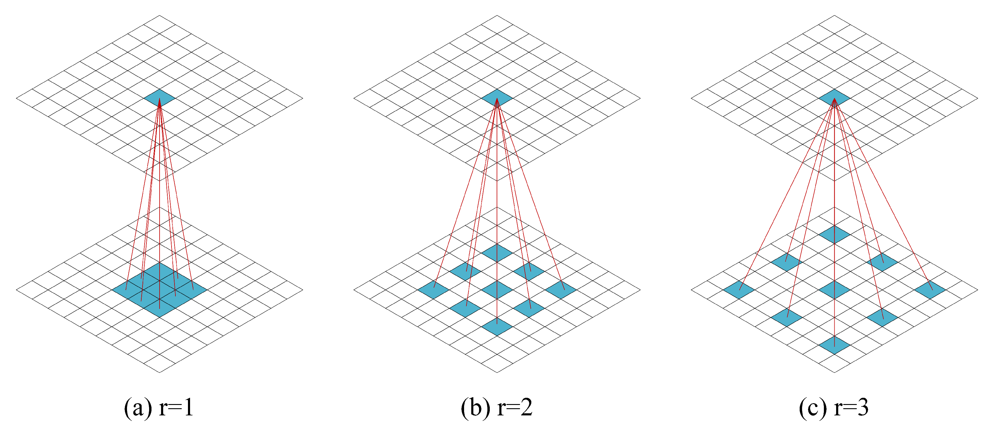
The examples of dilated convolution are shown in
Figure 3. In particular, the dilated convolution expands the receptive field by inserting holes into the normal convolution, the convolution kernel is discontinuous and the features sampled are discrete and uncorrelated. The larger dilation rate will lead to more features being lost. For example, as shown in
Figure 3a, the perceptual field is
when the dilation rate is 1, which is normal convolution, and every pixel in the perceptual field is used. When the dilation rate is 2, the receptive field is
, as shown in
Figure 3b, and only 9 pixels are involved. When the dilation rate is 3, the field is
, as shown in
Figure 3c. The number of pixels used is still 9. Although the dilated convolution reduces the pixels’ usage rate, it would lose more information. The identity shortcut connection between each residual block, is designed to mitigate the pixels’ loss effects.
The channel dimension is first reduced by a convolution, which helps save the subsequent computational effort. The three side-by-side dilated convolutions are used to extract multi-scale features, with a dilation rate of 1, 2 and 3. The dilation rate of 1 indicates the normal convolution, which captures every detail of the image, while the convolutions with a dilation rate of 2 and 3 capture a larger field of sensation and obtain multi-scale features. By means of a constant mapping, the three extracted multi-scale features are then added to the input forming a residual structure. That allows the loss of pixel information caused by the holes to be supplemented to obtain the fused features. Each dilated convolution is followed by a ReLu activation layer. Finally, the fused features are further fused by a convolution. Each module is connected to each other densely, and each layer of the module is tightly connected to the other layers behind it so that information from each layer can be passed to subsequent layers.
3.2.3. Loss Function
Euclidean loss was used to measure the estimation error between the estimated density and the supervised density. Let a set of training sample data be
, in which
. Then the density is
. And the overall mean square error will be the Euclidean loss function as below:
where
N is the batch size during the training. Using the Euclidean loss function to evaluate the prediction gap at the pixel level will ignore the global and local correlation between the estimated density and the true density graph. Therefore, we combined multi-scale density level consistency loss to measure Euclidean loss in both global and local contexts. The density graph is divided into sub-regions of different sizes by a pooling operation, each representing a different density level at a different location. And the network is optimised by constraint with the corresponding true value. The multi-scale density level consistency loss is defined as follows:
where
S denotes the density levels of the divided density graph,
denotes the average pooling level, and
denotes the output size of the average pooling. In this work, the density graph is divided into four levels, and the average pooling output sizes are
,
,
and
. The
size output captures the global information while the remaining three capture the local information. The loss function is defined as follows:
where
represents the Euclidean loss,
is the multi-scale density level consistency loss, and
is the weight hyperparameter that we use to balance the pixel-level and density-level losses. Algorithm 1 provides the pseudo-code of MSRNet.
| Algorithm 1 Multi-scale residual cattle density estimate network (MSRNet) algorithm |
| Input: The input data: and ;
|
| Output: The well-trained MSRNet model ;
|
| 1: | Define the model function and initialize parameters ;
|
| 2: | Define the loss function ;
|
| 3: | The data augmentation from to get ; |
| 4: | fordo |
| 5: | for do |
| 6: | Calculate estimated density ;
|
| 7: | Calculate ground truth ;
|
| 8: | Calculate the ;
|
| 9: | Update to minimize ;
|
| 10: | end for |
| 11: | for do |
| 12: | Calculate estimated density ;
|
| 13: | Calculate ground truth ;
|
| 14: | end for |
| 15: | Calculate the ;
|
| 16: | Calculate the ;
|
| 17: | end for |
| 18: | Save the MSRNet model F;
|
3.3. Herd Image Data Collection
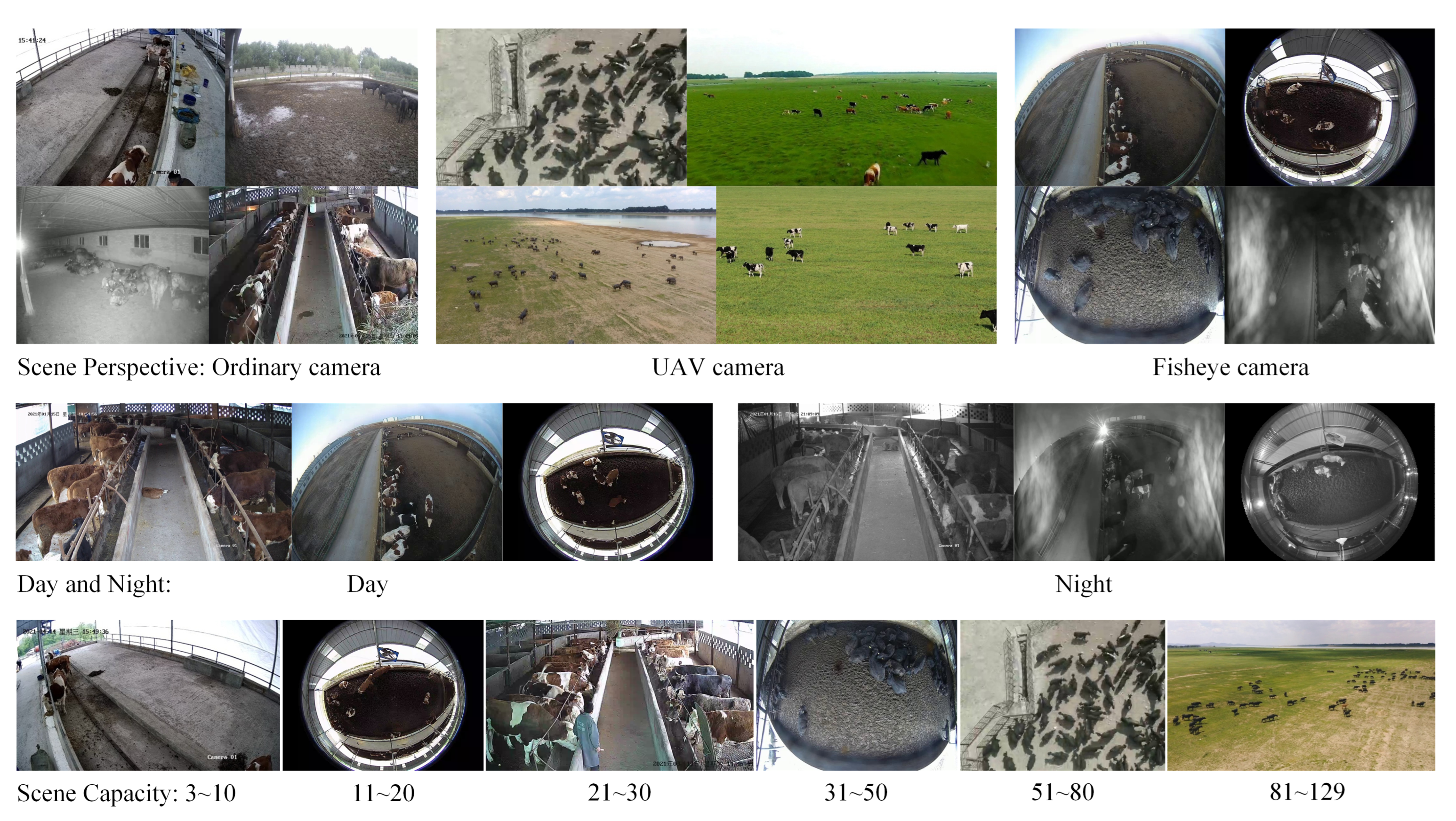
In order to evaluate our proposed MSRNet, a cattle dense dataset is also created. Our proposed dataset is large and contains a variety of scenes and lighting conditions that can represent the real situation of the pasture. Expressly, we set up smart cameras in several pastures of Yibin and Qinghai. It took five months to monitor the daily life of cattle in different periods, seasons, scenarios and weather conditions to get video data. The scenarios include indoor and outdoor cattle pens, and this research includes various types of surveillance cameras, such as fisheye cameras, ordinary cameras and UAV cameras. We intercept video data from different time periods. The intercepted surveillance videos were sampled in real-time and then selected. Data with diverse scenes and significant variations in cattle movement were picked from the dataset. All in all, 850 images were finally selected to build the density estimation dataset, which contains a total of 18,403 cattle. The number of cattle per image varies from 3 to 129 cattle. Some of these samples are shown in
Figure 4. Among them, the data distribution of the above scenarios is shown in
Figure 5. The fisheye cameras accounted for the largest proportion of 500 pictures, and the scene with the number of cattle in the range of 11~20 was the most, including 447 images.
Different from the crowd counting dataset labeling process, the crowd counting datasets use the head as the labeling center during the labeling process, because the position of the head in the picture is obvious and easy to distinguish. Meanwhile, the cattle herd dataset is caused by the complex perspective scene. The center of the label cannot be determined; usually it is the belly of the cow, and in the case of severe occlusion, it is the visible part of the cow, such as the head or the back of the cow. The cattle herd dataset is compared with other population datasets as shown in the
Table 1.
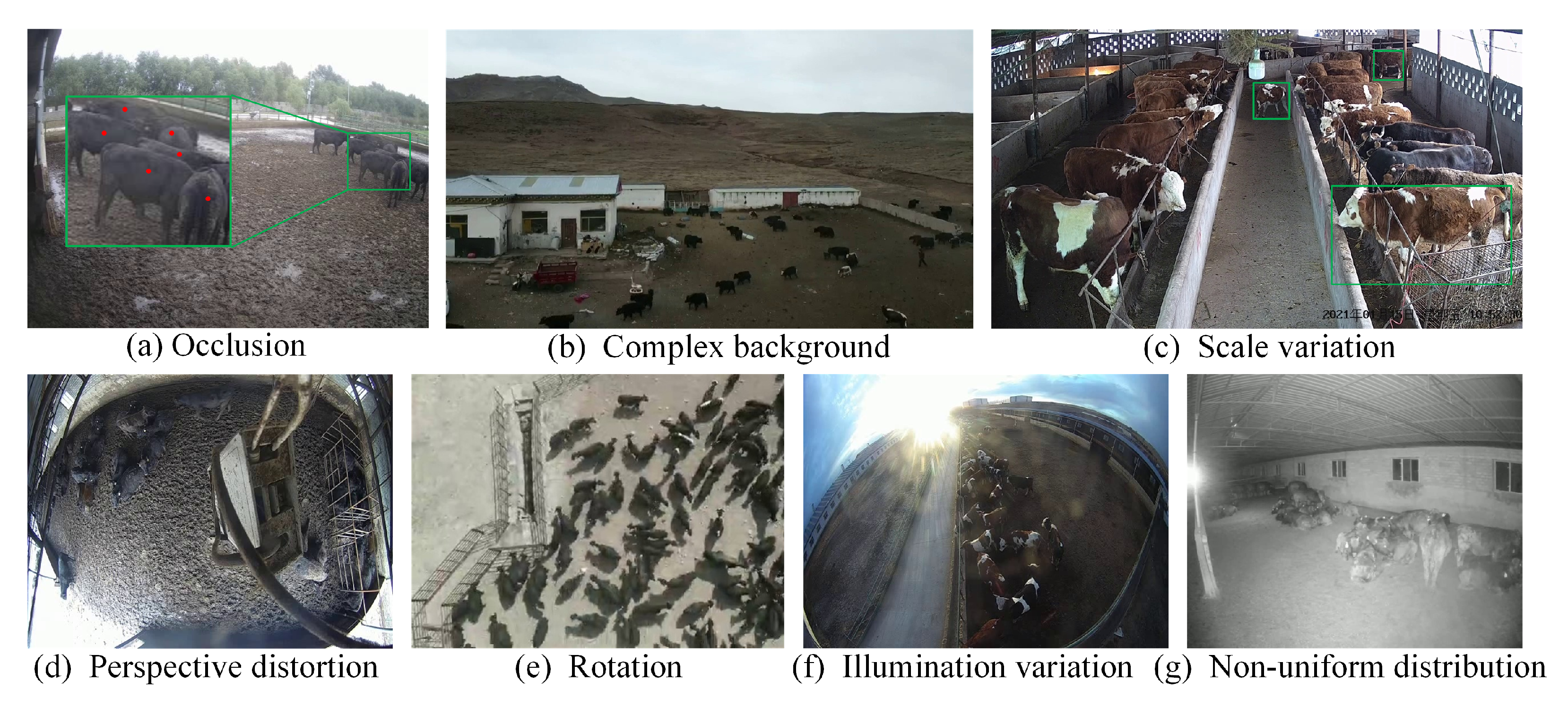
A robust network should have the capability of coping with various complex scenarios. The existence of challenges always brings many difficulties to the models, such as occlusion, complex background, scale variation, perspective distortion, rotation, illumination variation, and non-uniform distribution. Moreover, the scenes of the images are from indoor and outdoor settings, as well as in the wild. It is worth noting that these attributes are not mutually exclusive. In other words, there may exist several attributes in one image. Some samples are shown in
Figure 6.


