Dynamic Path Planning for the Differential Drive Mobile Robot Based on Online Metaheuristic Optimization

Abstract

Mobile robots are relevant dynamic systems in recent applications. Path planning is an essential task for these robots since it allows them to move from one location to another safely and at an affordable cost. Path planning has been studied extensively for static scenarios. However, when the scenarios are dynamic, research is limited due to the complexity and high cost of continuously re-planning the robot’s movements to ensure its safety. This paper proposes a new, simple, reliable, and affordable method to plan safe and optimized paths for differential mobile robots in dynamic scenarios. The method is based on the online re-optimization of the static parameters in the state-of-the-art deterministic path planner Bug0. Due to the complexity of the dynamic path planning problem, a metaheuristic optimization approach is adopted. This approach utilizes metaheuristics from evolutionary computation and swarm intelligence to find the Bug0 parameters when the mobile robot is approaching an obstacle. The proposal is tested in simulation, and well-known metaheuristic methods are compared, including Differential Evolution (DE), the Genetic Algorithm (GA), and Particle Swarm Optimization (PSO). The dynamic planner based on PSO generates paths with the best performances. In addition, the results of the PSO-based planner are compared with different Bug0 configurations, and the former is shown to be significantly better.

1. Introduction

The use of mobile robots is now widespread in a number of applications, including the transport of people and goods [1,2], border surveillance, rescue and monitoring [3,4,5], health and rehabilitation [6], and even entertainment [7]. The growth of this type of robot can be attributed to its ability to operate in extended environments compared to the classic fixed-base robots [8].

Mobile robots can be distinguished by the environment in which they operate (i.e., terrestrial, aquatic, aerial, or hybrid), the type of element that produces their motion (e.g., legs, wheels, caterpillars, propellers, etc.), or the ability to change direction (unidirectional, multidirectional, or omnidirectional) [9]. Among the great diversity of mobile robots, the differential drive one stands out for its ability to move on a plane with only two wheels, the ease with which its movement can be described, the simplicity of its control, its relative low cost, and its universality as it is present in a wide variety of applications [10].

One of the main problems faced by the differential mobile robot and, in general, by any type of mobile robot is path planning [11]. Without loss of generality, path planning refers to the task of getting the mobile robot from an initial configuration (this may include its position and orientation in space) to a final one safely (i.e., avoiding obstacles or threats) and with the least possible cost (e.g., using the least energy, traveling the shortest distance, or with the greatest speed) [12].

Path planning, by its nature, is a complex task [9]. Depending on the features of the robot and its operating environment, this task can be further complicated. Here, it is worth distinguishing two cases: (1) When the operating environment includes static obstacles (i.e., when the obstacles maintain their original configuration over time) and (2) when these obstacles are dynamic (i.e., when the obstacles are moving).

Case (1) has been widely studied in the specialized literature from different approaches. This has given rise to well-known and currently used path planners. In [13], four main types of planners are distinguished. Among these are reactive-computing-based, which can plan the next maneuver quickly and continuously as they receive information from the operating environment. Relevant planners include Bug algorithms [14] and artificial potential fields [15]. For their part, soft-computing-based planners use soft-computing algorithms to approximate paths that meet certain performance criteria. In this field, evolutionary computation and swarm intelligence algorithms [16], neural networks [17], and fuzzy logic [18] stand out. On the other hand, C-space-search-based methods discretize the operation space to reduce the number of possible paths and make planning more efficient. The A* [19] and Rapidly Random Tree (RRT) [20] algorithms are representative of this category. Finally, in the Optimal-Control-Based methods, the path is the solution to the optimal control problem [21].

As for case (2), it adds difficulty to the planning problem inherent to dynamic obstacles. In this case, the methods conceived to solve the path planning problem considering case (1) are not sufficiently effective and require additional mechanisms to handle the environment’s dynamism [13]. Some approaches to handling case (2) that have been successfully tested consist of hybridization of different path planners [22], continuous re-planning of paths as soon as a change in the operating environment is detected [23], or inclusion of new operators in existing planning methods [24]. Thus, many of the planners proposed to date for case (2) are very sophisticated and require advanced theoretical and practical tools to be implemented. Some of these have high computational costs that may be unfeasible, and in many cases, their operation may be limited to conditions that are difficult to meet in practice.

Some recent works regarding cases (1) and (2) are described next. The work in [25] proposes a minimum-time path-planning approach for mobile robots in dynamic environments. For this, the authors establish an optimization problem to find the path points that minimize the realization time, produce a valid speed profile, and avoid collisions. The problem is solved through the Resilient Propagation algorithm periodically, and the resulting paths reduce the number of collisions and time in a simulated soccer game. In [26], an improved variant of the RRT is proposed to handle static scenarios with a mobile robot. The new proposal reduces the complexity of the search trees of the original RRT and produces suitable paths for realistic environments. The research in [27] performs the mobile robot path planning using a pseudo-spectral method to solve an optimal control problem. That method discretizes the path planning problem to transform it into a nonlinear optimization one. The solution to the above problem contains global polynomial approximations of the path for static scenarios. Similarly, the work in [28] transforms the optimal control problem into a nonlinear optimization one and then solves it through the nonlinear trapezoidal collocation programming method. The obtained paths adequately avoid static obstacles and have a reduced length. A multi-agent version of the A-heuristic, a C-space-search algorithm, is proposed in [29] to reduce the time in computing feasible paths for mobile robots in static and dynamic scenarios. A hybrid Genetic Algorithm (GA) is proposed in [30] to solve the path optimization problem with static obstacles. The problem considers the minimization of the path length defined in terms of Bezier curves. As a result, the GA obtains smooth paths for mobile robots. A variant of GA is also used in [31] to solve the path planning problem in dynamic scenarios, this time through a multi-objective optimization approach. The problem consists of finding the best motion command that improves the goal reachability, increases the path smoothness, reduces the realization time, and guarantees the robot’s safety. In [32], the path planning for a mobile robot is performed over the CG-Space, a space conformed by all gravity center positions of the robot considering different terrains. Different approaches, including reactive computing, C-space search, and soft computing, are considered to solve the derived path planning problem. The approach from soft computing based on the Particle Swarm Optimization (PSO) algorithm obtains better paths in terms of smoothness and reduced length. Another work that utilizes soft computing in path planning for static and dynamic scenarios is [33]. In that paper, the grasshopper algorithm is complemented with a sensing system to solve the path optimization problem. The problem considers the maximization of the distance to the obstacles and the minimization of the distance to the goal. Finally, in [34], a soft computing algorithm, the variable-length vector Differential Evolution (DE), is proposed to solve the path planning optimization problem for robots considering static obstacles. In that work, the optimization problem is to find a variable number of points in the path that minimize the length and ensures obstacle avoidance. The obtained results are better than A* and an RRT variant.

As noted, a common thread in many recent works on path planning for mobile robots in static and dynamic environments is formulating an optimization problem. This may be because the desired path requirements can be expressed naturally and explicitly through mathematical language in an optimization problem. Most of the problems addressed in these works are complex due to their features, such as high non-linearity, non-continuity, or non-differentiability, induced by the mobile robot’s behavior or the scenarios’ dynamism. Due to these complications, previous works opt for approximate solution approaches to these problems, many based on soft computing techniques known as metaheuristics, which can provide outstanding results compared with other path-planning methods.

Metaheuristics are computational techniques that can provide high-performance approximate solutions to complex optimization problems at a reasonable computational cost without requiring them to meet specific features [35]. Most metaheuristics are soft computing methods derived from evolutionary computing and swarm intelligence [36], i.e., they are inspired by the behavior of natural systems or phenomena.

Based on the above, this work proposes a new, simple, reliable, and affordable method to plan safe and optimized paths for the differential mobile robot in dynamic scenarios. The method is based on a simple and efficient Bug-type planner known as Bug0 [13]. This proposal re-optimizes the Bug planner online through three well-known metaheuristics: Differential Evolution, the Genetic Algorithm, and Particle Swarm Optimization. This new planner is tested in simulation using a scenario with several moving obstacles and is compared to the original Bug0 algorithm with fixed parameters.

The rest of the paper is organized as follows. Section 2 describes the differential drive mobile robot. Section 3 introduces the features of deterministic path planners with a special focus on Bug methods and Bug0. The proposed dynamic path planner based on the online optimization of a Bug-type method through metaheuristics is developed in Section 4. The experimental details and results are discussed in Section 5. Conclusions are drawn in Section 6.

2. Differential Drive Mobile Robot

The differential drive mobile robot is a mechanical system with the ability to move in the plane $XY$ by using two identical wheels placed on the same axis of rotation. The orientation and position of this robot depend on the difference in the rotation speeds of the two wheels. The above configuration can be described by three generalized coordinates as seen in Figure 1. These coordinates include the position x, y of the robot on the plane, and the angular position $\theta$ measured concerning the axis X.

2.1. Kinematic Model

The kinematic model describes the robot’s motion in terms of the generalized coordinates and the input rotation speeds of the wheels without considering the forces or torques that produce the motion. This model can be utilized to simulate the behavior of the robot. To determine the kinematic model of the differential mobile robot, the geometrical elements that influence its positioning and orientation must be considered. These elements are the radius of the wheels r and the length of the axis separating them L. Thus, this model is derived below.

When both wheels rotate at given speeds, the robot platform travels with tangential velocity v, and rotates with angular speed $\omega$ and radius R around the Instantaneous Center of Rotation ($ICR$). Then, from Figure 1, it is easy to observe that:

$$\begin{array}{cc}\hfill \dot{x}& =vcos\left(\theta \right)\hfill \\ \hfill \dot{y}& =vsin\left(\theta \right)\hfill \\ \hfill \dot{\theta }& =\omega \hfill \end{array}$$

(1)

where $\dot{x}=dx/dt$ and $\dot{y}=dy/dt$ are the components of the velocity v at X and Y, respectively, and $\dot{\theta }=d\theta /dt$ is the rotational speed of the robot, with t as the time.

Both v and $\omega$ in (1) can be considered as the inputs of the robot since they can be expressed in terms of the rotational speeds of the two wheels, as described next.

From Figure 1, the velocity v can be determined as:

$$v=R\omega$$

(2)

Likewise, the tangential velocities $v_l$ and $v_r$ of the wheels can be expressed in terms of R, L, and $\omega$ as:

$$\begin{array}{cc}\hfill v_l& =R_l\omega =\left(R-\frac{L}{2}\right)\omega \hfill \\ \hfill v_r& =R_r\omega =\left(R+\frac{L}{2}\right)\omega \hfill \end{array}$$

(3)

where $R_l$ and $R_r$ are the rotation radius of each wheel with respect to $ICR$.

Solving the equation system given in (3) for $\omega$ and R leads:

$$\begin{array}{cc}\hfill \omega & =\frac{v_r-v_l}{L}\hfill \\ \hfill R& =\frac{L}{2}\left(\frac{v_l+v_r}{v_r-v_l}\right)\hfill \end{array}$$

(4)

Substituting $\omega$ and R in (2) gives:

$$v=\frac{v_r+v_l}{2}$$

(5)

From (4) and (5), it is clear that v and $\omega$ depend on the tangential velocities of the wheels $v_l$ and $v_r$. In turn, the above velocities can be determined if one knows the rotation speeds of the wheels ${\omega }_l$ and ${\omega }_r$ as $v_l=r{\omega }_l$ and $v_r=r{\omega }_r$.

2.2. State-Space Kinematic Model

Simulating the differential mobile robot’s kinematic behavior requires defining the state concept first. The state of a system is a vector with a minimum set of variables that define its behavior for any instant of time. In the case of mechanical systems, including the differential mobile robot, the states that define their kinematic behavior can be given by the generalized coordinates. Therefore, the vector of states for this robot is:

$$z\left(t\right)={[x\left(t\right),y\left(t\right),\theta \left(t\right)]}^T$$

(6)

Based on the above state vector, it is possible to define a state equation as follows:

$$\dot{z}\left(t\right)=f(z,u,t)$$

(7)

where $z\left(t\right)$ is the state vector, $u\left(t\right)$ includes the system inputs (these are $v\left(t\right)$ and $w\left(t\right)$, which allow the differential robot to move), and t is the time.

Thus, the state equation can be obtained using the results from the previous kinematic analysis:

$$\dot{z}=\left[\begin{array}{c}\dot{x}\\ \dot{y}\\ \dot{\theta }\end{array}\right]=\left[\begin{array}{c}vcos\left(\theta \right)\\ vsin\left(\theta \right)\\ \omega \end{array}\right]$$

(8)

2.3. Dynamic Model

The differential robot’s dynamic model describes this system’s behavior in terms of its generalized coordinates and also considers the forces or torques that generate its motion. This model allows for more realistic simulations of the system compared to the kinematic model. The Euler–Lagrange approach, a generalization of Newton’s laws for mechanical systems that requires an analysis of energies [37], was used to obtain this model. This approach requires the formulation of the Lagrangian for mechanical systems:

$$L=K-U$$

(9)

where K and U are, respectively, the system’s total kinetic and potential energies.

Based on the Lagrangian in (9), the equations of motion of a non-holonomic system such as the differential mobile robot can be calculated as [38]:

$$\frac{d}{dt}\left(\frac{\partial L}{\partial {\dot{q}}_i}\right)-\frac{\partial L}{\partial q_i}=f_i-\sum _{j=1}^m{\lambda }_j{a}_{ji}$$

(10)

where $q_i$ is the i-th generalized coordinate in $q={[x,y,\theta ]}^T$, and $f_i$ is its corresponding generalized input torque or force, m is the number of non-holonomic constraints on the robot’s motion, ${\lambda }_j$ is the Lagrange multiplier associated with each constraint, and $a_{ji}$ is the component of the motion constraint for the i-th generalized coordinate.

The total kinetic energy of the robot, due to its translational and rotational motions, can be calculated as:

$$K=\frac{1}{2}m{\dot{x}}^2+\frac{1}{2}m{\dot{y}}^2+\frac{1}{2}{I}_z{\dot{\theta }}^2$$

(11)

where m is the mass of the robot and $I_z$ is its inertia tensor around the vertical rotation axis.

On the other hand, the potential energy of the mobile robot is $U=0$ because it operates in the horizontal plane and is not affected by the acceleration of gravity on Earth.

To determine the robot’s generalized input forces and torques, it is worthwhile to look at Figure 2. As observed in the figure, the forces and torques that move the robot are F and ${\tau }_{\theta }$. The components of these two elements for each generalized coordinate are:

$$\begin{array}{cc}\hfill f_1& =Fcos\left(\theta \right)=\frac{1}{r}\left({\tau }_l+{\tau }_r\right)cos\left(\theta \right)\hfill \end{array}$$

(12)

$$\begin{array}{cc}\hfill f_2& =Fsin\left(\theta \right)=\frac{1}{r}\left({\tau }_l+{\tau }_r\right)sin\left(\theta \right) \hfill \end{array}$$

(13)

$$\begin{array}{cc}\hfill f_3& ={\tau }_{\theta }=\frac{L}{2r}\left({\tau }_r-{\tau }_l\right)\hspace{1em}\hspace{1em}\hspace{1em}\hspace{1em}\hspace{1em} \hfill \end{array}$$

(14)

where ${\tau }_l$ and ${\tau }_r$ are the torques of the right and left wheels, respectively, that generate the tangential forces $F_l=r{\tau }_l$ and $F_r=r{\tau }_r$ in Figure 2. The wheel torques are considered the system inputs.

At this point, it is important to note that the differential mobile robot has only one non-holonomic constraint (i.e., $m=1$) that can be observed in Figure 2. That constraint refers to the fact that the robot cannot move laterally. For this constraint to be satisfied, the lateral velocities must be equal ${\dot{y}}_l^{\prime }={\dot{y}}_r^{\prime }$, or else:

$$-\dot{x}sin\left(\theta \right)+\dot{y}cos\left(\theta \right)=0$$

(15)

in a matrix form:

$$A^T\dot{q}=0$$

(16)

with $A={[a_{11},a_{12},a_{13}]}^T={[-sin\left(\theta \right),cos\left(\theta \right),0]}^T$.

Based on the above, the equations of motion in (10) can be expressed in the closed form observed in (17).

$$M\left(q\right)\ddot{q}=E\left(q\right)u-A^T\left(q\right)\lambda$$

(17)

where:

$$M\left(q\right)=\left[\begin{array}{ccc}m& 0& 0\\ 0& m& 0\\ 0& 0& I_z\end{array}\right]$$

(18)

$$E\left(q\right)=\frac{1}{r}\left[\begin{array}{cc}cos\theta & cos\theta \\ sin\theta & sin\theta \\ \frac{L}{2}& -\frac{L}{2}\end{array}\right]$$

(19)

$$u={[{\tau }_l,{\tau }_r]}^T$$

(20)

and $\lambda$ is the Lagrange multiplier associated with the constraint on (15).

2.4. State-Space Dynamic Model

In the closed-form equation in (17), the system’s physical parameters (e.g., the mass m or the inertia J) can be measured or estimated in some way. However, the same cannot be said for the Lagrange multiplier $\lambda$. This variable can be eliminated if a state vector such as the following is chosen:

$$z\left(t\right)={[x\left(t\right),y\left(t\right),\theta \left(t\right),v\left(t\right),\omega \left(t\right)]}^T$$

(21)

Thus, the equation of state for the differential mobile robot is as follows:

$$\dot{z}=f(z,u,t)=B\left(z\right)+C\left(z\right)u$$

(22)

with:

$$B\left(z\right)={[vcos\left(\theta \right),vsin\left(\theta \right),\omega ,0,0]}^T$$

(23)

$$C\left(z\right)={\left[\begin{array}{ccccc}0& 0& 0& \frac{1}{mr}& \frac{1}{2I_z}\frac{L}{r}\\ 0& 0& 0& \frac{1}{mr}& -\frac{1}{2I_z}\frac{L}{r}\end{array}\right]}^T$$

(24)

$$u={[{\tau }_l,{\tau }_r]}^T$$

(25)

The complete development of the above equation can be found at [39].

2.5. Robot Simulation

State equations such as (8) and (22) are ordinary differential equations whose independent variable is t. If an initial condition $z_0$ (i.e., an initial mobile configuration with an initial position $x_0$, $y_0$, and orientation ${\theta }_0$) is imposed on these differential equations, initial value problems are obtained. When these problems are solved, e.g., through a numerical integration method, the result includes the robot’s predicted future states $z(t+dt)$ after a short time interval $dt$ when the input $u\left(t\right)$ is considered. This prediction simulates the mobile robot for a given time window.

3. Deterministic Path Planning

Without losing generality, path planning is a task that allows taking a mobile robot from an initial configuration to a final one with the lowest possible risk and cost.

The above task is performed by a path planner. Deterministic path planners are algorithms that can always find the same paths under the same operating conditions [40]. This type of planner is effective when dealing with static environments. Moreover, its implementation is relatively simple and low-cost, so it is widely used. Nevertheless, deterministic planners are less effective when a mobile robot operates within a dynamic scenario due to its changing conditions and the unpredictable behaviors of its obstacles.

Among the wide variety of available deterministic path planners, the Bug-type is one of the simplest and most affordable [13].

3.1. Bug-Type Path Planners

Bug-type planners are simple state-of-the-art alternatives as they only require feedback from the environment (via sensors or transducers) and do not require a complete map of it [39], i.e., the path is planned based on the scenario information that they can acquire within a given radius.

The operation of this type of path planner can be summarized in two simple behaviors [39]:

• The mobile robot always moves straight from its current position towards the goal.
• The mobile robot changes its moving direction only when it approaches an obstacle.

Mobile robots using Bug-type algorithms can avoid obstacles and move toward the goal. These algorithms require low memory and processing, and the obtained path is often not optimal, but is generally effective in reaching the final configuration without collision [39].

3.2. The Bug0 Path Planner

Among the Bug-type planners, different variants are distinguished by the complexity of their operations and how they perform the two activities mentioned above. All of them have different benefits and limitations. The simplest of these algorithms is known as Bug0 and has two basic behaviors [39]:

• The robot moves towards the goal until an obstacle is detected or the final configuration is reached. A variable-gain linear speed controller and a fixed-gain angular speed controller are used for this, where the variable gain depends on the distance between the robot and the goal.
• If a nearby obstacle is detected, the robot turns $-\pi /2$ or $\pi /2$ (only one choice) concerning the collision direction and follows the contour of the obstacle until it can follow a straight line to the goal. In this case, fixed-gain linear and angular speed controllers are utilized.

Algorithm 1 describes Bug0. At fixed time intervals while moving the differential mobile robot, Bug0 uses the distance to the nearest obstacle $d_{obs}$, the orientation of the nearest obstacle concerning the robot ${\theta }_{obs}$, the position of the goal ${\xi }_g={[x_g,y_g]}^T$, and the current position and orientation of the robot, respectively $\xi \left(t\right)={[x\left(t\right),y\left(t\right)]}^T$ and $\theta$, to calculate the control inputs v and $\omega$ (linear and angular velocities) that take the robot closer to the goal avoiding obstacles in the path. For this, it is assessed whether the distance to the nearest obstacle is safe enough using an appropriate threshold $\mu$ (line 2). In that case, the robot must steer toward the goal using a variable gain for the linear velocity controller v and a fixed gain for the angular speed controller $\omega$ (lines 3 to 7). The variable gain depends on the distance to the goal. Otherwise, the robot will go around the nearest obstacle using fixed-gain linear and angular speed controllers in the direction ${\theta }_{obs}+s(\pi /2)$, i.e., to the left or right of the obstacle direction (when $s=1$ or $s=-1$, respectively), but always in the same direction (lines 9 to 12). Using the control gains (fixed or variable), Bug0 calculates the inputs v and $\omega$ (lines 14 to 16) that move the robot toward the goal, avoiding obstacles in the path.

Here, it is important to note that the output of Algorithm 1 includes the control inputs v and $\omega$ for the differential mobile robot. During a kinematic simulation, i.e., using the model in (8), v and $\omega$ can be used directly as the inputs to the robot. In the case of a more realistic simulation with the model in (22) or in practice, it is necessary to determine the torques of the two wheels on the robot. This can be achieved using an inverse dynamics controller [41] by solving the system of equations in (22) for ${\tau }_l$ and ${\tau }_r$. Thus, the inverse dynamic control for the differential mobile robot using a linear proportional compensator is:

$$\begin{array}{c}{\tau }_l=k_{pv}{e}_v\frac{mr}{2}-k_{p\omega }{e}_{\omega }\frac{I_{z}r}{L}\\ {\tau }_r=k_{pv}{e}_v\frac{mr}{2}+k_{p\omega }{e}_{\omega }\frac{I_{z}r}{L}\end{array}$$

(26)

where $e_v$ and $e_{\omega }$ are the difference between the tangential and angular velocities calculated by Bug0 and the current robot velocities, with $k_{pv}$ and $k_{p\omega }$ as the proportional control gains.

Algorithm 1: Bug0 path planner

4. Proposed Dynamic Path Planner

As mentioned above, the Bug0 algorithm effectively handles the path planning problem for static scenarios. If the environment is dynamic, Bug0 may encounter some difficulties related to its fixed parameters:

• In this algorithm, when the robot is near an obstacle, it always evades it in the same direction (to the left or to the right, i.e., at $\pm \pi /2$ from the collision direction). Therefore, there may be scenarios where the distance traveled increases, where the robot fails to reach the goal, or where there is a collision with obstacles going to the same place;
• In addition, Bug0 uses a fixed gain control when approaching an obstacle. Consequently, there may be scenarios where the movements generated by the fixed gain control (these could be too slow or too fast) do not allow for evading dynamic obstacles on time.

The proposed dynamic path planning method is based on the Bug0 algorithm for its simplicity and low cost and it aims to address the above difficulties through a metaheuristic online optimization approach. In this sense, it is necessary to formulate a formal dynamic optimization problem whose solution includes the Bug0 parameters that help it handle dynamic scenarios. The problem should be solved continuously, whenever necessary (when a threat is near the robot, i.e., when $d_{obs}<\mu$).

The elements of the dynamic optimization problem and the metaheuristic solution approach are described below.

4.1. Dynamic Optimization Problem

In general, a formal dynamic optimization problem can be defined as follows:

$$\mathbf{min}J(p,t)={[J_1(p,t),J_2(p,t),\dots ,J_m(p,t)]}^T$$

(27)

s.t.:

$$g_i(p,t)\le 0,i=1,2,\dots ,n_g$$

(28)

$$h_j(p,t)=0,j=1,2,\dots ,n_h$$

(29)

The above problem is to find the value of the design variables in the vector p that minimizes the m objective functions in J, as seen in (27). Solutions to this problem can be conditioned by $n_g$ inequality constraints in (28) or $n_h$ equality constraints in (29). The objective functions quantify the fulfillment of different performance indicators. On the other hand, inequality constraints (also known as soft constraints) are conditions that can be met with some degree of slack. Finally, equality constraints (also known as hard constraints) are conditions that must be met exactly. Additionally, the search space, i.e., the possible values that the vector p can acquire, is limited by the box constraints, which include each design variable’s minimum and maximum values.

In a dynamic optimization problem as the one in (27)–(29), the time t introduces dynamism. Thus, at each instant of time, the objective functions and constraints can change their value for the same vector of design variables p.

4.1.1. Design Variables

Since one of the problems of Bug0 lies in its fixed parameters, as described above, it is proposed to use a vector of design variables as follows:

$$p={[s,g_1,g_2]}^T$$

(30)

where s is the direction of avoidance (either left or right by $\pi /2$) in case of detecting a nearby obstacle, and $g_1$, $g_2$ are the gains of the mobile speed controllers (see Algorithm 1).

4.1.2. Objective Function

The objective function must quantify the quality of the paths generated by the differential mobile robot when using a given p.

An essential aspect of path planning is that the paths developed by the mobile robot should be low-cost. This may be related to traveling the greatest possible distance in the shortest time or using the least amount of energy.

Therefore, it is proposed to use the objective function in (31). This function considers the Euclidean distance between the goal position ${\xi }_g={[x_g,y_g]}^T$ and the robot position $\widehat{\xi }(t+hdt)={[\widehat{x}(t+hdt),\widehat{y}(t+hdt)]}^T$ estimated by the kinematic model for the instant $t+hdt$ by using Bug0 with the parameters in p, with h as the future prediction horizon, i.e., the number of future steps of $dt$ that are simulated by the kinematic model.

$$J(p,t)=\sqrt{{(x_g-\widehat{x}(t+hdt))}^2+{(y_g-\widehat{y}(t+hdt))}^2}$$

(31)

Therefore, the dynamic planner will be able to perform a simulation of the robot’s behavior using the kinematic model from its current configuration. The above aims to determine the parameters of Bug0 that best bring it closer to the goal.

4.1.3. Constraints

The operation of the differential mobile robot is limited to collision-free paths with moving obstacles in the environment.

In the dynamic path planning problem, the constraints count the number of collisions the robot could have when using a given vector p in Bug0 within the same prediction horizon h discussed in the previous section. Then, the dynamic optimization problem only considers equality constraints as follows:

$$\begin{array}{cc}\hfill h_j(p,t)& =\left\{\begin{array}{cc}1,\hfill & \mathbf{if}{d}_k(t+ldt)<\frac{L}{2}+\frac{L_k}{2}\hfill \\ 0,\hfill & \mathbf{otherwise}\hfill \end{array},\right.\hfill \\ \hfill j& =1,2,\dots ,n_{obs}h,\hfill \\ \hfill k& =1,2,\dots ,n_{obs},\hfill \\ \hfill l& =1,2,\dots ,h\hfill \end{array}$$

(32)

where $d_k(t+ldt)$ is the Euclidean distance between robot position $\widehat{\xi }(t+ldt)={[\widehat{x}(t+ldt),\widehat{y}(t+ldt)]}^T$ (estimated by the kinematic model for the instant $t+ldt$ by using Bug0 with the parameters in p) and the k-th obstacle location ${\widehat{\xi }}_k(t+ldt)={[{\widehat{x}}_k(t+ldt),{\widehat{y}}_k(t+ldt)]}^T$ (predicted or calculated for the instant $t+ldt$), $L_k$ is the length of the k-th obstacle, and $n_{obs}$ is the number of dynamic obstacles. It is assumed that the location of every dynamic obstacle ${\widehat{\xi }}_k(t+ldt)$ can be predicted or calculated [42,43].

With the above, the planner can simulate the mobile robot’s kinematic behavior and use the positional information of the dynamic obstacles to determine whether a configuration p of the Bug0 algorithm can avoid collisions.

4.2. Solving a Dynamic Optimization Problem

As discussed above, a dynamic optimization problem is one in which the objective function and/or constraints change over time. Typically, there are two ways to solve this type of problem [44]:

• Using an optimizer that solves the problem from scratch each time a change is detected;
• Incorporating additional mechanisms in the optimizer to adapt the solutions found so far without solving the problem from scratch.

The solution approach (1) is adopted in this work to maintain the simplicity of the proposal.

4.3. Metaheuristic Optimizers

The optimization problem in (30)–(32) includes highly nonlinear, discontinuous, and non-differentiable elements, which makes it difficult to solve by traditional search or optimization methods. For this reason, approximate optimization techniques, such as metaheuristics, may be suitable alternatives to find good solutions to this kind of problem [45].

Although a wide variety of metaheuristics are currently available [36], no single one of them is capable of providing the best solutions to all types of optimization problems, according to the No Free Lunch theorems [46]. One way to select the best alternative among these techniques for a specific problem is to do so empirically, by testing different metaheuristics of proven effectiveness. This approach is adopted in this work. Among the available metaheuristics, three alternatives have a proven track record of successful use in various science and engineering contexts. Differential Evolution, the Genetic Algorithm, and Particle Swarm Optimization are these techniques. Many recent metaheuristics are based on the above techniques or propose improvements at an additional computational cost.

The general performance of these three metaheuristic optimizers is described below.

4.3.1. Differential Evolution

Differential Evolution (DE) [47] is a metaheuristic optimization technique inspired by natural evolution. This algorithm has a population of individuals that searches for the approximate solution to a complex optimization problem. DE has several variants, and one of the simplest and most effective is rand/1/bin [48]. The general operation of DE rand/1/bin is described in Algorithm 2. In DE, each D-dimensional vector $p_i={[x_{i_1},p_{i_2},\dots ,p_{i_D}]}^T$, $i=1,2,\dots ,NP$ (also called individual) in a population with $NP$ vectors is used to represent a candidate solution to the optimization problem. At the beginning of the algorithm, the initial population includes individuals randomly generated in the search space delimited by $d_{min}$ and $d_{max}$ (lines 1 and 2). During a maximum of $G_{max}$ generations, each of the base individuals in the current population P generates first a mutant with the rand/1 operator, which uses the scaling factor F and three random individuals from P (lines 5 and 6). Then, the base individual and its mutant are recombined to obtain an offspring through the $bin$ operator and the crossover rate $CR$ (line 7). Finally, the base individual competes with its offspring to determine the fittest solution, which persists in P (line 8). For this, the performance of each individual is measured in terms of their ability to solve the optimization problem. At the end of the last generation, the best individual from the population P is selected as the approximated solution to the optimization problem (lines 10 and 11).

Algorithm 2: Differential Evolution

4.3.2. Genetic Algorithm

As DE, the Genetic Algorithm (GA) is a metaheuristic technique based on natural evolution, but at chromosome level [49]. Currently, several variants of GA have been proposed and are distinguished by the approaches adopted in the evolutionary operations of crossover, mutation, selection, and the codification of the chromosomes. One popular and effective GA, widely used to solve multi-objective optimization problems, is the Non-dominated Sorting Genetic Algorithm II (NSGAII) [50]. The Algorithm 3 describes the operation of a single-objective version of NSGAII referred to as GA only. In the GA in Algorithm 3, the chromosomes are D-dimensional vectors $p_i={[x_{i_1},p_{i_2},\dots ,p_{i_D}]}^T$, $i=1,2,\dots ,NP$ that represent possible solutions to an optimization problem. GA starts with a population with $NP$ chromosomes randomly generated in the search space given by $d_{min}$ and $d_{max}$ (lines 1 and 2). During $G_{max}$ generations, $NP/2$ couples of chromosomes are selected from the population through a binary tournament (line 4). The contestants of each tournament are chosen randomly from the population. Next, each couple of chromosomes can be recombined through the Simulated Binary Crossover (SBX) operator with the distribution index ${\eta }_c$ [51] and based on a given probability $P_c$ (line 5). SBX generates two offspring chromosomes that can be mutated at the given rate $P_m$ through the Polynomial Mutation (PM) operator with the distribution index ${\eta }_m$ [52] (line 6). The resulting new chromosomes are included in the population P (line 7). By the end of each generation, only the $NP$ fittest chromosomes are preserved in the population P (line 8). After the maximum number of generations $G_{max}$ is reached, the best chromosome in the population is taken as the solution to the optimization problem (lines 10 and 11).

Algorithm 3: Genetic Algorithm

4.3.3. Particle Swarm Optimization

Unlike the evolutionary algorithms DE and GA, Particle Swarm Optimization (PSO) is a representative swarm intelligence method. This kind of metaheuristic is inspired by the collaborative nature of species in search of survival [53]. PSO considers a swarm of particles (e.g., individuals of any species) whose positions change over time to find a beneficial location (e.g., with the greatest amount of resources). A universally used variant of PSO considers a swarm with fully connected topology (i.e., each particle knows the others) and assumes that the particles have a memory of their best positions and the best position of the swarm. Furthermore, using a linearly decreasing inertia factor while updating particle positions has been shown to be beneficial in many PSO applications [54]. Algorithm 4 describes the operation of the above PSO variant. In PSO, D-dimensional vectors $p_i={[x_{i_1},p_{i_2},\dots ,p_{i_D}]}^T,i=1,2,\dots ,NP$ represent the position of each particle in a swarm of $NP$. Each position is a candidate solution to the optimization problem. These positions are generated randomly in the search space bounded by $d_{min}$ and $d_{max}$ (lines 1 and 2). In addition, each particle keeps a record of its best-known position (line 3) and the best-known position by the swarm (line 4). At each iteration, PSO updates the velocity of each particle using an inertia weight, its current position, its best-known position (also known as personal best), and the best-known position of the swarm (also known as global best) using the constants $C_1$ and $C_2$ that ponders the local and global knowledge respectively, with $C_1+C_2<4$ (line 8). The inertia weight w starts in a maximum value $w_{max}$ and decreases linearly on each iteration until $w_{min}$ (line 6). The calculated velocity updates the particle position (line 7). Every time a particle position is obtained, the personal and global best positions are updated (lines 10 and 11). When the last iteration $G_{max}$ is reached, the global best position is selected as the solution to the optimization problem.

Algorithm 4: Particle Swarm Optimization

4.4. Additional Considerations on the Metaheuristic Optimizers

The original versions of the aforementioned algorithms consider unconstrained single-objective optimization problems with continuous variables. In this section, we present the aspects that must be considered in the metaheuristic optimizers to be able to handle the dynamic path planning problem for the differential mobile robot.

4.4.1. Handling Hard Constraints

For unconstrained optimization problems, whenever it is necessary to discriminate a solution in DE, GA, or PSO, only the value of the objective function J is considered. In the case of problems with constraints, such as dynamic path planning, it is necessary to incorporate a mechanism that considers the feasibility of the solutions (i.e., the extent to which they comply with the constraints). Deb’s rules mechanism is a simple and efficient alternative to handle constrained problems [55]. For this purpose, the rules first weigh the feasibility and then the optimality when comparing two solutions.

Deb’s feasibility rules establish the following [55]:

• If a feasible solution is compared against a non-feasible solution, then the former is preferred;
• If two feasible solutions are compared, the one with the best objective function value is preferred;
• If two infeasible solutions are compared, the one with the lowest constraint violation sum is preferred.

The constraint violation sum is represented as follows for a dynamic optimization problem:

$$\varphi (p,t)=\sum _{i=1}^{n_g}\max {\left\{0,g_i(p,t)\right\}}^2+\sum _{j=1}^{n_h}\left|h_j(p,t)\right|$$

(33)

The above rules are included in the metaheuristics to handle the constraints of the dynamic path planning problem.

4.4.2. Handling Box Constraints

Another problem faced by these metaheuristics is to ensure that the solutions generated during their operation remain within the search space given by $d_{min}$ and $d_{max}$ (i.e., the box constraints). The metaheuristics used in this work adopt a simple mechanism to handle box constraints. This mechanism consists of regenerating the variable randomly when it exceeds the bounds $d_{min}$ and $d_{max}$:

$$p_{i,j}=\left\{\begin{array}{cc}\hfill p_{i,j},& \mathbf{if}{d}_{min,j}\ge p_{i,j}\ge d_{max,j}\hfill \\ \hfill d_{min,j}+rand(0,1)(d_{max,j}-d_{min,j}),& \mathbf{otherwise}\hfill \end{array}\right.$$

(34)

4.4.3. Handling Mixed Variables

As could be observed in the problem in (30)–(32), the design variables considered are mixed [56]. This is because the control gains $g_1$ and $q_2$ in (30) are continuous, while the avoidance direction $s\in \{-1,1\}$. By their very nature, the metaheuristics considered in this work can handle only continuous variables. However, a simple mechanism is incorporated to handle mixed variables to solve the dynamic planning problem. The mechanism consists of mapping the value of s to the values in the set $\{-1,1\}$ with (35) each time the problem needs to be evaluated or when the solution is used in Bug0.

$$s=\left\{\begin{array}{cc}\hfill 1,& \mathbf{if}s\ge 0\hfill \\ \hfill -1,& \mathbf{otherwise}\hfill \end{array}\right.$$

(35)

5. Experiments and Results

The dynamic path planner described in the previous section is tested in simulation.

5.1. Experiments Details

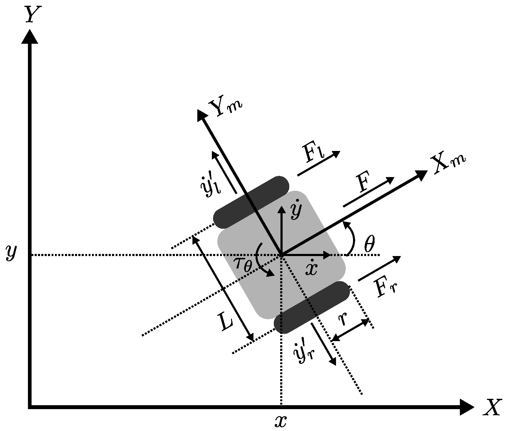
For the experimentation, the robot is simulated with the dynamic model in (22) to provide results closer to reality. In that model, the kinematic parameters of the mobile robot are L = 15 (cm) and r = 2.4 (cm), while the dynamic ones are m = 0.75 (kg) and $I_z$ = 0.001 (kg·m²), as proposed in [39]. The mobile robot simulation is performed using the numerical Euler integration method with a step size $dt$ = 0.03 (s). Additionally, the proportional gains of the inverse dynamics controller in (26) are chosen as $k_{pv}=50$ and $k_{p\omega }=50$ to govern the robot wheels based on the input commands v and $\omega$. On the other hand, the scenario is not bounded and matches the horizontal $XY$ plane. Moreover, the start and goal points are fixed in the scenario. The start point is ${\xi }_0={[0,0]}^T$ (m) and the goal is ${\xi }_g={[4,0]}^T$ (m). The initial orientation of the differential mobile robot is ${\theta }_0=0\left(rad\right)$. Seven dynamic obstacles are considered within the scenario ($n_{obs}=7$), each of them with the same size of the mobile robot, i.e., $L_k=L,k=1,2,\dots ,n_{obs}$. The dynamic behavior of each obstacle in the scenario is described in

Table 1. Dynamic behavior of obstacles in the test scenario for $t\in [0,15]$ (s).

Obstacle	x (m)	y (m)
1	$1.0$	$0.1sin\left(\frac{t}{2}\right)$
2	$2.0+0.2cos\left(\frac{t}{2}\right)$	$-0.2+0.2sin\left(\frac{t}{2}\right)$
3	$3.0$	$0.1cos\left(\frac{t}{2}\right)$
4	$1.0+0.5cos\left(\frac{t}{2}\right)$	$0.25$
5	$3.0+0.5sin\left(\frac{t}{2}\right)$	$-0.25$
6	$2.0+2.0sin\left(2t\right)$	$0.5$
7	$2.0+2.0cos\left(2t\right)$	$-0.5$

. The threshold used in Bug0 is set as $\mu$ = 0.25 (m).

Concerning the dynamic optimization problem, the box constraints used to limit the values of the design variables are as follows: $d_{min}={[0.0,0.0,-1.0]}^T$ and $d_{max}={[1.0,10.0,1.0]}^T$. As for the kinematic simulation of the mobile robot required to make future predictions, a sampling interval $dt$, a prediction horizon $h=10$, and Euler’s numerical integration method are used.

In the case of the metaheuristics DE, GA, and PSO, their parameters are selected based on the suggestions in the specialized literature. The parameters of DE are the scaling factor F generated randomly in $[0.3,0.9]$ at each generation and the crossover rate $CR=0.5$ [48]. In the case of GA, the crossover and mutation probabilities are $P_c=1$ (this value ensures that the same number of evaluations of the optimization problem are always carried out per generation) and $P_m=1/3$, while their distribution indexes are ${\eta }_c=20$ and ${\eta }_m=20$ [50]. Finally, in PSO, the local and global knowledge constants are $C_1=2$ and $C_2=2$, and the bound of the inertia weight are $v_{min}=0.4$ and $v_{max}=0.9$ [54]. The population/swarm size is established as $NP=25$ and the maximum number of generations/iterations as $G_{max}=100$ for all metaheuristics. The above aims to ensure that the computational cost of the optimization can be affordable in possible physical experimentation. The optimization procedure with the metaheuristics is launched when $d_{obs}<\mu$. Since the controller gains are not optimized by DE until the first time that $d_{obs}<\mu$ is fulfilled, then it is used at first the pair of fixed gains $g_1=0.4$ and $g_2=5$ proposed in [39].

All experiments are performed on a conventional personal computer and implemented in C++. The source code can be found at https://dr-rodriguez-molina.com/codes/ (accessed on 12 October 2022).

5.2. Results and Discussion

In order to generate simulation results and obtain sufficient evidence of the proposal’s performance (from now on, D-Bug0), 30 independent runs were performed with each metaheuristic optimizer under the experimental conditions described in the previous section. The versions of D-Bug0 using Differential Evolution, Genetic Algorithm, and Particle Swarm Optimization are named D-Bug0/DE, D-Bug0/GA, and D-Bug0/PSO, respectively.

Table 2. Descriptive statistics on the results of the 30 independent executions with D-Bug0/DE, D-Bug0/GA, and D-Bug0/PSO.

Measure	Indicator	D-Bug0/DE	D-Bug0/GA	D-Bug0/PSO
Path length (m)	Mean	4.0955	4.1085	4.0909
	Std.	0.0044	0.0057	0.0017
	Min.	4.0897	4.0976	4.0887
	Max.	4.1024	4.1183	4.0947
Collisions	Mean	0.0000	0.0000	0.0000
	Std.	0.0000	0.0000	0.0000
	Min.	0.0000	0.0000	0.0000
	Max.	0.0000	0.0000	0.0000
Arrival time (s)	Mean	12.1890	12.2170	12.1860
	Std.	0.0140	0.0129	0.0122
	Min.	12.1800	12.2100	12.1800
	Max.	12.2100	12.2400	12.2100
Speed (m/s)	Mean	0.3360	0.3363	0.3357
	Std.	0.0003	0.0003	0.0003
	Min.	0.3354	0.3356	0.3351
	Max.	0.3365	0.3370	0.3361
Execution time (s)	Mean	3.2064	3.2254	3.1925
	Std.	0.0508	0.0474	0.0390
	Min.	3.1610	3.1700	3.1510
	Max.	3.4260	3.4220	3.3800

shows the summary statistics on the performance of the alternatives D-Bug0/DE, D-Bug0/GA, and D-Bug0/PSO considering different indicators: the total path length, the number of collisions with the dynamic obstacles, the time it took the differential mobile robot to reach the goal, its average speed, and the computational time to process both the proposed path planning algorithm and the simulation. The best results in this table are highlighted in boldface.

Based on Table 2, the proposed dynamic planner D-Bug0 can generate free-collision paths regardless of the adopted metaheuristic and despite the scenario having multiple moving obstacles. This is highly relevant because it could help safeguard the integrity of the actual differential mobile robot in a physical experimental environment to avoid unnecessary repair costs. Concerning the other indicators, significant differences can be noted in the performance of the three dynamic planners. The PSO-based alternative stands out from the others in terms of path length, time to goal, and execution time. On the other hand, D-Bug0/GA helps the mobile robot track the path at the highest speed. In the same table, the small value of the standard deviation, compared to the mean, for all indicators, indicates that the results obtained are very similar in each run, highlighting the reliability of D-Bug0.

Although the results in Table 2 provide an overview of the performance of the different D-Bug0 planners, it is necessary to confirm the results with a non-parametric statistical test due to the stochastic behavior of the metaheuristics, which generates non-normal distributions of results for each group of 30 independent runs [57]. The pairwise Wilcoxon rank-sum test was adopted for this purpose considering a two-sided alternative hypothesis (this establishes that two results distributions have significant differences) and a statistical significance $\alpha =5\%$ (the minimum probability to accept the alternative hypothesis). The results of the Wilcoxon tests are in

Table 3. Pairwise Wilcoxon tests over the results of the 30 independent executions with D-Bug0/DE, D-Bug0/GA, and D-Bug0/PSO.

Measure	Test			${\mathit{R}}_{+}$	${\mathit{R}}_{-}$	p-Value
Path length	D-Bug0/DE	vs.	D-Bug0/GA	464	1	3.7252 × 10${}^{-9}$
	D-Bug0/DE	vs.	D-Bug0/PSO	43	422	2.3666 × 10${}^{-5}$
	D-Bug0/GA	vs.	D-Bug0/PSO	0	465	1.8626 × 10${}^{-9}$
Collisions	D-Bug0/DE	vs.	D-Bug0/GA	0	0	1.0000
	D-Bug0/DE	vs.	D-Bug0/PSO	0	0	1.0000
	D-Bug0/GA	vs.	D-Bug0/PSO	0	0	1.0000
Arrival time	D-Bug0/DE	vs.	D-Bug0/GA	253	0	2.0342 × 10${}^{-5}$
	D-Bug0/DE	vs.	D-Bug0/PSO	48	72	0.4578
	D-Bug0/GA	vs.	D-Bug0/PSO	0	325	4.8413 × 10${}^{-6}$
Speed	D-Bug0/DE	vs.	D-Bug0/GA	81	384	0.0012
	D-Bug0/DE	vs.	D-Bug0/PSO	387	78	0.0009
	D-Bug0/GA	vs.	D-Bug0/PSO	462	3	9.3132 × 10${}^{-9}$
Execution time	D-Bug0/DE	vs.	D-Bug0/GA	310	125	0.0466
	D-Bug0/DE	vs.	D-Bug0/PSO	136.5	328.5	0.0494
	D-Bug0/GA	vs.	D-Bug0/PSO	43	422	0.0001

. This table includes information from the Wilcoxon tests performed for each indicator considered in Table 2. In addition, it describes the test performed and shows the sums of ranks $R_{+}$ and $R_{-}$ (these indicate respectively the number of times the first method outperformed the second and vice versa). The p-value in the last column denotes the probability of accepting the alternative hypothesis and rejecting the null hypothesis (this establishes that two results distributions do not have significant differences). The winner of each pairwise test is shown in boldface.

Table 4. Summary of the pairwise Wilcoxon tests over the results of the 30 independent executions with D-Bug0/DE, D-Bug0/GA, and D-Bug0/PSO.

Measure	D-Bug0/DE	D-Bug0/GA	D-Bug0/PSO
Path length	1	0	2
Collisions	0	0	0
Arrival time	1	0	1
Speed	1	2	0
Execution time	1	0	2
Total wins	4	2	5

summarizes the number of wins for each dynamic planner in the Wilcoxon test. Here, it can be confirmed that D-Bug0/PSO is the best alternative.

Having identified that the best dynamic planner is D-Bug0, it is appropriate to perform a more in-depth analysis of its performance. In this way,

Table 5. Results of D-Bug0/PSO after 30 independent runs.

Run	Path Length (m)	Collisions	Arrival Time (s)	Speed (m/s)	Execution Time (s)
1	4.0904	0	12.1800	0.3358	3.3800
2	4.0901	0	12.1800	0.3358	3.2160
3	4.0925	0	12.1800	0.3360	3.1840
4	4.0925	0	12.2100	0.3352	3.1880
5	4.0893	0	12.1800	0.3357	3.2430
6	4.0897	0	12.1800	0.3358	3.1800
7	4.0912	0	12.1800	0.3359	3.1940
8	4.0894	0	12.1800	0.3357	3.1780
9	4.0924	0	12.2100	0.3352	3.1810
10	4.0947	0	12.2100	0.3354	3.2050
11	4.0887	0	12.1800	0.3357	3.1820
12	4.0908	0	12.1800	0.3359	3.1770
13	4.0933	0	12.2100	0.3352	3.1800
14	4.0893	0	12.1800	0.3357	3.1770
15	4.0945	0	12.2100	0.3353	3.1900
16	4.0900	0	12.1800	0.3358	3.1730
17	4.0891	0	12.1800	0.3357	3.1810
18	4.0898	0	12.1800	0.3358	3.1960
19	4.0927	0	12.1800	0.3360	3.1870
20	4.0904	0	12.1800	0.3358	3.1830
21	4.0901	0	12.1800	0.3358	3.1870
22	4.0898	0	12.1800	0.3358	3.1790
23	4.0888	0	12.1800	0.3357	3.1940
24	4.0898	0	12.1800	0.3358	3.1780
25	4.0894	0	12.1800	0.3357	3.1800
26	4.0936	0	12.1800	0.3361	3.1510
27	4.0902	0	12.1800	0.3358	3.1870
28	4.0923	0	12.1800	0.3360	3.1560
29	4.0897	0	12.1800	0.3358	3.2020
30	4.0919	0	12.2100	0.3351	3.1850
Mean	4.0909	0.0000	12.1860	0.3357	3.1925
STD	0.0017	0.0000	0.0122	0.0003	0.0390
Min	4.0887	0.0000	12.1800	0.3351	3.1510
Max	4.0947	0.0000	12.2100	0.3361	3.3800

shows the results obtained with the D-Bug0/PSO planner corresponding to its 30 independent runs. The first column includes the run number, while the following columns show the path length, collisions, arrival time, speed, and execution time. At the bottom of the table are the summary statistics for each of the above columns. The results in boldface refer to the best results of the 30 runs.

In Table 5, it can be observed that the difference between the minimum and maximum values is less than 0.01 (m) for the path length, approximately 0.01 (s) for the arrival time, and 0.003 (m/s) for the speed, which further denotes that such reliability in spite that D-Bug0/PSO is stochastic. On the other hand, D-Bug0/PSO shows efficiency since all the simulation runs are performed in an acceptable time in proportion to the arrival time. This is observed in the execution time column, where the results do not exceed 3.38 (s). In contrast, the standard deviation for this column is slightly higher in proportion to the mean concerning the rest of the columns. This is because the simulations are conducted on a conventional computer where, in addition, multiple processes derived from the operational functioning are executed at the same time.

At this point, making some observations regarding the execution time is important. One of the aspects that have a greater influence on the execution time in D-Bug0/PSO are the parameters of the PSO optimizer. In particular, $G_{max}$ and $NP$ are the values that have the greatest impact on the time since they determine the number of evaluations of the optimization problem that the metaheuristics utilize (the number of evaluations is $G_{max}NP$). If the number of evaluations is insufficient, the optimizer may find solutions far from optimal. On the other hand, if the number of evaluations is excessive, time may prevent the practical implementation of the planner. One way to evaluate whether the number of evaluations is sufficient is through convergence plots such as those shown in Figure 3. This figure shows the evolution of objective function value J for the best solution in the swarm over the iterations in different optimization processes for an arbitrary run of D-Bug0/PSO. The figure shows that PSO needs about 50 iterations to obtain an unbeatable solution. Considering that, under the proposed experimental conditions, D-Bug0/PSO requires, on average, 96 optimization processes to complete the planning, the processing time for each process is affordable (i.e., less than $dt$), with an adequate budget for problem evaluations. In the case of processing equipment with fewer resources than a conventional PC, the time window to obtain a solution with the metaheuristics can be longer, as it has been observed in other online optimization works [58], however, some parameters of the proposal, such as $\mu$, must also be readjusted.

It is also interesting to observe a sketch of the behavior of D-Bug0/PSO. Figure 4 shows an arbitrary execution of D-Bug0/PSO. This figure plots the complete scenario every 1.5 (s). The red, green, black, and blue circles represent the obstacles, the goal, the robot, and the path’s starting point, respectively. This figure shows how D-Bug0/PSO changes the avoidance direction and robot speed to avoid collisions with dynamic obstacles.

In addition, the results of D-Bug0/PSO are compared with those obtained with the original Bug0 algorithm considering obstacle avoidance always to the left and to the right (from now on, Bug0+ and Bug0−, respectively). The fixed gains for the controllers in Bug0+ and Bug0− are the same as the initial ones for D-Bug0, i.e., $g_1=0.4$ and $g_2=5$.

Table 6. Results of Bug0− after 30 independent runs.

Run	Path Length (m)	Collisions	Arrival Time (s)	Speed (m/s)	Execution Time (s)
1	5.3562	19	19.1100	0.2803	0.0030
2	5.3562	19	19.1100	0.2803	0.0020
3	5.3562	19	19.1100	0.2803	0.0020
4	5.3562	19	19.1100	0.2803	0.0020
5	5.3562	19	19.1100	0.2803	0.0040
6	5.3562	19	19.1100	0.2803	0.0030
7	5.3562	19	19.1100	0.2803	0.0030
8	5.3562	19	19.1100	0.2803	0.0030
9	5.3562	19	19.1100	0.2803	0.0040
10	5.3562	19	19.1100	0.2803	0.0030
11	5.3562	19	19.1100	0.2803	0.0040
12	5.3562	19	19.1100	0.2803	0.0040
13	5.3562	19	19.1100	0.2803	0.0040
14	5.3562	19	19.1100	0.2803	0.0030
15	5.3562	19	19.1100	0.2803	0.0030
16	5.3562	19	19.1100	0.2803	0.0030
17	5.3562	19	19.1100	0.2803	0.0030
18	5.3562	19	19.1100	0.2803	0.0030
19	5.3562	19	19.1100	0.2803	0.0030
20	5.3562	19	19.1100	0.2803	0.0030
21	5.3562	19	19.1100	0.2803	0.0040
22	5.3562	19	19.1100	0.2803	0.0040
23	5.3562	19	19.1100	0.2803	0.0030
24	5.3562	19	19.1100	0.2803	0.0030
25	5.3562	19	19.1100	0.2803	0.0030
26	5.3562	19	19.1100	0.2803	0.0040
27	5.3562	19	19.1100	0.2803	0.0030
28	5.3562	19	19.1100	0.2803	0.0030
29	5.3562	19	19.1100	0.2803	0.0030
30	5.3562	19	19.1100	0.2803	0.0080
Mean	5.3562	19	19.1100	0.2803	0.0033
Std.	0.0000	0	0.0000	0.0000	0.0011
Min.	5.3562	19	19.1100	0.2803	0.0020
Max.	5.3562	19	19.1100	0.2803	0.0080

and

Table 7. Results of Bug0+ after 30 independent runs.

Run	Path Length (m)	Collisions	Arrival Time (s)	Speed (m/s)	Execution Time (s)
1	5.0425	16	16.3500	0.3084	0.0010
2	5.0425	16	16.3500	0.3084	0.0030
3	5.0425	16	16.3500	0.3084	0.0030
4	5.0425	16	16.3500	0.3084	0.0020
5	5.0425	16	16.3500	0.3084	0.0020
6	5.0425	16	16.3500	0.3084	0.0020
7	5.0425	16	16.3500	0.3084	0.0030
8	5.0425	16	16.3500	0.3084	0.0030
9	5.0425	16	16.3500	0.3084	0.0030
10	5.0425	16	16.3500	0.3084	0.0030
11	5.0425	16	16.3500	0.3084	0.0030
12	5.0425	16	16.3500	0.3084	0.0030
13	5.0425	16	16.3500	0.3084	0.0030
14	5.0425	16	16.3500	0.3084	0.0020
15	5.0425	16	16.3500	0.3084	0.0030
16	5.0425	16	16.3500	0.3084	0.0030
17	5.0425	16	16.3500	0.3084	0.0030
18	5.0425	16	16.3500	0.3084	0.0030
19	5.0425	16	16.3500	0.3084	0.0030
20	5.0425	16	16.3500	0.3084	0.0030
21	5.0425	16	16.3500	0.3084	0.0030
22	5.0425	16	16.3500	0.3084	0.0030
23	5.0425	16	16.3500	0.3084	0.0030
24	5.0425	16	16.3500	0.3084	0.0030
25	5.0425	16	16.3500	0.3084	0.0030
26	5.0425	16	16.3500	0.3084	0.0030
27	5.0425	16	16.3500	0.3084	0.0020
28	5.0425	16	16.3500	0.3084	0.0030
29	5.0425	16	16.3500	0.3084	0.0030
30	5.0425	16	16.3500	0.3084	0.0030
Mean	5.0425	16	16.3500	0.3084	0.0028
Std.	0.0000	0	0.0000	0.0000	0.0005
Min.	5.0425	16	16.3500	0.3084	0.0010
Max.	5.0425	16	16.3500	0.3084	0.0030

include the results obtained with Bug0− and Bug0+ (i.e., Bug0 with fixed parameters and different obstacle avoidance directions), respectively, after 30 independent runs under the same experimental conditions as D-Bug0/PSO. The first column of these tables shows the number of the run, and the following columns show the travel distance, the number of times the robot collided with the dynamic obstacles, the time it took for the robot to reach the goal, the speed and the time it took for the computer to process each variant of the Bug0 algorithm as well as the simulation. As in Table 5, the lower part of these two tables shows the same statistical measures for each column, and, similarly, the best results are shown in boldface.

Table 6 and Table 7 show that the standard deviation is zero for path length, arrival time, and speed, highlighting the deterministic behavior of the Bug0 algorithms. Therefore, the same results of these columns are always observed in each of the 30 independent runs of the Bug0 algorithms. Small variations in execution time values are attributed to other tasks executed in the computer’s operating system. On the other hand, one of the most important findings in these two tables is that the paths generated by Bug0+ and Bug0− always collide with dynamic obstacles. In the case of Bug0−, Table 6 shows that the number of collisions is 19, while in the case of Bug0−, Table 7 indicates it is 16. The difference between the number of collisions is due to the fixed direction in which Bug0+ and Bug0− avoid obstacles. The above results indicate that although the null variation in the results of the runs could be desirable, the generated paths do not meet the objective of collision avoidance and may lead to additional costs during physical testing. For this reason, Bug0 with fixed parameters may not be suitable for path planning in dynamic environments.

Based on Table 5, Table 6 and Table 7, it can be noted that the paths generated by D-Bug0/PSO have, in all cases, reduced path lengths, collisions, and arrival times, and consequently, higher speed values. Based on the above, the paths generated by D-Bug0/PSO are better than those of the original Bug0 planning method. In particular, the fact that the number of collisions in the paths generated by D-Bug0 is zero, while in the paths obtained by Bug0+ and Bug0− it is different, indicates a great advantage of the first method since it can lead to significant savings in robot damage costs in a real scenario. Therefore, after observing the data yielded by the path planners, the high efficiency of the D-Bug0/PSO becomes clear since it obtains better results in all the aspects listed in the Table 5, Table 6 and Table 7, except for the simulation execution time, although the last one is still affordable for eventual experimentation with the physical device.

Finally, Figure 5 and Figure 6 describe the behavior of an arbitrary execution of Bug0− and Bug0+, respectively. These figures include plots of the full scenario every 1.5 (s). The red, green, black, and blue circles represent the obstacles, the goal, the differential mobile robot, and the start of the path, respectively. These figures show how the Bug0 path planner tries (and sometimes fails) to avoid dynamic obstacles by changing the robot’s direction to the left (for Bug0+) or right (for Bug0−) of the potential collision point, even when it might not be the most suitable direction. Moreover, it is observed that, for some obstacles, the speed with which the robot moves, related to the fixed gains $g_1$ and $g_2$, is adequate.

6. Conclusions and Future Work

Path planning is an essential task for the differential mobile robot. This task is complex due to the environment features and the robot’s behavior. Planning is harder when the environment is dynamic and deterministic planners may fail to obtain safe and well-performing alternatives. Nevertheless, proposed advanced methods can resolve this kind of scenario, but their implementation complexity and cost may not be suitable for all applications.

For this reason, the proposed path planning method combines the performance of the deterministic planner Bug0 and metaheuristic techniques to optimize it in achieving optimized and collision-free paths with an affordable computational cost. In this sense, it is observed that Bug0 is effective in static scenarios where obstacles can always be avoided in the same direction. When the scenarios are dynamic, Bug0 may collide since it cannot predict a future interaction between the moving obstacles and the robot. Therefore, the proposal includes a predictive stage, which allows the planner to estimate the robot’s behavior within a future time window and thus determine the best speed control parameters and avoidance direction. To this end, three well-known metaheuristics, including Differential Evolution, the Genetic Algorithm, and Particle Swarm Optimization, are implemented in the proposal to test different combinations of the above values and determine the alternative that allows the robot to approach the goal without colliding.

Based on the results obtained in the simulation, the dynamic planner based on PSO (D-Bug0/PSO) obtains the best collision-free paths with reduced length and arrival time. Likewise, the computational time required by the proposal is affordable and can be used in a physical prototype. Compared to the original Bug0 with fixed parameters, D-Bug0/PSO is significantly better since the former caused the robot to collide several times and increases the path length due to its deterministic behavior.

Future work intends to implement a method to predict the paths of dynamic obstacles and use their information within the planner instead of assuming that their behaviors are known. In addition, online variants of the metaheuristics used are contemplated to avoid starting each optimization process from scratch and reduce computational time. This research can be tested with a physical object by managing these limitations.

References

1. Morales, Y.; Miyashita, T.; Hagita, N. Social robotic wheelchair centered on passenger and pedestrian comfort. Robot. Auton. Syst. 2017, 87, 355–362. [Google Scholar] [CrossRef]
2. Yamashita, A.; Arai, T.; Ota, J.; Asama, H. Motion planning of multiple mobile robots for Cooperative manipulation and transportation. IEEE Trans. Robot. Autom. 2003, 19, 223–237. [Google Scholar] [CrossRef] [Green Version]
3. Paola, D.D.; Milella, A.; Cicirelli, G.; Distante, A. An Autonomous Mobile Robotic System for Surveillance of Indoor Environments. Int. J. Adv. Robot. Syst. 2010, 7, 8. [Google Scholar] [CrossRef]
4. Murphy, R.R.; Kravitz, J.; Stover, S.L.; Shoureshi, R. Mobile robots in mine rescue and recovery. IEEE Robot. Autom. Mag. 2009, 16, 91–103. [Google Scholar] [CrossRef]
5. Matveev, A.S.; Wang, C.; Savkin, A.V. Real-time navigation of mobile robots in problems of border patrolling and avoiding collisions with moving and deforming obstacles. Robot. Auton. Syst. 2012, 60, 769–788. [Google Scholar] [CrossRef]
6. Bolmsjo, G.; Neveryd, H.; Eftring, H. Robotics in rehabilitation. IEEE Trans. Rehabil. Eng. 1995, 3, 77–83. [Google Scholar] [CrossRef]
7. Dieter Schraft, R.; Graf, B.; Traub, A.; John, D. A mobile robot platform for assistance and entertainment. Ind. Robot Int. J. 2001, 28, 29–35. [Google Scholar] [CrossRef] [Green Version]
8. Wang, Y.; Lang, H.; de Silva, C.W. A Hybrid Visual Servo Controller for Robust Grasping by Wheeled Mobile Robots. IEEE/ASME Trans. Mech. 2010, 15, 757–769. [Google Scholar] [CrossRef]
9. Rubio, F.; Valero, F.; Llopis-Albert, C. A review of mobile robots: Concepts, methods, theoretical framework, and applications. Int. J. Adv. Robot. Syst. 2019, 16, 1729881419839596. [Google Scholar] [CrossRef] [Green Version]
10. Ben Jabeur, C.; Seddik, H. Design of a PID optimized neural networks and PD fuzzy logic controllers for a two-wheeled mobile robot. Asian J. Control 2021, 23, 23–41. [Google Scholar] [CrossRef]
11. Hossain, M.A.; Ferdous, I. Autonomous robot path planning in dynamic environment using a new optimization technique inspired by bacterial foraging technique. Robot. Auton. Syst. 2015, 64, 137–141. [Google Scholar] [CrossRef]
12. Bergman, K.; Ljungqvist, O.; Axehill, D. Improved Path Planning by Tightly Combining Lattice-Based Path Planning and Optimal Control. IEEE Trans. Intell. Veh. 2021, 6, 57–66. [Google Scholar] [CrossRef]
13. Sánchez-Ibáñez, J.R.; Pérez-del Pulgar, C.J.; García-Cerezo, A. Path Planning for Autonomous Mobile Robots: A Review. Sensors 2021, 21, 7898. [Google Scholar] [CrossRef]
14. Lumelsky, V.J.; Stepanov, A.A. Path-planning strategies for a point mobile automaton moving amidst unknown obstacles of arbitrary shape. Algorithmica 1987, 2, 403–430. [Google Scholar] [CrossRef] [Green Version]
15. Warren, C. Global path planning using artificial potential fields. In 1989 IEEE International Conference on Robotics and Automation; IEEE Computer Society: Los Alamitos, CA, USA, 1989; pp. 316–321. [Google Scholar] [CrossRef]
16. Aghababa, M.P.; Amrollahi, M.H.; Borjkhani, M. Application of GA, PSO, and ACO algorithms to path planning of autonomous underwater vehicles. J. Mar. Sci. Appl. 2012, 11, 378–386. [Google Scholar] [CrossRef]
17. Glasius, R.; Komoda, A.; Gielen, S.C. Neural Network Dynamics for Path Planning and Obstacle Avoidance. Neural Netw. 1995, 8, 125–133. [Google Scholar] [CrossRef]
18. Pandey, A.; Sonkar, R.K.; Pandey, K.K.; Parhi, D.R. Path planning navigation of mobile robot with obstacles avoidance using fuzzy logic controller. In Proceedings of the 2014 IEEE 8th International Conference on Intelligent Systems and Control (ISCO), Coimbatore, India, 10–11 January 2014; pp. 39–41. [Google Scholar] [CrossRef]
19. Hart, P.E.; Nilsson, N.J.; Raphael, B. A Formal Basis for the Heuristic Determination of Minimum Cost Paths. IEEE Trans. Syst. Sci. Cybern. 1968, 4, 100–107. [Google Scholar] [CrossRef]
20. LaValle, S.M. Rapidly-Exploring Random Trees: A New Tool for Path Planning; Iowa State University: Ames, IA, USA, 1998. [Google Scholar]
21. Martin, C.; Sun, S.; Egerstedt, M. Optimal control, statistics and path planning. Math. Comput. Model. 2001, 33, 237–253. [Google Scholar] [CrossRef]
22. Sangeetha, V.; Krishankumar, R.; Ravichandran, K.S.; Cavallaro, F.; Kar, S.; Pamucar, D.; Mardani, A. A Fuzzy Gain-Based Dynamic Ant Colony Optimization for Path Planning in Dynamic Environments. Symmetry 2021, 13, 280. [Google Scholar] [CrossRef]
23. Stentz, A. Optimal and efficient path planning for partially-known environments. In International Conference on Robotics and Automation; Springer: Boston, MA, USA, 1994; Volume 4, pp. 3310–3317. [Google Scholar] [CrossRef]
24. Ge, S.S.; Cui, Y.J. Dynamic Motion Planning for Mobile Robots Using Potential Field Method. Auton. Robots 2002, 13, 207–222. [Google Scholar] [CrossRef]
25. Okuyama, I.F.; Maximo, M.R.O.A.; Afonso, R.J.M. Minimum-Time Trajectory Planning for a Differential Drive Mobile Robot Considering Non-slipping Constraints. J. Control Autom. Electr. Syst. 2021, 32, 120–131. [Google Scholar] [CrossRef]
26. Wang, J.; Li, B.; Meng, M.Q.H. Kinematic Constrained Bi-directional RRT with Efficient Branch Pruning for robot path planning. Expert Syst. Appl. 2021, 170, 114541. [Google Scholar] [CrossRef]
27. Mao, R.; Gao, H.; Guo, L. Optimal Motion Planning for Differential Drive Mobile Robots based on Multiple-Interval Chebyshev Pseudospectral Methods. Robotica 2021, 39, 391–410. [Google Scholar] [CrossRef]
28. Mao, R.; Gao, H.; Guo, L. Optimal motion planning of differential-drive mobile robots based on trapezoidal collocation method. J. Phys. Conf. Ser. 2019, 1341, 052007. [Google Scholar] [CrossRef]
29. Gia Luan, P.; Thinh, N.T. Real-Time Hybrid Navigation System-Based Path Planning and Obstacle Avoidance for Mobile Robots. Appl. Sci. 2020, 10, 3355. [Google Scholar] [CrossRef]
30. Luan, P.G.; Thinh, N.T. Hybrid genetic algorithm based smooth global-path planning for a mobile robot. Mech. Based Des. Struct. Mach. 2021, 1–17. [Google Scholar] [CrossRef]
31. Cheng, K.P.; Mohan, R.E.; Khanh Nhan, N.H.; Le, A.V. Multi-Objective Genetic Algorithm-Based Autonomous Path Planning for Hinged-Tetro Reconfigurable Tiling Robot. IEEE Access 2020, 8, 121267–121284. [Google Scholar] [CrossRef]
32. Katiyar, S.; Dutta, A. Comparative analysis on path planning of ATR using RRT*, PSO, and modified APF in CG-Space. Proc. Inst. Mech. Eng. Part C J. Mech. Eng. Sci. 2022, 236, 5663–5677. [Google Scholar] [CrossRef]
33. Elmi, Z.; Önder Efe, M. Online path planning of mobile robot using grasshopper algorithm in a dynamic and unknown environment. J. Exp. Theor. Artif. Intell. 2021, 33, 467–485. [Google Scholar] [CrossRef]
34. Rodríguez-Molina, A.; Solís-Romero, J.; Villarreal-Cervantes, M.G.; Serrano-Pérez, O.; Flores-Caballero, G. Path-Planning for Mobile Robots Using a Novel Variable-Length Differential Evolution Variant. Mathematics 2021, 9, 357. [Google Scholar] [CrossRef]
35. Reeves, C.R. (Ed.) Modern Heuristic Techniques for Combinatorial Problems; John Wiley & Sons, Inc.: Hoboken, NJ, USA, 1993. [Google Scholar]
36. Bansal, J.C.; Singh, P.K.; Pal, N.R. Evolutionary and Swarm Intelligence Algorithms; Springer: Cham, Switzerland, 2019; Volume 779. [Google Scholar]
37. Ogata, K. System Dynamics/Katsuhiko Ogata, 4th ed.; Pearson/Prentice Hall: Upper Saddle River, NJ, USA, 2004. [Google Scholar]
38. Greiner, W. Lagrange Equation for Nonholonomic Constraints. In Classical Mechanics: Systems of Particles and Hamiltonian Dynamics; Springer: Berlin/Heidelberg, Germany, 2010; pp. 301–310. [Google Scholar] [CrossRef]
39. Klancar, G.; Zdesar, A.; Blazic, S.; Skrjanc, I. Wheeled Mobile Robotics: From Fundamentals towards Autonomous Systems; Butterworth-Heinemann: Oxford, UK, 2017. [Google Scholar]
40. Tam, C.; Bucknall, R. Cooperative path planning algorithm for marine surface vessels. Ocean Eng. 2013, 57, 25–33. [Google Scholar] [CrossRef]
41. Pedapati, P.K.; Pradhan, S.K.; Kumar, S. Kinematic Control of an Autonomous Ground Vehicle Using Inverse Dynamics Controller. In Advances in Smart Grid Automation and Industry 4.0; Reddy, M.J.B., Mohanta, D.K., Kumar, D., Ghosh, D., Eds.; Springer: Singapore, 2021; pp. 313–324. [Google Scholar]
42. Peng, F.; Zheng, L.; Duan, Z.; Xia, Y. Multi-Objective Multi-Learner Robot Trajectory Prediction Method for IoT Mobile Robot Systems. Electronics 2022, 11, 2094. [Google Scholar] [CrossRef]
43. Wang, C.; Ma, L.; Li, R.; Durrani, T.S.; Zhang, H. Exploring Trajectory Prediction Through Machine Learning Methods. IEEE Access 2019, 7, 101441–101452. [Google Scholar] [CrossRef]
44. Peng, X.; Gao, X.; Yang, S. Environment identification-based memory scheme for estimation of distribution algorithms in dynamic environments. Soft Comput. 2011, 15, 311–326. [Google Scholar] [CrossRef] [Green Version]
45. Xiong, N.; Molina, D.; Ortiz, M.L.; Herrera, F. A Walk into Metaheuristics for Engineering Optimization: Principles, Methods and Recent Trends. Int. J. Comput. Intell. Syst. 2015, 8, 606–636. [Google Scholar] [CrossRef] [Green Version]
46. Wolpert, D.; Macready, W. No free lunch theorems for optimization. IEEE Trans. Evol. Comput. 1997, 1, 67–82. [Google Scholar] [CrossRef]
47. Storn, R.; Price, K. Differential Evolution—A Simple and Efficient Heuristic for global Optimization over Continuous Spaces. J. Glob. Optim. 1997, 11, 341–359. [Google Scholar] [CrossRef]
48. Mezura-Montes, E.; Velázquez-Reyes, J.; Coello Coello, C.A. A Comparative Study of Differential Evolution Variants for Global Optimization. In Proceedings of the GECCO ’06—8th Annual Conference on Genetic and Evolutionary Computation, Seattle, WA, USA, 8–12 July 2006; Association for Computing Machinery: New York, NY, USA, 2006; pp. 485–492. [Google Scholar] [CrossRef] [Green Version]
49. Goldberg, D.E. Genetic Algorithms in Search, Optimization and Machine Learning, 1st ed.; Addison-Wesley Longman Publishing Co., Inc.: Boston, MA, USA, 1989. [Google Scholar]
50. Deb, K.; Pratap, A.; Agarwal, S.; Meyarivan, T. A fast and elitist multiobjective genetic algorithm: NSGA-II. IEEE Trans. Evol. Comput. 2002, 6, 182–197. [Google Scholar] [CrossRef] [Green Version]
51. Deb, K.; Agrawal, R.B. Simulated binary crossover for continuous search space. Complex Syst. 1995, 9, 115–148. [Google Scholar]
52. Deb, K.; Deb, D. Analysing mutation schemes for real-parameter genetic algorithms. Int. J. Artif. Intell. Soft Comput. 2014, 4, 1–28. [Google Scholar] [CrossRef]
53. Kennedy, J.; Eberhart, R. Particle swarm optimization. In Proceedings of the ICNN’95—International Conference on Neural Networks, Perth, WA, Australia, 27 November–1 December 1995; Volume 4, pp. 1942–1948. [Google Scholar] [CrossRef]
54. Shi, Y.; Eberhart, R. Empirical study of particle swarm optimization. In Proceedings of the 1999 Congress on Evolutionary Computation-CEC99 (Cat. No. 99TH8406), Washington, DC, USA, 6–9 July 1999; Volume 3, pp. 1945–1950. [Google Scholar] [CrossRef]
55. Deb, K. An efficient constraint handling method for genetic algorithms. Comput. Methods Appl. Mech. Eng. 2000, 186, 311–338. [Google Scholar] [CrossRef]
56. Wang, F.; Zhang, H.; Zhou, A. A particle swarm optimization algorithm for mixed-variable optimization problems. Swarm Evol. Comput. 2021, 60, 100808. [Google Scholar] [CrossRef]
57. Derrac, J.; García, S.; Molina, D.; Herrera, F. A practical tutorial on the use of nonparametric statistical tests as a methodology for comparing evolutionary and swarm intelligence algorithms. Swarm Evol. Comput. 2011, 1, 3–18. [Google Scholar] [CrossRef]
58. Rodríguez-Molina, A.; Villarreal-Cervantes, M.G.; Serrano-Pérez, O.; Solís-Romero, J.; Silva-Ortigoza, R. Optimal Tuning of the Speed Control for Brushless DC Motor Based on Chaotic Online Differential Evolution. Mathematics 2022, 10, 1977. [Google Scholar] [CrossRef]
Figure 1. The differential drive mobile robot.
Mathematics 10 03990 g001
Figure 2. Diagram of forces, torques, and non-holonomic constraints of the differential mobile robot.
Mathematics 10 03990 g002
Figure 3. PSO convergence plots for different optimization processes during an arbitrary D-Bug0/PSO run.
Mathematics 10 03990 g003
Figure 4. Behavior of D-Bug0/PSO for an arbitrary run. The complete scenario is shown every 1.5 (s).
Mathematics 10 03990 g004
Figure 5. Behavior of Bug0− for an arbitrary run. The complete scenario is shown every 1.5 (s).
Mathematics 10 03990 g005
Figure 6. Behavior of Bug0+ for an arbitrary run. The complete scenario is shown every 1.5 (s).
Mathematics 10 03990 g006