
OTNet: A Small Object Detection Algorithm for Video Inspired by Avian Visual System

Department of Automation, Tsinghua University, Beijing 100084, China
*
Author to whom correspondence should be addressed.
Mathematics 2022, 10(21), 4125; https://0-doi-org.brum.beds.ac.uk/10.3390/math10214125
Submission received: 8 October 2022
/
Revised: 26 October 2022
/
Accepted: 31 October 2022
/
Published: 4 November 2022
(This article belongs to the Special Issue Mathematical Method and Application of Machine Learning)
Abstract
:Small object detection is one of the most challenging and non-negligible fields in computer vision. Inspired by the location–focus–identification process of the avian visual system, we present our location-focused small-object-detection algorithm for video or image sequence, OTNet. The model contains three modules corresponding to the forms of saliency, which drive the strongest response of OT to calculate the saliency map. The three modules are responsible for temporal–spatial feature extraction, spatial feature extraction and memory matching, respectively. We tested our model on the AU-AIR dataset and achieved up to 97.95% recall rate, 85.73% precision rate and 89.94 F1 score with a lower computational complexity. Our model is also able to work as a plugin module for other object detection models to improve their performance in bird-view images, especially for detecting smaller objects. We managed to improve the detection performance by up to 40.01%. The results show that our model performs well on the common metrics on detection, while simulating visual information processing for object localization of the avian brain.
Keywords:
small object detection; bio-inspired algorithm; avian visual system; neural network; deep learning; optic tectumMSC:
68T07 Artificial neural networks and deep learning; 68U10 Computing methodologies for image processing1. Introduction
In recent years, significant progress has been made in the area of computer vision. However, there are still limitations in current works. The goal of making computer vision perform like an animal, such as birds, who excel in vision, is far from being achieved. Small object detection (SOD) is one of the most challenging and non-negligible fields in computer vision.
SOD is the fundamental base of multiple crucial computer vision tasks, including, but not limited to, target tracking, object identification, etc. It has been widely used in remote sensing image processing [1], intelligent transportation system [2], military reconnaissance missions [3], etc.
To better understand the foundation as well as the difficulties of the SOD problem, we must understand the most basic question of what defines a small object. Although multiple geometric dimensions can be taken into consideration, we are focusing on the size of the object in this case. A small object can be defined in following two ways: either the size of the object is less than 32 × 32 pixels or 1% of the image [4]. This brings out the following difficulties in SOD.
- The lack of information about the object due to the limited number of pixel points.
- The complex background, which might be confused with the object, interferes with the process of key information extracting.
- Current, SOD algorithms mostly adopt the small sliding window method to find the object, which results in high computing cost, as we will introduce in the following part of this paper.
Before deep learning showed its strength, studies involving SOD widely adopted methods such as handcraft feature extraction and the fusion of local and global features in order to separate the objects and the backgrounds [5,6,7]. One of the biggest downsides of these research studies is that the features were too superficial to obtain a model with promising generalization performance.
As the exponential growth of the data volume begins, deep learning models show their dominance in the field of object detection. The major SOD algorithms can be grouped into three categories: anchor-based two-stage object detectors, anchor-based one-stage object detectors and anchor-free object detectors.
The most iconic two-stage detectors include RCNN [8], FastRCNN [9], FasterRCNN [10] and MaskRCNN [11]. These models first generate the “potential object regions” in the region proposal stage and then process these candidate regions to classify the object and regress its bonding box during the detection stage. Two-stage detectors are currently the state-of-the-art models in this field.
One-stage detectors are represented by the YOLO series [12], SSD [13] and RetinaNet [14]. These models take the two stages from the two-stage detectors and proceed with them at the same time. These models densely predict the objects in the anchors. In comparison to the two-stage detectors, one-stage detectors are usually faster but with lower accuracy.
Anchor-based algorithms are heavily restricted by the parameters of the anchors. This becomes even worse when facing SOD tasks. Therefore, researchers proposed anchor-free algorithms, such as the CornerNet series [15,16], adopted the key-point detection methods, FSAF [17], FCOS [18] and FoveaBox [19], using the idea of semantic segmentation, and completed the task by dense prediction and regression.
After achieving satisfying results in the field of image object detection, researchers began their attempts to adopt deep learning methods to make progress in video object detection. The major video SOD algorithms can be divided into two categories: detecting-and-tracking-based algorithms and temporal-information-based algorithms [20]. The former algorithms first perform object detection to a single frame image and then track the detected objects throughout the rest of the video. These algorithms are represented by T-CNN [21]. The latter algorithms use temporal information to detect objects in the video. The most commonly adopted temporal information is optical flow. The networks calculate the optical flow information from the current and previous frames and extract the spatial features. The similarity between the calculated combined features and the features of the adjacent frames are then used to detect the moving object in the video. FlowNet [22], FGFA [23], MEGA [24], MAMBA [25] and STMM [26] are the most accepted works using this idea.
The downside of these methods is the enormous computation amount. However, the basic idea of using temporal information for object detection is very similar to how animals’ visual system performs. This inspired us to combine the mechanism of animals’ visual system and deep learning methods to propose our own algorithm for SOD tasks.
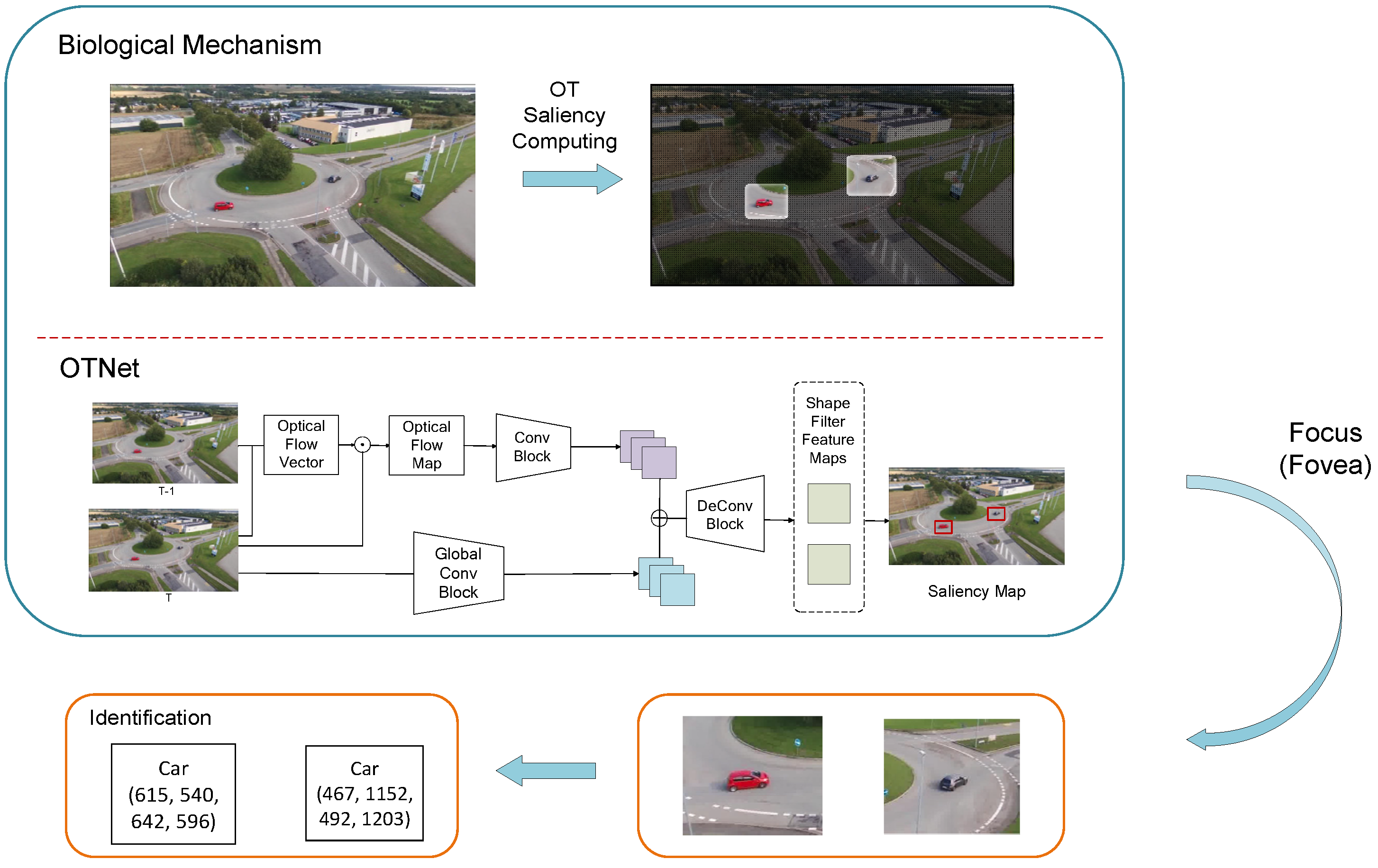
Animals have advantages when it comes to SOD, especially birds. Birds have the capability to locate small objects, such as fish or rabbits, and even insects, from a complex background at a high altitude. These abilities benefit from their advanced vision system. Avian visual systems are highly developed and highly differentiated [27]. For a complex biological system, such as a bird, object detection is a three-stage process, comprising location, focus and identification. In this process, “location” and “identification” are the two computing stages, and “focus” is the action stage [28]. Our model is inspired mainly by the “location” stage, where the biological system computes spatial saliency and selects a potential area exclusively and efficiently. The optic tectum (OT) is the key nucleus that integrates and selects the visual stimulus saliency, which performs as the main spatial saliency processing unit and object location unit in the visual system [29]. Additionally, some of the OT neurons have different responses for different object sizes [30]. Therefore, it can act as a size filter for potential targets at the same time. In the midbrain network, OT has the strongest response of the small objects with saliency. This is the reason why we choose to seek inspiration with this part in the visual system. The structure of OT is shown in Figure 1.
Visual saliency, according to Itti [32], “is the distinct subjective perceptual quality which makes some items in the world stand out from their neighbors and immediately grab our attention”. The thing worth mentioning is that visual saliency arises from low-level and stereotypical computations in the early stage of visual processing. Therefore, the factors contributing to saliency are quite comparable between observers. This means that visual saliency, despite its subjective nature, still has a certain level of objectivity. From the biological standpoint, visual saliency is the certain information captured and filtered by the biological visual system in order to stimulate the system to complete the object detection process. The forms of saliency can be described as motion, pop-out and memory [32]. Motion refers to the relative movement of the object. Pop-out refers to the feature value that occurs rarely across space, such as different colors and textures. As for memory, since memory always involves higher level neural activity, we simplify the memory feature to be a template-matching process.
Based on the OT selectivity of the stimulus, we propose a bio-inspired anchor-free SOD algorithm that combines optical flow map, spatial saliency map and memory module. The three components refer to three mentioned forms of saliency, respectively. Our algorithm provides a novel solution to the challenging problem of SOD as well as a bridge connecting the avian vision system and computer vision system. Instead of artificially increasing the sample amount of the small objects like most other solutions, our model tries to raise the relative size of the small objects by locating them first. The experiments show that our algorithm is able to complete the SOD task with a satisfied result and has bio-interpretability at the same time.
2. Materials and Methods
Objectively, a small scale alone is not a necessary feature to trigger the saliency response. As discussed before, certain information must be captured and processed to make the object easier to detect. Therefore, we bring out this theory:
When OT is facing SOD tasks, it integrates some other feature dimensions with the small object to make the object salient, as this equation shows:
The stands for the integration process of the features. The , as previously mentioned, are features that contribute to visual saliency, including motion, pop-out and memory.
Our model integrates the saliency computing mechanism of OT and artificial neural network methods to complete the SOD tasks. The structure of the model is shown in Figure 2. The model contains three modules, and each module represents the computing process of a feature dimension. The temporal–spatial feature extraction module extracts and processes the motion feature of the object. The spatial feature extraction module mainly focusses on the pop-out feature. For the memory, as we mentioned before, the template-matching process is covered by a memory-based template-matching strategy. Other than the three modules, we also designed a novel loss function and the training strategy to maximize the performance of our model. A detailed description of the model is presented in the subsections below.
2.1. Temporal–Spatial Feature Extraction (Motion Module)
To capture the motion information of the object, we adopted the optical flow method in this module. Optical flow is used to describe the motion attributes of the feature points on the images. When a biological visual system observes a moving object, the object’s image forms a series of continuous frames on the retina. This continuous changing information constantly “flows” through the retina, just like a “flow” of light. Therefore, it is called optical flow.
To calculate the optical flow, we need to find the relation between the current and previous frames based on the temporal changes of the pixels in the image sequence and the correlation of the consecutive frames. With this relation, we can calculate the motion information of the objects in consecutive frames. In our case, the objects are sparse and the objects between the current and previous frames have a certain level of spatial consistency and brightness invariance. Therefore, we have a choice between the Lucas–Kanade optical flow method [33] (LK below) and the Kanade–Lucas–Tomasi tracking method [34] (KLT below).
The LK as the following assumptions:
- Grayscale invariance assumption: For a point in the real world, its grayscale is invariant on the pixel level.
- Perturbation invariance assumption: Any temporal-level perturbation will not cause drastic changes in the pixel level.
- Spatial consistency assumption: Adjacent points on the same surface will have similar motion, and this rule applies to the points at the pixel level as well.
Based on the first two assumptions, we have the following constraint equation as Equation (1):
means at moment , the grayscale of point .
Apply first-order Taylor expansion to the constraint equation, and we can obtain
R is the higher-level remainder and can be considered 0 in this case.
Therefore, it is easy to obtain
Divide by for both sides, and we obtain
As we can see, and are both the derivatives of distance with respect to time. By definition, and are the speed of the pixel point alone in the directions of x and y, respectively. Therefore, we can simplify the equation to
Convert the equation to the matrix form,
Based on the third assumption, we can assume that in a window, the optical flow value is a consistent value, that is
The KLT method is composed of two steps:
- A so-called GoodFeaturesToTrack (GFT) feature detection step. It detects features at positions in the image with edge-like or texture-rich structures.
- Apply the LK method for these detected feature points.
The idea behind KLT is that the LK accuracy is in theory better at edge-like locations in the image sequence. Therefore, with the GFT, it is more likely to obtain accurate feature tracks and is able to reduce the number of features to process in advance. We performed experiments on both methods and chose to adopt KLT due to the better performance.
Then we applied the least square method to obtain the optical flow vector. Multiplying the optical flow vector and the original image, we obtained the final optical flow map. This step adds spatial information to the calculated temporal information. In the next step, we used convolution and maxpooling to process the temporal–spatial map to the same size as the spatial feature map.
2.2. Spatial Feature Extraction (Network) (Pop-Out Module)
The “pop-out”, as the other important form of visual saliency, is more about spatial features instead of temporal features. In order to properly extract and process the spatial feature, we chose to adopt artificial neural network algorithms. As one of the most iconic deep learning methods, the convolutional neural network (CNN) has shown its strength in the image-processing area. The basic mechanisms of the CNN have the capability to extract and preserve the spatial features, especially for small objects. On the one hand, most “pop-out” spatial features, such as color, shape or orientation are easily extracted by the convolution process. On the other hand, the convolution process is more likely to preserve local features, while many other methods, such as visual transformer, focus more on the global features. This makes it more suitable for SOD tasks, where local features weigh much more than global features.
The deeper layers in the CNN contain more higher-level semantic information instead of spatial distribution information. The information it provides cannot directly contribute to the location task. Therefore, after merging the spatial and temporal features, we use three de-convolution blocks in our model. Each block consists of a convolution layer and a transpose convolution layer. These three blocks restore the feature map to 1/4 of the original image. The main goal of this process is to restore the spatial information as well as the distribution information of the objects. The network then marks the objects with calculated spatial saliency on the feature map in order to predict the location of the targets. The thing worth mentioning is that we chose to use a pre-trained model to finetune our dataset in order to lower the training difficulties of the network.
The backbone we used for this module is Resnet50 [35]. At the same time, to make a lite version of the backbnone, we simplified the Resnet50 by removing the last two of the four layers. Correspondingly, the last de-convolution block was also removed in order to keep the consistency of the size of the output feature map. We named the simplified backbone Resnet50-Lite and the model that adopted it, OTNet-Lite. By adopting a simplified backbone, we were able to reduce the trainable parameters by 15.31% and the floating-point operations per second (FLOPs) by 17.37%. Such a simplification led to different final performance in the experiments. The detailed results are shown in the Section 3.
2.3. Memory-Based Template Matching Strategy (Memory Module)
While animals hunt or avoid predators, they rely heavily on natural instinct and memory. As the model brought up by Lovett shows [36], a previous stimulus will continue to affect the later detection process. The bottom-up saliency information is modulated by the top-down information in birds’ memory during its object-detection process [37]. In this paper, we consider the modulation of the memory information as a template-matching process. At the same time, there are neurons selective to object size in OT [30], that is to say, OT is able to pre-classify the object based on the different size of the objects at the earlier stage of the neural response, and different results may refer to a class of objects with a similar size. Since this process itself has very low computational complexity and fast responding time, it is able to lower the difficulties and the complexity of the whole identification tasks without adding any additional workload.
In this module, we divide the objects into two different classes by their average size: tiny and small. These two classes refer to the objects with , and , where stands for the proportion of the object in the image. For these two sizes, we designed the template with the object’s center point as the center and the radius of , where is the average length for the corresponding object categories. In this module, we take the feature map obtained in the previous module and map it into two heatmaps by a convolution operation, corresponding to the estimation of the two size categories. We assume that the heatmap, which the predicted object appears on, indicates the size of the predicted object. The thing worth noticing is that in order to improve the template matching accuracy as much as possible while ensuring a certain level of redundancy, all of the template size is larger than the average size of the corresponding category of the objects but not exceeding 1.3 times the average object size.
To make better use of the ground truth (GT) in the training phase, we obtained our idea from CornerNet [15]. For an input , the corresponding GT is . Since we have three different size categories, we set . We consider the GT point as a key point and calculate the relative position of the key point on the feature map . We then map all the key points to the heatmap using a Gaussian kernel.
When the same class Gaussian overlaps, we choose the element-wise maximum.
Since we are achieving fuzzy location and pre-classification in this step, with these two different size-classes, the standard deviation is the constant value corresponding to the template size .
In the inference stage, the Laplacian filter is applied to each feature map output by the model. For the points on the feature map, the Laplacian transformed values are
The above transformation can increase the contrast between the saliency areas and the neighbor so that we can find the saliency areas more easily. The points with higher values on the processed feature maps are selected as the candidates of the center points of the saliency areas, and such areas are finally determined after global non-maximum suppression (NMS). For OTNet-C, which is able to perform fuzzy classification, it is necessary to further compare the values on the two feature maps at the same location and select the one with higher values as the class of the corresponding saliency area.
2.4. Version Setup
Based on the above modules, we divided the OTNet into three versions: OTNet, OTNet-C and OTNet-Lite. The setups for the three versions are as follows:
- OTNet: Drop the memory module and all the objects are considered to be in the same size-class. These are our original thoughts of a location-focused object detection model.
- OTNet-C: Apply the memory module. This is our approach to further shrink the size of the output box and make the relative size of the tiny objects larger.
- OTNet-Lite: Based on OTNet_3, simplify the backbone and the transpose convolution layers. This is the lite version with less parameter count and less computational complexity.
The detailed structures of our models are shown in Figure 3.
2.5. Loss Function and Training Strategy
When completing the model, we faced two kinds of imbalances in the sample: positive and negative sample imbalance, and class imbalance. We tried to eliminate the influence of the imbalance as much as possible by designing the loss function and the training strategy.
For the imbalance of positive and negative samples, we were inspired by the loss function in CenterNet [16] and modified it to fit our tasks. While training the model, we calculate the pixel wise loss for every predicted result as
The positive samples are defined as the center of the ground truth, that is, a pixel will only be considered to be a positive sample if . However, in our case, the distribution of small objects in the bird view from a high altitude is sparse. In an image of 128 × 128, only 10 pixels can be considered positive samples at most. This will make it difficult for the model to obtain enough information about the positive samples.
Under our definition, points around the center of the ground truth can also be considered positive samples. Combining with modification to the focal loss [14], which uses Gaussian distribution to add location information to the negative samples near the ground truth, our loss function is able to make the model converge faster without loss in performance.
Class imbalance is a common issue for object-detection tasks. The class imbalance not only exists between the sparsely distributed target pixels with a smaller total amount and an enormous amount of background pixels, but also exists between the fewer smaller objects and more larger objects because of the difficulties of sampling and labeling. Therefore, when training our model, to avoid the information of the smaller objects lost in the training process, we first train the model using the loss function mentioned above for 10 epochs. After this stage, we add different weights to the two heatmap, which represent objects with different sizes and then continue the training. With this stage-wise training method, the model is able to learn the location information before learning the category information.
3. Experiments and Results
3.1. Dataset and Training Parameters
We chose to train and test our model on the AU-AIR dataset [38]. The dataset was shot by an unmanned drone. The whole dataset contains 32,823 labeled video frames, including 8 different scenes and 8 different categories of vehicles. On the premise of retaining the ratio of every object type, we then removed some of the scenes whose object size did not meet the requirements, namely the scenes which only contained larger objects.
After cleaning, the dataset had 17,908 video frames left, while the average size of the objects was 1% of the image size. For each scene, we divided the dataset at a ratio of 9 to 1 as the training set and the test set, while maintaining consecutive frames. By this process, we retained the features of the original dataset to some extent. The amount and the average size of object types are shown in Table 1.
The dataset we chose contains 8 video clips, such as crossroads, parking lots and a small number of highway scenes, from multiple orientations, heights and angles. For each scene, we randomly selected 50–100 consecutive frames as the test set and the rest as the training set. In these images, we faced challenges, such as extremely small objects, occlusions, and viewpoint transitions, due to the different flight heights and angles. Moreover, the videos cover various lighting conditions due to the time of the day and the weather conditions (e.g., sunny, partly sunny, and cloudy) [36]. This also bring the challenge of objects with different colors and contrasts.
We padded the frames and resized them into 512 × 512 pixels as the model input. All of the data are free from additional augmentation. We set the batch size to be 32 and used Adam as an optimizer. The initial learning rate was set to be 1 × 10⁻⁴ and dropped to 90% for the next epoch. We trained our model on one NVDIA GeForce RTX 3090.
Something worth mentioning is that Resnet50 and Resnet50-Lite in our model are initialized with a dataset finetuned by pre-trained ImageNet. At the same time, for our 2-stage training method, after training using our loss function for 10 epochs, we used the ratio of [1, 0.3] to add weight to the positive samples in the two heatmaps and then continued to train the model for another 10 epochs. The weight ratio was determined based on the distribution of the object classes among the dataset in order to avoid the influence of the class imbalance. The lower the number of objects in a class, the higher the weight assigned for this class.
3.2. Metrics
In our experiments, we used recall, precision, average location precision, F1 score and mean average precision (mAP) to evaluate our model. Before viewing the result, we need to clarify the definitions of the metrics.
- IoU: The full name of IoU is intersection over union, which is a concept widely used in object-detection tasks. IoU calculates the overlap rate of the “prediction box” and “ground truth box”, that is, the ratio of their intersection and union. We did not directly use IoU as one of the metrics. However, the IoU value helps us to determine whether the results can be considered positive or negative. Details are shown in the next bullet point.
- Recall, precision, average location precision and F1 score: For the output patches of the model, we define the true positive (tp) as the predicted result, which has the IoU to the ground truth larger than the threshold , false positive (fp) to be the result which has IoU less than , and false negative (fn) to be the ground truth, which is not predicted. Therefore, we can have the recall rate asand the precision asSince we have the location result on three heatmaps corresponding to different object sizes, we calculated the average precision for every heatmap and defined it as the average location precision in order to further evaluate the model’s classification ability.F1 score, also called the balanced F score, is defined as the harmonic mean of the precision and recall rate:
- Mean average precision (mAP): The mAP was first brought up by the PASCAL visual Object Classes challenge. It is one of the most commonly used and accepted metrics in the field of object detection. The calculation of the mAP is based on the precision and recall rate. However, while the precision and recall rates focus more on the model’s performance for single class, the mAP takes the average precision for all the classes and calculates the mean. The average precision (AP) is defined aswhere P stands for the precision rate, R stands for the recall rate and P is a function that takes R as a parameter. Geometrically, this means the area under the curve. However, in the actual practice, an additional step to smoothen the curve is necessary, that is
This means to take the largest precision rate P when the recall rate is larger than R.
3.3. Complexity and Location Performance Experiment
In this experiment, we mainly tested the complexity and location performance of our models. For the complexity, we examined the training difficulty and computation complexity of our models. For the location performance, the metrics we used are precision rate, recall rate, average location precision rate, F1 score and processed frames per second (FPS).
This is to better examine the effectiveness of our memory-based template-matching strategy at the same time. The test set we used was extracted from the AU-AIR dataset as mentioned above.
3.3.1. Training Difficulty
The changing of the precision and recall rate through the training process is shown in Figure 4.
As shown, all three versions of the OTNet only require relatively few epochs to achieve satisfying results with the highest precision rate reaching 85.73% and the highest recall rate reaching 97.95%. This indicates that the model is able to massively save the time cost of training.
The thing worth noticing during the training process is that OTNet-C has better location performance than OTNet. This may be due to the fact that it takes time for the network to learn the features of all the objects when all the objects are considered as one category. However, in OTNet-C, due to the addition of the memory module, features are more concentrated among the same category objects, and learning them is easier. This proves the effectiveness of the memory module.
3.3.2. Computation Complexity
We measured the computation complexity of our models by counting the amount of total parameters, trainable parameters, FLOPs and the parameter size.
For the sake of comparison, we chose two of the most commonly used and widely accepted object detection models, MaskRCNN [11], and the location module of FCOS [18] which also known as the anchor proposal network. We set the input image size to be 512 × 512 and counted the mentioned indices on those two models. The result is shown in Table 2.
Since we only use the ResNet as the feature extractor, we did not train it. Therefore, as the table shows, the trainable parameter is significantly less than the total parameters. On the contrary, OTNet and OTNet-C have less differences. This is due to the fact that the only difference between two versions is the output heatmap (1 × 128 × 128 and 2 × 128 × 128).
As we can see from the table, as a location module, all versions of OTNet have a smaller parameter amount and less complexity than the other model, especially OTNet-Lite. Compared to the other two versions, OTNet-Lite has 55.53% less trainable parameters, 17.37% less FLOPs and 6.32% less parameter size. This comparison shows that this model is capable of achieving satisfying results with low computation complexity. This indicates that our model can be easier to implement into a relatively simple system while keep a lower energy cost. This is also a key feature of the biological visual system that inspired our research. In addition, this also means that this model is able to work as plug-in module while minimizing the overall computation complexity increase.
3.3.3. Location Performance
We tested the LK and KLT algorithm and present the result below in Figure 5. We set the window size for LK to be 30 × 30 for a 1920 × 1080 image. To make the results more intuitive and to ensure the integrity of the object, we multiplied the optic flow vector with the original image and displayed the regions with motions in the form of a bounding box.
As we can see from the figure above, or the same image with the same experimental setup, the basic LK algorithm misclassifies most of the regions as motion regions. This is mainly due to the fact that basic LK is computed window-by-window in the whole image, and the points within each window are treated as potential motion points, while KLT is only computed in the representative points in the image, thus reducing the misclassification.
We took a step further and compared the localization effects of these two algorithms in the whole model, using the same experimental setup. The result is shown in Table 3.
From the above table and figure, we can see that the optical flow map does not provide the model with enough location information of moving objects due to too many interference regions, resulting in its precision and recall being inferior to KLT, especially the high recall gap which indicates that when we use LK as the optical flow module of OTNet, OTNet cannot identify all targets from the complex environment.
Since there are very few brain-like location specific algorithms, we selected the brain-like saliency model constructed by Itti [39] based on human attention during visual search and the regional stability and saliency model proposed by Luo et al. [40] based on local center-surround difference and the global rarity of human visual perception for comparison. We consider the output saliency map of these two models as the location information.
The thing worth mentioning is that neither Itti’s method nor Luo’s method contains temporal information. For the sake of fair comparison, we took the intersection of output local information and the optic-flow map generated by the LK algorithm as the final saliency map. We applied matlab’s regionprops function to segment the regions in the output saliency map and obtained the bonding boxes for every region. The precision and recall rate were obtained by comparing the bonding boxes and the GT. All the experiments were performed using the AU-AIR dataset. The location performance of all three versions and the mentioned two methods is shown in Table 4.
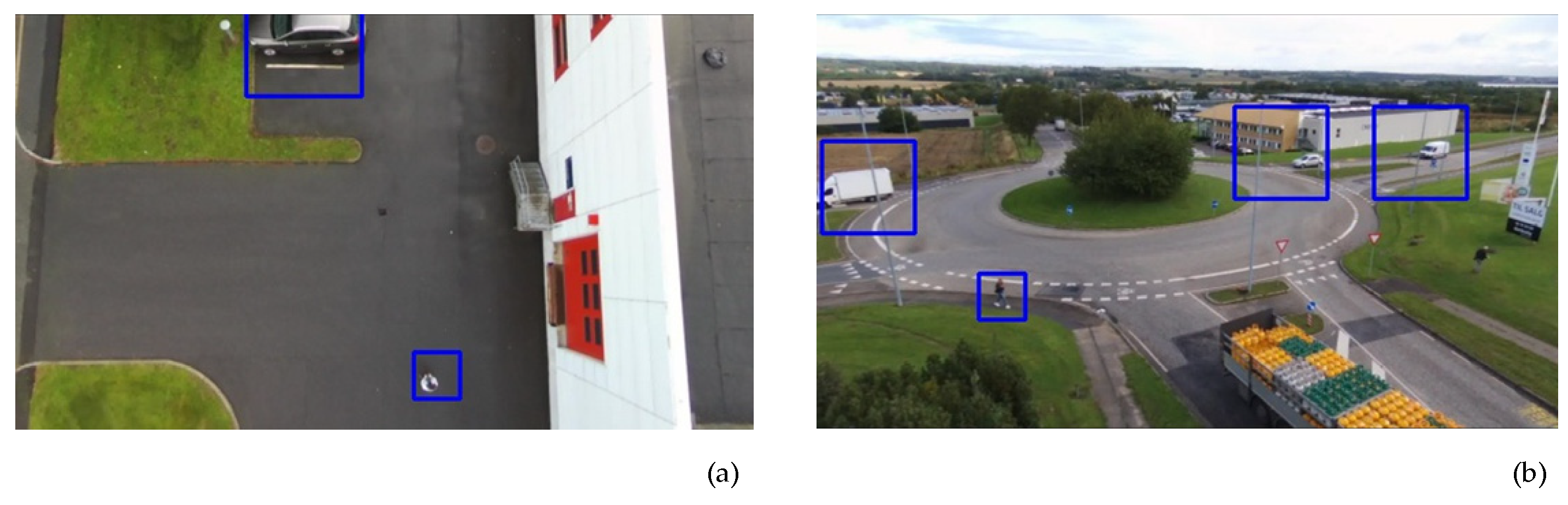
As the table shows, the overall location performance of all three models is very promising. At the same time, the much higher fps indicates that all of our models have much faster computing speed. The OTNet-C and OTNet-Lite have a higher recall rate due to the memory module. The thing worth mentioning that we limited the number of candidates for the object locations, which is similar to the anchors in the anchor-based model. Due to the sparsity of the small object distribution, we set that there are no more than 15 location candidates in each prediction map. Compared to the thousands of anchors, our model is much more efficient for the SOD tasks. Meanwhile, the high recall rate means that our model is able to locate most of the small objects with very few missing. Since our goal in this step is to provide enough candidates for the following detection model, such a high recall rate ensures we provide almost all the information needed by the next step. Some of the location result examples are shown in Figure 6.
The fps shows that the OTNet is able to process up to 33 frames with the size of 512 × 512 in 1 s. Such an impressive process speed is more than to provide real-time analysis to most of the video use case. The machine we run the model on is only regular tier work stations used for research purposes. There is room for improvement if the model is run on a better machine.
3.3.4. Average Location Precision
We also evaluate the effectiveness of our template-matching memory module. Since the OTNet does not contain a memory module, we performed the experiments on the other two versions of the model. We mainly evaluated the precision rate of the two size categories and the average location precision. The result is shown in Table 5.
The average precision shows that the strategy of dividing the objects into two categories is effective. Objects of different categories appear on different feature maps output by the model. As shown in Figure 7, the objects are marked differently using different box sizes. However, the number has room for improvement. The reason we are not able to achieve sufficiently satisfying results, especially with class 2 to which the smaller objects belong to, is that small objects lack feature information which makes them easier to confuse. In addition, the class imbalance and mislabeling of the data set are also the main reasons for this result.
3.4. Detection Performance Experiment
The main task of OTNet while facing the SOD tasks is to pre-locate the areas in which the small objects are most likely to appear. Therefore, in this section, we first conduct experiments to exam the performance improvement of the detection model brought by OTNet. We connected OTNet with yolov6s [41] as an external module. We first input the temporal image sequence into OTNet. OTNet finds the patches which are most likely to have the object. The output patches are then sent into yolov6s to perform object detection. We compared the performance of yolov6 with/without OTNet. The result is shown in Table 6.
After verifying the improvement that OTNet can bring to the detection model as an external module, we then chose some commonly accepted video object detection algorithms for comparison to examine the overall performance of our framework. FGFA [23] is an end-to-end learning framework for video detection, which leverages temporal coherence on feature level to improve accuracy. DFF [42] only applies the feature network on sparse key frames. The feature maps of a non-key frame are propagated from previous key frames, using feature flow. Temporal ROI Align [43] contains two new frameworks, MS ROI Align and temporal attentional feature aggregation (TAFA), compared with ROI Align to make the features of proposals contain temporal information. MEGA [24] integrates global and local feature information, and proposes a novel structure called long range memory module (LRM), which enables the current frame to obtain more comprehensive feature information. MAMBA [25] proposes a multi-level aggregation architecture via memory bank (MAMBA), and a generalized enhancement operation (GEO) to utilize knowledge from the whole video with reduced computational cost. The TransVOD [44] is the first end-to-end video object detection system based on spatial–temporal transformer architectures. Using temporal query encoder to fuse object queries and temporal deformable transformer decoder to obtain current frame detection results, it performs better than any other transformer-based model and Yolov6s, one the latest versions of the commonly accepted object detection model, yolo series. We used the OTNet with Yolov6s to compare with the above models.
We performed the experiments using the AU-AIR dataset. For the mentioned algorithms, we used resnet101 as the backbone and SGD as the optimizer. We set the learning rate to be 0.01, the momentum to be 0.9 and the weight decay rate to be 1 × 10⁻⁴. We stopped the training for the other models when the mAP on the validation set stopped rising and took the best mAP as the final results. The experiment results are shown in Table 7.
From Table 7, we can see that, comparing to other classic or state-of-the-art object detection methods, our OTNet has comparable results, especially better for smaller objects such as humans (39.32% better) and cars (40.01% better). For the objects motorbike and bicycles, most models are not able to detect them, including Yolov6s. With our model, the detection result for these two categories is significantly improved. Since our model is dedicated to smaller objects, the performance improvement on larger objects, such as truck, bus and trailer, is not as significant.
Another important fact that is worth mentioning is that, for a SOD task such as the dataset we chose, none of the above algorithms were able to perform as well as they did when detecting normal size objects. The reasons for such unsatisfying results are as follows:
- The size of the object is too small. From the tables, we can see that some categories such as the motorbike and the bicycle in the chosen dataset, are significantly smaller than others. Smaller objects mean fewer pixel points, which lead to less information contained in the image. This makes them much more difficult to detect than other categories and results in lower AP values.
- The class imbalance is another crucial reason. In the chosen dataset, motorbike, bicycle, bus and trailer have significantly smaller object amounts than other classes. This also leads to a lack of information when detecting the mentioned classes. As a result, the results for these classes are not as satisfying.
- The similar features of objects from different classes also add difficulty to the task. For instance, human, bicycle and motorbike share a fairly large amount of similar features, especially in the bird-view scenes. Combined with the lack of information caused by the above two reasons, the difficulty of the SOD detection tasks become much higher than normal tasks.
3.5. Ablation Experiment
In this section, we performed some ablation experiments in order to evaluate the effectiveness of our proposed modules. Since the performance of the memory module can be seen from the comparison between OTNet and OTNet-C, we mainly focused on evaluating the other two modules in this section. We designed a group of w/o experiments and chose precision, recall and F1 score as metrics to examine the effectiveness of the motion module and the pop-out module. The result is shown in Table 8.
It can be easily seen that both modules show their effectiveness in the experiments. Dropping the pop-out module causes a larger decrease than dropping the motion module, especially for the precision rate. Since the pop-out module is in charge for feature extraction, such a result is understandable. The thing worth noticing is that while dropping the motion module, the decrease in the recall rate is much more significant. This indicates that the model will miss some of the objects without this module.
4. Conclusions and Future Work
In this paper, facing the difficulties of the SOD tasks, inspired by the “location–focus–identification” process of the complex biological system, combining the mechanism of the OT and idea of visual saliency, we presented our bio-interpretable anchor-free SOD algorithm, OTNet. We designed three modules for the three forms of visual saliency: the optical-flow-based module for the “motion”, the feature-extraction-network-based module for the “pop-out”, and the template-matching module for “memory”. The experiment results show the efficiency of the modules as well as the whole algorithm. As the result shows, our algorithm has better performance when facing smaller objects. Not only does our algorithm have satisfying results, but it also shares another similar feature with the biological system: low computation cost. As the comparison between OTNet-Lite and other models shows, our algorithm is able to perform with significantly fewer trainable parameters and with faster computing speed. Importantly, we emphasize that the motivation of this work is not only to beat existing models in SOD, but to complement a method to provide bio-interpretability for detecting small objects, which we believe is a more important task. In practice, our method can also be deployed together with existing object detection models as a bio-interpretable plugin module to improve its performance.
For future work, it is important and valuable to further explore and understand the functions and mechanisms of the OT and the midbrain network. The inspiration we can obtain from the biological neural system is priceless and worth digging deeper. Another problem we faced during this study was finding high quality datasets that contain different categories of small objects. We have plans for further testing our model, and our own high-quality dataset is also on the way.
Author Contributions
Formal analysis, X.W.; Investigation, X.Z. and Y.C.; Methodology, P.H.; Software, P.H.; Supervision, L.S.; Writing–original draft, X.W. All authors have read and agreed to the published version of the manuscript.
Funding
This research received no external funding.
Acknowledgments
The authors are very grateful to the editors and reviewers for their valuable comments and suggestions.
Conflicts of Interest
The authors declare no conflict of interest.
References
- Rabbi, J.; Ray, N.; Schubert, M.; Chowdhury, S.; Chao, D. Small-Object Detection in Remote Sensing Images with End-to-End Edge-Enhanced GAN and Object Detector Network. Remote Sens. 2020, 12, 1432. [Google Scholar] [CrossRef]
- Wei, J.; He, J.; Zhou, Y.; Chen, K.; Tang, Z.; Xiong, Z. Enhanced Object Detection With Deep Convolutional Neural Networks for Advanced Driving Assistance. IEEE Trans. Intell. Transp. Syst. 2020, 21, 1572–1583. [Google Scholar] [CrossRef] [Green Version]
- Tong, K.; Wu, Y.; Zhou, F. Recent advances in small object detection based on deep learning: A review. Image Vis. Comput. 2020, 97, 103910. [Google Scholar] [CrossRef]
- Lin, T.-Y.; Maire, M.; Belongie, S.; Bourdev, L.; Girshick, R.; Hays, J.; Perona, P.; Ramanan, D.; Zitnick, C.L.; Dollár, P. Microsoft COCO: Common Objects in Context; Springer: Cham, Switzerland, 2015. [Google Scholar] [CrossRef]
- Dalal, N.; Triggs, B. Histograms of oriented gradients for human detection. In Proceedings of the 2005 IEEE Computer Society Conference on Computer Vision and Pattern Recognition (CVPR’05), San Diego, CA, USA, 20–26 June 2005; Volume 1, pp. 886–893. [Google Scholar]
- Lowe, D.G. Object recognition from local scale-invariant features. In Proceedings of the Seventh IEEE International Conference on Computer Vision, Kerkyra, Greece, 20–27 September 1999; Volume 2, pp. 1150–1157. [Google Scholar]
- Van de Sande, K.E.A.; Uijlings, J.R.R.; Gevers, T.; Smeulders, A.W.M. Segmentation as selective search for object recognition. In Proceedings of the 2011 International Conference on Computer Vision, Washington, DC, USA, 6–13 November 2011; pp. 1879–1886. [Google Scholar] [CrossRef]
- Girshick, R.; Donahue, J.; Darrell, T.; Malik, J. Rich Feature Hierarchies for Accurate Object Detection and Semantic Segmentation. In Proceedings of the IEEE Conference on Computer Vision and Pattern Recognition, Columbus, OH, USA, 23–28 June 2014; pp. 580–587. [Google Scholar]
- Girshick, R. Fast R-CNN. In Proceedings of the IEEE International Conference on Computer Vision, Santiago, Chile, 7–13 December 2015; pp. 1440–1448. [Google Scholar]
- Ren, S.; He, K.; Girshick, R.; Sun, J. Faster R-CNN: Towards Real-Time Object Detection with Region Proposal Networks. In Advances in Neural Information Processing Systems; IEEE Transactions on Pattern Analysis and Machine Intelligence: New York, NY, USA, 2015; Volume 39, pp. 1137–1149. [Google Scholar]
- He, K.; Gkioxari, G.; Dollar, P.; Girshick, R. Mask R-CNN. In Proceedings of the IEEE International Conference on Computer Vision, Venice, Italy, 22–29 October 2017; pp. 2961–2969. [Google Scholar]
- Redmon, J.; Divvala, S.; Girshick, R.; Farhadi, A. You Only Look Once: Unified, Real-Time Object Detection. In Proceedings of the IEEE Conference on Computer Vision and Pattern Recognition, Las Vegas, NV, USA, 27–30 June 2016; pp. 779–788. [Google Scholar]
- Liu, W.; Anguelov, D.; Erhan, D.; Szegedy, C.; Reed, S.; Fu, C.-Y.; Berg, A.C. SSD: Single Shot MultiBox Detector. In Computer Vision–ECCV 2016, Lecture Notes in Computer Science; Leibe, B., Matas, J., Sebe, N., Welling, M., Eds.; Springer International Publishing: Cham, Switzerland, 2016; pp. 21–37. [Google Scholar] [CrossRef] [Green Version]
- Lin, T.-Y.; Goyal, P.; Girshick, R.; He, K.; Dollar, P. Focal Loss for Dense Object Detection. In Proceedings of the IEEE International Conference on Computer Vision, Venice, Italy, 22–29 October 2017; pp. 2980–2988. [Google Scholar]
- Law, H.; Deng, J. CornerNet: Detecting Objects as Paired Keypoints. In Proceedings of the European Conference on Computer Vision (ECCV), Munich, Germany, 8–14 September 2018; pp. 734–750. [Google Scholar]
- Duan, K.; Bai, S.; Xie, L.; Qi, H.; Huang, Q.; Tian, Q. CenterNet: Keypoint Triplets for Object Detection. In Proceedings of the IEEE/CVF International Conference on Computer Vision, Seoul, Korea, 27 October–2 November 2019; pp. 6569–6578. [Google Scholar]
- Zhu, C.; He, Y.; Savvides, M. Feature Selective Anchor-Free Module for Single-Shot Object Detection. In Proceedings of the IEEE/CVF Conference on Computer Vision and Pattern Recognition, Long Beach, CA, USA, 15–20 June 2019; pp. 840–849. [Google Scholar]
- Tian, Z.; Shen, C.; Chen, H.; He, T. FCOS: Fully Convolutional One-Stage Object Detection. In Proceedings of the IEEE/CVF International Conference on Computer Vision, Seoul, Korea, 27 October–2 November 2019; pp. 9627–9636. [Google Scholar]
- Kong, T.; Sun, F.; Liu, H.; Jiang, Y.; Li, L.; Shi, J. FoveaBox: Beyound Anchor-Based Object Detection. IEEE Trans. Image Process. 2020, 29, 7389–7398. [Google Scholar] [CrossRef]
- Jiao, L.; Zhang, R.; Liu, F.; Yang, S.; Hou, B.; Li, L.; Tang, X. New Generation Deep Learning for Video Object Detection: A Survey. IEEE Trans. Neural Netw. Learn. Syst. 2022, 33, 3195–3215. [Google Scholar] [CrossRef] [PubMed]
- Kang, K.; Li, H.; Yan, J.; Zeng, X.; Yang, B.; Xiao, T.; Zhang, C.; Wang, Z.; Wang, R.; Wang, X.; et al. T-CNN: Tubelets With Convolutional Neural Networks for Object Detection From Videos. IEEE Trans. Circuits Syst. Video Technol. 2018, 28, 2896–2907. [Google Scholar] [CrossRef] [Green Version]
- Dosovitskiy, A.; Fischer, P.; Ilg, E.; Hausser, P.; Hazirbas, C.; Golkov, V.; van der Smagt, P.; Cremers, D.; Brox, T. FlowNet: Learning Optical Flow With Convolutional Networks. In Proceedings of the IEEE International Conference on Computer Vision, Santiago, Chile, 7–13 December 2015; pp. 2758–2766. [Google Scholar]
- Zhu, X.; Wang, Y.; Dai, J.; Yuan, L.; Wei, Y. Flow-Guided Feature Aggregation for Video Object Detection. In Proceedings of the IEEE International Conference on Computer Vision, Venice, Italy, 22–29 October 2017; pp. 408–417. [Google Scholar]
- Chen, Y.; Cao, Y.; Hu, H.; Wang, L. Memory Enhanced Global-Local Aggregation for Video Object Detection. In Proceedings of the 2020 IEEE/CVF Conference on Computer Vision and Pattern Recognition (CVPR), Seattle, WA, USA, 13–19 June 2020; pp. 10334–10343. [Google Scholar] [CrossRef]
- Sun, G.; Hua, Y.; Hu, G.; Robertson, N. MAMBA: Multi-level Aggregation via Memory Bank for Video Object Detection. In Proceedings of the AAAI Conference on Artificial Intelligence 35, Online, 2–9 February 2021; pp. 2620–2627. [Google Scholar] [CrossRef]
- Xiao, F.; Lee, Y.J. Video Object Detection with an Aligned Spatial-Temporal Memory. In Proceedings of the European Conference on Computer Vision (ECCV), Munich, Germany, 8–14 September 2018; pp. 485–501. [Google Scholar]
- Sridharan, D.; Schwarz, J.S.; Knudsen, E.I. Selective attention in birds. Curr. Biol. 2014, 24, R510–R513. [Google Scholar] [CrossRef] [PubMed] [Green Version]
- Zhaoping, L. From the optic tectum to the primary visual cortex: Migration through evolution of the saliency map for exogenous attentional guidance. Curr. Opin. Neurobiol. 2016, 40, 94–102. [Google Scholar] [CrossRef] [PubMed] [Green Version]
- Mysore, S.P.; Asadollahi, A.; Knudsen, E.I. Global Inhibition and Stimulus Competition in the Owl Optic Tectum. J. Neurosci. 2010, 30, 1727–1738. [Google Scholar] [CrossRef] [PubMed] [Green Version]
- Del Bene, F.; Wyart, C.; Robles, E.; Tran, A.; Looger, L.; Scott, E.K.; Isacoff, E.Y.; Baier, H. Filtering of Visual Information in the Tectum by an Identified Neural Circuit. Science 2010, 330, 669–673. [Google Scholar] [CrossRef] [PubMed] [Green Version]
- Asadollahi, A.; Knudsen, E.I. Spatially precise visual gain control mediated by a cholinergic circuit in the midbrain attention network. Nat. Commun. 2016, 7, 13472. [Google Scholar] [CrossRef] [PubMed] [Green Version]
- Itti, L. Visual salience. Scholarpedia 2007, 2, 3327. [Google Scholar] [CrossRef]
- Lucas, B.; Kanade, T. An Iterative Image RegistrationTechnique with an Application to Stereo Vision. In Proceedings of the 7th International Joint Conference on Artificial Intelligence (IJCAI), San Francisco, CA, USA, 24–28 August 1981; pp. 674–679. [Google Scholar]
- Tomasi, C.; Kanade, T. Detection and Tracking of Point Features; Carnegie Mellon University Technical Report CMU-CS-91-132; Carnegie Mellon University: Pittsburgh, PA, USA, 1991. [Google Scholar]
- He, K.; Zhang, X.; Ren, S.; Sun, J. Deep Residual Learning for Image Recognition. In Proceedings of the IEEE Conference on Computer Vision and Pattern Recognition, Las Vegas, NV, USA, 27–30 June 2016; pp. 770–778. [Google Scholar]
- Lovett, A.; Bridewell, W.; Bello, P. Selection, Engagement, & Enhancement: A Framework for Modeling Visual Attention. In Proceedings of the Annual Meeting of the Cognitive Science Society 43, Vienna, Austria, 26–29 July 2021; 2021. [Google Scholar]
- Knudsen, E.I.; Schwarz, J.S. The Optic Tectum: A Structure Evolved for Stimulus Selection; Evolution of Nervous Systems; Elsevier: Amsterdam, The Netherlands, 2017; pp. 387–408. [Google Scholar]
- Bozcan, I.; Kayacan, E. AU-AIR: A Multi-modal Unmanned Aerial Vehicle Dataset for Low Altitude Traffic Surveillance. In Proceedings of the 2020 IEEE International Conference on Robotics and Automation (ICRA), Paris, France, 31 May–31 August 2020; pp. 8504–8510. [Google Scholar]
- Itti, L.; Koch, C. Computational modelling of visual attention. Nat. Rev. Neurosci. 2001, 2, 194–203. [Google Scholar] [CrossRef] [PubMed] [Green Version]
- Lou, J.; Zhu, W.; Wang, H.; Ren, M. Small target detection combining regional stability and saliency in a color image. Multimed. Tools Appl. 2017, 76, 14781–14798. [Google Scholar] [CrossRef]
- Li, C.; Li, L.; Jiang, H.; Weng, K.; Geng, Y.; Li, L.; Ke, Z.; Li, Q.; Cheng, M.; Nie, W.; et al. YOLOv6: A Single-Stage Object Detection Framework for Industrial Applications. arXiv 2022, arXiv:2209.02976. [Google Scholar] [CrossRef]
- Hu, Y.; Chen, Y.; Li, X.; Feng, J. Dynamic Feature Fusion for Semantic Edge Detection. arXiv 2019, arXiv:1902.09104. [Google Scholar] [CrossRef]
- Gong, T.; Chen, K.; Wang, X.; Chu, Q.; Zhu, F.; Lin, D.; Yu, N.; Feng, H. Temporal ROI Align for Video Object Recognition. In Proceedings of the AAAI Conference on Artificial Intelligence 35, Online, 2–9 February 2021; pp. 1442–1450. [Google Scholar] [CrossRef]
- Zhou, Q.; Li, X.; He, L.; Yang, Y.; Cheng, G.; Tong, Y.; Ma, L.; Tao, D. TransVOD: End-to-end Video Object Detection with Spatial-Temporal Transformers. arXiv 2022, arXiv:2201.05047. [Google Scholar]
Figure 1.
The transverse section of midbrain showing the OT [31].
Figure 1.
The transverse section of midbrain showing the OT [31].

Figure 2.
The structure of our algorithm.

Figure 3.
The detailed structures of the models. (a) The overall structure of the model. (b) The difference between OTNet and OTNet-Lite.
Figure 3.
The detailed structures of the models. (a) The overall structure of the model. (b) The difference between OTNet and OTNet-Lite.

Figure 4.
The changing of the precision and recall rate through the training process. (a) The precision rate changing. (b) The recall rate changing.
Figure 4.
The changing of the precision and recall rate through the training process. (a) The precision rate changing. (b) The recall rate changing.

Figure 5.
The structure of our algorithm. (a) The ground truth. (b) The KLT result. (c) The LK result.
Figure 5.
The structure of our algorithm. (a) The ground truth. (b) The KLT result. (c) The LK result.

Figure 6.
The location result of OTNet in different scenes. (a) Multi-objects. (b) Truncation. (c) Bird view. (d) Tiny objects. (e) Occlusion. (f) Low contrast.
Figure 6.
The location result of OTNet in different scenes. (a) Multi-objects. (b) Truncation. (c) Bird view. (d) Tiny objects. (e) Occlusion. (f) Low contrast.

Figure 7.
The classification result of OTNet-C. The larger boxes and the smaller boxes represent different categories. (a) Result for the parking lot scene. (b) Result for the circular road scene.
Figure 7.
The classification result of OTNet-C. The larger boxes and the smaller boxes represent different categories. (a) Result for the parking lot scene. (b) Result for the circular road scene.


Table 1.
The amount and average size of every object type.
| Human | Car | Truck | Van | Motorbike | Bicycle | Bus | Trailer | |
|---|---|---|---|---|---|---|---|---|
| Amount | 3178 | 46341 | 5174 | 5056 | 77 | 321 | 294 | 1050 |
| Avg. size (%) | 0.4276 | 0.7248 | 2.1832 | 1.0874 | 0.3601 | 0.5390 | 2.3758 | 2.5178 |
Table 2.
The computation complexity results.
| Model | Total Params | Trainable Params | FLOPs | Params Size |
|---|---|---|---|---|
| OTNet | 30.01 M | 6.50 M | 27.17 | 114.48 MB |
| OTNet-C | 30.01 M | 6.50 M | 27.17 | 114.48 MB |
| OTNet-Lite | 28.45 M | 2.89 M | 22.45 | 107.24 MB |
| MaskRCNN [11] | 27.39 M | 27.37 M | 134.42 | 177.61 MB |
| FCOS [18] | 30.01 M | 29.78 M | 128.24 | 129.08 MB |
When calculating FLOPs, we set the input size to be 512 × 512.
Table 3.
The location performance results of the models.
| Model | Precision | Recall | F1 Score |
|---|---|---|---|
| OTNe with LK | 81.18 | 88.38 | 84.63 |
| OTNet with KLT | 85.73 | 92.06 | 88.78 |
Table 4.
The location performance results of the models.
| Model | Backbone | Precision | Recall | F1 Score | fps |
|---|---|---|---|---|---|
| OTNet | Resnet50 | 85.73 | 92.06 | 88.78 | 27 |
| OTNet-C | Resnet50 | 82.97 | 97.95 | 89.94 | 27 |
| OTNet-Lite | Resnet50-Lite | 80.66 | 97.93 | 88.46 | 33 |
| Itti-Saliency [39] | / | 6.02 | 89.07 | 11.28 | 1.05 |
| RSS [40] | / | 8.16 | 52.95 | 14.14 | 14.2 |
All the numbers are in percentage. We set the to be 0.5.
Table 5.
The classification results of the models.
| Model | Class 1 Precision | Class 2 Precision | Average Location Precision |
|---|---|---|---|
| OTNet-C | 74.63 | 43.31 | 58.97 |
| OTNet-Lite | 69.86 | 39.40 | 54.63 |
All the numbers are in percentage.
Table 6.
The performance of yolov6 with/without OTNet.
| mAP (IoU = 0.5) | mAP (IoU = 0.75) | |
|---|---|---|
| Yolov6s [41] | 24.71 | 7.90 |
| OTNet + Yolov6s | 31.34 | 7.54 |
Table 7.
Comparison results (average precision) to other object detection models.
| Model | Human | Car | Truck | Van | Motorbike | Bicycle | Bus | Trailer | mAP (IoU = 0.5) |
|---|---|---|---|---|---|---|---|---|---|
| FGFA [23] | 23.30 | 25.64 | 57.31 | 33.88 | 0.02 | 0.05 | 0.17 | 11.99 | 19.00 |
| DFF [42] | 17.78 | 22.53 | 46.19 | 27.22 | 0.00 | 0.03 | 0.11 | 9.98 | 15.50 |
| Temporal [43] | 20.39 | 27.72 | 59.54 | 37.91 | 0.03 | 0.06 | 0.46 | 9.98 | 19.80 |
| MEGA [24] | 18.53 | 29.57 | 49.05 | 32.98 | 0.78 | 0.00 | 0.30 | 5.22 | 17.05 |
| MAMBA [25] | 15.69 | 24.98 | 40.93 | 26.41 | 0.00 | 0.00 | 0.17 | 2.89 | 13.88 |
| TransVOD [44] | 23.93 | 36.58 | 58.61 | 41.73 | 1.68 | 0.01 | 0.35 | 8.82 | 21.50 |
| Yolov6s [41] | 30.44 | 41.89 | 60.43 | 48.52 | 0.00 | 0.50 | 0.79 | 15.22 | 24.72 |
| Ours | 42.41 | 58.65 | 47.13 | 51.36 | 0.87 | 32.07 | 0.54 | 17.73 | 31.34 |
All the numbers are in percentage.
Table 8.
The w/o experiments’ results.
| Precision | Recall | F1 Score | |
|---|---|---|---|
| OTNet | 85.73 | 92.06 | 88.78 |
| w/o Motion Module | 78.94 | 80.26 | 79.69 |
| w/o Pop-out Module | 33.15 | 74.10 | 45.79 |
All the numbers are in percentage.
Publisher’s Note: MDPI stays neutral with regard to jurisdictional claims in published maps and institutional affiliations. |
© 2022 by the authors. Licensee MDPI, Basel, Switzerland. This article is an open access article distributed under the terms and conditions of the Creative Commons Attribution (CC BY) license (https://creativecommons.org/licenses/by/4.0/).
Share and Cite
MDPI and ACS Style
Hu, P.; Wang, X.; Zhang, X.; Cang, Y.; Shi, L. OTNet: A Small Object Detection Algorithm for Video Inspired by Avian Visual System. Mathematics 2022, 10, 4125. https://0-doi-org.brum.beds.ac.uk/10.3390/math10214125
AMA Style
Hu P, Wang X, Zhang X, Cang Y, Shi L. OTNet: A Small Object Detection Algorithm for Video Inspired by Avian Visual System. Mathematics. 2022; 10(21):4125. https://0-doi-org.brum.beds.ac.uk/10.3390/math10214125
Chicago/Turabian StyleHu, Pingge, Xingtong Wang, Xiaoteng Zhang, Yueyang Cang, and Li Shi. 2022. "OTNet: A Small Object Detection Algorithm for Video Inspired by Avian Visual System" Mathematics 10, no. 21: 4125. https://0-doi-org.brum.beds.ac.uk/10.3390/math10214125
Note that from the first issue of 2016, this journal uses article numbers instead of page numbers. See further details here.