Probabilistic Interpretations of Fractional Operators and Fractional Behaviours: Extensions, Applications and Tribute to Prof. José Tenreiro Machado’s Ideas

Abstract

This paper extends and illustrates a probabilistic interpretation of the fractional derivative operator proposed by Pr. José Tenreiro Machado. While his interpretation concerned the probability of finding samples of the derivate signal in the expression of the fractional derivative, the present paper proposes interpretations for other fractional models and more generally fractional behaviours (without using a model). It also proposes probabilistic interpretations in terms of time constants and time delay distributions. It shows that these probabilistic interpretations in terms of time delay distributions can be connected to the physical behaviour of real systems governed by adsorption or diffusion phenomena.

1. Introduction

As part of this special issue in tribute to our colleague José Tenreiro Machado, this paper is an analysis of one of his works and serves as a basis for a deeper reflection on the origins of fractional behaviors and their modeling. The work by Professor José Tenreiro Machado analysed here is an interpretation of the fractional derivative operator [1].

Fractional operators remained abstract mathematical objects for a long time before applications in modelling [2] and control [3], but the latter did not give them a physical meaning. Finding interpretations and giving meaning, physical or not, to fractional operators has subsequently been the concern of many researchers. However, most of the interpretations proposed in the literature were not obtained from the observation of a given phenomenon but resulted from purely mathematical discussions [4,5,6,7,8,9]. In the case of non-commensurate fractional orders, certain interpretations even invalidated the model obtained [10]. But none of these approaches really help to understand the fractional behaviour observed in practice (fractional models and fractional behaviours are two distinct concepts), and they do not inform on the advantages and disadvantages of the fractional operators usually used to model these fractional behaviours (and we must not forget that other models exist [11,12,13]).

To try to obtain an interpretation which is the reflection of what occurs within a system having a fractional behaviour, one should not lose sight of the fact that these behaviours for the most part result from stochastic phenomena or result from geometries which are stochastic constructions (natural fractals). It is therefore interesting to seek an interpretation of these phenomena, and therefore of the fractional models very often used for their modelling, which is also stochastic in nature. A first attempt was made by Prof Tenreiro Machado in [1] with a probabilistic interpretation of the fractional differentiation operator based on the Grünwald-Letnikov definition of a derivative of fractional order.

In this paper, the idea of probabilistic interpretations for fractional models and behaviours is also used. Compared to [1], it proposes other types of interpretations and a confrontation of these interpretations with the physics of certain systems producing fractional behaviors. As defined in [11], we will say that a system has a fractional behaviours or more accurately a power law—like behaviour if its impulse response or if its frequency response exhibits a power law behaviour in a given time or frequency range, which can be evaluated from the system output autocorrelation function or system output power spectral density if the system input is a white noise. Note that fractional behaviours and fractional models are two distinct concepts. One designates a property of a physical system, the other designates a model class, among a set of model classes that capture fractional behaviours [13]. Thus, after recalling the results published in [1], this paper proposes a first probabilistic interpretation in terms of time constants distribution, resulting from the integral representation of fractional models’ impulse response. But this interpretation is only a macro representation of what happens in a system producing a fractional behaviour, and very often, it does not correspond to what happens internally, which is in most cases linked to the sequential movement of a multitude of agents in a constrained environment (the case of diffusion, aggregation and adsorption for example). Thus, another probabilistic interpretation in terms of time-delay distribution is proposed. As shown by this paper, this interpretation describes quite well what happens internally for adsorption or diffusion phenomena. For adsorption, this delay distribution it the time needed for particles to find their places on the adsorbing surface. In the case of diffusion, it describes the time needed for particles to cross a material.

2. Professor Tenreiro Machado’s Probabilistic Interpretation of the Fractional Derivative Operator

In [1], our colleague José Tenreiro Machado proposed a probabilistic interpretation of fractional differentiation based on the Grünwald-Letnikov definition of a derivative of fractional order $\nu$ of a signal $x\left(t\right)$. This derivative is given by:

$$D^{\nu }\left[x\left(t\right)\right]=\underset{h\to 0}{\lim }\left[\frac{1}{h^{\nu }}{\displaystyle \sum _{k=0}^{\infty }}\gamma \left(\nu ,k\right)x\left(t-kh\right)\right]$$

(1)

with

$$\gamma \left(\nu ,k\right)={\left(-1\right)}^k\frac{\mathsf{\Gamma }\left(\nu +1\right)}{k!\mathsf{\Gamma }\left(\nu -k+1\right)}$$

(2)

where $\mathsf{\Gamma }$ is the gamma function and $h$ is the sampling interval.

According to Professor Tenreiro Machado, and from a probability theory point of view, in relation (1):

-

the “present”, namely the sample $x\left(0\right)$, is seen with probability one,

-

each sample of the past, namely the samples $x\left(-kh\right)$ with $k\in \left[1, \infty \right[$ is weighted with the probability $\gamma \left(\nu ,k\right)$ and the expression $-{\displaystyle \sum }_{k=0}^{\infty }\gamma \left(\nu ,k\right)x\left(t-kh\right)$ can be viewed as the expected value of the random variable $X$, $E\left(X\right)$, such that $P\left(X=x\left(kh\right)\right)=\left|\gamma \left(\nu ,k\right)\right|$, $k\in \left[1, \infty \right[$.

This probabilistic interpretation is based on time information (samples) of the derivative signal. This idea can be extended to other operators with fractional behaviours and to the spectral content of these operators as demonstrated in the following paragraph.

3. Probabilistic Interpretation Based on the Spectral Content of Operators with Fractional Behaviours

The other probabilistic interpretation proposed can be revealed from the impulse response of the fractional operators considered. It is assumed that $H\left(s\right)$ denotes the transfer function of these operators. Using inverse Laplace transform, the corresponding impulse response defined by:

$$h\left(t\right)={ℒ}^{-1}\left\{H\left(s\right)\right\}=\frac{1}{2j\pi }{{\displaystyle \int }}_{c-j\infty }^{c+j\infty }H\left(s\right)e^{st}ds.$$

(3)

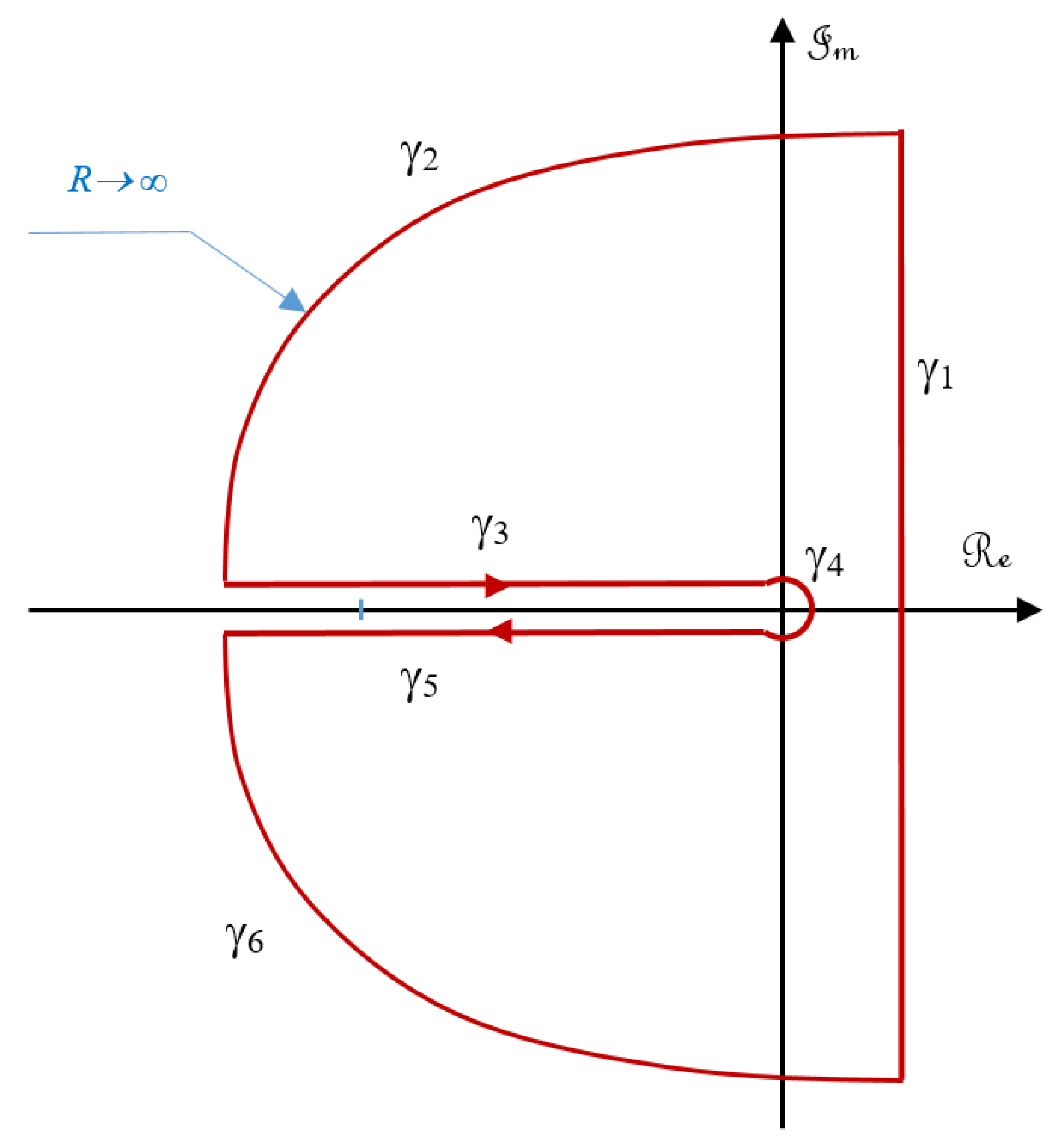
A Bromwich-Wagner path $\mathsf{\Gamma }$ is used to compute the integral in relation (3). The value of c is then taken greater than the abscissa of the singular point of $H\left(s\right)$. For instance, for the transfer function $H\left(s\right)=s^{-\nu }$, $\nu \in \left[0, 1\right]$, and for $t>0$, the considered path $\mathsf{\Gamma }$ is represented by Figure 1. As the function $s^{\nu }=0$ is not defined on ]−∞, 0], the path $\mathsf{\Gamma }$ avoid the negative axis and goes around the point $s=0$. It is shown by Figure 1.

Using the residue theorem, relation (3) can be rewritten as:

$$h\left(t\right)=-\frac{1}{2\pi j}{{\displaystyle \int }}_{\Gamma -{\gamma }_1}H\left(s\right)e^{ts}ds+{{\displaystyle \sum }}_{\begin{array}{c}poles\\ in \Gamma \end{array}}\mathrm{Res}\left[H\left(s\right)e^{ts}\right],$$

(4)

with, in the case of a simple pole $p$ for $H\left(s\right)e^{ts}$

$$Re{s}_p\left[H\left(s\right)e^{ts}\right]=\underset{\xi \to p}{\lim }\left(\xi -p\right)H\left(\xi \right)e^{t\xi }.$$

(5)

The computation of the poles of $H\left(s\right)$ is required by relation (4), relation that also shows that that the impulse (3) is made of two parts:

$$h\left(t\right)=h_p\left(t\right)+h_d\left(t\right).$$

(6)

The function $h_p\left(t\right)$ is computed from the poles of $H\left(s\right)$ (residues of the Cauchy method). The function $h_d\left(t\right)$ is defined by [14]:

$$h_d\left(t\right)={{\displaystyle \int }}_0^{\infty }\mu \left(z\right)e^{-tz}dz.$$

(7)

In relation (7), the function $\mu \left(x\right)$ is defined by [15]:

$$\mu \left(z\right)=\frac{1}{2i\pi }\left[H\left({\left(-z\right)}^{-}\right)-H\left({\left(-z\right)}^{+}\right)\right] \mathrm{with}\mu \left(z\right)\in ℝ.$$

(8)

Table 1. Table of impulse responses (inverse Laplace transforms) of some transfer functions with fractional behaviours.

${\mathit{H}}_{\mathit{i}}\left(\mathit{s}\right)$	${\mathit{h}}_{\mathit{i}}\left(\mathit{t}\right)$
$\frac{{{\displaystyle \sum }}_{l=0}^L{b}_l{s}^{{\beta }_l}}{{{\displaystyle \sum }}_{k=0}^K{a}_k{s}^{{\alpha }_k}}$	${\displaystyle \sum _{i=1}^r}{\displaystyle \sum _{j=1}^{n_i}}{r}_{ij}{Y}_j\left(t\right)e^{s_{i}t}+\frac{1}{\pi }{{\displaystyle \int }}_0^{+\infty }\frac{{{\displaystyle \sum }}_{k=0}^K{{\displaystyle \sum }}_{l=0}^L{a}_k{b}_l\sin \left(\left({\alpha }_k-{\beta }_l\right)\pi \right)x^{{\alpha }_k+{\beta }_l}}{{{\displaystyle \sum }}_{k=0}^K{a}_k^2{x}^{2{\alpha }_k}+{{\displaystyle \sum }}_{0\le k\le l\le K}{a}_k{a}_{l}cos\left(\left({\alpha }_k-{\alpha }_l\right)\pi \right)x^{{\alpha }_k+{\alpha }_l}}{e}^{-xt}dx$ From [15] with demonstration in [17]. $s_i$ are the poles.
$\frac{1}{s^{\nu }}$	$\frac{\sin \left(\nu \pi \right)}{\pi }\underset{0}{\overset{+\infty }{{\displaystyle \int }}}\frac{1}{x^{\nu }}{e}^{-xt}dx$
$\frac{1}{{\left(\frac{s}{{\omega }_l}+1\right)}^{\nu }}$	$\frac{\sin \left(\nu \pi \right)}{\pi }\underset{{\omega }_l}{\overset{+\infty }{{\displaystyle \int }}}\frac{{\omega }_l{}^{\nu }}{{\left(x-{\omega }_l\right)}^{\nu }}{e}^{-xt}dx$
$\frac{{\left(\frac{s}{{\omega }_h}+1\right)}^{\nu -1}}{{\left(\frac{s}{{\omega }_l}+1\right)}^{\nu }}$	$\frac{\sin \left(\nu \pi \right)}{\pi }\frac{{\omega }_l{}^{\nu }}{{\omega }_h{}^{\nu -1}}\underset{{\omega }_l}{\overset{{\omega }_h}{{\displaystyle \int }}}\frac{{\left({\omega }_h-x\right)}^{\nu -1}}{{\left(x-{\omega }_l\right)}^{\nu }}{e}^{-xt}dx$
$\frac{{\left(\frac{s}{{\omega }_h}+1\right)}^{\nu }}{{\left(\frac{s}{{\omega }_l}+1\right)}^{\nu }}$	${\left(\frac{{\omega }_l}{{\omega }_h}\right)}^{\nu }\left(\delta \left(t\right)+\frac{\sin \left(\nu \pi \right)}{\pi }\underset{{\omega }_b}{\overset{{\omega }_h}{{\displaystyle \int }}}\frac{{\left({\omega }_h-x\right)}^{\nu }}{{\left(x-{\omega }_l\right)}^{\nu }\left(s+x\right)}dx\right)$ $\delta \left(t\right)$: Dirac impulse
$\frac{1}{s}\frac{{\left(\frac{s}{{\omega }_l}+1\right)}^{1-\nu }}{{\left(\frac{s}{{\omega }_h}+1\right)}^{1-\nu }}$	${\left(\frac{{\omega }_h}{{\omega }_l}\right)}^{1-\nu } \left(H_e\left(t\right)+\frac{\sin \left(\left(1-\nu \right)\pi \right)}{\pi }\underset{{\omega }_l}{\overset{{\omega }_h}{{\displaystyle \int }}}\frac{{\left(x-{\omega }_l\right)}^{1-\nu }}{x{\left({\omega }_h-x\right)}^{1-\nu }}{e}^{-xt}dx\right)$ $H_e\left(t\right)$: Heaviside step function
$\frac{e^{-z\sqrt{as+b}}}{\sqrt{as+b}} a>0, b>0, z>0$	$\frac{1}{\pi }\underset{\raisebox{1ex}{$\mathrm{b}$}\!\left/ \!\raisebox{-1ex}{$a$}\right.}{\overset{+\infty }{{\displaystyle \int }}}\frac{\cos \left(z\sqrt{ax-b}\right)}{\sqrt{ax-b}}{e}^{-xt}dx$

provides several impulse responses of fractional transfer functions (with no pole and thus $h_p\left(t\right)=0$ for most) and computed using this method (demonstrations can be found in [16]).

The Laplace transform of function $h_d\left(t\right)$ is given by:

$$h_d\left(s\right)={{\displaystyle \int }}_0^{\infty }\frac{\mu \left(z\right)}{s+z}dz.$$

(9)

For a practical implementation, relation (9) must be truncated and discretized. But this implementation method is not very efficient. A large number of terms are needed in the sum resulting from the integral discretization. A solution consists in applying a change of variable to (9) before discretization [18]. Let $z=e^x$ and thus $dz=e^{x}dx$ this change of variable. Relation (9) becomes:

$$h_d\left(s\right)={{\displaystyle \int }}_{-\infty }^{\infty }\frac{\mu \left(e^x\right)}{\frac{s}{e^x}+1}dx.$$

(10)

Relation (10) can thus be viewed as the expectation of a random variable $X$, such that $P\left(X=\frac{1}{\raisebox{1ex}{$s$}\!\left/ \!\raisebox{-1ex}{$e^x$}\right.+1}\right)=\mu \left(e^x\right)$, $x\in ℝ$. Physically, if a real system is characterized by a fractional model such as those in Table 1 (or others), relation (10) implicitly provides information on the probability of encountering the time constant $\raisebox{1ex}{$1$}\!\left/ \!\raisebox{-1ex}{$e^x$}\right.$ in the model.

To illustrate this probabilistic interpretation, it is now proposed to use relation (10) to design a filter of the form

$$F_i\left(s\right)=\frac{1}{M}{\displaystyle \sum }_{k=1}^M\frac{1}{\frac{s}{e^x}+1}$$

(11)

in which the corner frequencies $e^{x_k}$ (or the time constant $\raisebox{1ex}{$1$}\!\left/ \!\raisebox{-1ex}{$e^{x_k}$}\right.$) are randomly selected with a probability density $\mu \left(e^x\right)$ where

$$\mu \left(e^x\right)=\frac{\sin \left(\nu \pi \right)}{\pi }\frac{\frac{e^{\nu x}}{a^{\nu }}}{1+2\frac{e^{\nu x}}{a^{\nu }}\cos \left(\nu \pi \right)+\frac{e^{2\nu x}}{a^{2\nu }}}$$

(12)

i.e., the function $\mu \left(e^x\right)$ involved in the impulse response of the transfer function (see line 1 of Table 1)

$$F_f\left(s\right)=\frac{1}{{\left(\frac{s}{a}\right)}^{\nu }+1}\hspace{1em}\hspace{1em}a>0\hspace{1em}\hspace{1em}0<\nu <1.$$

(13)

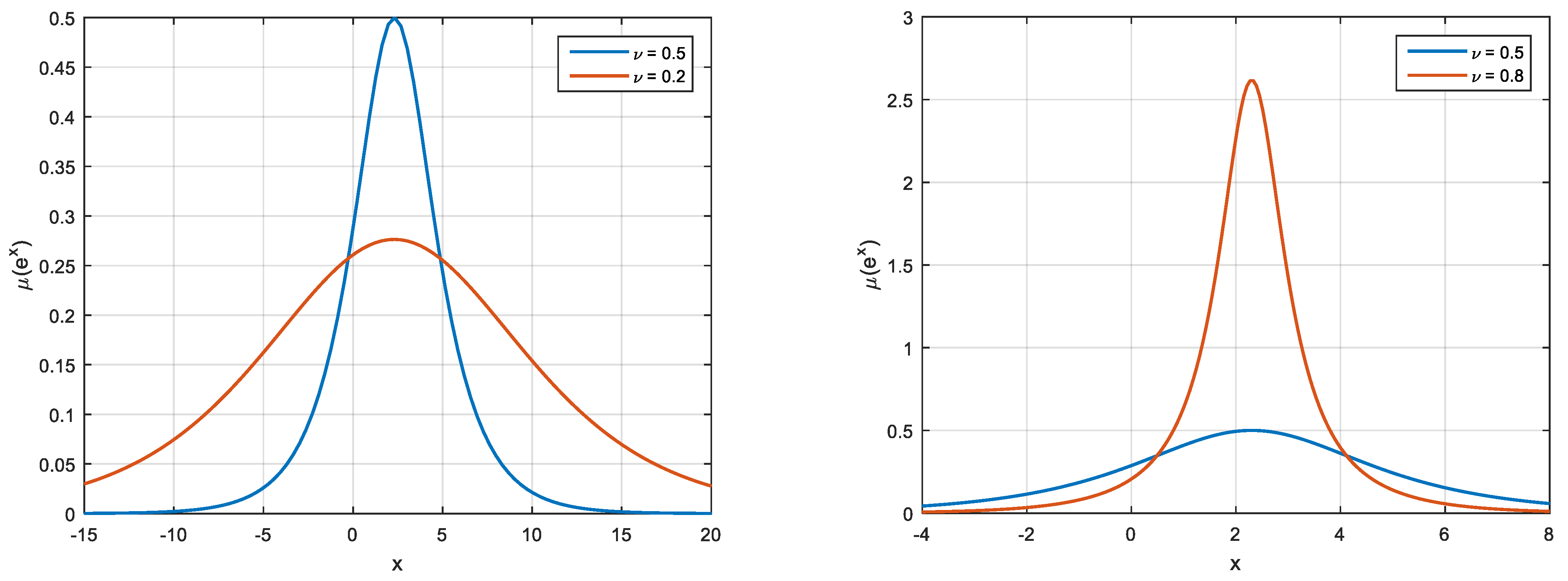
The function $\mu \left(e^x\right)$ given by relation (12) is represented by Figure 2 for various values of $\nu$ and $a=10$. It is interesting to note that all these curves resemble a normal law centred on the value $log\left(a\right)=log\left(10\right)\approx 2.3$.

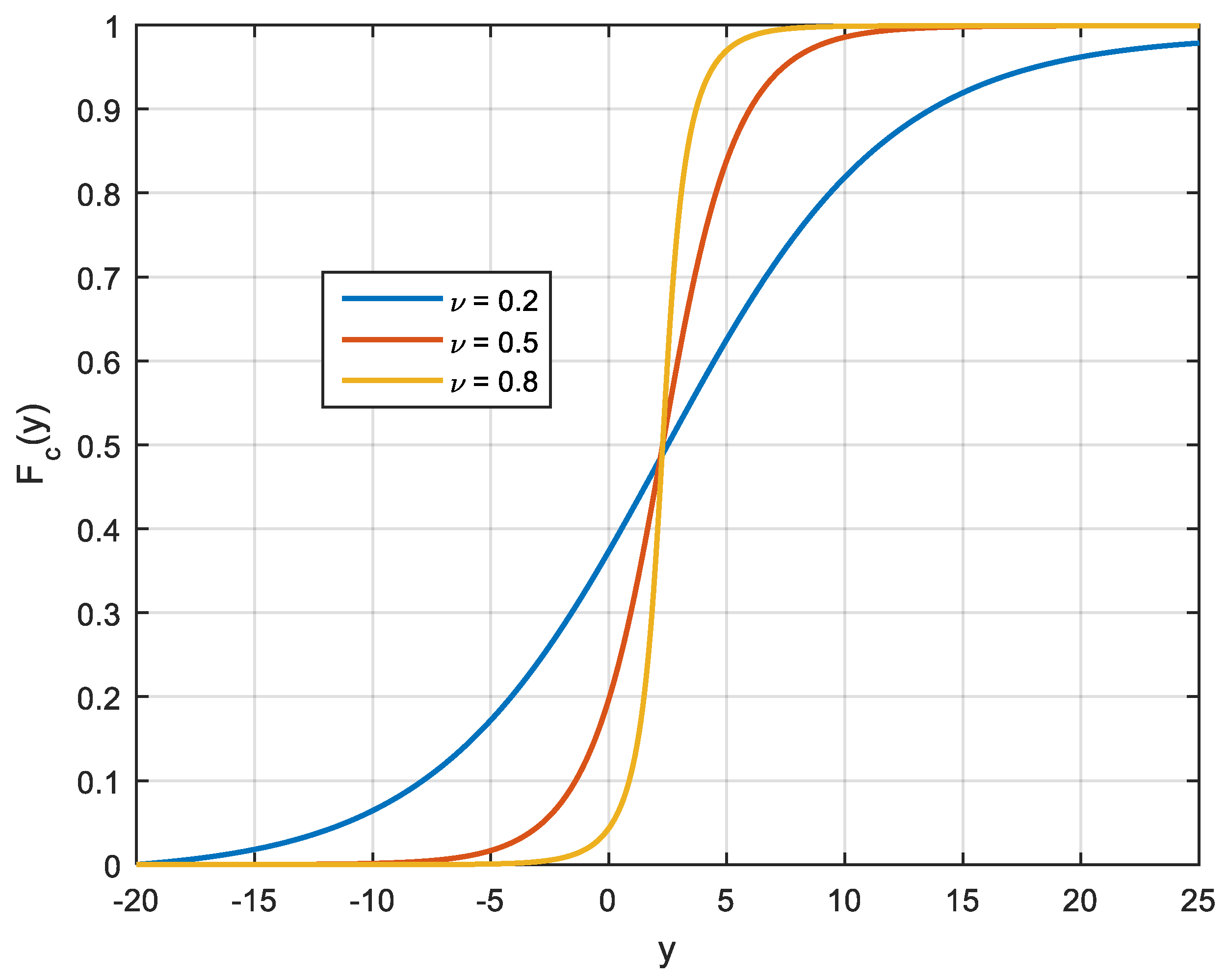
The cumulative distribution function

$$F_c\left(y\right)={{\displaystyle \int }}_{-\infty }^y\mu \left(e^x\right)dx$$

(14)

(evaluated numerically) is represented by Figure 3 for several values of $\nu$ and $a=10$.

To obtain the corner frequencies $e^{x_k}$ of relation (11), the following algorithm is used:

-

generate a random number $u_k$from the standard uniform distribution in the interval [0, 1];

-

compute$x_k=F_c^{-1}\left(u_k\right)$.

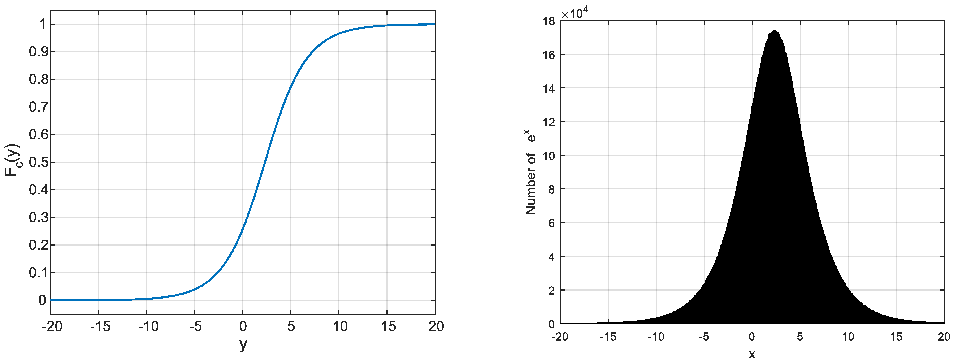
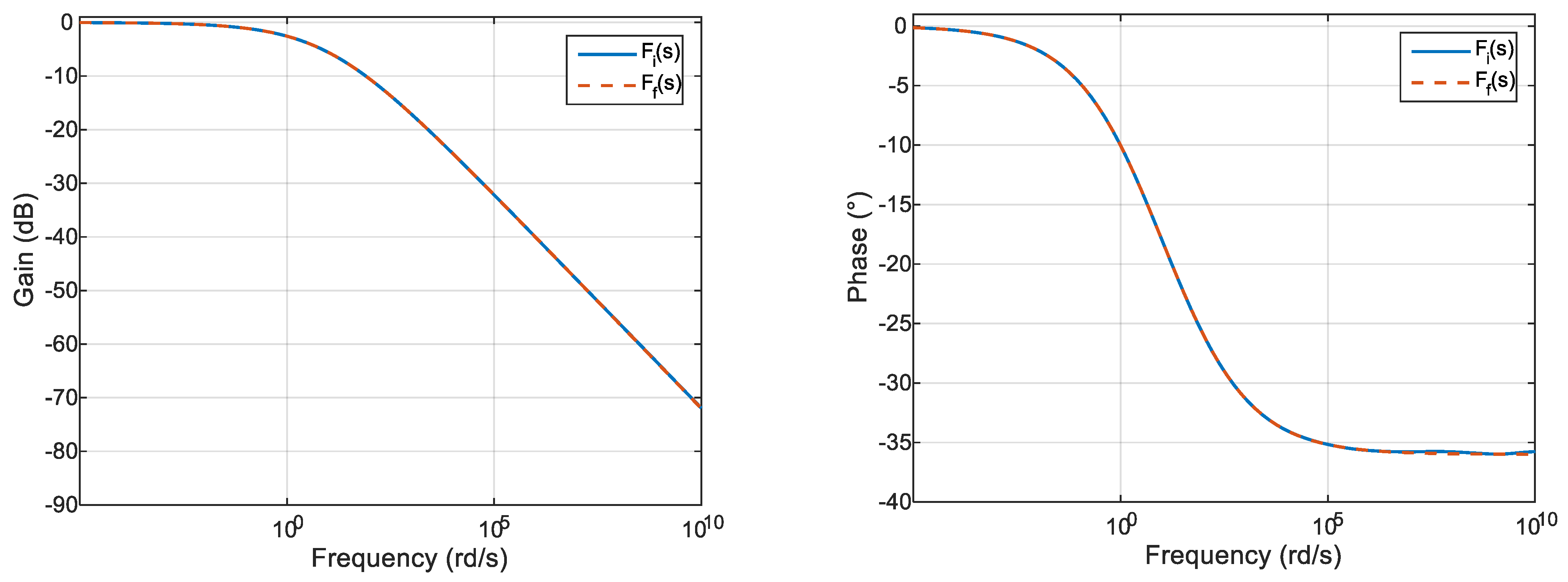
In the case of $\nu =0.4$ (in this case $h_p\left(t\right)=0$) and $a=10$, the cumulative distribution function provided by relation (14) and the histogram of $x_k$ generated by the algorithm above are represented by Figure 4. These figures are obtained after $50\times {10}^6$ random numbers $u_k$ have been generated. A comparison of the gain and phase diagrams of the transfer functions $F_i\left(s\right)$ and $F_f\left(s\right)$ is proposed in Figure 5. This comparaison validates the probabilistic interpretation done relating to time constants.

The probabilistic interpretation of fractional behaviors proposed in this section leads to the following remarks.

Modeling a real system by a fractional model amounts to considering that this system has a distribution of time constants (or corner frequencies) whose probability of occurrence is governed by the function $\mu \left(e^x\right)$.

This interpretation highlights that some fractional models, in particular those which, in the Laplace domain, involve fractional powers of the Laplace variable ($s^{\nu }$), induce the probability, admittedly low but not zero, of the presence in the model of infinitely large and infinitely small time constants, which is physically not realistic [19].

With a view to proposing more physically realistic models than the fractional models of the type mentioned above, it would be possible to work directly on a model having a substantially equal number of parameters and of the type

$$h_d\left(s\right)={{\displaystyle \int }}_{x_l}^{x_h}\frac{\mu \left(e^x\right)}{\frac{s}{e^x}+1}dx.$$

(15)

The characterization of a real physical phenomenon using such a model would then consist in identifying the probability density $\mu (.)$ after having described it by an appropriate function and the parameters $x_l$ and $x_h$. These two parameters can be fixed a priori from information on the sampling frequency of the measured signals and on the bandwidth (response time) of the physical phenomenon modeled. The author will describe this identification method in more detail in another paper.

This interpretation in terms of time constants distribution is interesting but does not necessarily reflect the physics of the modelled system. This is particularly the case of phenomena such as diffusion, adsorption, and aggregation, in which entities (atoms, molecules, people, etc.) evolve in a more or less constrained spatial domain.

In order to obtain a description that is even closer to the physical reality of systems with fractional behaviours, the following interpretation in terms of delays is proposed.

4. Probabilistic Interpretation Based on the Delay Approximation of Operators with Fractional Behaviours

The previous probabilistic interpretation based on time constants distribution does not well describe what happens in phenomena such as adsorption, which is now described.

4.1. Description of Adsorption Phenomena

Adsorption is the phenomenon which consists of the accumulation of a substance at the interface between two phases (gas-solid, gas-liquid, liquid-solid, liquid-liquid, solid-solid). It has its origin in the intermolecular forces of attraction, of varied nature and intensity, which are responsible for the cohesion of the condensed, liquid or solid phases [20,21]. Adsorption on solids is frequently used for the separation and purification of gases or the separation of solutes in liquids [22]. Adsorption is used in many industrial and academic applications [23,24] and in particular as water purification [22] and sensors [25,26].

Random Sequential Adsorption of RSA, is an idealized stochastic process often encountered in the literature to study chemical adsorption phenomenon. In the 1D case, it is first Flory [27] and Rényi [28] (car-parking problem) who studied RSA. The 2D case was also investigated in [29,30,31]. These latest studies focus on the final value of particles concentration and also on the kinetic behaviour of RSA.

To define RSA process, let consider a square plane substrate of edge length $L$ (thus leading to a surface $L^2$). Disk particles are supposed by this substrate and disk radius is supposed small in relation to substrate size $\left(R\ll L\right)$. During RSA process, particles fall sequentially onto the substrate. At each process iteration, the position of the fall is fixed randomly with a uniform distribution. A falling particle remains attached to the surface only if its surface covers a still free surface of the substrate, otherwise, the adsorption attempt fails. At the beginning of the process (time $t_0$), the substrate surface is supposed empty.

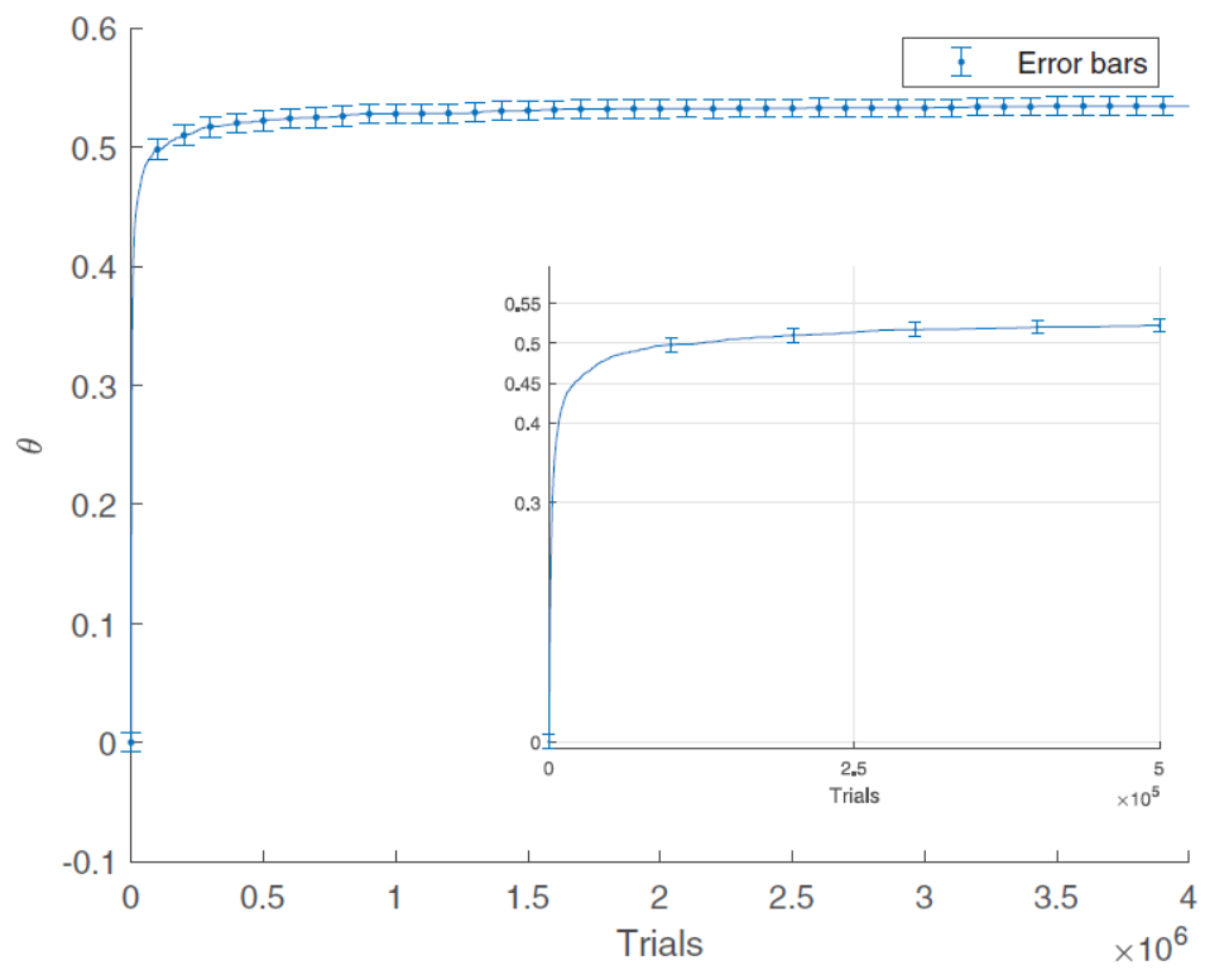
In the case $R=0.5$ and $L=100R$, the density $\theta \left(t\right)$ of the covered surface is shown in Figure 6 as a function of trials (number of discs that fell on the surface) which is denoted t in the sequel. The fluctuations of the value of $\theta \left(t\right)$ between several simulations are represented by error bars. These fluctuations result in the randomness of the process.

For high coverage regimes, it is suggested in the literature [31,32,33,34,35] that the covered surface can be described by a power law:

$${\theta }_{\infty }-\theta \left(t\right)~t^{1/2},$$

(16)

in which ${\theta }_{\infty }$ is the value of $\theta \left(t\right)$ when $t$ goes to infinity.

The RSA process and adsorption thus result in the stochastic behaviour of agents (atoms, molecules, people, etc.) in a constrained geometry, and the distribution of time constants struggles to explain the overall behaviour of all these agents. A time constant is indeed linked to a continuous time process whereas the placement of a disk in the RSA process is sequential.

4.2. Time Delay Distribution for Fitting Fractional Behaviours

José Tenreiro Machado’s probabilistic interpretation published in [1] was based on the sample distribution given in the Grünwald-Letnikov definition of a fractional derivative. But one can also see in this definition an interpretation which relates to a distribution of delay induced by the operator $s^{\nu }$ and which can be generalized to other fractional operators and behaviors. Indeed, Laplace transform applied to relation (1) leads to:

$$ℒ\left\{D^{\nu }\left[x\left(t\right)\right]\right\}=s^{\nu }x\left(s\right)=x\left(s\right)\underset{h\to 0}{\lim }\left[\frac{1}{h^{\nu }}{\displaystyle \sum }_{k=0}^{\infty }\gamma \left(\nu ,k\right)e^{-khs}\right]$$

(17)

and thus

$$s^{\nu }=\underset{h\to 0}{\lim }\left[\frac{1}{h^{\nu }}{\displaystyle \sum }_{k=0}^{\infty }\gamma \left(\nu ,k\right)e^{-khs}\right].$$

(18)

Using relation (17) and regarding the definition of the operator $s^{\nu }$, from a probability theory point of view it can be said that the delay operators $e^{-khs}$ with $k\in \left[1,\infty \right[$ are weighted with the probability $\gamma \left(\nu ,k\right)$ and the expression $-{{\displaystyle \sum }}_{k=0}^{\infty }\gamma \left(\nu ,k\right)e^{-khs}$ can be viewed as the expected value of the random variable $X$, $E\left(X\right)$, such that $P\left(X=e^{-khs}\right)=\left|\gamma \left(\nu ,k\right)\right|$, $k\in \left[1,\infty \right[$.

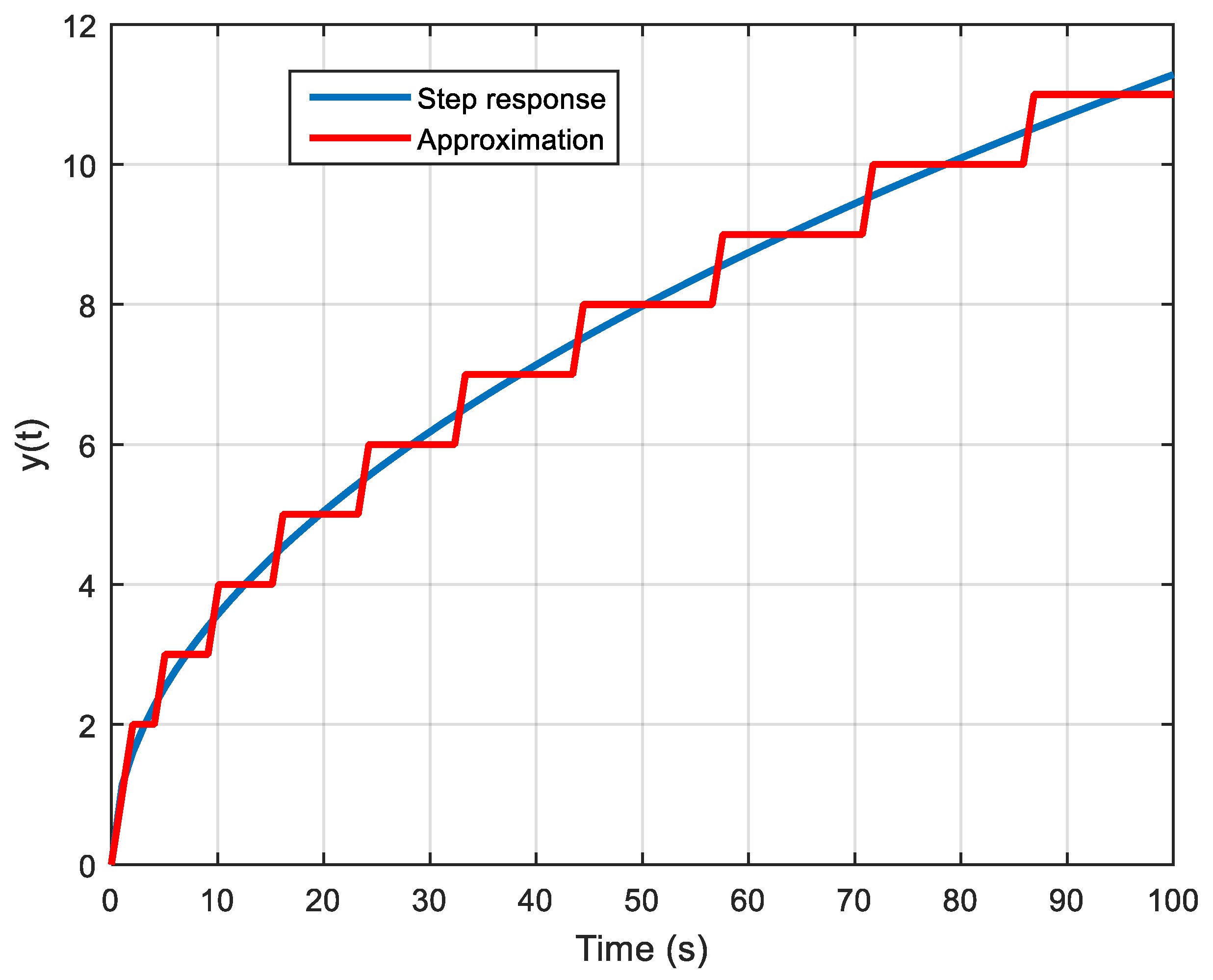
This idea can of course be extended to many other fractional operators. This is now highlighted graphically with the fractional integration operator $s^{-\nu }$. To explain how such a behaviour can be approximated by a delay distribution, the step response of the transfer function

$$H\left(s\right)=s^{-\nu } \mathrm{with} \nu =\frac{1}{2}$$

(19)

is analysed. It is defined by

$$y\left(t\right)=\frac{t^{1/2}}{\mathsf{\Gamma }\left(3/2\right)}$$

(20)

and is represented by Figure 7. This figure shows that this time response can be approximated by a distribution of delayed steps with the same magnitude $M$, thus permitting the following approximation in the Laplace domain:

$$Y\left(s\right)=ℒ\left\{y\left(t\right)\right\}\approx \frac{M}{s}{\displaystyle \sum }_{k=1}^N{e}^{-t_{k}s}$$

(21)

and thus

$$s^{-\nu }\approx M{{\displaystyle \sum }}_{k=0}^N{e}^{-t_{k}s} \mathrm{with} {\left(t_k\right)}^{1/2}=\mathsf{\Gamma }\left(3/2\right)kM.$$

(22)

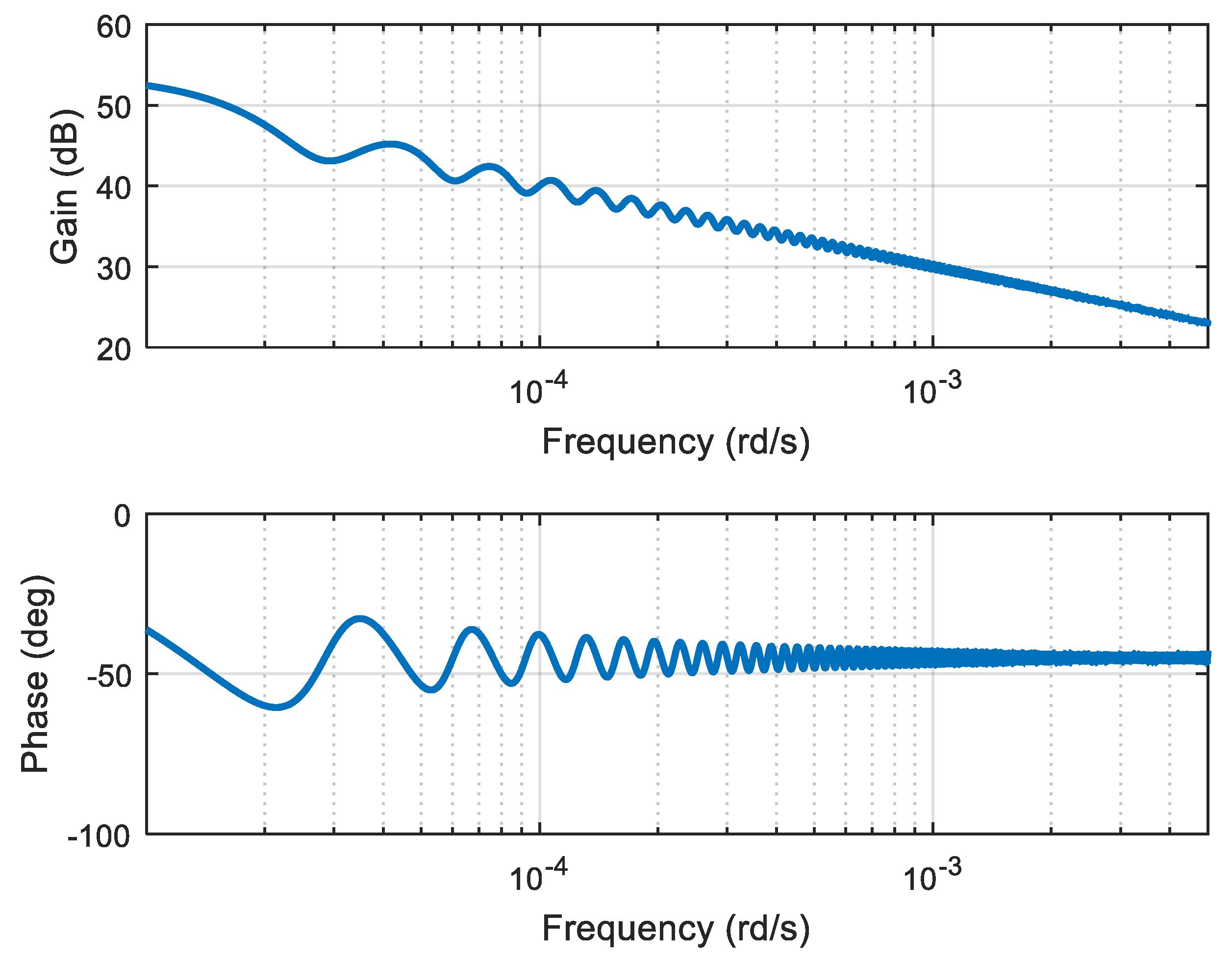
The frequency response of the approximation given by relation (21) is represented by Figure 8. This figure shows that the gain diagram decreases with a slope equal to $-20\nu$ dB per decade and a constant phase equal to $-90\nu$ degrees, like the frequency response of a fractional integrator.

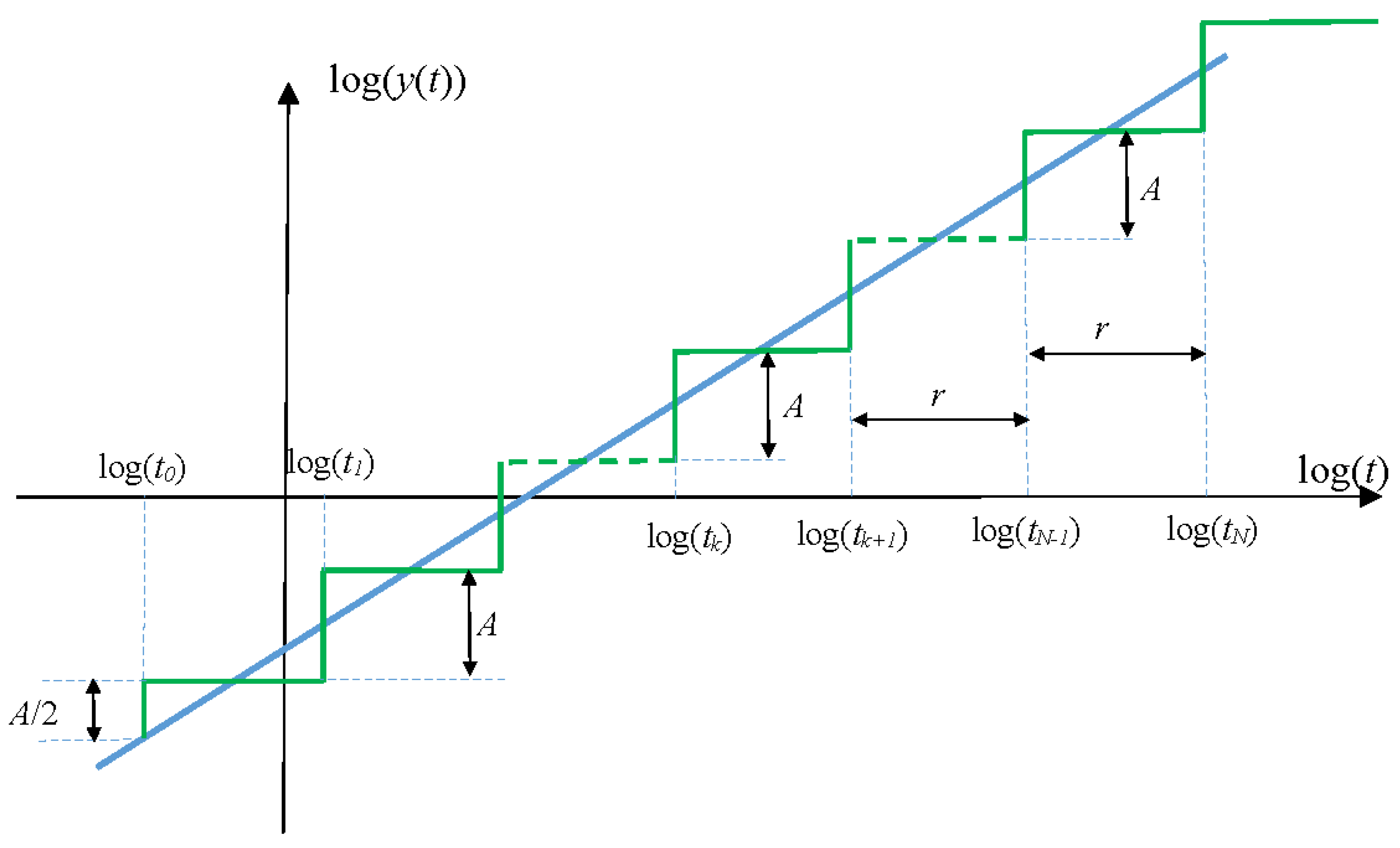
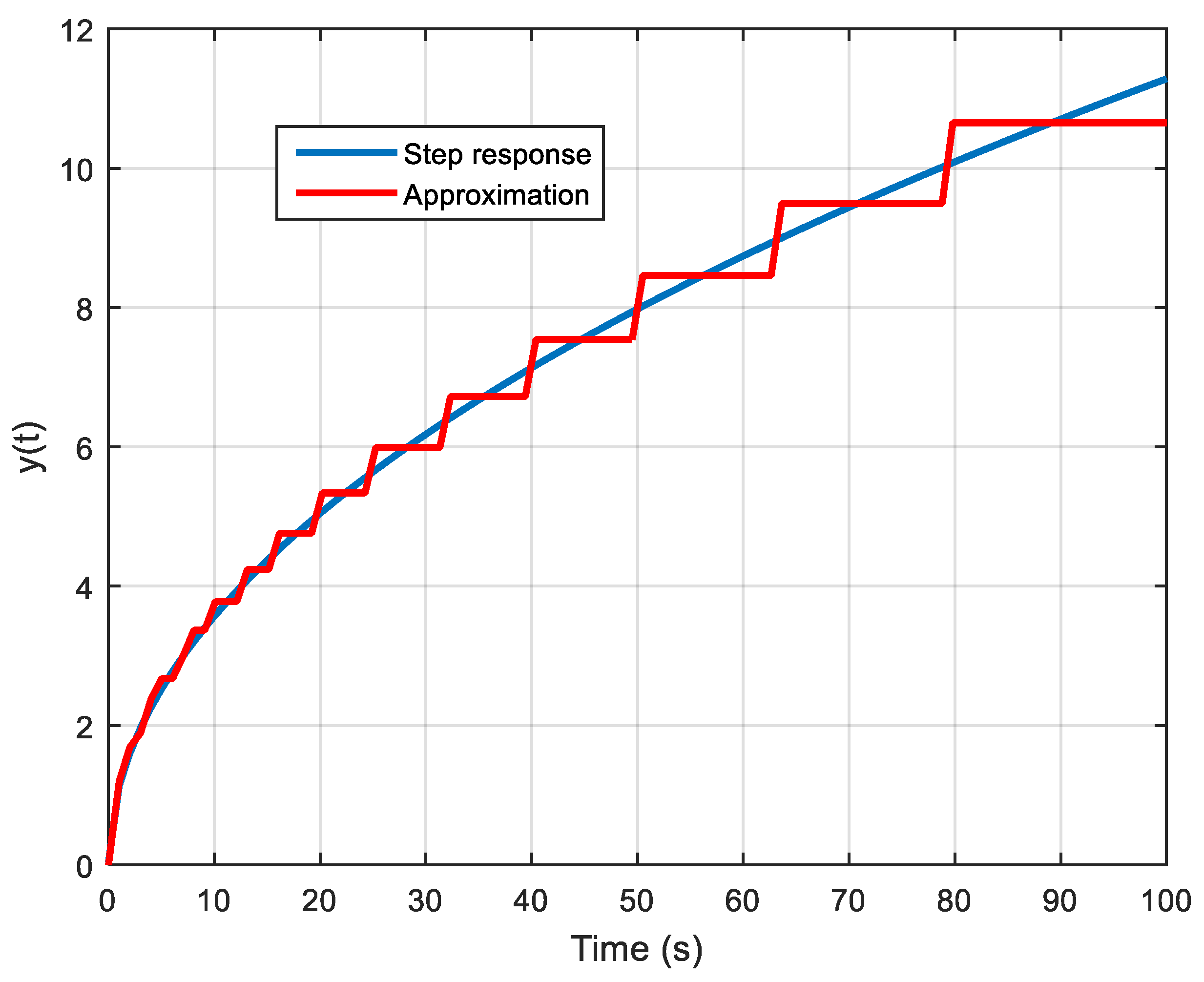
This approximation is of course not unique and an interesting one can be obtained by considering the logarithm of the fractional integrator step response as a function of the logarithm of time, namely a straight line whose slope is $\nu$. As shown by Figure 9, this straight line can be approximated by a distribution of steps of magnitude $A$ that occurs at time $t_k$ that are linked by the recurrence equation involving a constant factor $r$:

$$log\left(t_{k+1}\right)-log\left(t_k\right)=r \mathrm{and} \mathrm{thus} log\left(t_k\right)=log\left(t_0\right)+kr$$

(23)

or

$$t_k=t_0{e}^{kr}.$$

(24)

In such a situation, the fractional integrator step response admits in the Laplace domain the approximation

$$Y\left(s\right)=ℒ\left\{y\left(t\right)\right\}\approx \frac{1}{s}{\displaystyle \sum }_{k=0}^N{M}_k{e}^{-t_{k}s}$$

(25)

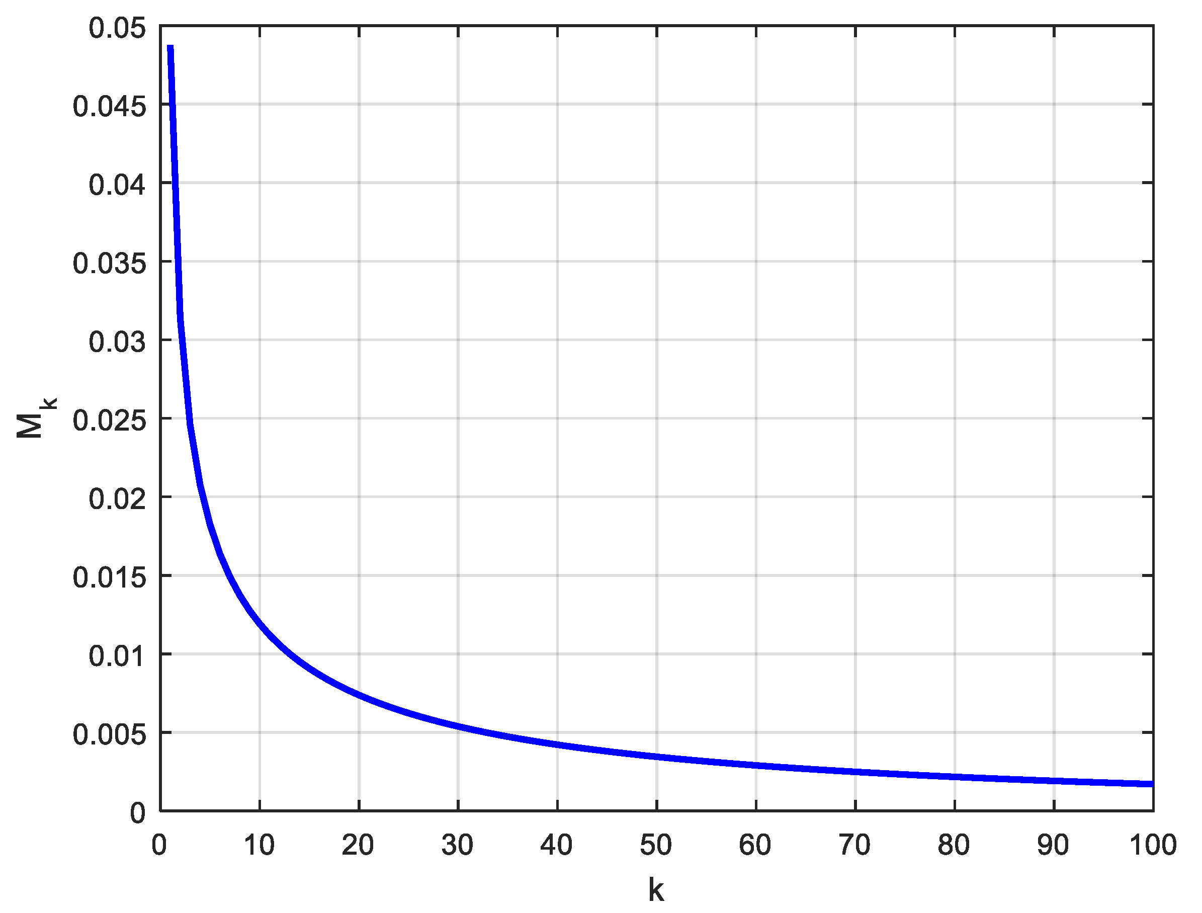
where the magnitudes $M_k$ are defined by:

$$M_0=\frac{1}{\mathsf{\Gamma }\left(3/2\right)}{t}_0^{\nu }{\left(\frac{t_1}{t_0}\right)}^{\nu /2}$$

(26)

$$M_k=M_{k-1}{\left(\frac{t_k}{t_{k-1}}\right)}^{\nu }=M_{k-1}{e}^{\nu r}=M_0{e}^{k\nu r}.$$

(27)

An approximation of a fractional integrator time response can thus be obtained using a recursive distribution of time delays:

$$s^{-\nu }\approx {{\displaystyle \sum }}_{k=1}^N{M}_k{e}^{-t_{k}s}.$$

(28)

The resulting step response approximation in the time domain is shown by Figure 10.

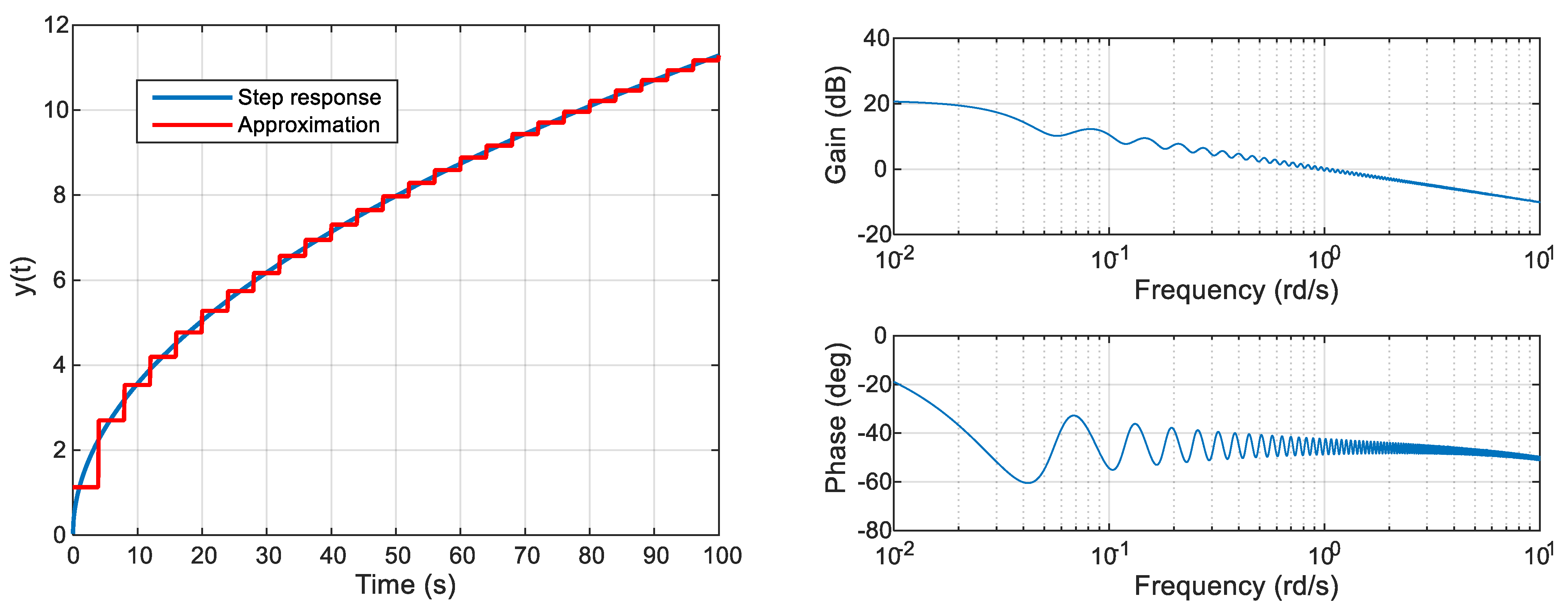
However, in the previous two approximations, the lag between two delays is not constant as in relation (17). To satisfy this constraint the following approximation can be used

$$s^{-\nu }\approx {\displaystyle \sum }_{k=1}^N{M}_k{e}^{-k{T}_{0}s}$$

(29)

with

$$M_k=\frac{y\left(\left(k+1\right)T_0\right)+y\left(k{T}_0\right)}{2}.$$

(30)

The accuracy of this approximation with a constant gap $T_0$ between two consecutive delays is represented by Figure 11 in the time domain (with $T_0=4 \mathrm{s}$, $\nu =0.5$) and in the frequency domain (with $T_0=0.02 \mathrm{s}$, $\nu =0.5$).

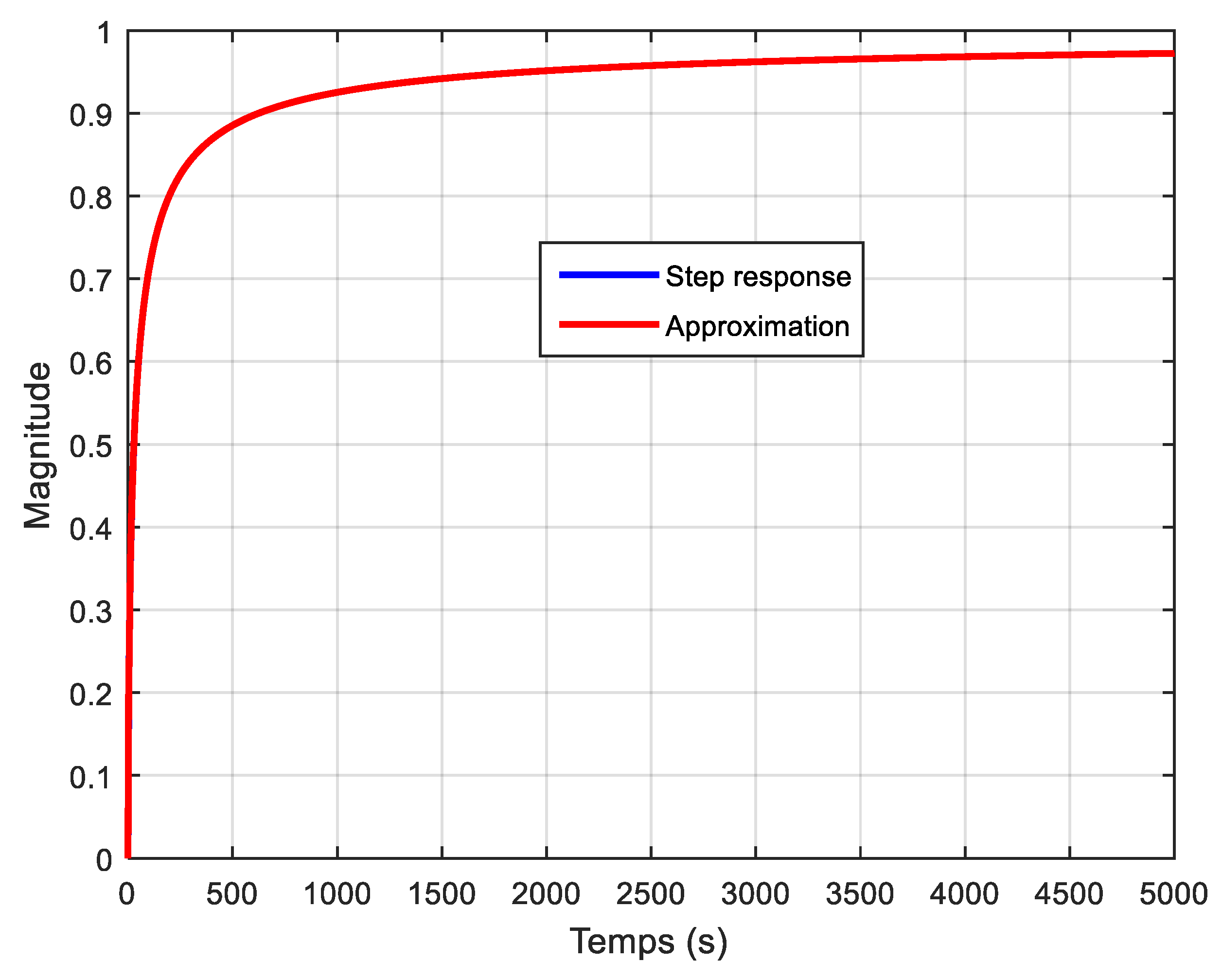
This approximation method and thus the associated probabilistic interpretation can be extended to numerous fractional transfer functions and behaviours. We have for instance

$$\frac{K_f}{1+\frac{s^{\nu }}{{\omega }_l}}\approx {{\displaystyle \sum }}_{k=1}^N{M}_k{e}^{-k{T}_{0}s}.$$

(31)

A comparison of the filter step response and its approximation is done in Figure 12 with $N=10000$, $T_0=0.5 \mathrm{s}$ $K_f=1$, ${\omega }_l=0.1$ rd/s and $\nu =0.6$. Note that the coefficients $M_k$ can be computed from the filter step response using relation (30) in which $y\left(t\right)$ denotes the filter step response. Thus, this approximation method can be applied directly to measures resulting from the step response of a real system exhibiting a fractional behaviour. It is interesting to see that this kind of approximation is close to the IIR filter-based approximations proposed in the literature for fractional transfer functions [36,37,38].

In relation (31), coefficients $M_k/K_f$ can be viewed as the probability to have a delay of duration $k{T}_0$ in the fractional behaviour studied as

$${{\displaystyle \sum }}_{k=0}^N\frac{M_k}{K_f}=1.$$

(32)

This probability distribution of $M_k/K_f$ as a function of $k$ ($k\in \left[1,100\right]$) for the transfer function of relation (31) is represented by Figure 13, again with $N=10,000$,$T_0=0.5 \mathrm{s}$, $K_f=1$, ${\omega }_l=0.1$ rd/s and $\nu =0.6$.

It must be noted that the idea of modeling fractional behaviors by means of a delay distribution was also used in another form in [39].

4.3. Adsorption Phenomena to Illustrate the Interest of this Probabilistic Delay Interpretation

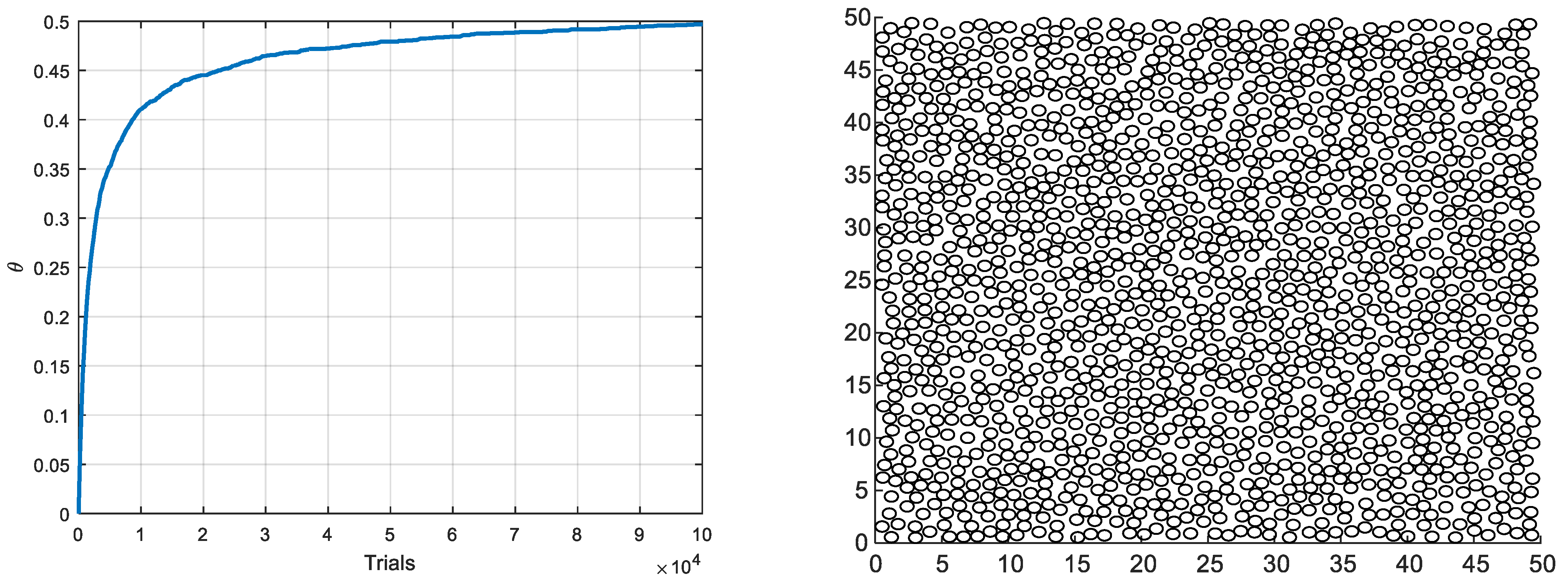
The adsorption phenomenon and the RSA process are again considered. The algorithm described in Section 4.1 for the RSA process is used to generate data with disk particles of radius $R=0.5$ that fall on a square with an edge length $L=50$. The response obtained in terms of surface coverage $\theta$ as a function of trials is shown by Figure 14, and will be denoted $\theta \left(t\right)$ in the sequel. This figure also shows the placement of the disks at the end of the process.

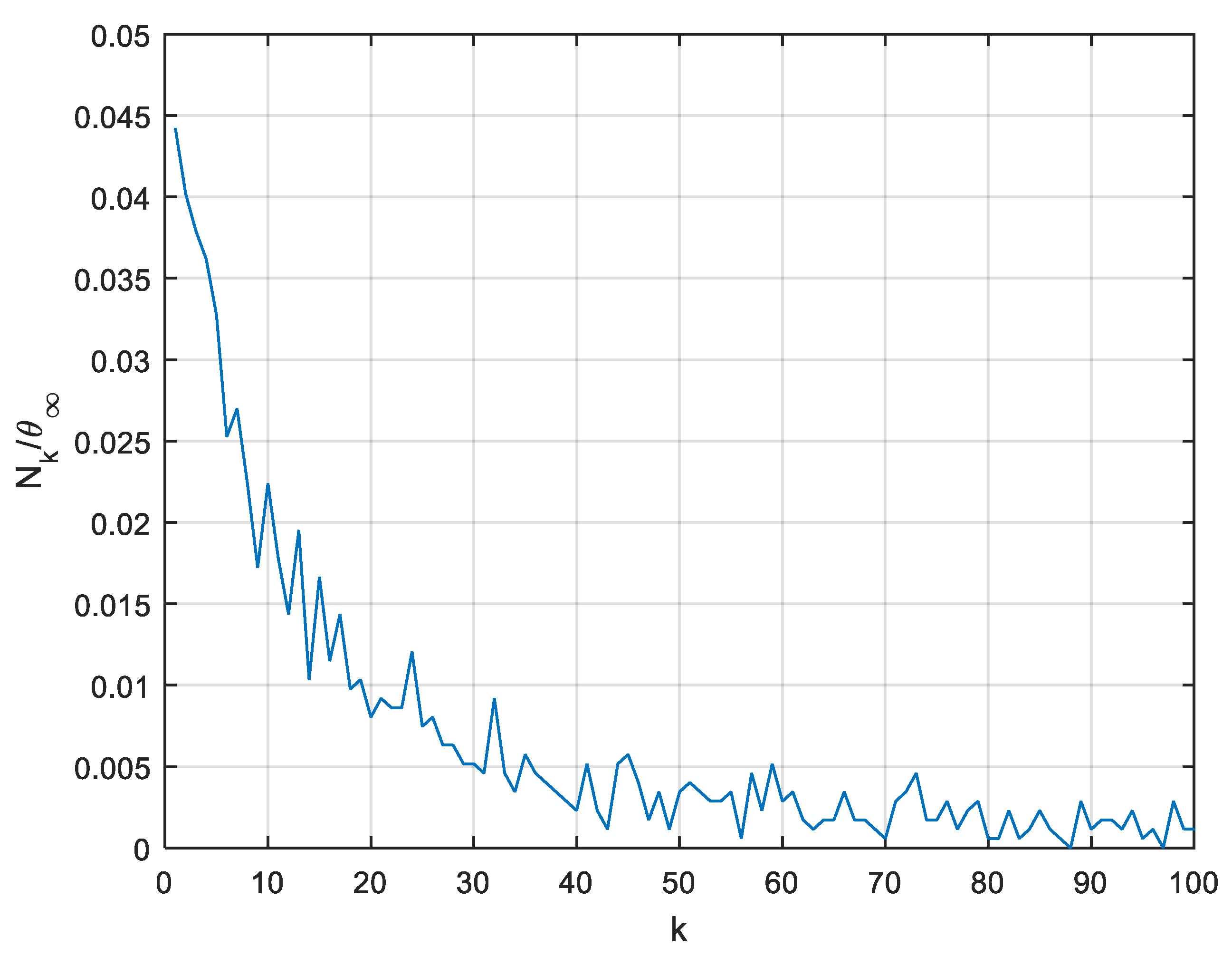
The response $\theta \left(t\right)$ can be approximated using a distribution of delay as in relation (31). The delay distribution is similar to the one presented by Figure 13. On the other hand, from the response $\theta \left(t\right)$, it is possible to compute the number of disks $N_k$ that find a place on the square in the time interval $\left[\left(k-1\right)T_0,k{T}_0\right[$. The numbers obtained are divided by ${\epsilon }_{\infty }$, the value of $\theta \left(t\right)$ when $t$ goes to infinity, which is close to 0.547 according to [31,32,33]. The resulting $N_k/{\epsilon }_{\infty }$ are then represented by Figure 15 as a function of k for $k\in \left[1,100\right]$.

One can note a very large similarity between Figure 13 and Figure 15, and thus between the values of $M_k/K_f$ and $N_k/{\epsilon }_{\infty }$. Consequently, the third probabilistic interpretation in terms of delay distribution leading to the expansion (31) has a physical meaning. The probability to find a time delay with duration $k{T}_0$ in the fractional behaviour produced by the RSA process is also the probability that $N_k/{\epsilon }_{\infty }$ disks find a place in the time interval $\left[\left(k-1\right)T_0,k{T}_0\right[$.

4.4. Another Example of Possible Physical Interpretation

The third statistical interpretation detailed in Section 4.2 which describes the probability that a delay is induced by a system that produces a given fractional behaviour may have other physical interpretations. This is the case for diffusion. It is well known that diffusion can be physically described through particle random walk [40]. It is also well known that diffusion produces fractional behaviours of order ½ or different from ½ in complex media such as fractal media [41]. But an interpretation based on delay distribution is also possible.

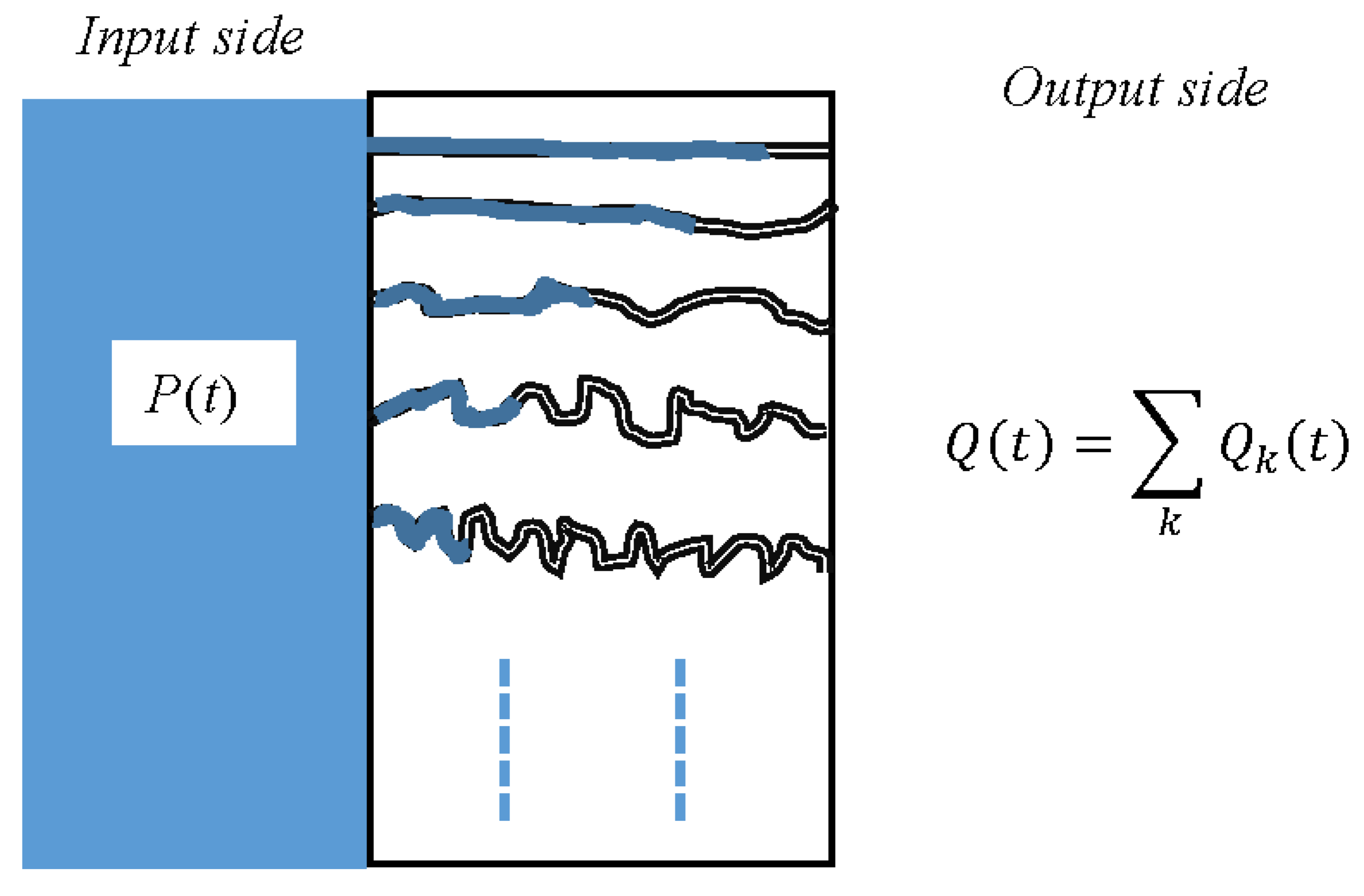
This interpretation is represented by Figure 16. The medium is assumed to be constituted of channels of various lengths. Before the water hits the medium, the channels are assumed to be empty of fluid. When the fluid pressure $P\left(t\right)$ appears at the input side, it creates a flow inside the channels such that the total flow at the output side denoted $Q\left(t\right)$ is the sum of the flow produced by each channel, denoted $Q_k\left(t\right)$:

$$Q\left(t\right)={{\displaystyle \sum }}_k{Q}_k\left(t\right).$$

(33)

The flow $Q_k\left(t\right)$ depends on the pressure $P\left(t\right)$ and on the inverse of the hydraulic resistance $R_k$ of each channel. Moreover, due to the difference in the channel length, each flow $Q_k\left(t\right)$ reaches the output side with a time delay $T_k$ depending on the channel length, thus leading for each $Q_k\left(t\right)$ to the relation:

$$Q_k\left(t\right)=\frac{1}{R_k}P\left(t-T_k\right)$$

(34)

and thus for the total flux:

$$Q\left(t\right)={{\displaystyle \sum }}_k\frac{1}{R_k}P\left(t-T_k\right).$$

(35)

If $Q_{\infty }$ denotes the steady state value of the flow $Q\left(t\right)$ when $P\left(t\right)$ is a unit step, then with such a modelling approach, it can be said that the coefficients $1/\left(Q_{\infty }{R}_k\right)$ can be viewed as the probability to have a delay of duration $T_k$ in the fractional behaviour produced by the diffusion phenomena. More physically, $1/\left(Q_{\infty }{R}_k\right)$ can be connected to a distribution of channel length and to the probability to find the corresponding channel in the studied system.

5. Conclusions

This paper proposes extensions of a probabilistic interpretation of fractional derivative operator that can be found in the literature [1]. The proposed interpretations are extensions because they concern other fractional operators and more generally fractional behaviours, and also by the nature of the random variables involved in these interpretations.

A first interpretation is derived from the impulse response of various fractional order transfer functions. These impulse responses are fitted with a distribution of time constants weighted by a function that can be interpreted as the probability to find these time constants in the system. However, this interpretation only gives a macroscopic view of what happens in a real system producing a fractional behaviour. Many systems that exhibit fractional behaviours are stochastic systems in that they are based on random and sequential kinetics of a multitude of agents in a constrained space. This is the case of adsorption or diffusion for instance.

A second interpretation is thus proposed. It is based on the approximation of a fractional behaviour using a distribution of time delays. The resulting probabilistic interpretation provides information on the probability of a given time delay to be present in a system. This interpretation is particularly interesting because it also allows a physical interpretation of the phenomena that take place in the system having a fractional behaviour. This is highlighted with the adsorption phenomenon that can be approximated by the RSA (Random Sequential Adsorption) process. RSA is a stochastic process in which particles sequentially incide a substrate at uniformly randomly chosen surface positions. A particle remains on the surface only if the target site is empty. As the substrate fills up, one has to wait longer and longer for a new disk to find its place. It is this notion of delay that is found in the second probabilistic interpretation proposed. This interpretation is also used to propose a physical interpretation of diffusion.

But this work is also a tribute to our colleague Professor Tenreiro Machado who was the first to propose in the literature a probabilistic interpretation of fractional derivative operator. Professor Tenreiro Machado, Dear José, we wish you were here, with us, to discuss again these probabilistic interpretations.