
Fisher-like Metrics Associated with ϕ-Deformed (Naudts) Entropies
by
 , , and
Cristina-Liliana Pripoae
1 ,
,
Iulia-Elena Hirica
2,
Gabriel-Teodor Pripoae
2,* and
Vasile Preda
2,3,4 1
Department of Applied Mathematics, The Bucharest University of Economic Studies, Piata Romana 6, RO-010374 Bucharest, Romania
2
Faculty of Mathematics and Computer Science, University of Bucharest, Academiei 14, RO-010014 Bucharest, Romania
3
“Gheorghe Mihoc-Caius Iacob” Institute of Mathematical Statistics and Applied Mathematics of Romanian Academy, 2. Calea 13 Septembrie, nr.13, Sect. 5, RO-050711 Bucharest, Romania
4
“Costin C. Kiritescu” National Institute of Economic Research of Romanian Academy, 3. Calea 13 Septembrie, nr.13, Sect. 5, RO-050711 Bucharest, Romania
*
Author to whom correspondence should be addressed.
Mathematics 2022, 10(22), 4311; https://0-doi-org.brum.beds.ac.uk/10.3390/math10224311
Submission received: 12 October 2022
/
Revised: 5 November 2022
/
Accepted: 15 November 2022
/
Published: 17 November 2022
(This article belongs to the Special Issue Probability, Stochastic Processes and Optimization)
Abstract
:The paper defines and studies new semi-Riemannian generalized Fisher metrics and Fisher-like metrics, associated with entropies and divergences. Examples of seven such families are provided, based on exponential PDFs. The particular case when the basic entropy is a -deformed one, in the sense of Naudts, is investigated in detail, with emphasis on the variation of the emergent scalar curvatures. Moreover, the paper highlights the impact on these geometries determined by the addition of some group logarithms.
Keywords:
ϕ-deformed (Naudts) entropy; divergence; relative group entropy; generalized Fisher metric; Fisher-like metric; MaxEnt problemMSC:
53B12; 22E70; 94A17; 53B201. Introduction
1.1. History
Entropy is a a very versatile measure of order (or of chaos). In the last few several decades, the growing needs of modeling for stochastic phenomena contributed to the apparition of many new different families of entropy functionals, with increasing levels of generality, reliability and applicability [1,2,3,4,5,6,7,8,9,10,11,12,13,14,15,16,17,18,19]. One of the recent interesting new directions of study uses the relative group entropies, based on group logarithms (see [20,21] and references therein).
The geometrization method, a powerful tool in modelization, was applied in the investigation of some statistical relevant parameters sets, beginning with the work of the pioneers: Fisher, Rao, Efron and Amari [12,22,23]. This bridge allows the use of the differential geometric machinery to understand the local and the global behavior of statistical objects.
In particular, the Fisher (semi-Riemannian) metrics correspond to the Fisher Information matrices. Their invariants, especially those tensor fields expressing different kinds of curvature properties, are used in the parameters estimation theory as control tools. For example, the scalar curvature function measures the average statistical uncertainty of a density matrix [12,20,24].
Consider a statistical model, governed by a given entropy, and two or more fixed parameterized probability density functions (PDFs) within it. Various divergences (“distance-like functionals”) can be defined in this framework, able to detect how these PDFs relate to each other. A kind of infinitesimal variation of such divergences, w.r.t. the parameters, may provide interpretations for some Fisher-like metrics. Several types of divergences are used, including the Kullback–Leibler and the Bregman ones. For recent viewpoints upon divergences, see [14,25,26].
In 2002, Naudts introduced ([27]) the “-deformed entropy”, via a positive strictly increasing function , which plays the role of a “generalized logarithm”. (We shall call it “-deformed (Naudts) entropy” and not simply “-deformed entropy”, in order to avoid confusion and to distinguish it from other “deformed” entropies, all originating—sooner or later—from the Boltzman–Gibbs–Shannon (BGS) germ). This new entropy extends (with some technical precautions) the Tsallis and the Kaniadakis entropies, among other ones. Using it, new Fisher metrics were defined [27,28,29], ranging from simple ones to some more “baroque” constructions. Their applicability covers a wide area, from Physics (the starting point) to Information geometry [29,30,31,32].
Using a -deformed (Naudts) exponential family of PDFs, Matsuzoe et al. [33] investigated the geometry of statistical manifolds derived from a sequence of escort expectations.
Korbel et al. [30] studied properties of the Fisher metrics associated with the -deformed (Naudts) entropies, in the case of exponential-type PDFs. Particular choices of the function provided examples based on -entropies. Dealing with the MaxEnt problem, they use the Fisher information of the -deformed (Naudts) exponential entropies, in order to reveal a duality between the cases with linear constraints and those based on escort constraints.
Inspired by these previous works, we believe that a systematic study of semi-Riemannian metrics, canonically associated with the -deformed (Naudts) entropy, is necessary and might provide useful statistical tools in the future. Our paper suggests a method of research, which combines the beaten path with some new speculative ideas.
1.2. The Content of the Paper
In Section 2, we recall (in a creative manner) the notations and fix the conventions concerning (the different variants of) entropy and divergence; we closely follow [34]. We make some comments about the place of the Naudts’ -deformed entropy in the “Universe” of generalized entropies. We recall here some other examples of remarkable entropies (Tsallis, Kaniadakis, Sharma–Taneja–Mittal). Our main new idea is the distinction we made between the “quotient” divergence and the “difference” divergence, in the context of generalized logarithms; in the particular case of the Neperian logarithm, these two notions coincide, but in other cases (such that of the -deformed (Naudts) entropy) they are distinct.
In Section 3, we fix the needed notions concerning the generalized Fisher-like metrics associated with the entropies and to the relative (group) entropies, following (especially) [20]. Following the previous distinction we made in Section 2, between the two kinds of divergences, we introduce two generalized Fisher-like metrics (GFM1 and GFM2), which coincide in the classical setting with the Fisher metric. Three other Fisher-like metrics are defined, in a formal way, as auxiliary (but eventually useful) by-products of the former ones.
In Section 4, we determine the semi-Riemannian geometries of the generalized Fisher-like metrics, associated with group relative entropies based on -deformed (Naudts) entropies and divergences. Their coefficients are expressed in terms of both PDFs and of the -deformed logarithm and may depend on a group logarithm too.
In the next section, we give seven families of examples of such metrics, for the case when the involved PDFs are exponential. The scalar curvatures functions are computed, and their variation is studied.
In Section 6, we define and solve the MaxEnt problem based on the -deformed (Naudts) entropy, for univariate PDFs, and we generalize some thermodynamic relations.
1.3. Conventions
Implicitly, the integrals are supposed to be correctly defined and to commute with their derivatives. “Differentiable” means “smooth”, even if, sometimes, a weaker assumption would be enough. When a symmetric matrix is called “a (semi-Riemannian) metric”, we assume, implicitly that it is non-degenerate; the positive definiteness is not assumed, in general, unless otherwise stated.
2. Entropies and Divergences—A Breviary
We consider a real valued random variable x on a domain . We denote by a fixed probability density function (PDF); then, and . We fix a real valued differentiable function , as a “controlling tool”. In this setting, the generalized (normalized) entropy is
We shall use a similar notation for other entropy-like functionals too. In the literature, the avatars of the “generalized logarithm” are subject to additional restrictions, imposed through applications inspired axioms.
Let a smooth function and an additional fixed PDF. We define
We suppose that and if and only if . The number is called the (generalized) divergence between and and measures to what extent influences . Sometimes, additional properties of the divergence function are added, axiomatically.
Example 1.
(i) In the particular case when , from Formula (1), we obtain the Boltzmann–Gibbs–Shannon (BGS) entropy.
(ii) Consider a fixed parameter . The Tsallis q-logarithm
provides a Tsallis entropy. Usually, for , we use the notation . When , the BGS entropy is recovered.
(iii) Let us fix . The Kaniadakis k-logarithm
defines a Kaniadakis entropy (named also k-deformed entropy). Usually, is denoted . When , we recover again the BGS entropy.
(iv) Fix two real parameters k and r. The Sharma–Taneja–Mittal -logarithm
provides a Sharma–Taneja–Mittal (STM) entropy (also named -deformed entropy). Instead of , we shall denote . The Kaniadakis k- logarithm and the Tsallis q-logarithm are recovered as particular cases, for and for , respectively. When , we recover the BGS entropy. Sometimes, additional restrictions are imposed on the domain of the parameters, required by convergence conditions imposed on some integrals (see [38,39,40] for details).
(v) ([27]) Let a positive, differentiable, strictly-increasing function. (Sometimes, in the literature, “non-decreasing” is required, instead of the “strictly-increasing” condition). Define the ϕ-deformed (Naudts) logarithm
The function defines the ϕ-deformed (Naudts) entropy. The previous formula may also be read “backwards”:
Moreover, given an arbitrary “generalized logarithm” φ as in (1), Formula (6) always provides a differentiable function ϕ; if it is positive and strictly-increasing, we expressed φ like a ϕ-deformed (Naudts) logarithm. Sometimes, this procedure works for some restrictions of the involved parameters only. For example, the preceding four entropies are recovered as particular cases of ϕ-deformed (Naudts) entropies, as follows: BGS for ; Tsallis for with the restrictions and ; Kaniadakis with the additional restriction
for ; STM for
with the additional restriction
for . These additional restrictions are imposed in order ϕ to be strictly-increasing.
(vi) Let be a formal group logarithm, which is a differentiable real valued function with some special algebraic properties, inspired from the formal series linking Lie groups to Lie algebras. More precisely,
where and . Its inverse is
where , , , and so on. (We refer to [20,21,41] for details about these functions). The simplest example is .
We define the generalized group entropy functional (GGEF) associated with (1) by
In particular, for , we recover the well-known group entropy functional ([20,41]) associated with (1)
Similar GGEFs can be provided by replacing the Neperian logarithm by other “generalized” logarithms (e.g., Tsallis, Kaniadakis, STM, etc). In Section 3, we shall introduce the geometries associated with the GGEF, based on ϕ-deformed (Naudts) entropies. Accordingly, we shall use the generalized logarithm from (5).
Example 2.
With the previous notations, we recall some well-known examples of divergences.
(i) An important particular case is the generalized (quotient) relative entropy (a.k.a. generalized divergence) between ρ and σ (see [34,42])
The function . We accept (formally) that , and . In particular, when , we recover the Kullback–Leibler divergence ([20]).
Another particular case considers to be a convex function, with and . For , we recover the f-divergence ([43] and references therein). The slightly more general notion of -divergence (see [44]) may be recovered in a similar way.
(ii) In a similar way, we define the generalized (difference) relative entropy between ρ and σ, as
The function . In particular, when , coincides with D and we recover the Kullback–Leibler divergence, as in (i). When , the divergence D was considered in [27]; we mention that, in this case, does not coincide with D.
In general, a necessary and sufficient condition on φ, ρ and σ, in order that , is the vanishing of the mean function . A sufficient (but quite strong) condition is provided by the functional equation .
(iii) In the hypothesis of Example 1 (vi), we can define generalized divergences as relative group entropies, which combine the formal group logarithm G, the φ-likelihood function and the previous quotient or difference operation upon two PDFs. For example, the analogue of (10) is
(iv) Consider two fixed PDFs and . Denote as a fixed convex differentiable function. In this setting, the Bregman divergence is
We mention that the function is convex too.
Let be a time-dependent PDF, where . Then, the entropy in (1) will also depend on the parameter t, so . We consider a potential energy function and its associated energy average function
(If needed, restriction of these functions to open subsets is possible). This particular framework will be used in Section 6 only.
3. Fisher-like Metrics Associated with Generalized Entropies and Generalized Divergences
In this section, we recall the notion of Fisher metric associated with a family of (generalized) entropies or divergences, defined on the space of parameters of an arbitrary PDF, using mainly [20,34]. For a more general setting, see [34].
Consider the case when the PDF in Section 2 depends, moreover, on n real parameters , with , where is an open set of . Thus, , . Let be a differentiable controlling function, . The dependence on leads to a generalized entropy function , canonically derived from Formula (1):
In a similar natural way, we can define generalized divergence functions, by -parameterizing (2) and its avatars.
Define
and
We suppose that the matrices and are non-degenerated, and g has constant index on . We call g and generalized Fisher metrics of type 1 and type 2, respectively, and denote GFM1 and GFM2. Both metrics are “means”, w.r.t. , of some -mediated “information matrices”: the Hessian of and the matrix of the gradient of with its transpose, respectively. The diagonal coefficients , , generalize the Fisher Information Numbers from [45], which can be recovered when is the Tsallis logarithm.
In general, the semi-Riemannian metric g and the Riemannian metric differ from each other and differ from the Hessian (semi-Riemannian metric if non-degenerated)
We define, in a formal way, two auxiliary symmetric tensors of (0,2)-type and , given by
and
We remark that, if non-degenerated, and provide semi-Riemannian metrics. In this case, these metrics are also of Fisher type, as they express “means” w.r.t. the PDF of two “derived information matrices”, of coefficients and , respectively.
Example 3.
Consider the particular case of the BGS-entropy, with .
(i) In this case, both previous GFM1 and GFM2 coincide with the classical (Riemannian) Fisher metric associated with H (or φ) [20].
In the general case, it would be interesting to find all the controlling functions φ, for which g coincides with . Does this property necessarily imply that φ is proportional with , modulo a non-null constant? A further step would be to look for appropriate functions φ, in order that g and : be homothetic or conformal; have the same geodesics; have the same curvature, etc. To this differential geometric viewpoint, a statistical counterpart may eventually correspond.
(ii) Let be an open set and let , , …, , be smooth functions on X. Consider the PDF of exponential type, given by
The associated Fischer metric is , which is a Hessian metric.
(iii) For this choice of the function φ, we obtain and , for . The “perturbed” Hessian matrix associated with α is similar to the one studied in some recent statistical applications (see, for example, [46]).
Remark 1.
(i) We give an interpretation and a motivation for the definition of the GFM1, in a slightly more general case than [20]. Consider φ a fixed controlling function. Let and be two families of parameterized PDFs over , with , and let
be the generalized (difference) relative entropy between them, as in (10). Denote and suppose its norm to be infinitesimally small. We know that has a unique minimum for , i.e., for . The Taylor decomposition around gives
The second order approximation of this expression is precisely half of the GFM1 g, calculated in .
When , we recover the interpretation given in [20].
(ii) We do not know a similar interpretation for the GFM2 .
(iii) The generalized group relative divergences from Example 2 (iii) provide analogous formulas. We shall study them in the next section, in the particular case of the ϕ-deformed (Naudts) entropy.
(iv) The definition of Fisher metrics described previously is closely related to the need for understanding a variation of a PDF w.r.t. another (reference) one; the output of this “variational calculus factory” are functions. We signal here the forthcoming book [47], containing new revolutionary ideas in Variational calculus, including invariants of tensorial type, motivated by differential geometric problems; this source provides new insights for the definition and the study of divergence-like tensor fields, as a path toward a new bundle spaces approach in Statistics.
(v) All the previous tensor fields g, , h, α, and β have constant index, one each connected component of their definition domains.
An open problem is to find the more general hypothesis such that these tensor fields be non-degenerated (in order to define semi-Riemannian metrics). Locally, the answer is simple: let be a point in the parameters space, such that the determinant of the corresponding matrix, calculated in , is not null. Then, the tensor field is non-degenerated in an open neighborhood of . For many families of examples (and in Section 5 we add several more ones), this property holds true. A common practice in the literature is to stop here, without investigating global conditions which are fulfilled in general cases. To our knowledge, global existence results for Fisher metrics, in the general setting, are not proven yet. Moreover, the eventual singular points have an interest in their own, as they may signal—in a suitable statistical model—a phase transition ([48]).
We consider it useful to point out here the paper [49], where a different but correlated problem is studied: namely, to what extent the Fisher metric is (globally) unique, modulo the action of a diffeomorphism group.
4. The Fisher Geometries Associated with GGEFs Based on -Deformed (Naudts) Entropies and Divergences
We particularize now the results from Section 3, for the case of the Naudts entropies. Let us fix the context more precisely.
Consider a positive, differentiable and strictly-increasing function as in Example 1 (v) and the -deformed (Naudts) logarithm defined in Formula (5). Let , be a family of parameterized PDFs, as in Section 3. The associated GFM1 g and the GFM2 are obtained as particular cases from (14) and (15):
and
We suppose, as usual, that g and are non-degenerated and that has a constant index on X.
We also consider, via (16), the associated Hessian metric
Proposition 1.
With the previous notations, for every , we have
and
In this case, and are given by
and
Corollary 1.
In a condensed form, we have the following relation
We consider now, in addition, a fixed formal group logarithm G, as in Example 1 (vi). Let be the associated parameterized PDFs and be the generalized (difference) group relative entropy (a.k.a. the generalized (difference) group divergence), as particularization from (10) and Remark 1 (i), (iii), written as
Denote the generalized group Fisher metric associated with by
This Hessian-type metric will be calculated in the next result.
Proposition 2.
With the previous notations, we have the relation
which may be re-written as depending only on ϕ and ρ, in
Proof.
Suppose, for the moment, that is constant. Denote
Suppose, moreover, that . Then, we have
We re-write this formula in a condensed form, and we obtain the following result, which completes Corollary 1.
Corollary 2.
With the previous notations, for , we obtain
By analogy, starting with a generalized (quotient) group relative entropy (a.k.a. the generalized (quotient) group divergence) , as particularization from (9), we shall obtain, in the sequel, other Fisher-like metrics, similar to the ones in Proposition 2 and Corollary 2.
Denote the generalized group Fisher metric associated with by
Proposition 3.
With the previous notations, we have the relation
where denotes the classical Fisher metric.
Proof.
We adapt the proof of Proposition 2, from the divergence to the divergence . Suppose that is constant. Denote
It follows that
and
We assign , and we use the property . We obtain
The first integral equals . The second integral is null because . We obtained Formula (30). □
Remark 2.
(i) In Proposition 1, we establish the basic formulas for the future development of associated Riemannian geometries determined by g, , h, α, β, in terms of the function ϕ-deformed (Naudts) entropy (curvature, geodesics, Riemannian distance in the positive definite case). Examples of scalar curvature functions derived from these formulas will be shown in the next section. The coefficients of GFM1 g extend known ones from [29], derived for PDFs of exponential type and for particular functions ϕ. The other Fisher metrics are new.
An interesting consequence of Proposition 1 is the fact that g and do not coincide, as in the case of the Neperian logarithm. This can be seen directly, by comparing their ϕ-dependent coefficients.
(ii) In Proposition 2, we derive the Fisher-like metric associated with the divergence , as a generalization of a construction in [30] for the case of a Kullback–Leibler divergence, of a trivial group logarithm and for PDFs of exponential type.
(iii) In Proposition 3, the Fisher-like metric associated with the divergence is—to our knowledge—completely new.
The metrics in Formula (30) are homothetic, via a constant supposed—implicitly—to be not null. It is interesting that depends only on the behavior of the deformation function ϕ, for or around 1 and on G, around 0. Its independence on the PDFs gives an “universality” feature, which corresponds—probably—to some special uncovered property of the statistical model.
Suppose, moreover, that . We replace in (30) the values and , and we obtain
5. Examples
We particularize now the results from Section 4, for the case when is an exponential PDF and , . The deforming function will be chosen conveniently, in order to be able to compute the integrals.
Let and be the exponential (normal) PDF given by
We denote the partial derivatives of , with respect to the variables and , by , , , , . A short calculation ([34]) leads to the formulas
For future calculations, we shall use the following simple result.
Lemma 1.
Let c, , be fixed real constants, with , . Then, the semi-Riemannian metric
on the set in has the scalar curvature
In the sequel, we give examples of the semi-Riemannian metrics from Propositions 1–3, under various particular assumptions.
I—The case of g. Suppose , with an arbitrary fixed parameter. From Formula (22), we calculate the coefficients
where
There exists a unique such that . For this value, g is degenerated. The metric g is Lorentzian, when and is Riemannian, when .
The scalar curvature of g is
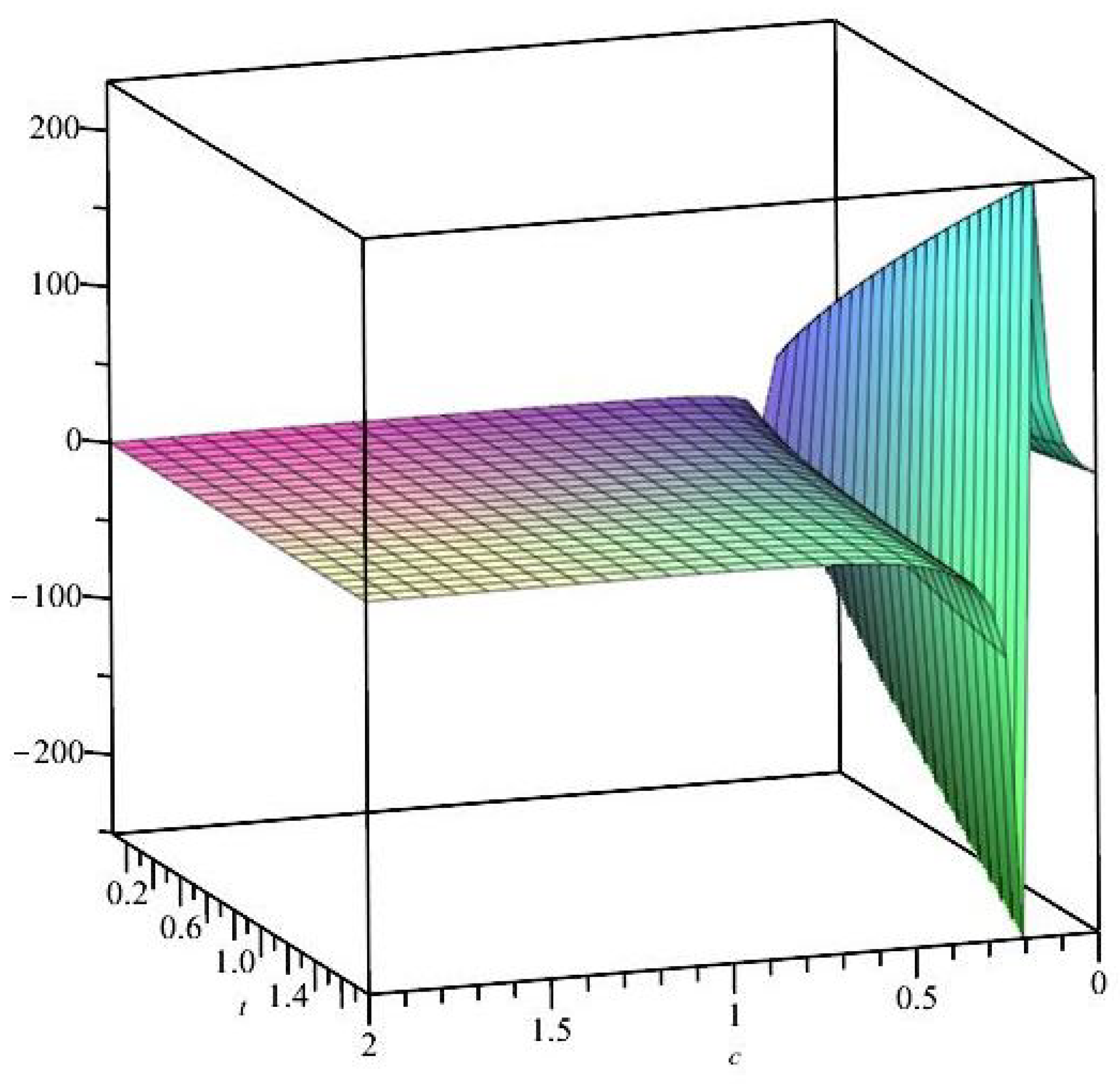
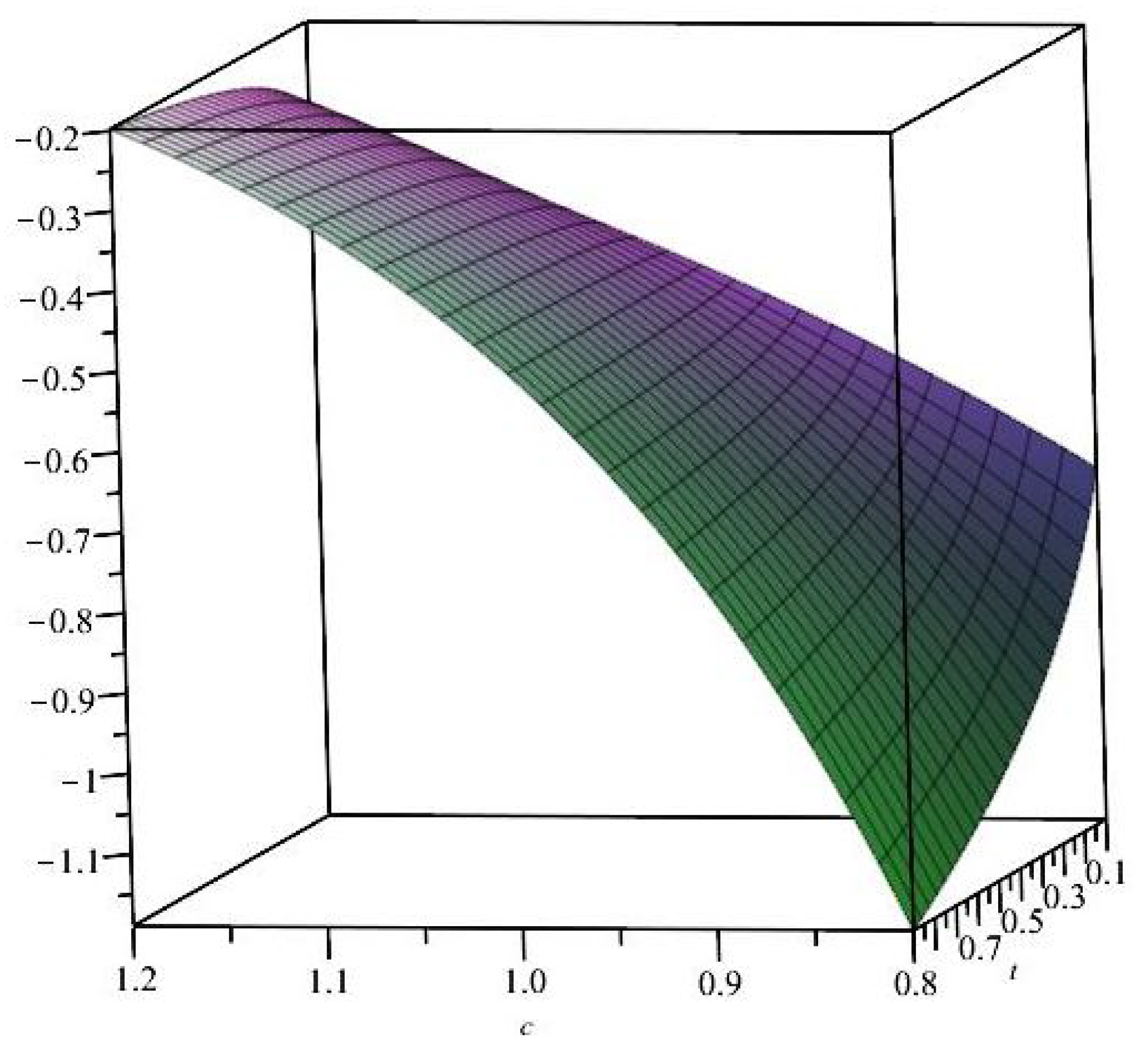
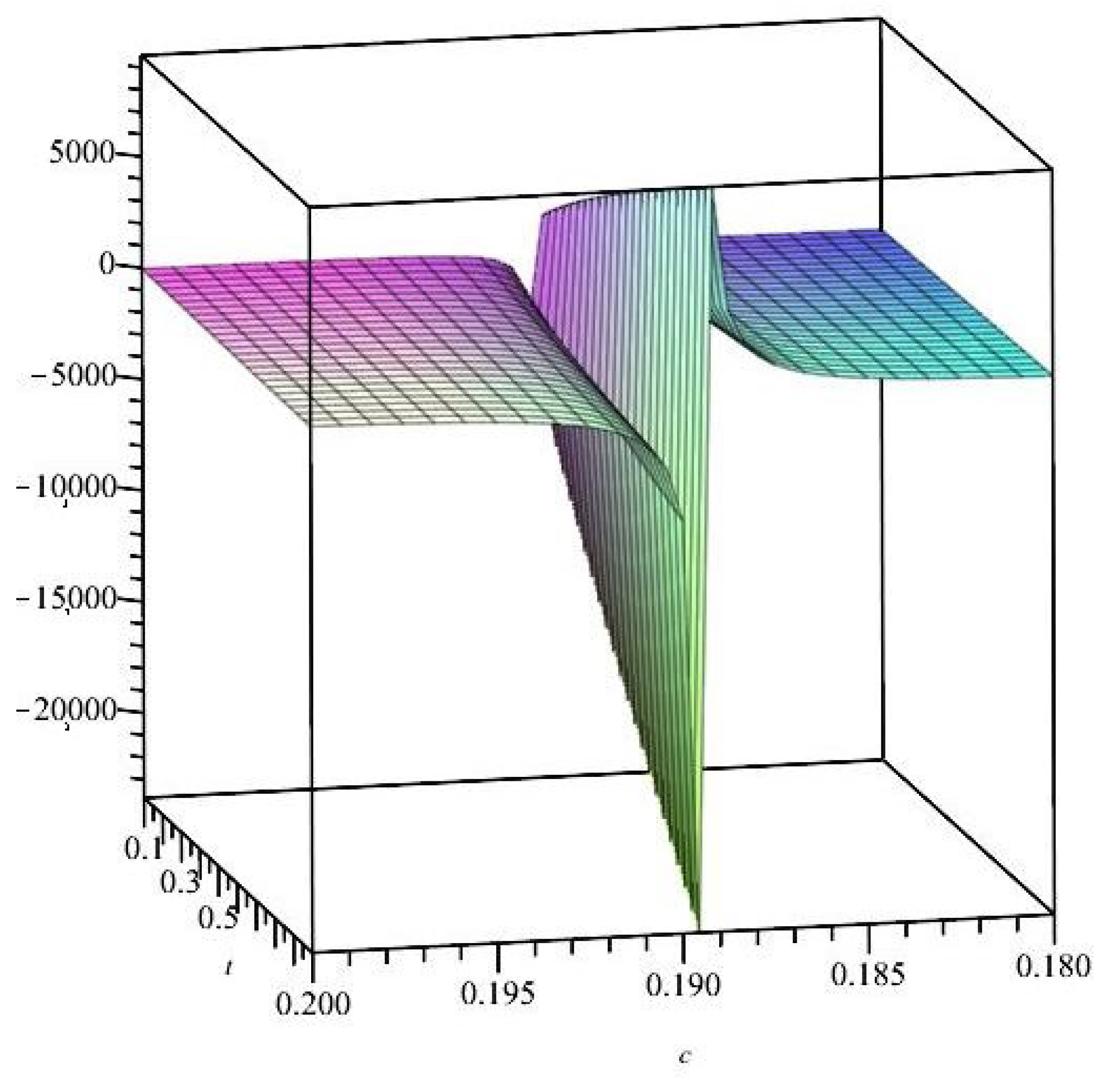
The scalar curvature does not vanish anywhere, and its sign is the opposite sign of . Moreover, is constant if and only if , i.e., only in the case when g is the classical Fisher metric . If we decide to use the scalar curvature as a control, this may lead to a quick criterion to distinguish the BGS entropy case from the -deformed (Naudts) entropy case. (The statistical interpretation of the scalar curvature of the Fisher metrics may be found in [20]).
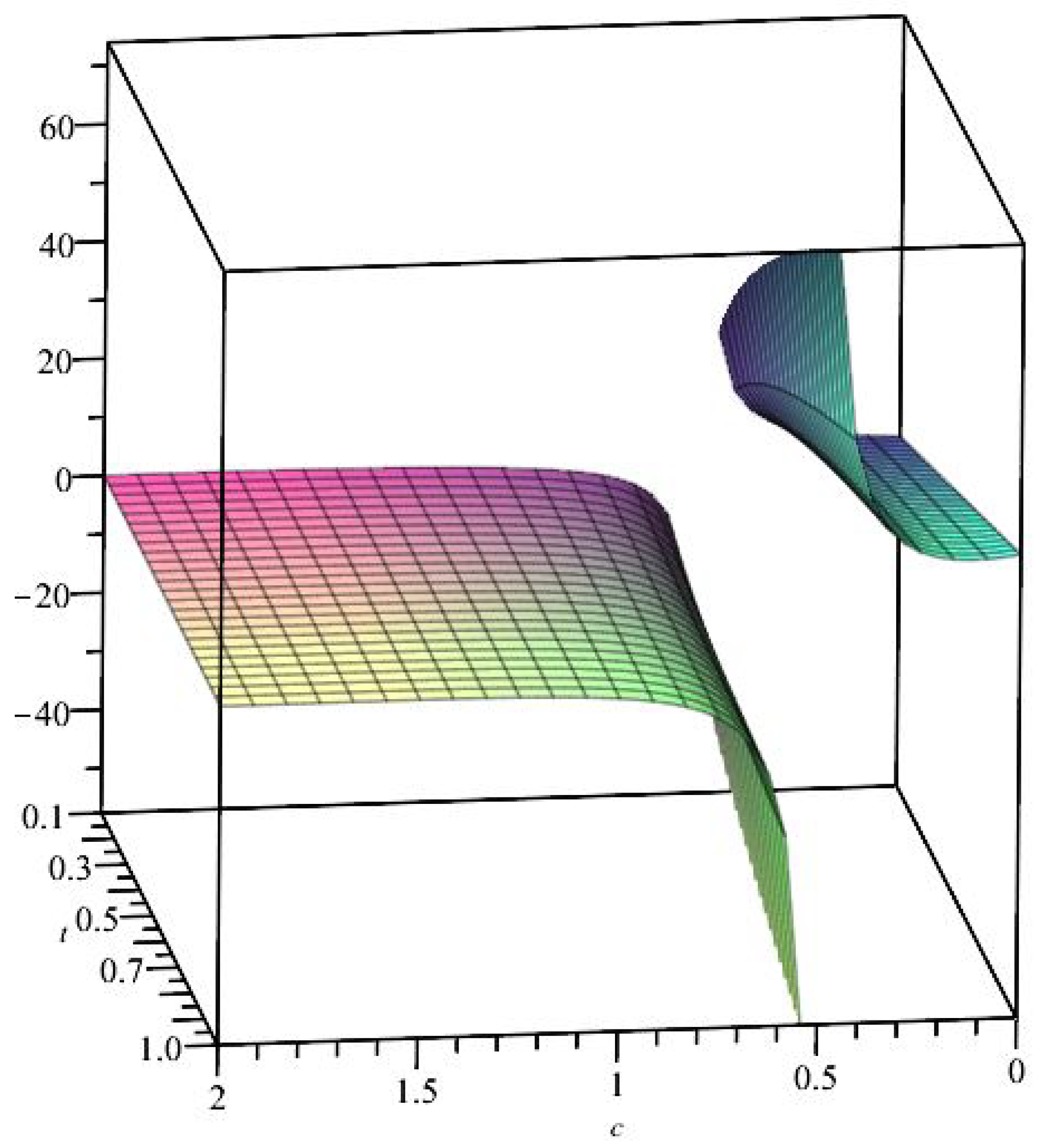
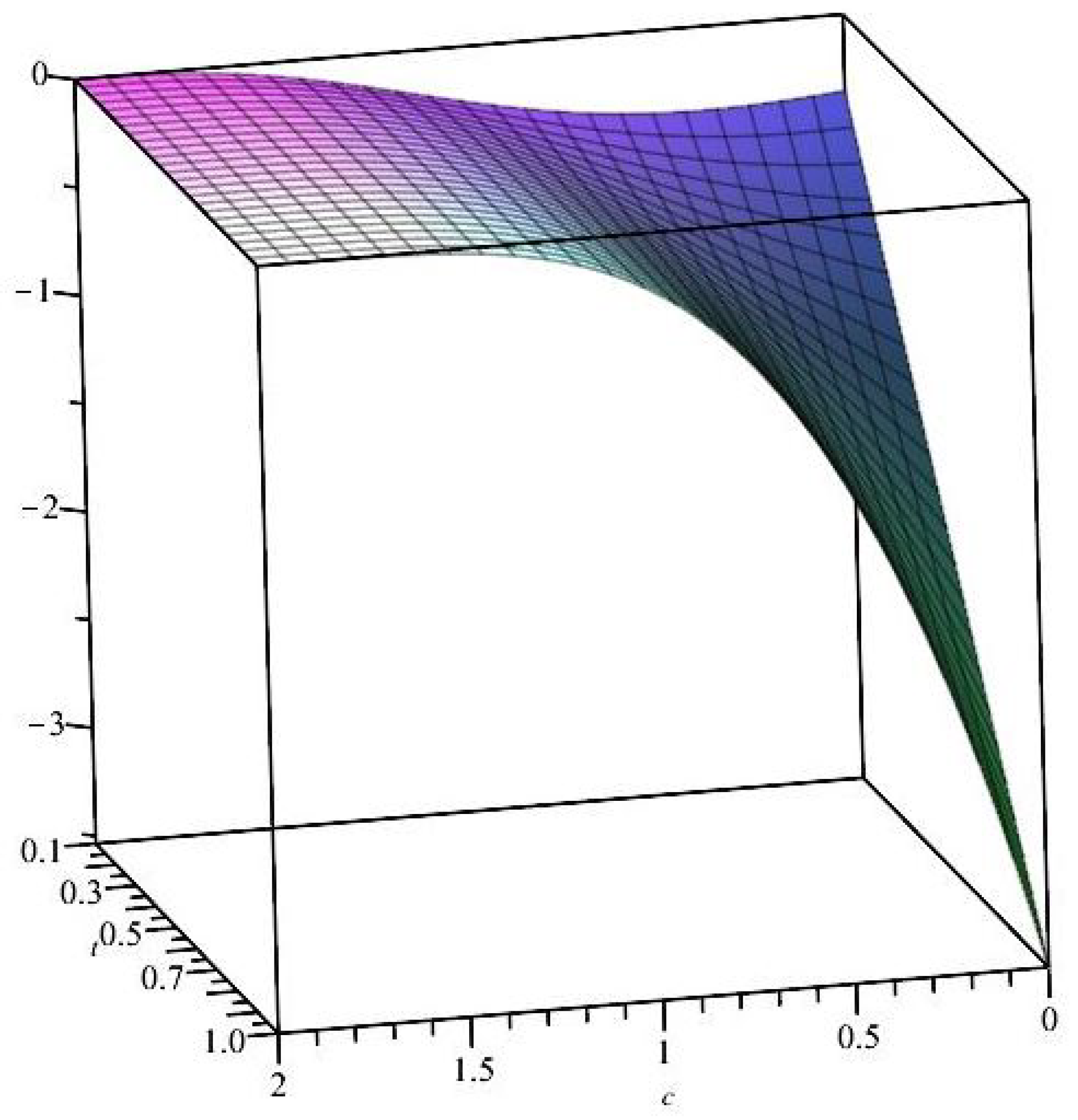
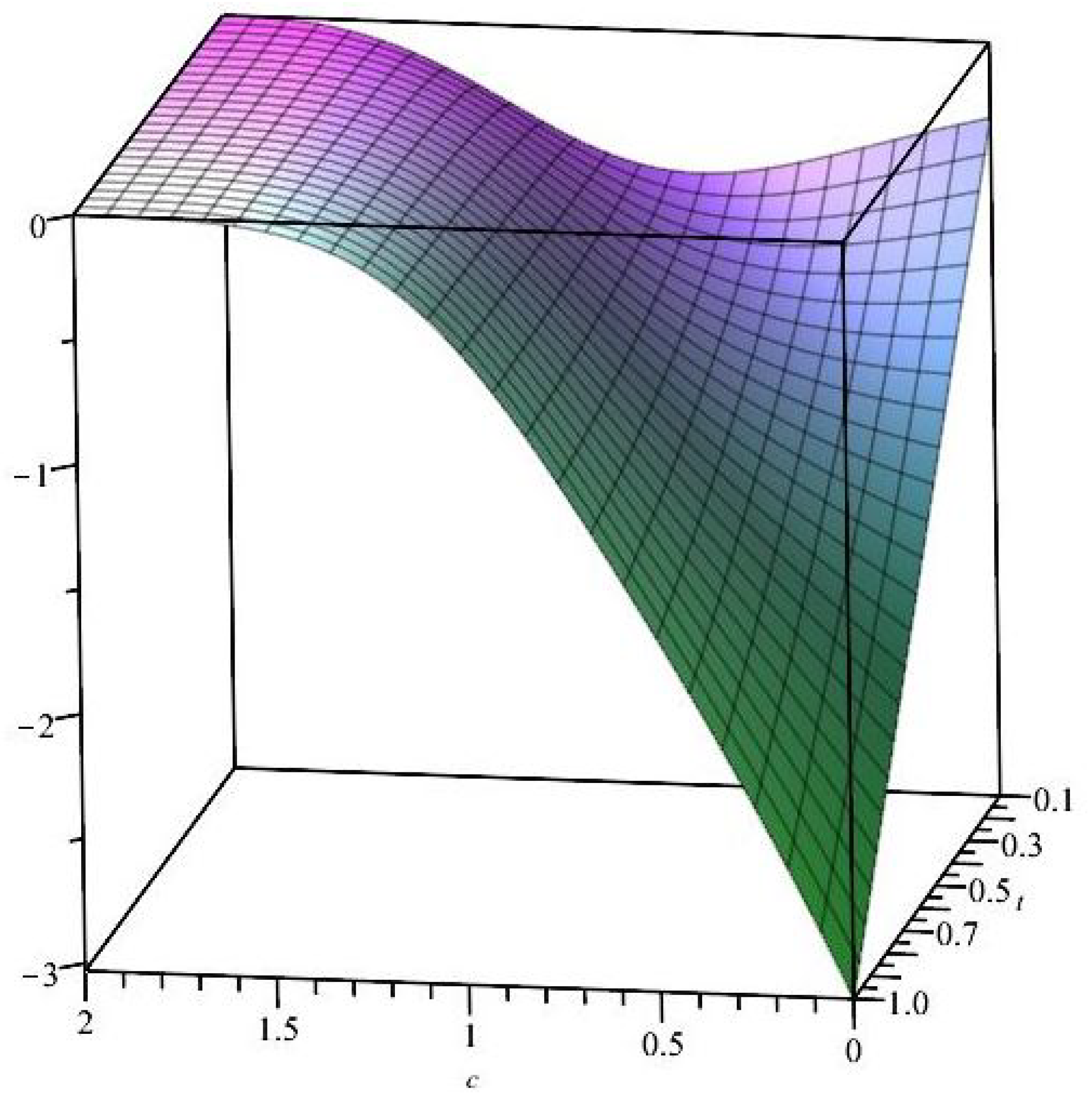
We depicted in Figure 1 (and magnified in Figure 2 around and in Figure 3 around ) how varies w.r.t. c and (denoted t).
II—The case of . Suppose , with an arbitrary fixed parameter. From Formula (23), we calculate the coefficients
where
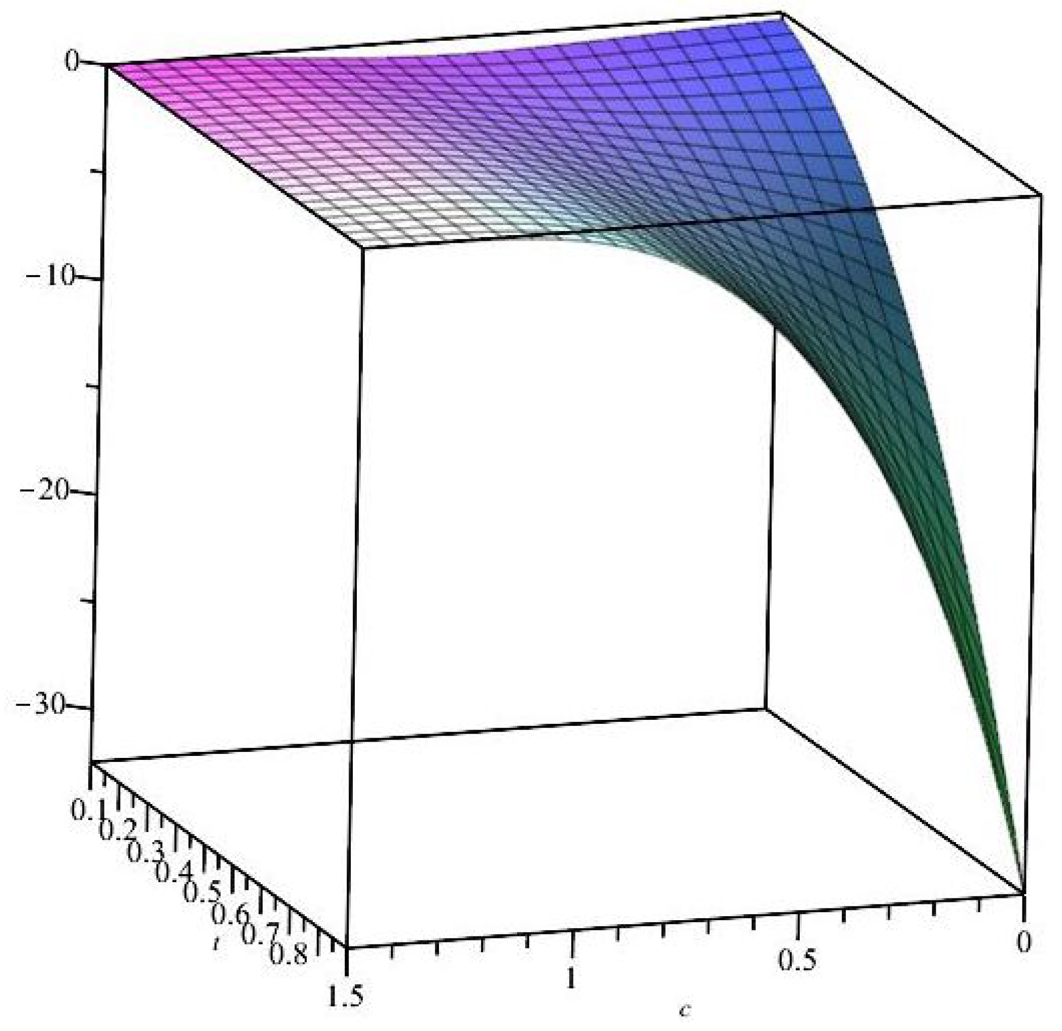
The scalar curvature of the Riemannian metric is
We mention that: the scalar curvature is negative; it decreases indefinitely as the variable grows and the parameter c goes to 0; it tends to 0 as c goes to . We depicted in Figure 4 how varies w.r.t. c and (denoted t).
III—The case of h. Suppose , with an arbitrary fixed parameter. From Formula (24), we calculate the coefficients
where
As the (0,2)-type tensor field h is degenerated, it does not define a semi-Riemannian metric. In this case, there is no scalar curvature to compute.
IV—The case of . Suppose , with an arbitrary fixed parameter. From Formula (17) or from Proposition 1, we calculate the coefficients
where
The (0,2)-type tensor field is degenerated for . If , then is a Lorentzian metric. If , then is a Riemannian metric.
The scalar curvature of is
and has the sign of . We depicted in Figure 5 how varies w.r.t. c and (denoted t).
V—The case of . Suppose , with an arbitrary fixed parameter. From Formula (18) or from Proposition 1, we calculate the coefficients
where
The scalar curvature of is
and takes negative values. We depicted in Figure 6 how varies w.r.t. c and (denoted t).
VI—The case of . Suppose , with an arbitrary fixed parameter. From Formula (27), we calculate the coefficients
where
We suppose that the group logarithm G is chosen such that be non-degenerated. The scalar curvature of is calculated using MAPLE:
Interestingly, the scalar curvature is a rational function of and .
We particularize now the setting for the BGS group logarithm and replace and in the previous formulas. Then,
where
In this particular case, the scalar curvature of the Riemannian metric has the form:
(The same formula may be recovered, directly, by using Lemma 1.) We mention that takes negative values, for every . In Figure 7, we depicted how this particular varies w.r.t. c and (denoted t).
For the moment, we suppose that G and are suitable chosen, such that . It follows that is a Riemannian metric. As the scalar curvature of is a negative constant , we deduce the scalar curvature of is a negative constant w.r.t. too. In what follows, we study the variance of in two particular cases.
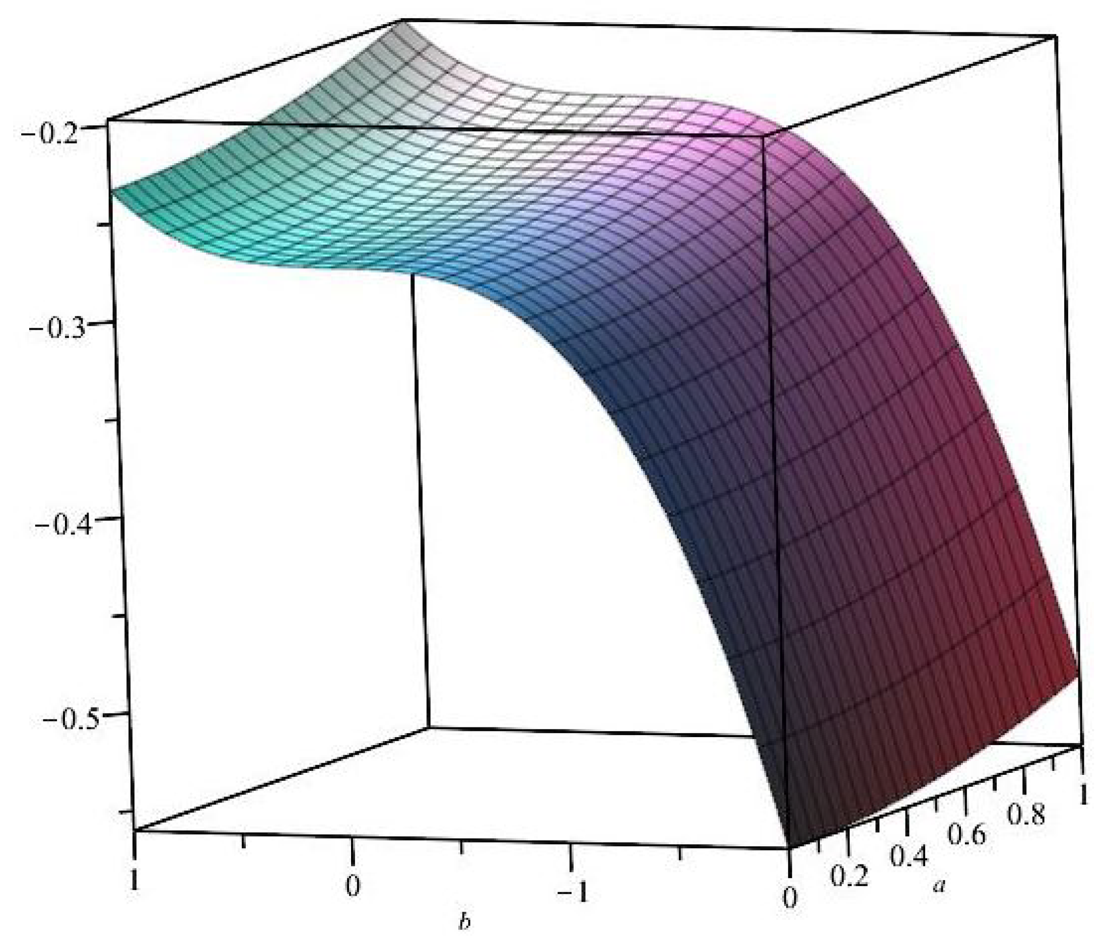
. Let be the BGS grup logarithm function and consider , where the real parameters a and b satisfy . Denote the respective metrics by and their scalar curvatures by . Then,
The family of Fisher-like Riemannian metrics may be considered as evolving from the classical Fisher metric . Their evolution may be controlled through their scalar curvature.
. Let be the Tsallis grup logarithm function, where . Let us define , with real parameters a and b satisfying . We denote the associated metric by and its scalar curvature by . Then,
We mention that (and hence ). The dependency of w.r.t. a and b may be seen in Figure 9, for q taking successively the values 1,11,21,31 (from bottom to top). The value is no longer a forbidden (singular) one!
The family of Fisher-like Riemannian metrics may be considered as evolving from the classical Fisher metric , and also as “expanding” from the BGS group logarithm to the q-dependent Tsallis group logarithm. The evolution of these metrics may be controlled through their scalar curvature, which, in addition to the previous case , “foliates” following the values of q.
Remark 3.
(i) The parameters’ domains are subsets of , which is two-dimensional. Therefore, for all the metrics in this section, the scalar curvature coincides with the Gaussian curvature. The coefficients of the metrics depend on the variable only, which has the signification of standard deviation. It follows that the scalar curvature functions are also independent on the mean of the PDF modeled by . This dependence of the geometric invariants only on the standard deviation suggests applications where a similar property appears: see, for example, [50,51,52,53,54].
(ii) Using general differential geometric arguments, we knew a priori that the metrics must be (locally) conformal with the Euclidean (or Minkowskian) metric of the plane. However, we obtained more: the conformal factors are explicitly derived, they are global and, as expected, they are also independent of the mean . Moreover, the metric in example is even homothetic with the Euclidean metric.
If we consider a curve in the parameters space, its length (w.r.t any of the respective metrics) depends only on the standard deviation; instead, the angle of two such curves does not depend on either the mean or the standard deviation.
(iii) The statistical significance of the sectional curvature of Fisher-like metrics g, , h, β, , can be obtained by analogy with Ruppeiner’s geometric modelization of the Gaussian thermodynamic fluctuations [55]. His “thermodynamic curvature” (R) corresponds to the sectional curvature and measures the inter-particles interaction: when , there is no interaction, and the cases or correspond to repulsive or attractive interactions, respectively ([55], apud [48,56]). This approach was developed and generalized by the Geometrothermodynamics theory [57].
Another viewpoint interprets the scalar curvature as a measure of the stability of the statistical model, in a direct proportionality relation ([58], apud [59]).
(iv) It may be worth noting the following special property, apparently collateral to the main path of the discourse. Let us fix a value of the Tsallis parameter and a value of the scalar curvature in example , denoted by . Then, the solution of the equation
is an elliptic curve in the plane of coordinates , written in Weierstrass form. In Figure 10, we drew these elliptic curves, corresponding to and to (from left to right).
6. The MaxEnt Problem for the -Deformed (Naudts) Entropy
Let be a fixed potential energy function, be a fixed positive strictly-increasing function and be a fixed real number. Consider a univariate PDF, satisfying
and let be its associated -deformed (Naudts) entropy, based on (5).
Theorem 1.
The optimization problem
has the solution
where is the inverse function of ; β and γ are the Lagrange multipliers determined by the constraints, and satisfy the inequality .
Proof.
The proof is a standard one; see, for example, [60], . □
Remark 4.
Under the previous hypothesis, we denote: the (maximal) ϕ-deformed (Naudts) entropy ; the mean force with respect to
the ϕ-deformed generalized free energy
We obtain ϕ-deformed generalizations of the thermodynamic relations:
In the previous relations, all the notions depend on ϕ; we skipped it, in order to keep the formalism simpler. For some physical interpretations, we recommend [29,61,62]. In the particular cases when the ϕ-deformed (Naudts) entropy is of Tsallis or of Kaniadakis type, we recover the formulas from [38,39].
7. Conclusions
(i) In this paper, we refined the search of relevant semi-Riemannian metrics associated in a canonical manner to manifolds of parameterized PDfs, via remarkable entropies and divergences. We stress the main general ideas:
- -
- -
- -
- We gave an interpretation of the GFM1, whose coefficients may be derived from a variation of a generalized (difference) divergence (Remark 1 (i)).
(ii) In particular, based on the -deformed (Naudts) entropy, we focused on the following topics:
- -
- We calculated the coefficients of the metrics g, , h, , , , in terms of and of the PDF (Propositions 1–3);
- -
- When the PDFs are normal, univariate and depending on two parameters, we provided seven families of examples of the previous metrics; we determined formulas for their scalar curvature and we discussed its variation w.r.t. parameters;
- -
- We proved a MaxEnt result (Theorem 1) for univariate PDFs and some extensions of the thermodynamic relations (Remark 4).
(iii) Future work will be directed toward:
- -
- The search of the statistical relevance of and and a statistical interpretation for quotient divergences, similar to that for difference divergences (in the Remark 1 (i));
- -
- The characterization of the case when the quotient divergence coincides with the difference divergence; this kind of result might bring into light unexpected—and eventually important—families of entropies;
- -
- Refining the known families of deformation functions and finding new ones, relevant for applications. The interplay between the choice of and of the group logarithm G offers many modeling opportunities.
(iv) There exist two different but connected approaches to entropy: in Thermodynamics and in Statistical mechanics. Its geometrization by means of Fisher metrics follows two apparently different paths. The procedures to construct Fisher-like metrics from entropy are analogous, as they originate from the same general differential geometric methods. Instead, the basic manifold these metrics act upon (i.e., the space of the parameters) is essentially different. Moreover, entropy in Thermodynamics is “more deterministic” and one does not use a log-likelihood function which “produces” it.
The first formalism is dominated by the ideas of Weinhold, Ruppeiner and Quevedo [55,57,63], and is extensively used in models for the entropy of black holes (see [64] and references therein).
Our paper engaged in the second path and is dependent of log-likelihood functions, especially of the -deformed (Naudts) one. However, we are aware that more connections between the two theories are needed, with refined comparisons of the Riemannian models they both rely on.
Author Contributions
Conceptualization, C.-L.P., I.-E.H., G.-T.P. and V.P.; validation, C.-L.P., I.-E.H., G.-T.P. and V.P.; writing, C.-L.P., I.-E.H., G.-T.P. and V.P.; visualization, G.-T.P.; supervision, C.-L.P., I.-E.H., G.-T.P. and V.P. All authors have read and agreed to the published version of the manuscript.
Funding
This research received no external funding.
Institutional Review Board Statement
Not applicable.
Informed Consent Statement
Not applicable.
Data Availability Statement
Not applicable.
Acknowledgments
We are grateful to the reviewers for their valuable enlightening remarks.
Conflicts of Interest
The authors declare no conflict of interest.
References
- Brechtl, J.; Liaw, P.K. High-Entropy Materials: Theory, Experiments, and Applications; Springer: Cham, Switzerland, 2021. [Google Scholar]
- Calin, O.; Udriste, C. Geometric Modeling in Probability and Statistics; Springer: New York, NY, USA, 2014. [Google Scholar]
- Di Crescenzo, A.; Longobardi, M. On cumulative entropies and lifetime estimation. In Methods and Models in Artificial and Natural Computation; Mira, J.M., Ferrández, J.M., Alvarez-Sachez, J.-P., Paz, F., Toledo, J., Eds.; IWINAC Part I, LNCS 5601; Springer: Berlin, Germany, 2009; pp. 132–141. [Google Scholar]
- Furuichi, S. On the maximum entropy principle and the minimization of the Fisher information in Tsallis statistics. J. Math. Phys. 2009, 50, 013303. [Google Scholar] [CrossRef] [Green Version]
- Gell-Mann, M.; Tsallis, C. Non-Extensive Entropy- Interdisciplinary Applications; Oxford University Press: Oxford, UK, 2004. [Google Scholar]
- Gray, R.M. Entropy and Information Theory; Springer: New York, NY, USA, 2011. [Google Scholar]
- Guiasu, S. Information Theory with Applications; McGraw-Hill: New York, NY, USA, 1977. [Google Scholar]
- Kelbert, M.; Stuhlb, I.; Suhov, Y. Weighted entropy: Basic inequalities. Mod. Stochastics Theory Appl. 2017, 4, 233–252. [Google Scholar] [CrossRef] [Green Version]
- Klein, I.; Mangold, B.; Doll, M. Cumulative Paired ϕ-Entropy. Entropy 2016, 18, 248. [Google Scholar] [CrossRef] [Green Version]
- Klein, I.; Doll, M. (Generalized) Maximum Cumulative Direct, Residual, and Paired ϕ Entropy Approach. Entropy 2020, 22, 91. [Google Scholar] [CrossRef] [PubMed] [Green Version]
- Martin, N.F.G.; England, J.W.; Brooks, J.K. Mathematical Theory of Entropy; Addison-Wesley: Reading, PA, USA, 1981. [Google Scholar]
- Nielsen, F. An Elementary Introduction to Information Geometry. Entropy 2020, 22, 1100. [Google Scholar] [CrossRef] [PubMed]
- Papadimitriou, F. Spatial Entropy and Landscape Analysis; Springer: Wiesbaden, Germany, 2022. [Google Scholar]
- Sagawa, T. Entropy, Divergence, and Majorization in Classical and Quantum Thermodynamics; Springer Nature: Singapore, 2022. [Google Scholar]
- Sfetcu, R.-C.; Sfetcu, S.-C.; Preda, V. Ordering Awad–Varma Entropy and Applications to Some Stochastic Models. Mathematics 2021, 9, 280. [Google Scholar] [CrossRef]
- Sherman, T.F. Energy, Entropy, and the Flow of Nature; Oxford University Press: Oxford, UK, 2018. [Google Scholar]
- Tame, J.R.H. Approaches to Entropy; Springer: Singapore, 2019. [Google Scholar]
- Popkov, Y.S.; Popkov, A.Y.; Dubnov, Y.A. Entropy Randomization in Machine Learning; CRC Press: Boca Raton, FL, USA, 2023. [Google Scholar]
- Wei, I.; Ting, K.; Tebourbi, I.; Lu, W.-M.; Kweh, Q.L. The effects of managerial ability on firm performance and the mediating role of capital structure: Evidence from Taiwan. Financ. Innov. 2021, 7, 89. [Google Scholar]
- Gomez, I.; Portesi, M.; Borges, E.P. Universality classes for the Fisher metric derived from relative group entropy. Phys. A Stat. Mech. Its Appl. 2020, 547, 123827. [Google Scholar] [CrossRef]
- Tempesta, P. Multivariate group entropies, super-exponentially growing complex systems and functional equations. Chaos 2020, 30, 123119. [Google Scholar] [CrossRef]
- Amari, S. Information Geometry and Its Applications; Springer: Tokyo, Japan, 2016. [Google Scholar]
- Ay, N.; Jost, J.; Lê, H.V.; Schwachhöfer, L. Information Geometry; Springer: Cham, Switzerland, 2017. [Google Scholar]
- Udriste, C.; Tevy, I. Information Geometry in Roegenian Economics. Entropy 2022, 24, 932. [Google Scholar] [CrossRef]
- Eguchi, S.; Komori, O. Minimum Divergence Methods in Statistical Machine Learning from an Information Geometric Viewpoint; Springer: Tokyo, Japan, 2022. [Google Scholar]
- Sason, I. Divergence Measures: Mathematical Foundations and Applications in Information-Theoretic and Statistical Problems. Entropy 2022, 24, 712. [Google Scholar] [CrossRef] [PubMed]
- Naudts, J. Deformed exponentials and logarithms in generalized thermostatistics. Phys. A 2002, 316, 323–334. [Google Scholar] [CrossRef] [Green Version]
- Naudts, J. Continuity of a class of entropies and relative entropies. Rev. Math. Phys. 2004, 16, 809–822. [Google Scholar] [CrossRef] [Green Version]
- Naudts, J. Generalized Thermostatistics; Springer: London, UK, 2011. [Google Scholar]
- Korbel, J.; Hanel, R.; Thurner, S. Information Geometric Duality of ϕ-Deformed Exponential Families. Entropy 2019, 21, 112. [Google Scholar] [CrossRef] [Green Version]
- Naudts, J. Update of Prior Probabilities by Minimal Divergence. Entropy 2021, 23, 1668. [Google Scholar] [CrossRef]
- Trivellato, B. Deformed Exponentials and Applications to Finance. Entropy 2013, 15, 3471–3489. [Google Scholar] [CrossRef] [Green Version]
- Matsuzoe, H.; Scarfone, A.M.; Wada, T. A sequential structure of statistical manifolds on deformed exponential family. In Geometric Science of Information; GSI 2017, Lecture Notes in Computer Science; Nielsen, F., Barbaresco, F., Eds.; Springer: Berlin, Germany, 2017; Volume 10589, pp. 223–230. [Google Scholar]
- Hirica, I.E.; Pripoae, C.-L.; Pripoae, G.-T.; Preda, V. Weighted Relative Group Entropies and Associated Fisher Metrics. Entropy 2022, 24, 120. [Google Scholar] [CrossRef]
- Preda, V.; Balcau, C. Convex quadratic programming with weighted entropic perturbation. Bull. Math. Soc. Sci. Math. Roum. 2009, 52, 57–64. [Google Scholar]
- Preda, V.; Balcau, C. Entropy Optimization with Applications; Academiei Romane: Bucharest, Romania, 2010. [Google Scholar]
- Sfetcu, R.C.; Sfetcu, S.C.; Preda, V. On Tsallis and Kaniadakis Divergences. Math. Phys. Anal. Geom. 2022, 25, 7. [Google Scholar] [CrossRef]
- Hirica, I.E.; Pripoae, C.-L.; Pripoae, G.-T.; Preda, V. Lie Symmetries of the Nonlinear Fokker–Planck Equation Based on Weighted Kaniadakis Entropy. Mathematics 2022, 10, 2776. [Google Scholar] [CrossRef]
- Pripoae, C.-L.; Hirica, I.E.; Pripoae, G.-T.; Preda, V. Lie symmetries of the nonlinear Fokker–Planck equation based on weighted Tsallis entropy. Carpathian J. Math. 2022, 38, 597–617. [Google Scholar] [CrossRef]
- Scarfone, A.M.; Wada, T. Lie symmetries and related group-invariant solutions of a nonlinear Fokker–Planck equation based on the Sharma–Taneja–Mittal entropy. Braz. J. Phys. 2009, 39, 475–482. [Google Scholar] [CrossRef]
- Tempesta, P. Group entropies, correlation laws, and zeta functions. Phys. Rev. E 2011, 84, 021121. [Google Scholar] [CrossRef] [PubMed] [Green Version]
- Csiszar, I. Why least squares and maximum entropy? An axiomatic approach to inference for linear inverse problems. Ann. Stat. 1991, 19, 2032–2066. [Google Scholar] [CrossRef]
- Sason, I. On f-Divergences: Integral Representations, Local Behavior, and Inequalities. Entropy 2018, 20, 383. [Google Scholar] [CrossRef] [Green Version]
- Birrell, J.; Dupuis, P.; Katsoulakis, M.A.; Pantazis, Y.; Rey-Bellet, L. (f; Γ)-Divergences: Interpolating between f-Divergences and Integral Probability Metrics. J. Mach. Learn. Res. 2022, 23, 1–70. [Google Scholar]
- Suter, F.; Cernat, I.; Dragan, M. Some Information Measures Properties of the GOS-Concomitants from the FGM Family. Entropy 2022, 24, 1361. [Google Scholar] [CrossRef]
- Futami, F.; Iwata, T.; Ueda, N.; Sato, I. Accelerated Diffusion- Based Sampling by the Non-Reversible Dynamics with Skew-Symmetric Matrices. Entropy 2021, 23, 993. [Google Scholar] [CrossRef]
- Udriste, C.; Tevy, I. Variational Calculus with Engineering Applications; John Wiley & Sons: Hoboken, NJ, USA, 2023. [Google Scholar]
- Dimov, H.; Mladenov, S.; Rashkov, R.C.; Vetsov, T. Entanglement entropy and Fisher information metric for closed bosonic strings in homogeneous plane wave background. Phys. Rev. D 2017, 96, 126004. [Google Scholar] [CrossRef] [Green Version]
- Bauer, M.; Bruveris, M.; Michor, P.W. Uniqueness of the Fisher-Rao metric on the space of smooth densities. Bull. Lond. Math. Soc. 2016, 48, 499–506. [Google Scholar] [CrossRef] [Green Version]
- Javaudin, B.; Gilblas, R.; Sentenac, T.; Le Maoult, Y. Experimental validation of the diffusion function model for accuracy-enhanced thermoreflectometry. Quant. InfraRed Thermogr. J. 2021, 18, 18–33. [Google Scholar] [CrossRef]
- Lederer, A.; Zhang, M.; Tesfazgi, S.; Hirche, S. Networked Online Learning for Control of Safety-Critical Resource-Constrained Systems based on Gaussian Processes. arXiv 2022, arXiv:2202.11491v1. [Google Scholar]
- Rajaram, S.; Heinrich, L.E.; Gordan, J.D.; Avva, J.; Bonness, K.M.; Witkiewicz, A.K.; Malter, J.S.; Atreya, C.E.; Warren, R.S.; Wu, L.F.; et al. Sampling to capture single-cell heterogeneity. Nat. Methods 2017, 14, 967–970. [Google Scholar] [CrossRef] [Green Version]
- Sharp, J.A.; Browning, A.P.; Burrage, K.; Simpson, M.J. Parameter estimation and uncertainty quantification using information geometry. J. R. Soc. Interface 2022, 19, 20210940. [Google Scholar] [CrossRef]
- Zhao, T.; Pan, B.; Song, X.; Sui, D.; Xiao, H.; Zhou, J. Heuristic Approaches Based on Modified Three-Parameter Model for Inverse Acoustic Characterisation of Sintered Metal Fibre Materials. Mathematics 2022, 10, 3264. [Google Scholar] [CrossRef]
- Ruppeiner, G. Riemannian geometry in thermodynamic fluctuation theory. Rev. Mod. Phys. 1995, 67, 605–659. [Google Scholar] [CrossRef]
- Dehyadegari, A.; Sheykhi, A.; Wei, S.W. Microstructure of charged AdS black hole via P-V criticality. Phys. Rev. D 2020, 102, 104013. [Google Scholar] [CrossRef]
- Quevedo, H. Geometrothermodynamics. J. Math. Phys. 2007, 48, 013506. [Google Scholar] [CrossRef] [Green Version]
- Janyszek, H.; Mrugala, R. Riemannian geometry and the thermodynamics of model magnetic systems. Phys. Rev. A 1989, 39, 6515. [Google Scholar] [CrossRef]
- Felice, D.; Cafaro, C.; Mancini, S. Information geometric methods for complexity. Chaos 2018, 28, 032101. [Google Scholar] [CrossRef]
- Cover, T.M.; Thomas, J.A. Elements of Information Theory, 2nd ed.; Wiley-Interscience: Hoboken, NJ, USA, 2006. [Google Scholar]
- Wada, T.; Scarfone, A.M. On the nonlinear Fokker–Planck equation associated with k-entropy. AIP Conf. Proc. 2007, 965, 177–180. [Google Scholar]
- Wada, T.; Scarfone, A.M. Asymptotic solutions of a nonlinear diffusive equation in the framework of a k-generalized statistical mechanics. Eur. Phys. J. B 2009, 70, 65–71. [Google Scholar] [CrossRef] [Green Version]
- Brody, D.; Rivier, N. Geometrical aspects of statistical mechanics. Phys. Rev. E 1995, 51, 1006–1011. [Google Scholar] [CrossRef] [PubMed]
- Dimov, H.; Iliev, I.N.; Radomirov, M.; Rashkov, R.C.; Vetsov, T. Holographic Fisher information metric in Schrödinger spacetime. Eur. Phys. J. Plus 2021, 136, 1128. [Google Scholar] [CrossRef]
Figure 1.
The variation of w.r.t. and .

Figure 2.
The variation of w.r.t. and .

Figure 3.
The variation of w.r.t. and .

Figure 4.
The variation of w.r.t. c and .

Figure 5.
The variation of w.r.t. c and .

Figure 6.
The variation of w.r.t. c and .

Figure 7.
The variation of w.r.t. c and .

Figure 8.
The variation of w.r.t. a and b.

Figure 9.
The variation of w.r.t. a and b, when .

Figure 10.
The elliptic curves associated with and .

Publisher’s Note: MDPI stays neutral with regard to jurisdictional claims in published maps and institutional affiliations. |
© 2022 by the authors. Licensee MDPI, Basel, Switzerland. This article is an open access article distributed under the terms and conditions of the Creative Commons Attribution (CC BY) license (https://creativecommons.org/licenses/by/4.0/).
Share and Cite
MDPI and ACS Style
Pripoae, C.-L.; Hirica, I.-E.; Pripoae, G.-T.; Preda, V. Fisher-like Metrics Associated with ϕ-Deformed (Naudts) Entropies. Mathematics 2022, 10, 4311. https://0-doi-org.brum.beds.ac.uk/10.3390/math10224311
AMA Style
Pripoae C-L, Hirica I-E, Pripoae G-T, Preda V. Fisher-like Metrics Associated with ϕ-Deformed (Naudts) Entropies. Mathematics. 2022; 10(22):4311. https://0-doi-org.brum.beds.ac.uk/10.3390/math10224311
Chicago/Turabian StylePripoae, Cristina-Liliana, Iulia-Elena Hirica, Gabriel-Teodor Pripoae, and Vasile Preda. 2022. "Fisher-like Metrics Associated with ϕ-Deformed (Naudts) Entropies" Mathematics 10, no. 22: 4311. https://0-doi-org.brum.beds.ac.uk/10.3390/math10224311
Note that from the first issue of 2016, this journal uses article numbers instead of page numbers. See further details here.