Article

Proximity Effects in Matrix-Inclusion Composites: Elastic Effective Behavior, Phase Moments, and Full-Field Computational Analysis

by
Louis Belgrand
1,2,
Isabelle Ramière
1,*,
Rodrigue Largenton
3 and
Frédéric Lebon
2
1
CEA, DES, IRESNE, DEC, SESC, LSC, Cadarache, F-13108 Saint-Paul-Lez Durance, France
2
Aix-Marseille Université, CNRS, Centrale Marseille, LMA, CEDEX 13, F-13453 Marseille, France
3
EDF R&D, Département Matériaux et Mécanique des Composants, Cadarache, F-13108 Saint-Paul-Lez Durance, France
*
Author to whom correspondence should be addressed.
Mathematics 2022, 10(23), 4437; https://doi.org/10.3390/math10234437
Submission received: 18 October 2022 / Revised: 10 November 2022 / Accepted: 18 November 2022 / Published: 24 November 2022
(This article belongs to the Special Issue Advanced Numerical Methods in Computational Solid Mechanics)

Abstract

:
This work focuses on the effects of inclusion proximity on the elastic behavior of dilute matrix-inclusion composites. Rigid or soft monodisperse spherical inclusions are considered with moderate volume fractions. To conduct this study, Representative Volume Elements (RVE) with an effective local minimum distance between inclusions varying between the sphere’s radius and one-tenth of the radius are built. Numerical finite element calculations on the RVE are performed. The obtained homogenized elastic properties, as well as the phase stress moments (first and second), are compared to Mori–Tanaka estimates, which are well established for this kind of composite. The behavior of local fields (stresses) in the microstructure with respect to inclusion proximity is also analyzed. It follows that the effective properties and phase stress moments converge asymptotically to the Mori–Tanaka estimates when the minimal distance between spheres increases. The asymptote seems to be reached around a distance equal to the sphere’s radius. Effective and phase behaviors show a deviation that can achieve and even exceed (for the second moments) ten percent when the inclusions are close. The impact of the inclusions’ proximities is even more important on local stress fields. The maximum stress values (hydrostatic or equivalent) can be more than twice as high locally.

1. Introduction

The simulation of the mechanical behavior of heterogeneous materials is generally based on the so-called homogenization methods. Several main types of approaches can be distinguished. A recent review can be found in [1].
Analytical homogenization approaches [2,3,4] aim to build closed-form solutions of the mechanical behavior of the equivalent homogeneous medium. These approaches have the advantage of representing the effect of the microstructural parameters at the macroscopic level without having to mesh the microstructure, which represents a significant gain in the calculation time. However, these approximations are available only for specific microstructures and do not provide local information, but provide at best, average estimates (first and second moments) by phase for the so-called “mean field” approaches [3,5]. Moreover, they require significant (sometimes impossible) developments for certain complex nonlinear behaviors (creep, cracking, etc.) [6].
In contrast, computational homogenization approaches [7,8] are based on obtaining the overall macroscopic response on the fly from full-field calculations on the so-called Representative Volume Elements (RVE) of the heterogeneous microstructure. These approaches thus provide averaged or complete information on the local mechanical state of the microstructure. No constitutive law at the macroscopic scale is necessary, which is particularly useful when simulations have to be carried out on situations (geometries, behaviors, etc.) for which no analytical homogenized law is available. These approaches are therefore considered reference approaches. However, local calculations on the RVE must be carried out at each integration point of the macroscopic mesh. This makes these multiscale methods expensive in computational time, even with the current computing power.
To reduce the computational time of the computational homogenization methods while representing local fields, hybrid approaches based on model order-reduction techniques [9,10,11] have been developed. Local micromechanical problems of reduced order (few degrees of freedom) are then solved at each integration point of the macroscopic calculation. The basis functions of these local problems are obtained from preliminary full-field numerical training on the RVE. However, these different alternatives require that new basis functions for any new microstructure or behavior be defined.
We place ourselves in the framework of the homogenization of random two-phase composites with monodisperse spherical inclusions of moderate volume fractions ( f v 10–30 %). This contribution focuses on studying the influence of the minimum distance between non-overlapping inclusions on the behavior of the heterogeneous material. Although studies on inclusion overlapping [12,13] have shown an impact on homogenized behaviors, to the best of our knowledge, only a very few recent studies [14,15] have investigated the proximity effect (without overlap) on the effective properties. These authors analyzed the effective behavior (obtained from the volume average of the RVE calculations) with respect to the different mean minimum distances between the nearest-neighbor particles. A tendency to material stiffening (resp. softening) with respect to the mean distance between rigid (resp. soft) inclusions was observed. However, the obtained deviations remain of a few percent on the effective properties for a range of inclusion volume fractions between 10 % and 50 %. The authors also compared their finite element simulations with the Morphologically Representative Pattern (MRP) approach [16], an analytical homogenization method that aims to take into account an assembly of different patterns inside the microstructure. The mean minimum distance between spheres is used to evaluate the weights of two different patterns. This approach qualitatively predicts the observed deviation of the effective behaviors. However, more standard estimators (such as the generalized self-consistent or Mori–Tanaka estimates) that stay independent of the proximity effect give quantitatively better results. In [15], the authors initiated a look at local fields with the aim of viewing the equivalent stress on the RVE. They observed greater local stress where the inclusions are closer. The inclusions’ stress fields tend to be homogeneous for large distances between the inclusions, which is in good agreement with the single-inclusion solution in an infinite matrix [17]. However, no advanced analysis was performed on the effect of inclusion proximity on local fields. Considering a multiscale framework, it seems important to study the proximity effect on the local behavior of these microstructures. Indeed, some quantities of interest can be locally strongly impacted.
In this study, we propose to go further than the work of [14,15] in deeply studying the effects of proximity inclusions on the phase mean fields and local stresses. Moreover, as the mean distance parameter does not give precise information about the minimum distance between inclusions, in this article, the minimum distance is considered the relevant proximity parameter. To this end, RVE with an effective given minimum distance between monodisperse inclusions are generated. Here, the term “effective minimum distance” denotes that at least two spheres are effectively separated in the sampling by a given minimum distance. We generate various realizations with effective minimum distances varying between the radius of the spheres and one-tenth of this radius. In order to cover a large range of applications, different volume fractions of inclusion (13 % and 25 %) and sphere radii (5 and 10 μ m) have also been taken into account. Several scaling ratios (2.5, 5, or 10) are considered to ensure the reliability of the results obtained. Finite-element elastostatic computations are performed on the various RVE. The influence of the stiffness contrast between phases (rigid or soft inclusions) is also looked at. Contrasts varying between 1/100 and 100 are studied. It should be noted that the cases of porous or infinite rigid inclusions will return to exacerbate the phenomena shown in this article (see [14]). Similarly, nonlinear behaviors will also intensify the deviation, as outlined in [18].
Estimates of the effective properties and stresses of the first- and second-order moments by phase can be obtained using Mori–Tanaka (MT)-type approaches [3,5]. For the two-phase composite microstructure under consideration, Mori–Tanaka approaches are widely used as they usually provide accurate estimates of the effective properties. The first- and second-order moments by phase can also be estimated, which allows access to slightly more local information. The MT estimates depend on the volume fractions of the inclusions and the mechanical properties of phases but not the distribution of the inclusions and, in particular, their proximity. Indeed, these estimates are built considering the heterogeneities as isolated inclusions in an infinite matrix. This study allows us to determine the practical minimum distance between inclusions from which MT estimates are valid.
The rest of the article is structured as follows. In Section 2, the generation of RVE with effective minimal distances between spheres is introduced. In Section 3, Mori–Tanaka estimates are briefly recalled, as well as some computational homogenized values (apparent elastic moduli and mean field by phase) derived from the full-field calculations. In Section 4, the numerical results are presented and analyzed. The effective properties are presented and analyzed in Section 4.1, the phase mean fields are presented and analyzed in Section 4.2, and the local stress fields are presented and analyzed in Section 4.3. Finally, Section 5 gives the main conclusions of this study, as well as some prospects for future work.

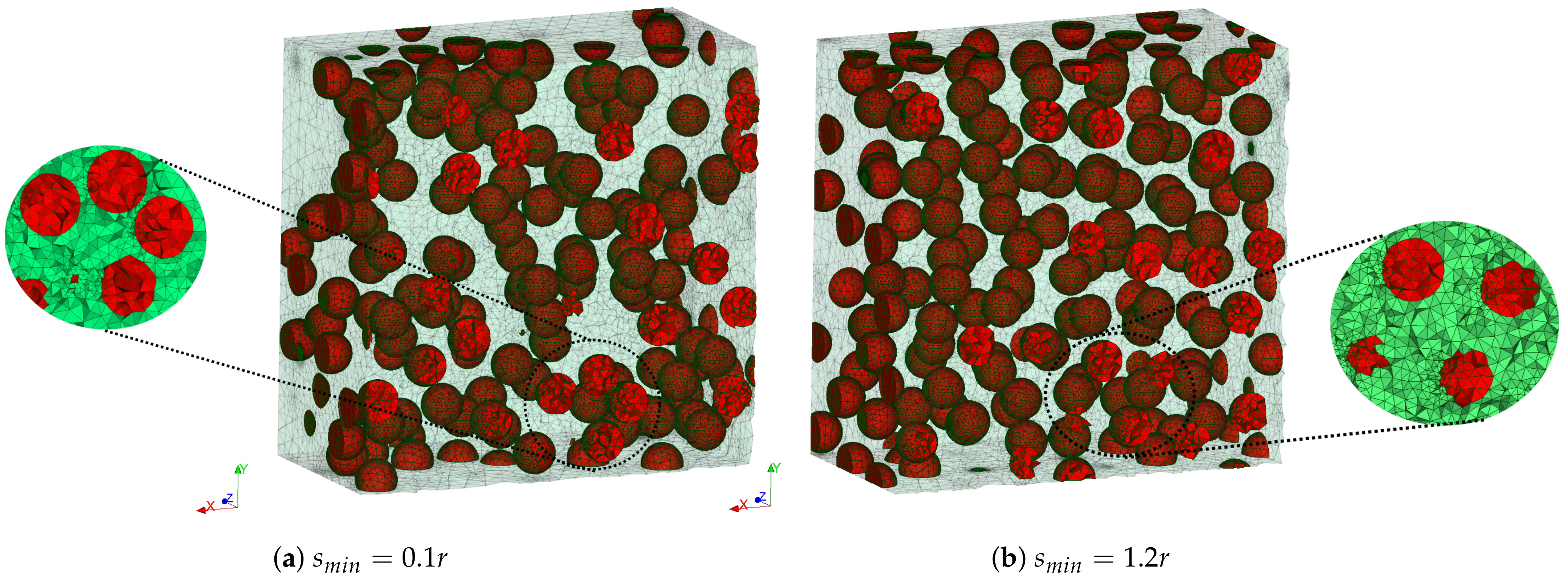
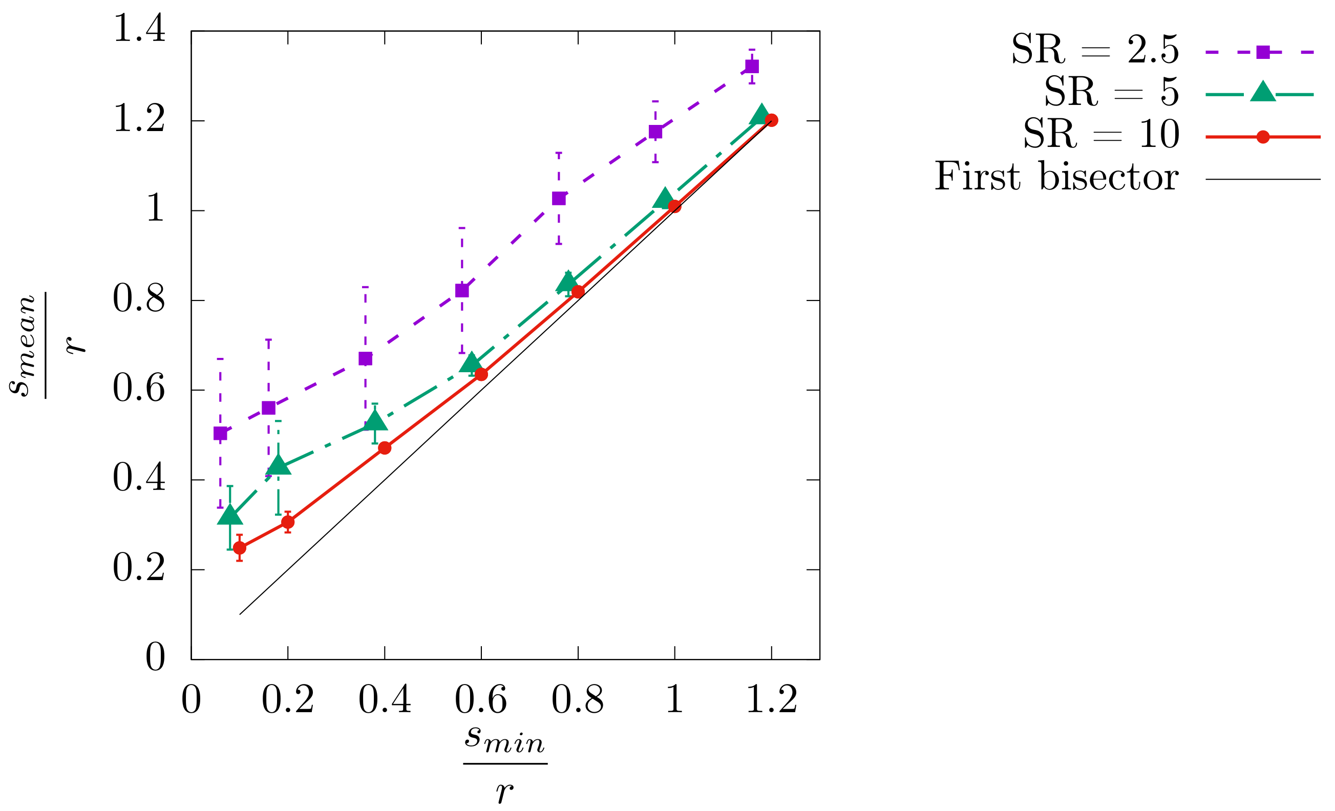
2. Generation of Representative Volume Element of Matrix-Inclusion Composite with an Effective Minimal Distance between Inclusions

This section gives some practical details about the generation of cubic RVE with monodisperse spherical inclusions with an effective minimal distance (in the sense given in the Introduction). For details on the notion of RVE, the reader is referred to [19,20].
Cubic RVE of side l including monodisperse spherical inclusions of radius r are under consideration. The RVE are generated through MEROPE, a software of the PLEIADES platform [21,22] dedicated to simulations on RVE. This software enables us to obtain a simple random sampling of spheres with a mechanical contraction algorithm [23] based on the Random Sequential Addition (RSA) method [24]. A minimum distance between two spheres denoted by s m i n is set. Sampling is rejected if the effective minimum distance is superior to the minimum distance imposed.
The scaling ratio S R is defined by the ratio between the size l of the RVE and the diameter of the inclusions ( S R = l 2 r ). Three scaling ratios S R = 2.5 , 5, and 10 are considered. The number of inclusions is chosen to have exactly the same volume fraction of inclusion f v between the scaling ratios. For each of these ratios, 50, 10, and 5 RVE are generated, respectively, for each value of s m i n depending on f v . Indeed, the maximum value of the packing parameter s m i n r is obtained, considering that each sphere is separated by s m i n :
max ( s m i n r ) = 2 ( C 1 / 3 f v 1 / 3 1 ) , with C as the compactness factor .
In [15], the authors give an upper bound without consideration of compactness. For the considered geometry of the RVE, we use the compactness of the body-centered cubic system C = π 3 8 . At f v = 13.4 %, the maximum value for the packing parameter is then 1.4 and RVE with a minimum (effective) distance between inclusions of s m i n r { 0.1 ; 0.2 ; 0.4 ; 0.6 ; 0.8 ; 1 ; 1.2 } have been generated. Figure 1 shows examples of two RVE with extreme s m i n values at S R = 10 .
The COMBS tool [25] based on the SALOME platform [26] is then used to build periodized RVE from the sphere samples in order to avoid bias in the computation of the effective properties [27]. The finite-element discretization of the RVE is also performed using COMBS. A periodic mesh is then obtained. A previous mesh convergence study [28] showed that quadratic finite elements (rather than linear) have to be used, particularly in terms of stresses obtained in the inclusionary phase. Moreover, thanks to the isoparametric finite-element transformation, quadratic elements lead to a better discretization of spherical shells and then to an accurate mesh approximation of the theoretical (geometric) volume fraction of inclusions f v with much fewer elements [29]. This approximate volume fraction is of first-order importance in the determination of effective behavior (see Section 3). The meshes used in the following process are then composed of ten-node tetrahedral elements.
To guarantee that the mesh is non-degenerated and non-tangled, the minimum number of elements between two boundaries n m i n (between inclusion boundaries or between the inclusion boundary and RVE boundary) is set to 2. This ensures that there is always a node in the matrix between two boundaries. It leads to a non-uniform mesh, with greater mesh refinement between nearby inclusions and in inclusions intersected by boundaries of the RVE (see Figure 1). In practice, the minimum mesh size is dictated by these cut inclusions. Thus, the total number of nodes in the mesh only slightly depends on the minimum distance s m i n . The minimum mesh size is set to r / 200 , whereas the maximum mesh size is chosen to be equal to r. A gradation factor g of 2 is used between elements. These various values were chosen via a preliminary mesh convergence study, the main results of which are shown in Table 1. In this table, the variation in the apparent bulk modulus k a p p (defined in Section 3.3) and its standard deviation with respect to the mesh parameters and number of nodes is reported. We can easily see that this modulus value is converged with the chosen parameter mentioned above. Other more local values show the same convergence in the mesh parameters.
This reliable process of mesh generation, however, leads to a large number of mesh elements. The average value of the number of nodes obtained per S R is presented in Table 2. It can be noted that the variation in the number of nodes is consistent with the scaling ratio.

3. Elastic Properties and Homogenization

3.1. Stiffness Contrasts between Phases

The boundary value problem under consideration is an elastostatic problem, where the composite is subjected to a macroscopic strain E ̲ ̲ . Solving this problem at the microscopic scale consists of determining the fields satisfying the following system of equations in the RVE denoted by V:
d i v σ ̲ ̲ = 0 in V σ ̲ ̲ = C ̲ ̲ ̲ ̲ : ε ̲ ̲ in V ε ̲ ̲ ( u ̲ ) = 1 2 g r a d u ̲ + ( g r a d u ̲ ) T in V B C s on V
where C ̲ ̲ ̲ ̲ is the fourth-order elasticity tensor and the BCs are determined in order to obtain ε ̲ ̲ = E ̲ ̲ (see Section 3.3), where denotes the geometric mean value:
= 1 | V | V d V
with | V | being the measure of V.
Each phase i is supposed to have linear elastic behavior, where index 1 (resp. 2) represents the inclusion (resp. matrix) phase. Isotropic behavior is supposed:
σ ̲ ̲ = E i 1 + ν i ε ̲ ̲ + ν i 1 2 ν i trace ( ε ̲ ̲ ) I d ̲ ̲ in each phase i
with E i being the phase’s Young’s modulus, ν i the phase’s Poisson’s ratio, and I d ̲ ̲ the second-order identity tensor.
The contrast between phases is adjusted by modifying the mechanical parameters of the inclusionary phase for the following digital material:
E 2 = 20 MPa E 1 = E 2 × c o n t r a s t ν 1 = ν 2 = 0.3
By definition, the bulk modulus k = E 3 ( 1 2 ν ) and the shear modulus μ = E 2 ( 1 + ν ) have the same contrast. In this study, soft and rigid inclusions are considered by varying the value of the c o n t r a s t parameter in { 0.01 ; 0.1 ; 10 ; 100 } .

3.2. Analytical Homogenization—Mori–Tanaka Estimates

The Mori–Tanaka (MT) homogenization method is used to estimate the effective properties of the matrix-inclusion materials of moderate volume fractions. The following relationships can be derived (see [5], for example):
k M T = k 2 + f v k 1 k 2 1 + ( 1 f v ) k 1 k 2 4 3 μ 2 + k 2 μ M T = μ 2 + f v μ 1 μ 2 1 + ( 1 f v ) μ 1 μ 2 μ ˜ + μ 2 with μ ˜ = μ 2 6 9 k 2 + 8 μ 2 k 2 + 2 μ 2
Like any analytical estimate, this law has a range of uses. In particular, the volume fraction of inclusions must not be too high [30], typically f v < 40 %. It should be noted that whatever the c o n t r a s t parameter in Equation (5), the Mori–Tanaka estimate (6) returns to one of the Hashin–Shtrikman bounds [31]. The Mori–Tanaka approach also makes it possible to obtain estimates of the phase mean field (first and second moments). This approach is hence often called the “mean-field” approach.
The nth phase moment of a field, denoted by • in a generic way, is recalled in Equation (7):
n i = 1 | V i | V i n d V i
with V i being the domain occupied by the phase i under consideration and | V i | its measure.

3.2.1. The First Moment

By considering the infinite relaxation time in [5], the Mori–Tanaka estimate of the average stress (or stress first moment) in the inclusionary phase is written as
σ ̲ ̲ 1 = 2 μ M T b ˜ d E ̲ ̲ d + 3 k M T b ˜ m E m I d ̲ ̲
where ̲ ̲ d and m denote the deviatoric and spherical part of a tensor, respectively, whereas i denotes the volume average in phase i (cf. Equation (7) applied to σ ̲ ̲ with n = 1 ). We recall that, m = t r a c e ( ̲ ̲ ) / 3 , ̲ ̲ d = ̲ ̲ m I d ̲ ̲ .
The coefficients b ˜ d and b ˜ m of the homogenization tensor required in Equation (8) are given by
b ˜ d = μ 1 μ 2 10 3 μ 2 + 5 2 k 2 3 2 ( 1 f v ) k 2 + ( 3 2 f v + 1 ) μ 1 μ 2 k 2 + 4 3 ( 1 f v ) μ 2 + ( 4 3 f v + 2 ) μ 1
b ˜ m = k 1 4 3 μ 2 + k 2 4 3 μ 2 k ˜ e + k 2 k 1 with k ˜ e = f v k 1 + ( 1 f v ) k 2 .
The average stress in the matrix phase is directly deduced from Equation (8) by considering the relationship
f v σ ̲ ̲ 1 + ( 1 f v ) σ ̲ ̲ 2 = Σ ̲ ̲ ,
where Σ ̲ ̲ is the macroscopic stress on the RVE obtained with the classical formula
Σ ̲ ̲ = 2 μ M T E ̲ ̲ d + 3 k M T E m I d ̲ ̲ .
From the phase mean of the stress tensor, the phase mean hydrostatic (or spherical part) stress can be directly estimated thanks to the MT model:
σ m i = 1 3 trace ( σ ̲ ̲ i ) i = 1 , 2 .
However, the phase mean equivalent (Von Mises) stress cannot be evaluated from the MT estimates due to the nonlinear terms.

3.2.2. The Second Moment

The MT method offers the possibility to directly derive estimates of the second moment of the hydrostatic (spherical part) σ m 2 i and equivalent (Von Mises) stress σ e q 2 i (see Equation (7) applied to σ m and σ e q with n = 2). The equivalent stress (resp. strain) is obtained from the deviatoric part of the stress (resp. strain) tensor:
σ e q = 3 2 σ ̲ ̲ d : σ ̲ ̲ d and ε e q = 2 3 ε ̲ ̲ d : ε ̲ ̲ d E e q = 2 3 E ̲ ̲ d : E ̲ ̲ d .
The second moment of the hydrostatic and equivalent stress is determined from the corresponding strain:
σ m 2 i = 9 k i 2 ε m 2 i , σ e q 2 i = 9 μ i 2 ε e q 2 i
where
ε e q 2 1 = E e q 2 f v μ M T μ 1 , ε e q 2 2 = 1 ( 1 f v ) E e q 2 μ M T μ 2 + 3 E m 2 k M T μ 2 ,
ε m 2 1 = E m 2 f v k M T k 1 , ε m 2 2 = 1 ( 1 f v ) 1 3 E e q 2 μ M T k 2 + E m 2 k M T k 2 ,
with the derivation formulas given in Appendix A.

3.3. Computational Homogenization—Full-Field Simulations

The elastostatic problem (2) is solved with Cast3M [32] on the RVE using the following periodic boundary conditions:
u ̲ ( x ̲ ) = E ̲ ̲ · x ̲ + v ̲ ( x ̲ ) on V ,
with v ̲ being an l-periodic displacement.
For periodic geometries, this type of condition exhibits better accuracy and convergence in the scaling ratio [19,33]. As all the local information is immediately accessible through this approach, it is commonly named the “full-field approach”.
Whatever the microstructure, it is possible to obtain the whole effective (homogeneous) elasticity tensor from computations (and then stress average) in the RVE with unit loadings (6 in 3D) in macroscopic strain E ̲ ̲ . In the case studied here, the effective behavior of the material is isotropic due to the geometry of the RVE and the sampling (spherical inclusions randomly distributed in a periodic cubic volume). Thanks to this isotropic form of the effective elasticity tensor, it is possible to derive the apparent effective properties via the compressibility modulus k a p p and the shear modulus μ a p p , with fewer but well-chosen loadings. Although in [19] two loadings are considered, we show here that a single mixed loading is sufficient (see Equation (19)).
E ̲ ̲ = 1 . 1 . 0 . 1 . 0 . 0 . 0 . 0 . 0 . k a p p = 1 3 trace ( Σ ̲ ̲ a p p ) μ a p p = 1 4 ( 3 2 Σ X X a p p 1 2 trace ( Σ ̲ ̲ a p p ) + Σ X Y a p p ) ,
with
Σ ̲ ̲ a p p = σ ̲ ̲ .
It can be noted that more terms than are used in [19] are also used for the calculation of μ a p p , which ensures the better stability of this value.
The phase mean fields (corresponding to the first and second moments) are obtained directly from the local stress field (see Equation (7)).

4. Numerical Results

The RVE described in Section 2 are used to study the effects of inclusion proximity on the composite behavior. Unless otherwise specified, inclusions are assumed to have a radius r = 10 μ m and a volume fraction f v = 13.4 %. The mean value and standard deviation on the mean value over the samples are determined for all quantities of interest. In order to appreciate and compare the global trends, these numerical post-treatments are normalized by the corresponding computational mean value obtained from calculations on the RVE with the maximum S R (generally S R = 10 is considered as the reference due to the low result dispersion) and the maximum s m i n (configurations where the inclusions are the most equally distributed in the matrix). These normalization values are marked by an overline symbol ¯ .
The discussion focuses on stiffness c o n t r a s t s of 0.01 and 100 between phases (cf. Equation (5)), as similar tendencies are observed for c o n t r a s t s of 0.1 and 10, respectively. For the sake of completeness, the results for the latter contrasts are reported in Appendix B (effective properties), Appendix C (phase mean field), and Appendix D (local stress field).

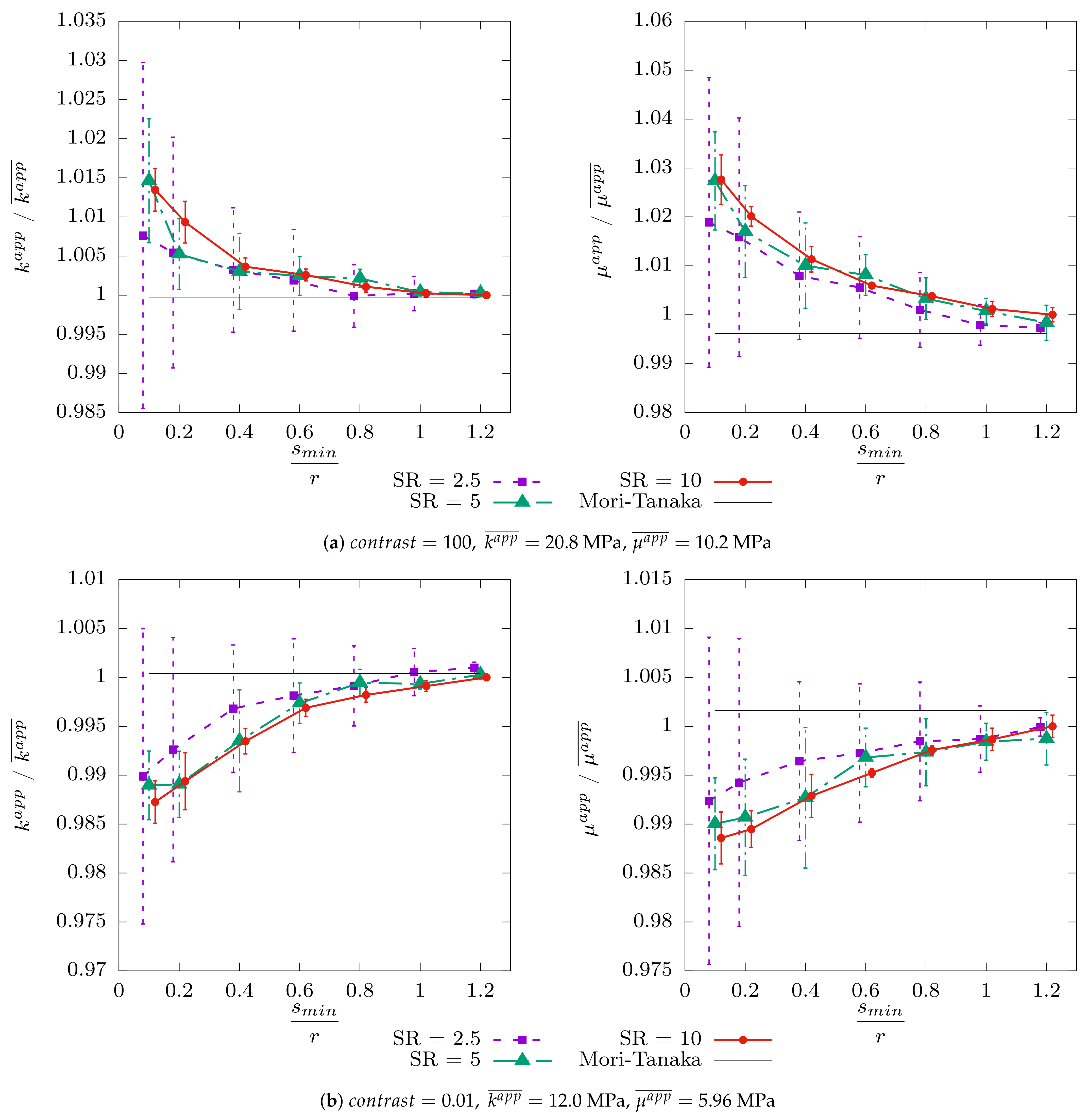
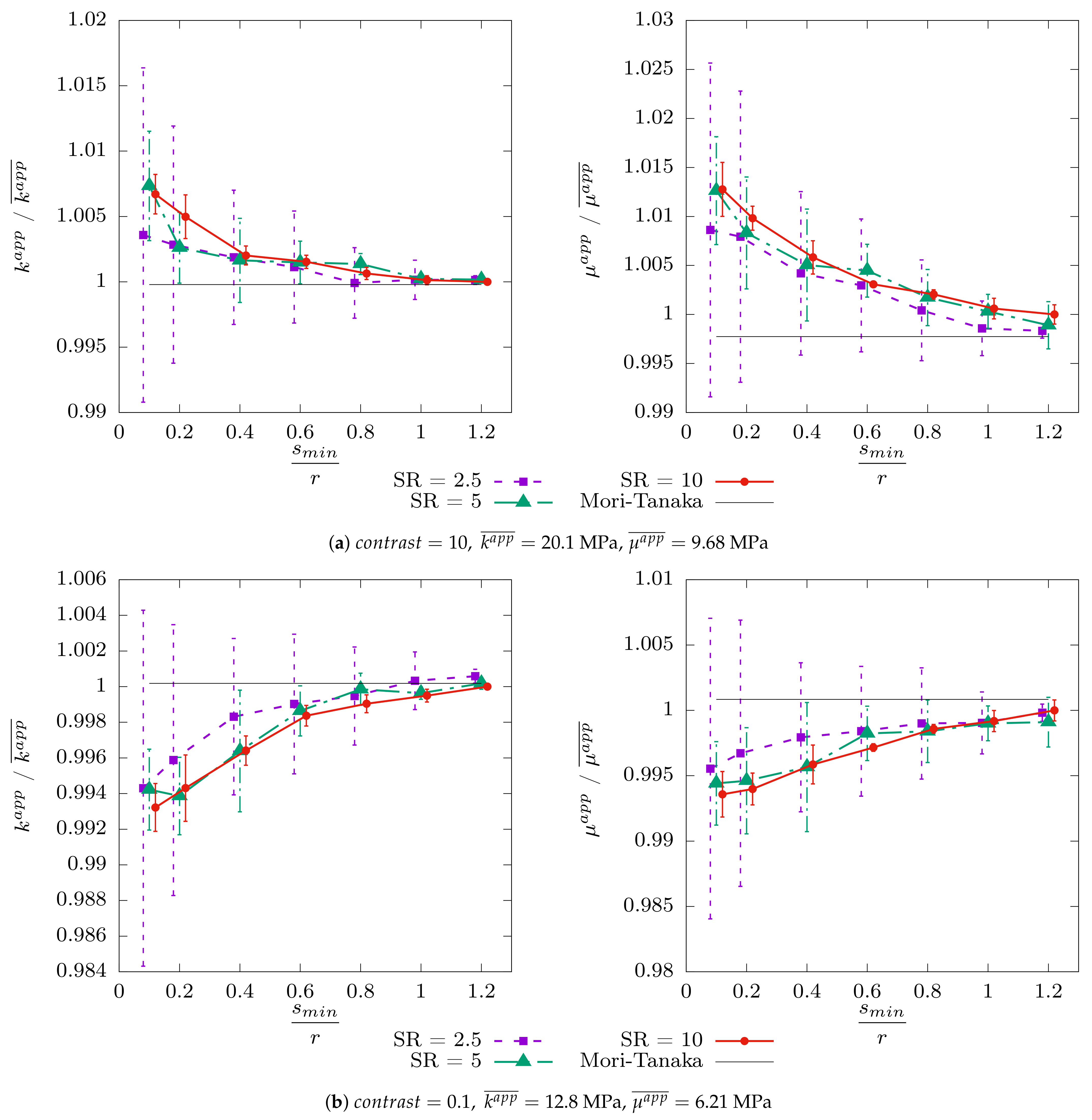
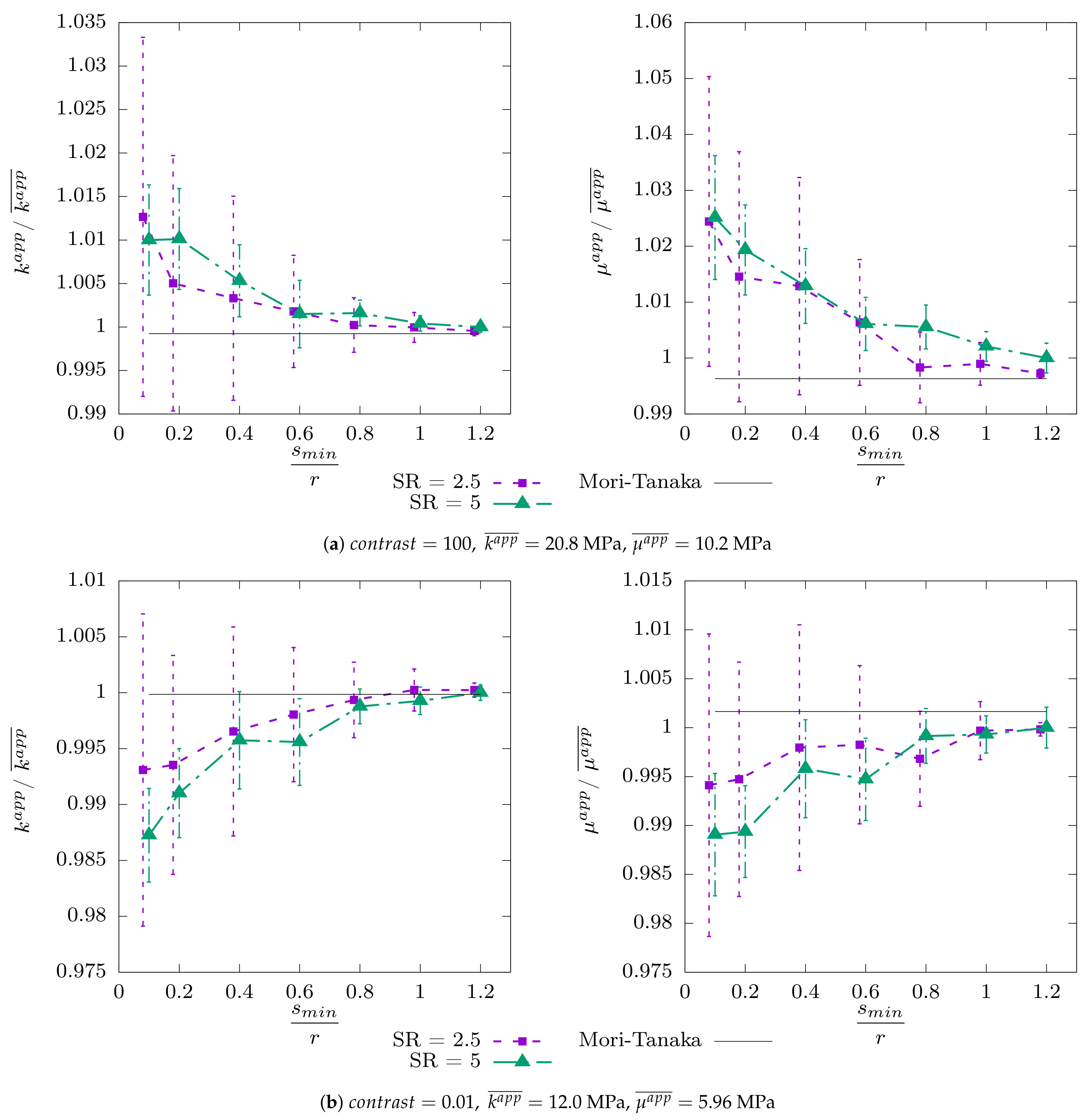
4.1. Results for the Effective Properties

In this section, the apparent moduli (bulk modulus k a p p and shear modulus μ a p p ) obtained through the full-field simulations (see Equation (19)) are compared to the Mori–Tanaka estimates (see Equation (6)).
The influence of the effective minimum distance s m i n on the effective properties is reported in Figure 2.
The first conclusion that can be drawn is that the mean values vary slightly between different S R s. As expected, when the scaling ratio increases, the standard deviation decreases to become very low at S R = 10 . We also note that, whatever the S R , the standard deviation decreases as s m i n increases, becoming almost negligible at s m i n = 1.2 r . This tendency is due to a kind of bias of the samples at a high s m i n . Indeed, the possibility of distributing the inclusions decreases as s m i n increases. Considering the periodicity, very similar RVE are obtained and, therefore, the numerical results remain close between the samples. This can be confirmed by Figure 3, which shows the mean distance between spheres s m e a n as a function of the effective minimum distance s m i n for the different scaling ratios. As expected, the standard deviation of s m e a n decreases as s m i n increases and becomes almost zero at s m i n = 1.2 r for scaling ratios higher than 5. Moreover, it appears that the curves converge asymptotically to the first bisector s m e a n s m i n as s m i n increases. The higher the scaling ratio, the faster the speed of convergence. Fluctuations of the average at S R = 5 denote a lack of samples for this ratio.
Concerning the proximity effect on the effective properties, we note in Figure 2, a stiffening (resp. softening) of the material when the inclusions are becoming closer for rigid (resp. soft) heterogeneities. We should underline that numerical computations confirm that the Mori–Tanaka estimates are a Hashin–Shtrikman bound (low or high depending on the contrast between phases). The effect of the distance between inclusions seems to vanish when this distance becomes greater than the sphere radius. This result is in good agreement with the distance of influence of the inclusions on the matrix mentioned in [34]. The effective properties tend toward an asymptote whose value is well predicted by the Mori–Tanaka estimate. This is consistent with the theoretical assumption of inclusions seeing only the matrix around, on which these estimates are built. Quantitatively speaking, for this very moderate volume fraction ( f v = 13.4 %), the deviation only reaches a few percent for low minimum distances between inclusions.
For the sake of completeness, the influence of the sphere radius and volume fraction of inclusion has been studied. For both cases, simulations at S R = 10 were not performed since the results obtained at S R = 5 were accurate enough to check for a trend (see Figure 2). This shows that the sphere radius size (for a given volume fraction) has neither a qualitative nor a quantitative effect on the observed behaviors with respect to the packing parameter s m i n / r (see Figure A2 in Appendix B for r = 5 μ m). On the contrary, the volume fraction of inclusion exacerbates the deviation of the effective properties with a decreasing s m i n / r (see Figure 4 for f v = 25.1 % with r = 10 μ m, as in Figure 2) but with m a x ( s m i n / r ) = 0.8 (see Equation (1)). In this case, the difference can reach around 10 % on the effective shear modulus for rigid inclusion. The effective properties’ deviations with the packing parameter hence appear to be proportional to the volume fraction of inclusions. These results are in good agreement with the observations in [14]. By increasing the volume fraction, the convergence of s m e a n to s m i n is faster and more close spheres contribute to stiffening/softening the material.
A tendency to soften the effective properties for porous inclusions ( c o n t r a s t < 1 ) was also recently observed in [35] in the case of microstructures with cylindrical channels between the pores of a spherical shape. The authors showed that the effective properties are smaller (even for a low volume fraction of channels) than those obtained with a microstructure without channels but with the same total volume fraction. In Section 4.3, we show that the perturbation zone between the close inclusions can indeed be assimilated to channels, or, more generally, to a network, between inclusions.
Concerning the behavior as a function of s m i n / r , in the case of rigid inclusions ( c o n t r a s t > 1 ), the authors of [14] drew similar conclusions in relation to material stiffening when s m e a n / r (precisely s m e a n / 2 r in their article) decreases.
Given the possibly marked deviation between the analytical estimates and the computational homogenized values, an analytical approach considering the packing effect within the RVE would be interesting. With regard to the application of the MRP approach conducted in [14], by taking into account the mean distance between spheres s m e a n / 2 r but leading only to a qualitative (and not quantitative) prediction of the effective behavior, Figure 3 may indicate that it is better to focus on the relative minimum distance s m i n / r between inclusions.

4.2. Results for Phase Mean Fields

One of the novelties of this contribution is studying the effect of the inclusion proximity on the (volume) phase mean fields. As the Mori–Tanaka approach enables us to obtain estimates for such kinds of quantities of interest (see Section 3.2), a comparison of the analytical and computation mean stresses can be performed. The first and second moments of hydrostatic and equivalent stresses by phase are analyzed hereafter.

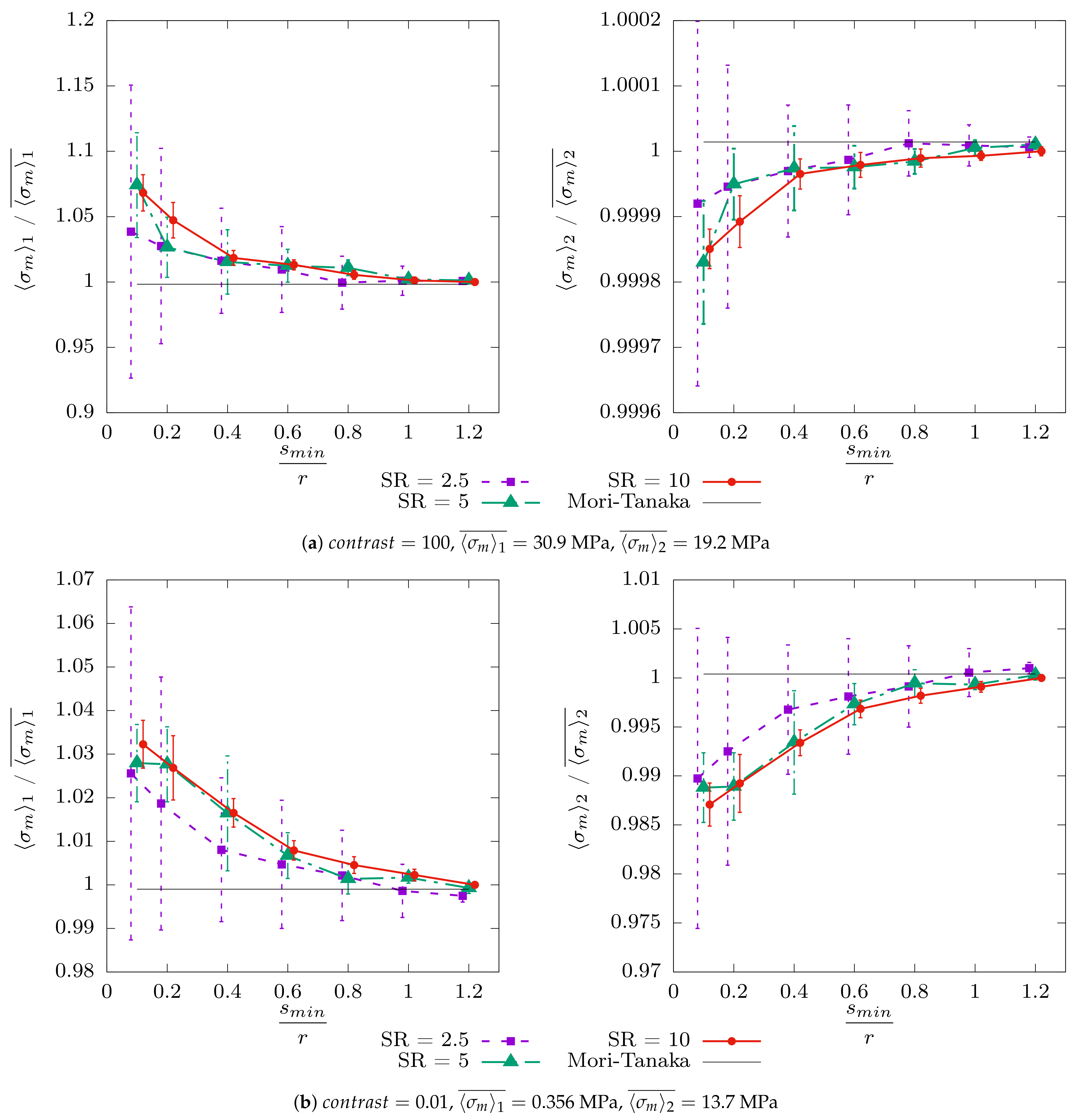
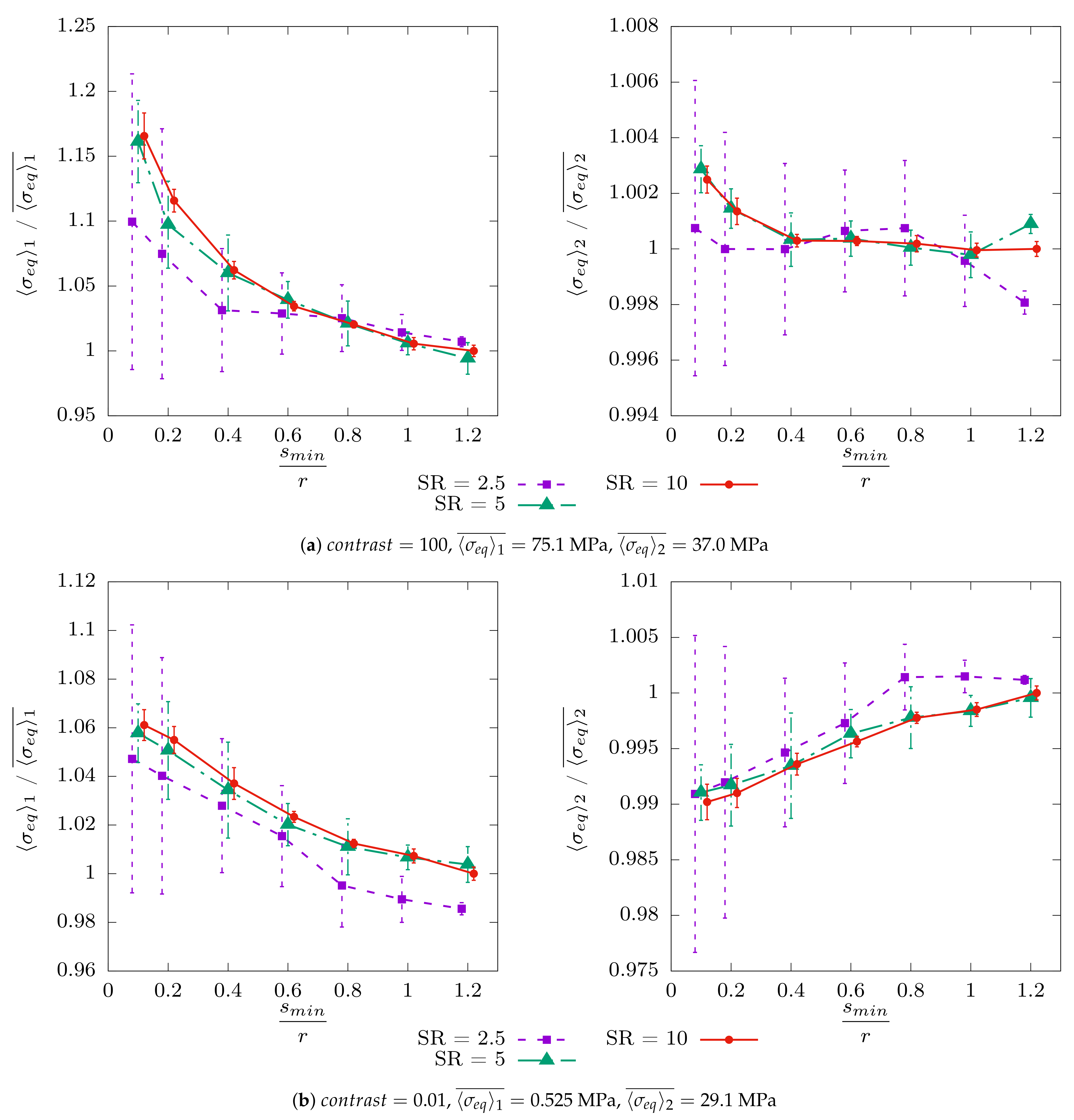
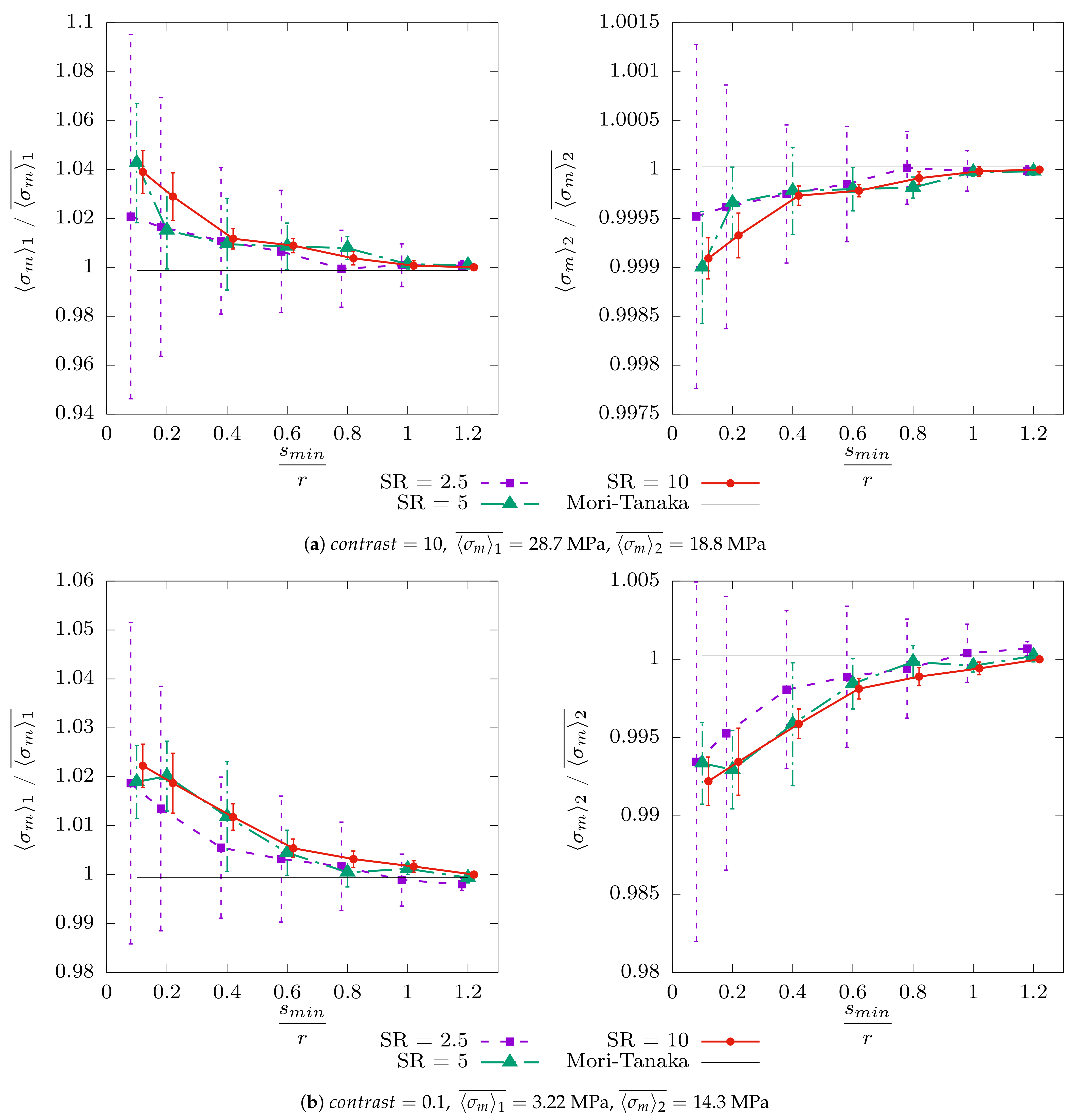
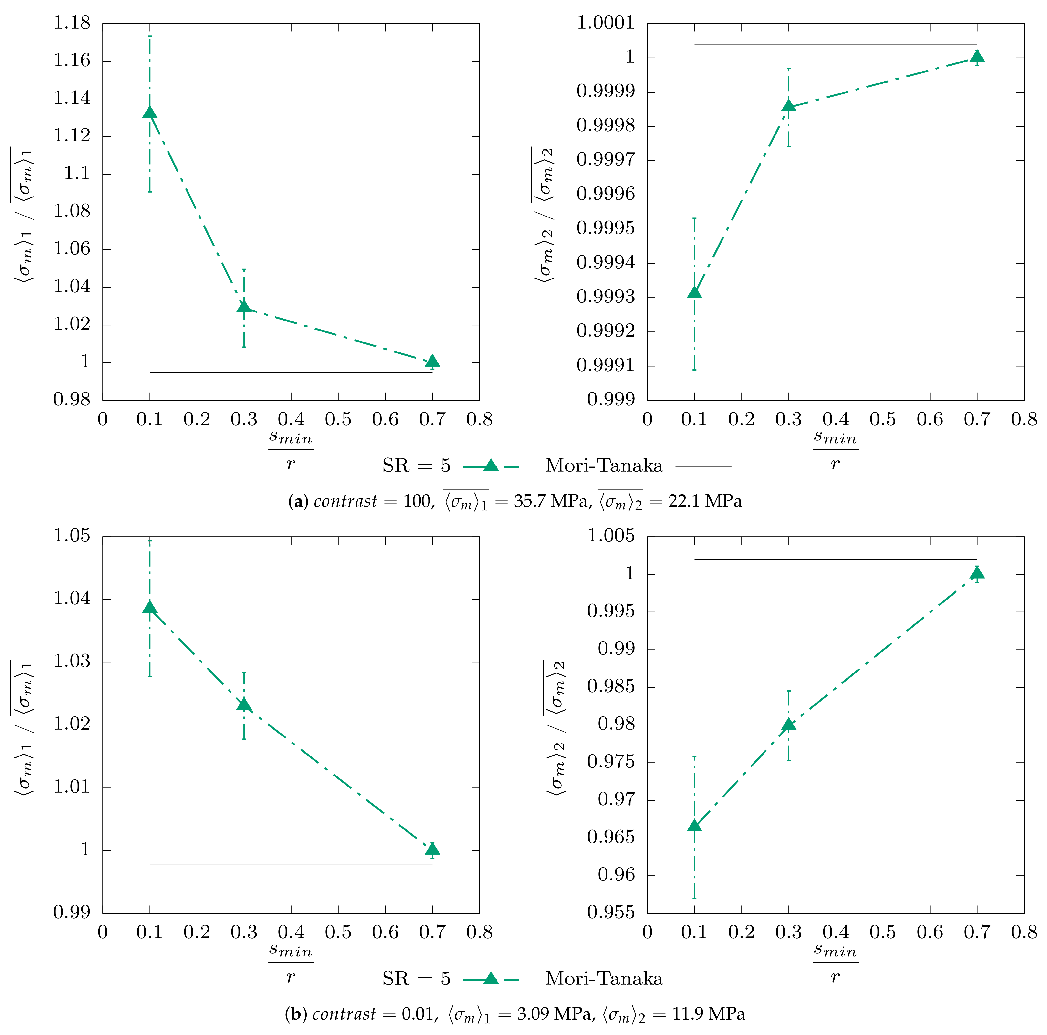
4.2.1. The First Moment

Hydrostatic Stress
In Figure 5, the evolution of the phase first moment of hydrostatic stress (namely σ m i , i = 1 , 2 ) is plotted as a function of s m i n / r for different contrasts and scale ratios.
First, identical conclusions to those in Section 4.1 can be drawn on the weak influence of the S R on the trend in the results on average. On the other hand, we observe here that the shape of the curves does not depend on the contrast. When the spheres come closer together, the mean hydrostatic stress tends to increase (resp. decrease) in the inclusionary (resp. matrix) phase, regardless of the contrast between the phases. We see that the rigid phase dictates the effective properties, with curves very similar to those of the effective properties plotted in Figure 2.
For rigid inclusions, the mean hydrostatic stress in the inclusionary phase is most impacted by the closeness of the inclusions, the matrix having globally a more stable average behavior (deviations < 1 %). In this case, the deviation of the inclusion means that the stress can exceed 10 % (see Figure A4 for f v = 25 %). Similarities can be found with [36], where the influence of the shape of rigid inclusions (polyhedra and spheres) on the phase mean field was studied. They observed that the mean stress in the inclusionary (resp. matrix) phase in the case of polyhedra was higher (resp. lower) than that in the case of spheres. The behavior of nearby spherical inclusions ( s m i n < 0.5 r ) studied here is similar to that of polyhedral inclusions, which seems geometrically consistent.
For soft inclusions, the inclusionary phase is less impacted and has a moderate deviation. The matrix is more impacted than that of rigid inclusions. A deviation of the same order of magnitude is observed for the matrix and the inclusions.
Equivalent Stress
Figure 6 shows the evolution of the phase first moment of the equivalent stress (namely σ e q i , i = 1 , 2 ) as a function of s m i n / r for different contrasts and scale ratios. As previously underlined in Section 3.2, no MT estimates can be deduced for this quantity.
Globally speaking, the results are close to those obtained for the hydrostatic stress. However, the values of the deviation at the minimum s m i n / r , especially for the inclusionary phase, are doubled and can reach more than a 15 % difference. We can see that for (very) rigid inclusions, the tendency looks different for the matrix phase. For example, for c o n t r a s t = 100 , the equivalent stress decreases as the inclusions become further away. It can be supposed that as the contrast increases, the influence of the shear stress becomes locally important. It should be noted that these conclusions are in good agreement with the results of [36], considering the same analogy as previously (i.e., low s m i n / r → polyhedral inclusions, large s m i n / r → spherical inclusions): the hydrostatic stress in the matrix is greater with spherical inclusions than with polyhedral ones, whereas the equivalent stress is lower for the same comparison.

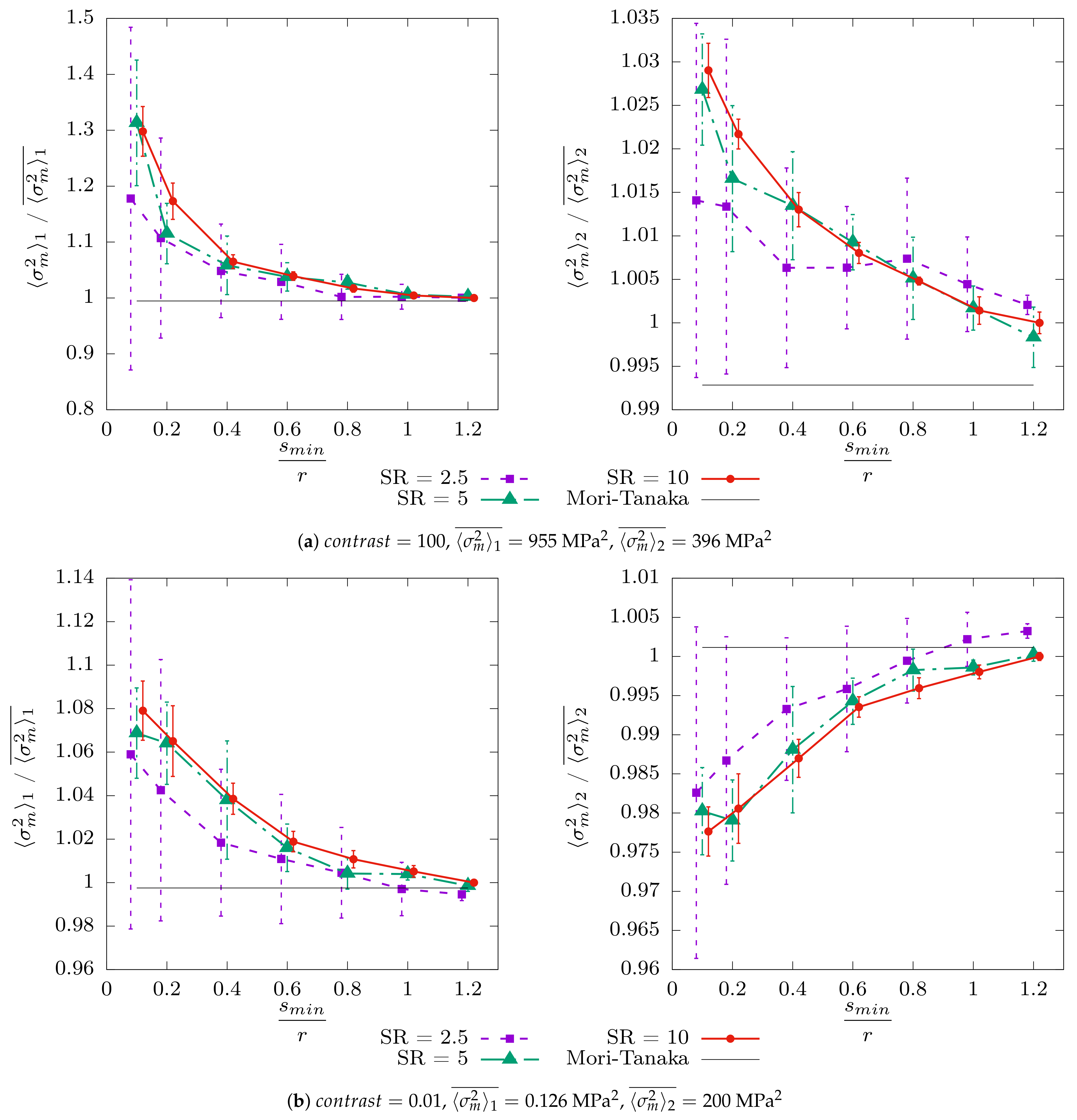
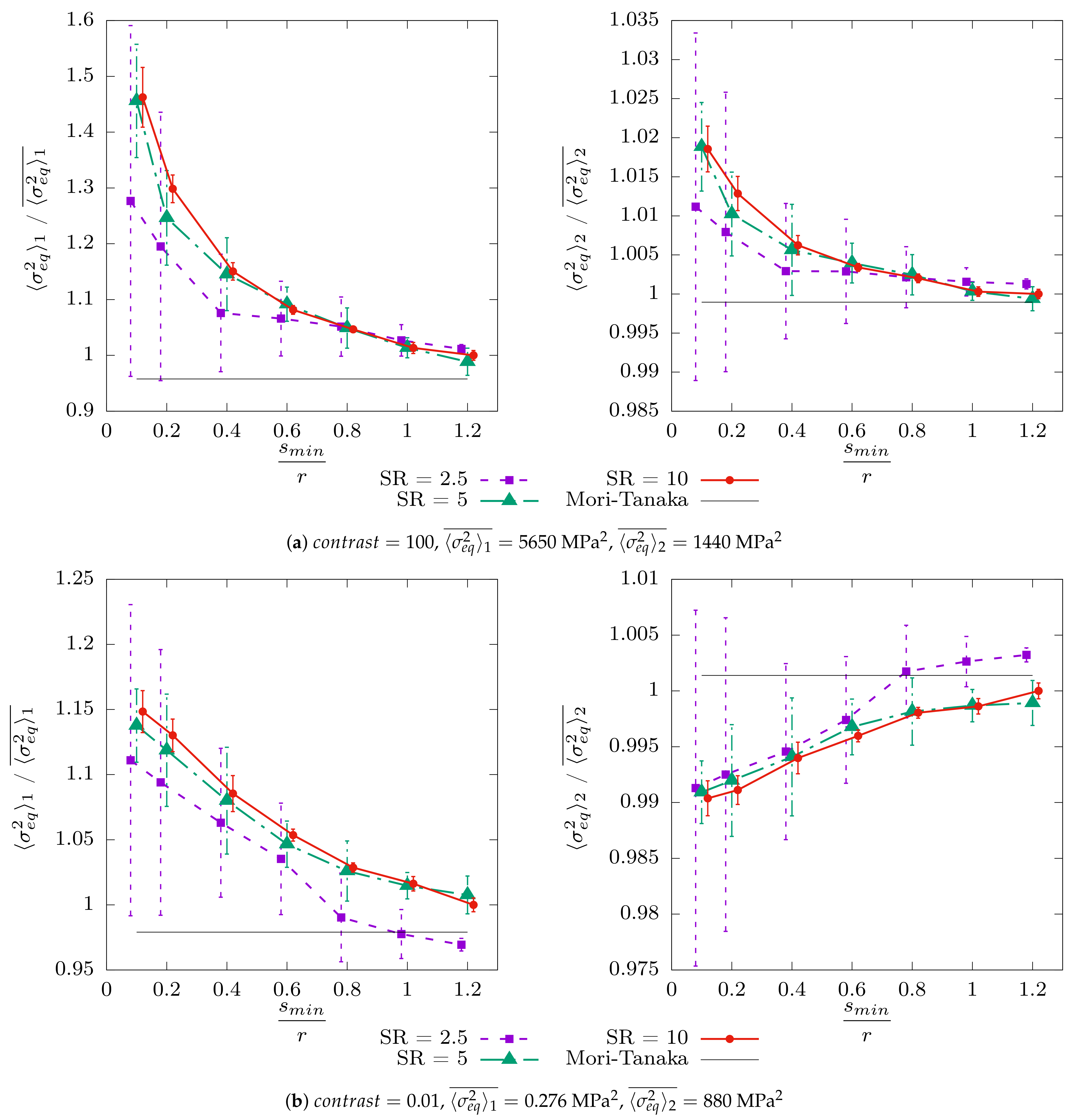
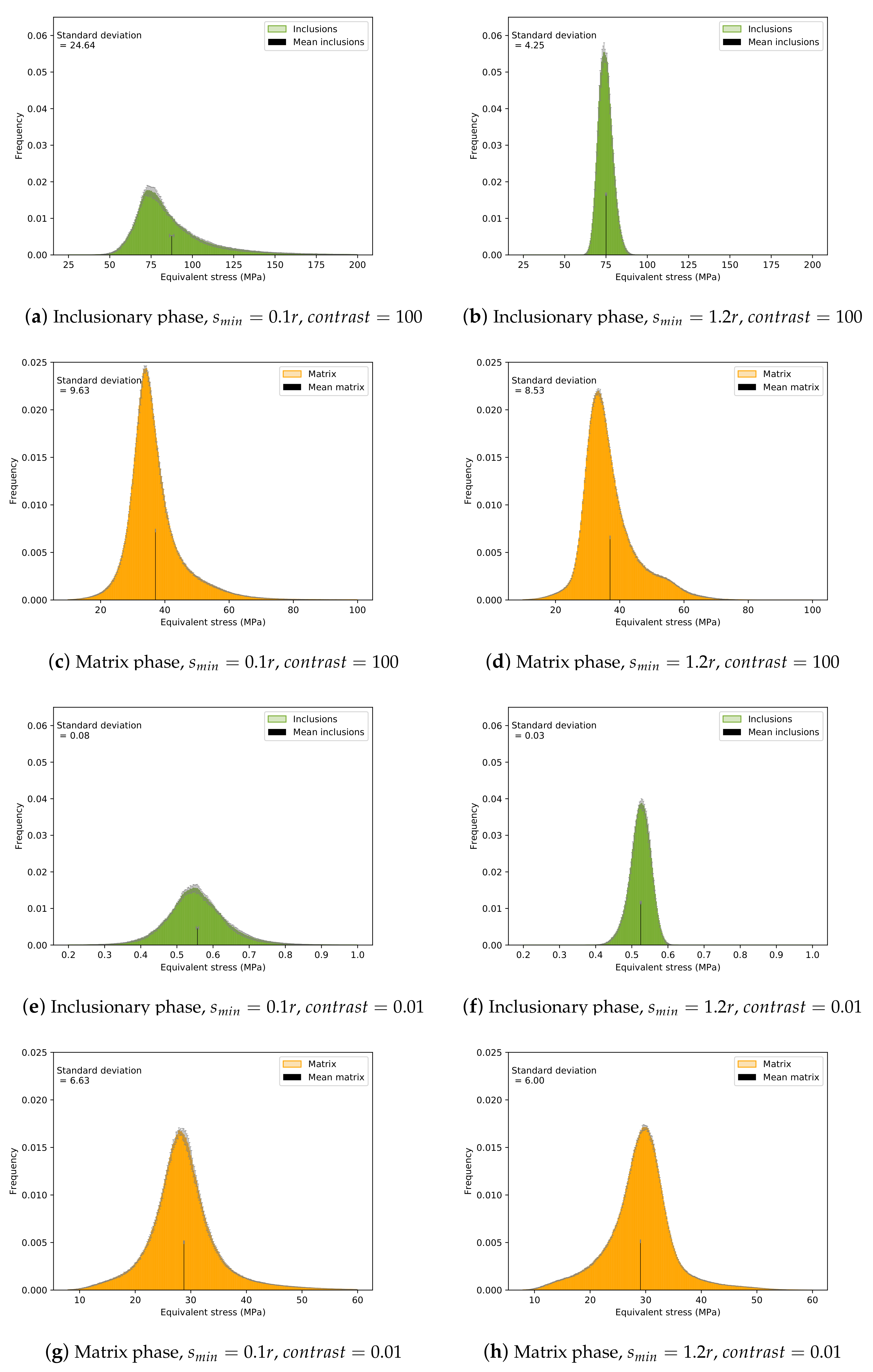
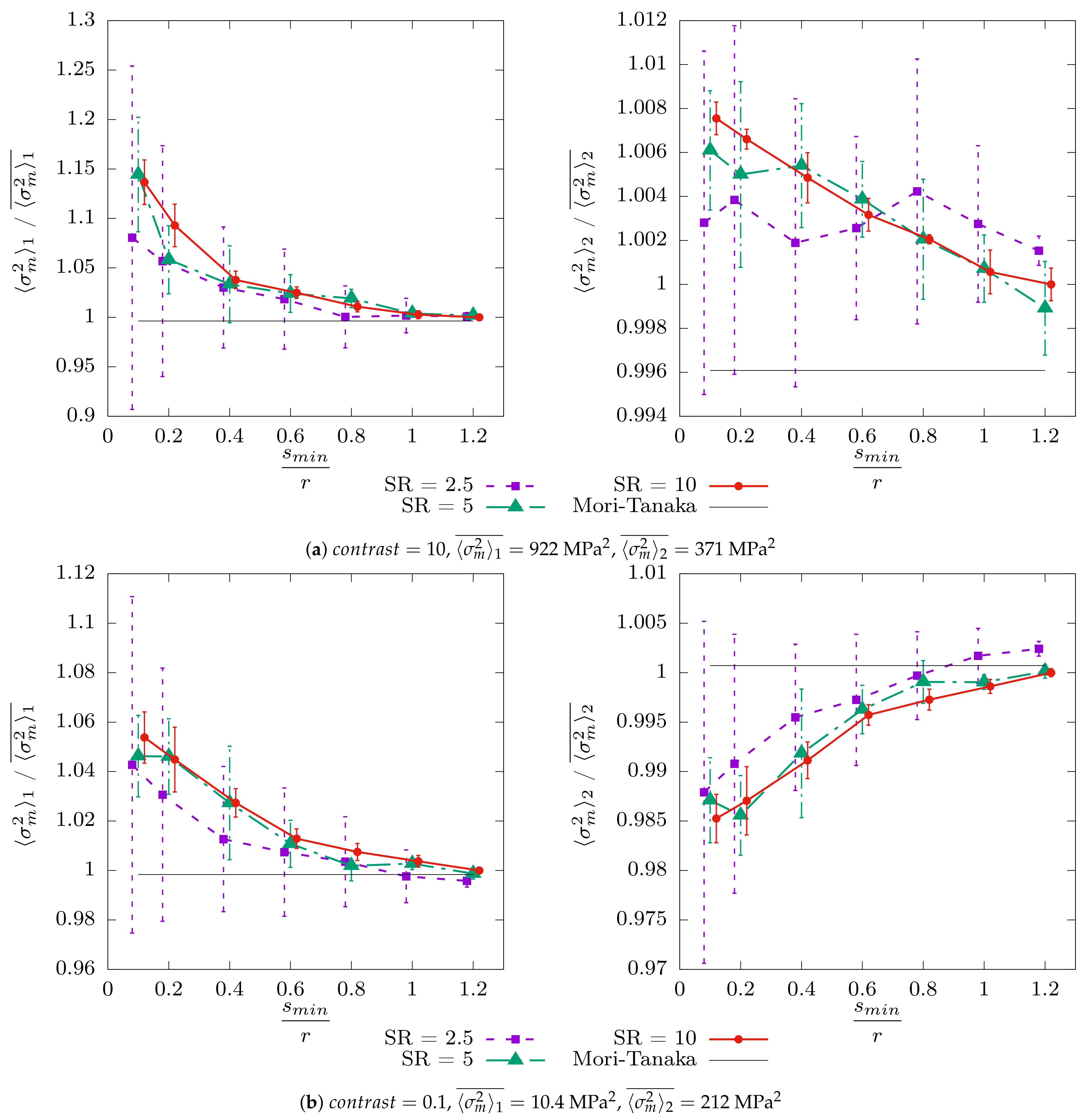
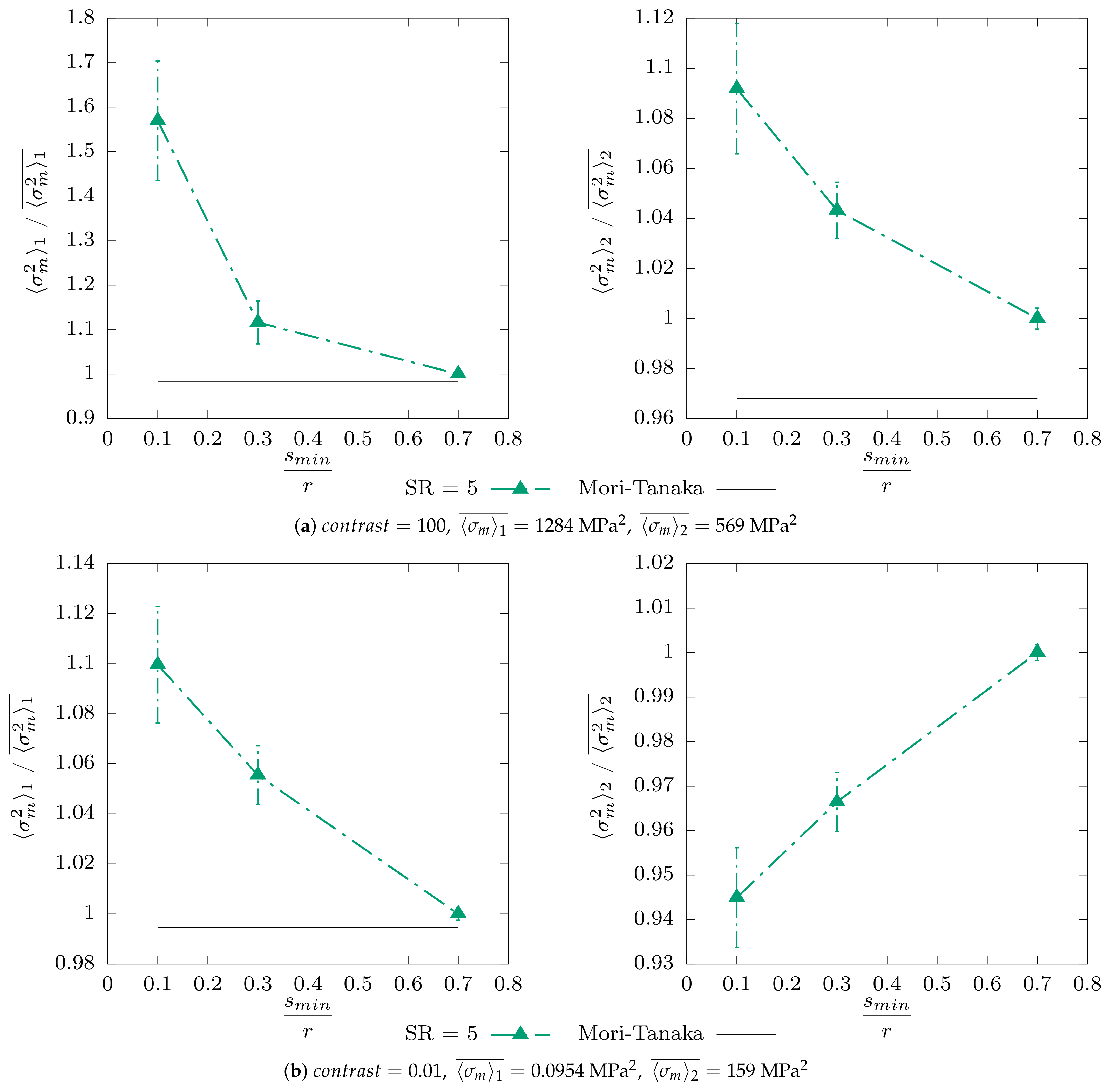
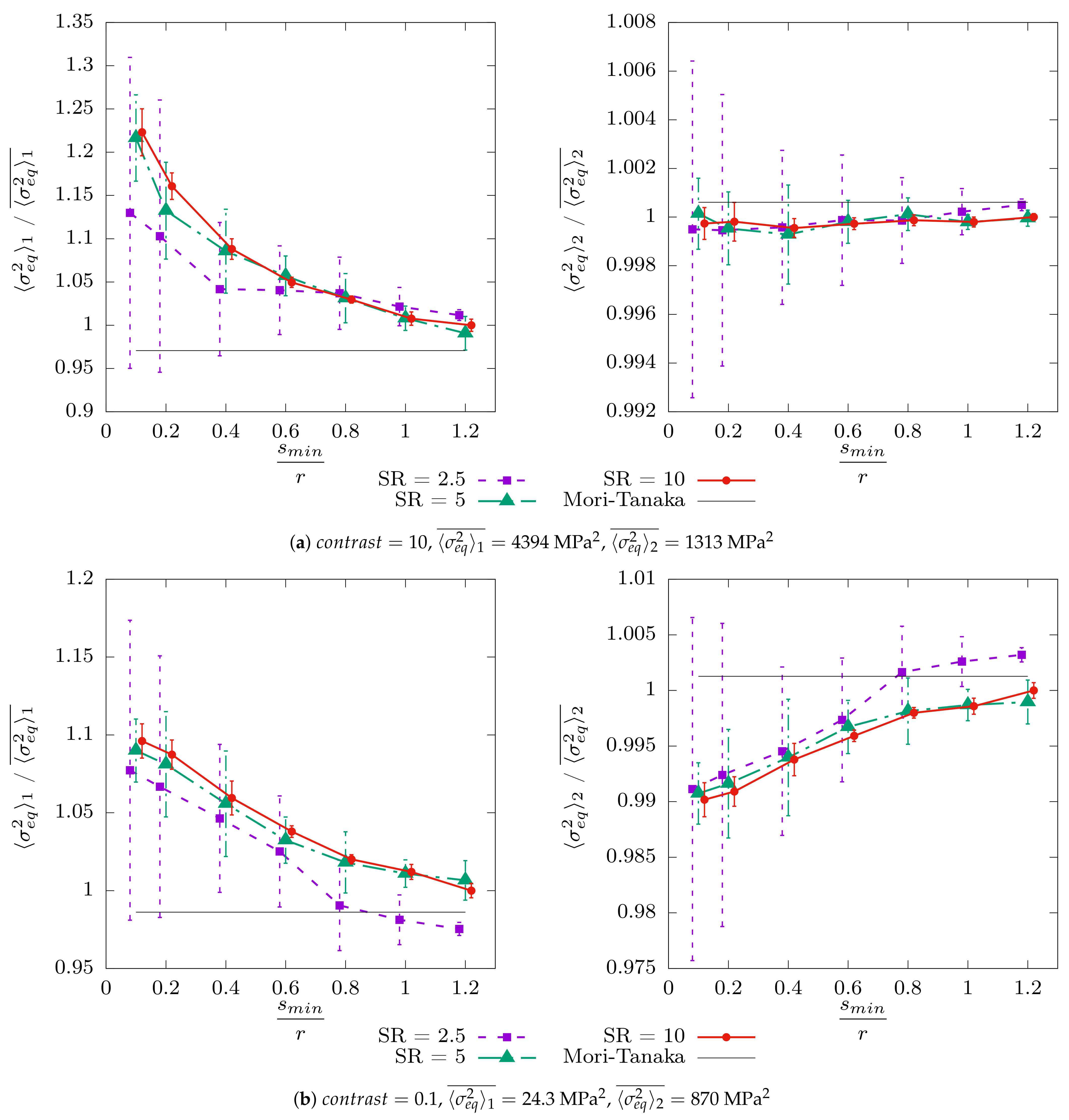
4.2.2. The Second Moment

The evolution of the second moment of hydrostatic and equivalent stresses by phase ( σ m 2 i and σ e q 2 i , respectively) with respect to the distance parameter s m i n / r are plotted in Figure 7 and Figure 8, respectively.
The trends observed are similar for both types of stresses. To understand them, it is useful to consider the following definition of the second moment:
2 i = V i ( ) + i 2 ,
with V i being the variance (square of the standard deviation) in phase i = 1 , 2 .
In the inclusionary phase, the standard deviation varies with the packing parameter in the same way as the first moments. Indeed, the stress tensor tends to be homogeneous (low standard deviation) when the inclusions are far apart but very perturbed (high standard deviation) when the inclusions are close. These observations are confirmed by the analysis of local fields in Section 4.3. As a result, the second moments tend to increase when s m i n / r decreases. The differences are exacerbated compared to the first moments, as the deviation can reach 30 % (hydrostatic stress) or 50 % (equivalent stress) for the rigid inclusions that are the most impacted. The deviation reaches around 10 % for soft inclusions.
For the matrix phase, there is clearly a different tendency whether the inclusions are soft or rigid. For rigid inclusions, the second moment increases when the inclusions become closer, whereas the opposite behavior is observed for soft inclusions. As the first moments are almost constant for rigid inclusions, the observed behavior returns to that of the standard deviation in the matrix. For soft inclusions, the standard deviation varies less with respect to the packing parameter; thus, the behavior roughly remains coherent with that of the first moments. In any case, the deviation remains reasonable in the matrix, with a maximum value of 3 %. However, this deviation becomes more important with higher volume fractions of inclusion. For example, for f v = 25.1 %, the difference in the second moment of the hydrostatic stress in the matrix can reach 10 % (see Figure A7).
Concerning the comparison with the MT estimates, we still observe a well-marked asymptotic convergence of the computational values to the MT estimates when s m i n / r increases. In the inclusionary phase, the deviations are far too large to consider MT a good estimator when s m i n / r < 0.5 . Hence, thanks to Equation (1), correct estimations thanks to the MT approach cannot be obtained for volume fractions of inclusion greater than 35 %. This maximal volume fraction is in good agreement with what is stated in the literature (see, for example, [30]).

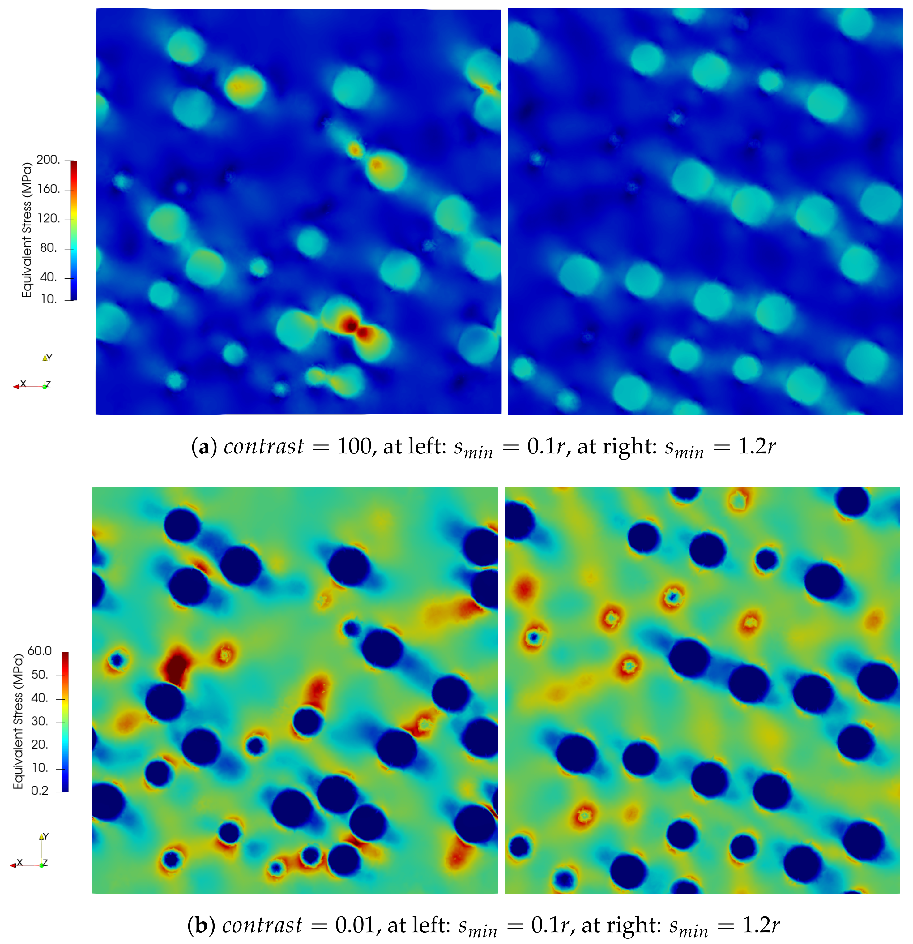
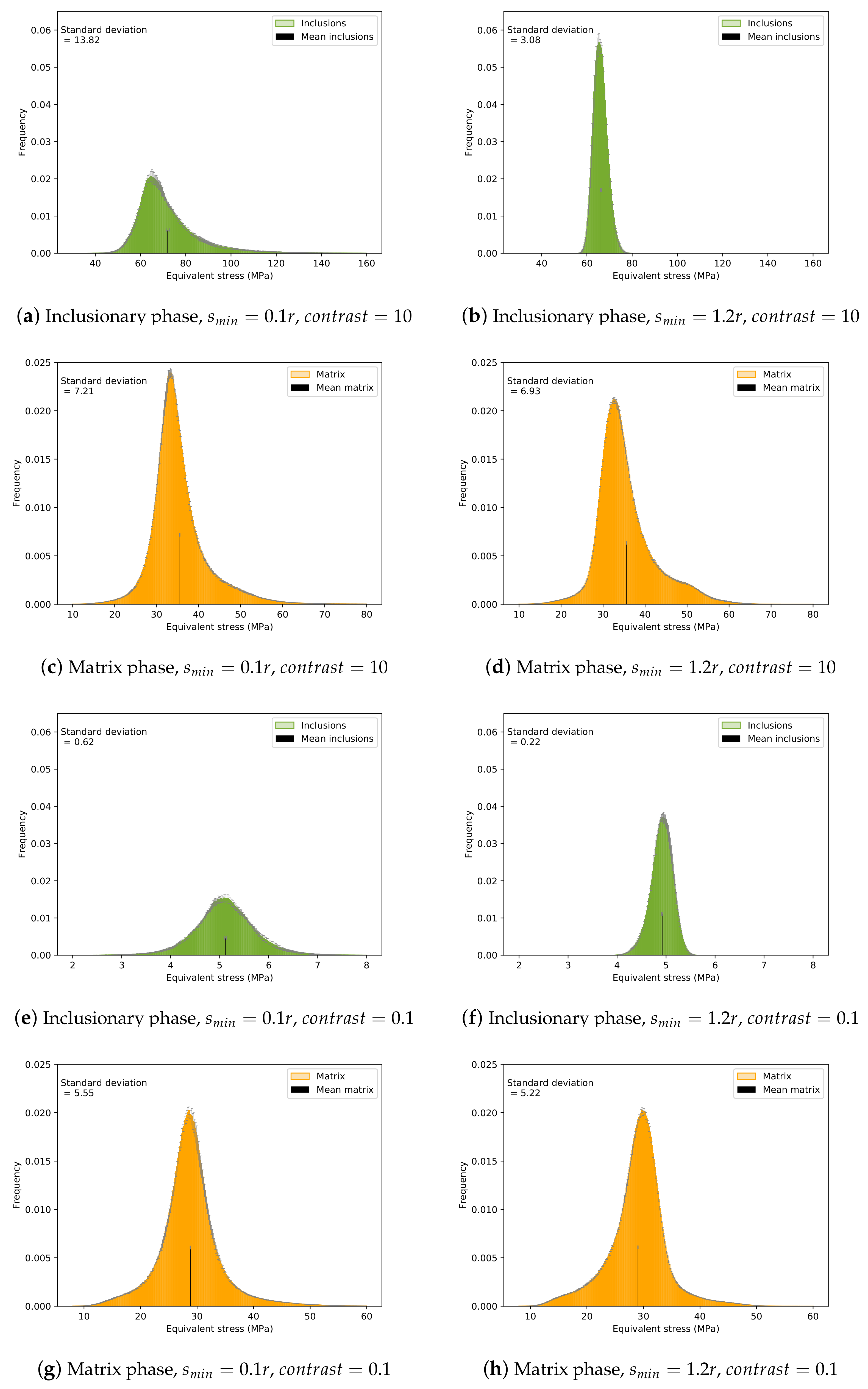
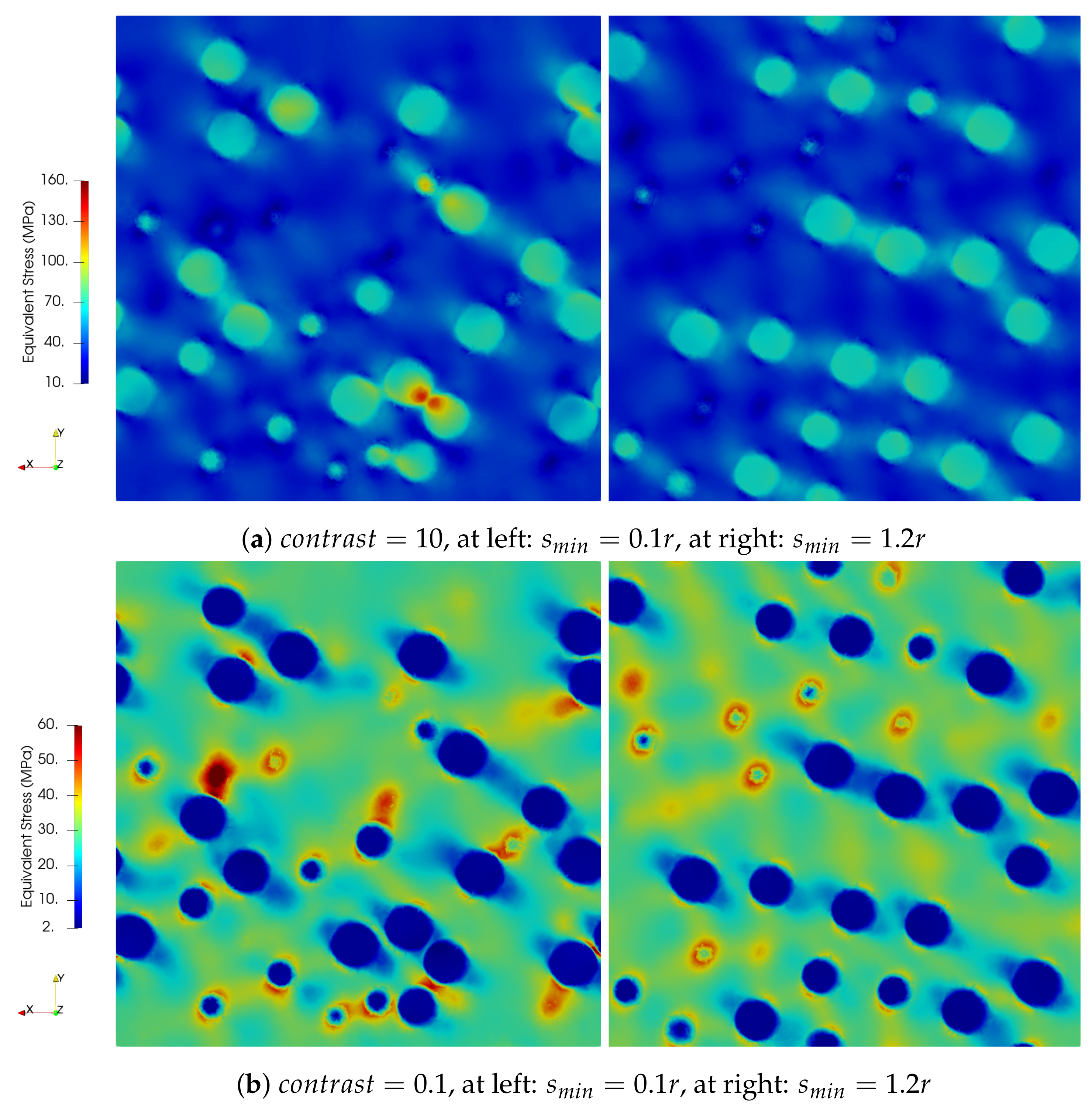
4.3. Results for the Local Fields

Frequency histograms of the equivalent stress within each phase are plotted in Figure 9 for extreme minimum distances ( s m i n = 0.1 r and s m i n = 1.2 r ). The first conclusion that can be drawn is that the further apart the inclusions, the more homogeneous the behavior within them. This is in good agreement with the uniform solution of a single inclusion in an infinite matrix [17]. The inclusionary phase is clearly the most impacted by the variation in the packing parameter s m i n / r . The standard deviation can be up to 5 times larger. Globally speaking, the matrix is slightly affected by the proximity of inclusions. However, we can observe at s m i n / r = 1.2 (cf. Figure 9d) a second little peak that does not appear at s m i n / r = 0.1 . This peak is also mentioned in [36] and explained by the authors by a concentric matrix region of high equivalent stress surrounding each spherical inclusion. We have already noticed this disturbance in the matrix by the inclusions in Section 4.1, which is consistent with the work of [34]. The authors of [36] observed that this peak is less pronounced with polyhedral inclusions than with spherical inclusions, which is consistent with our results, considering the same analogy as in Section 4.2: the behavior of nearby spherical inclusions is similar to that of polyhedral inclusions. In fact, we can observe that the stress values at s m i n = 0.1 r are higher and hence move further to the right of the histogram. Indeed, the histogram is wider (cf. Figure 9c).
These localized effects are not sufficiently visible on the histograms as they only concern a very small region of the microstructure. Thus, the cross-sectional views of the RVE at S R = 10 are presented in Figure 10 for the extreme s m i n . For the sake of comparison, the same scale has been used for each contrast. Figure 10a confirms that the higher stress values are located in the disturbance area of the matrix between two close inclusions. We can clearly see that the matrix perturbation zones near an inclusion/matrix interface are of the order of the radius of the spheres (cf. [34]), as already mentioned in Section 4.1. In agreement with the observations made in [36], this perturbation zone clearly follows the load direction (see Equation (19)). These stress values can be twice as important as those between distant inclusions. These exacerbated perturbation phenomena between close inclusions are less marked when the inclusions are soft, which is in good agreement with all our previous conclusions.
Moreover, when the inclusions are close, a network clearly appears between the spheres, which corroborates our parallel with the channel network (cf. [35]). Finally, by looking at the closest spheres, the parallel with a polyhedral shape of inclusions (cf. [36]) is more easily understood.

5. Conclusions

The proximity effect of moderately dilute monodisperse spherical inclusions in a matrix-inclusion composite has been studied in this paper. Beyond the effective properties, we analyze the behavior of the stress moments (first and second) per phase and the local full fields, which have been never before been performed in the literature. Comparisons with the widely used Mori–Tanaka estimates are also proposed, which is of great interest, especially for the phase first and second moments.
A stiffening (resp. softening) of the composite for the rigid (resp. soft) heterogeneities is observed when inclusions become closer, in particular, at a distance below the radius of the spheres. However, the deviation of the effective moduli remains acceptable (less than 5 %) and the Mori–Tanaka estimates are shown to be reliable.
The effect of the packing parameter, proven to be s m i n / r with s m i n the minimal effective distance between spheres in the sampling and r the sphere radius, appears more important on the phase moments, especially in the inclusion phase (minority phase). For the second moment, the deviation can reach 50 %. It is shown that the Mori–Tanaka estimates are valid for a packing parameter of s m i n / r > 0.5 , which is in good agreement with the assumption of isolated inclusions behind this analytical approach. These conclusions can be extrapolated to the case of polydisperse inclusions, considering the radius of the largest sphere by packing zone. In further works, it could also be interesting to confirm the proximity effects on other shapes of inclusions.
Increasing the volume fraction of inclusion has been shown to exacerbate the deviation effect with respect to the packing parameter. In further works, it would be interesting to conduct a deep numerical study for a concentrate composite in comparison with the appropriate analytical estimates. The variation range of the packing parameter may, in this case, concern very low values.
Given the possibly marked deviation between the analytical estimates and the computational values, an analytical approach that considers the packing effect within the RVE would be useful. Some attempts have been made in the literature but without satisfactory quantitative results and especially without estimators of the moments per phase.
Finally, it is on the local fields that the effect of the proximity of the inclusions is the greatest and as expected, between and within the closest spheres. In particular, the maximum stress can be locally doubled. Composites with rigid inclusions are the most impacted by this local perturbation zone in the matrix. As these local fields are of the first importance regarding the initiation of local phenomena in the microstructure, it seems important in a multiscale numerical coupling to look for not only the accurate effective properties but also the precise local fields.

Author Contributions

Conceptualization, I.R.; methodology, L.B.; software, L.B.; validation, L.B., I.R., R.L. and F.L.; formal analysis, I.R.; writing—original draft preparation, L.B.; writing—review and editing, L.B., I.R., R.L. and F.L.; visualization, L.B.; supervision, I.R., R.L. and F.L. All authors have read and agreed to the published version of the manuscript.

Funding

This research received no external funding.

Institutional Review Board Statement

Not applicable.

Informed Consent Statement

Not applicable.

Data Availability Statement

Not applicable.

Acknowledgments

This work was developed within the framework of the MISTRAL joint research laboratory between Aix-Marseille University, CNRS, Centrale Marseille, and CEA (Commissariat à l’Énergie Atomique et aux Énergies Alternatives). The authors are grateful to the CRAYON project, financially supported by the CEA, EDF (Électricité de France), and FRAMATOME, which funded this research work. In addition, the authors thank Christophe Bourcier and Marc Josien for their help with the RVE generation aspect with COMBS and MEROPE. The authors are thankful to Stéphane Gounand for his help with the CASTEM linear solvers.

Conflicts of Interest

The authors declare no conflict of interest.

Appendix A. Derivation Formulas for Second-Moment Calculation

k M T μ 2 = 4 k 1 k 2 3 4 3 μ 2 + k 2 K 12
k M T k 1 = A k K 12
k M T k 2 = 1 A k + K 12 k 1 k 2 4 3 μ 2 + k 2 + 1
μ M T μ 1 = A μ M 12
μ M T μ 2 = 1 A μ + M 12 1 μ 1 μ 2 6 μ ˜ 4 μ 2 1 9 k 2 + 8 μ 2 2 3 k 2 + 2 μ 2 μ ˜ + μ 2
μ M T k 2 = M 12 μ 1 μ 2 μ ˜ 3 2 μ 2 k 2 + 2 μ 2 μ ˜ + μ 2
where
K 12 = f v ( 1 f v ) k 1 k 2 4 3 μ 2 + k 2 1 + ( 1 f v ) k 1 k 2 4 3 μ 2 + k 2 2 , A k = f v 1 + ( 1 f v ) k 1 k 2 4 3 μ 2 + k 2
M 12 = f v ( 1 f v ) μ 1 μ 2 μ ˜ + μ 2 1 + ( 1 f v ) μ 1 μ 2 μ ˜ + μ 2 2 , A μ = f v 1 + ( 1 f v ) μ 1 μ 2 μ ˜ + μ 2

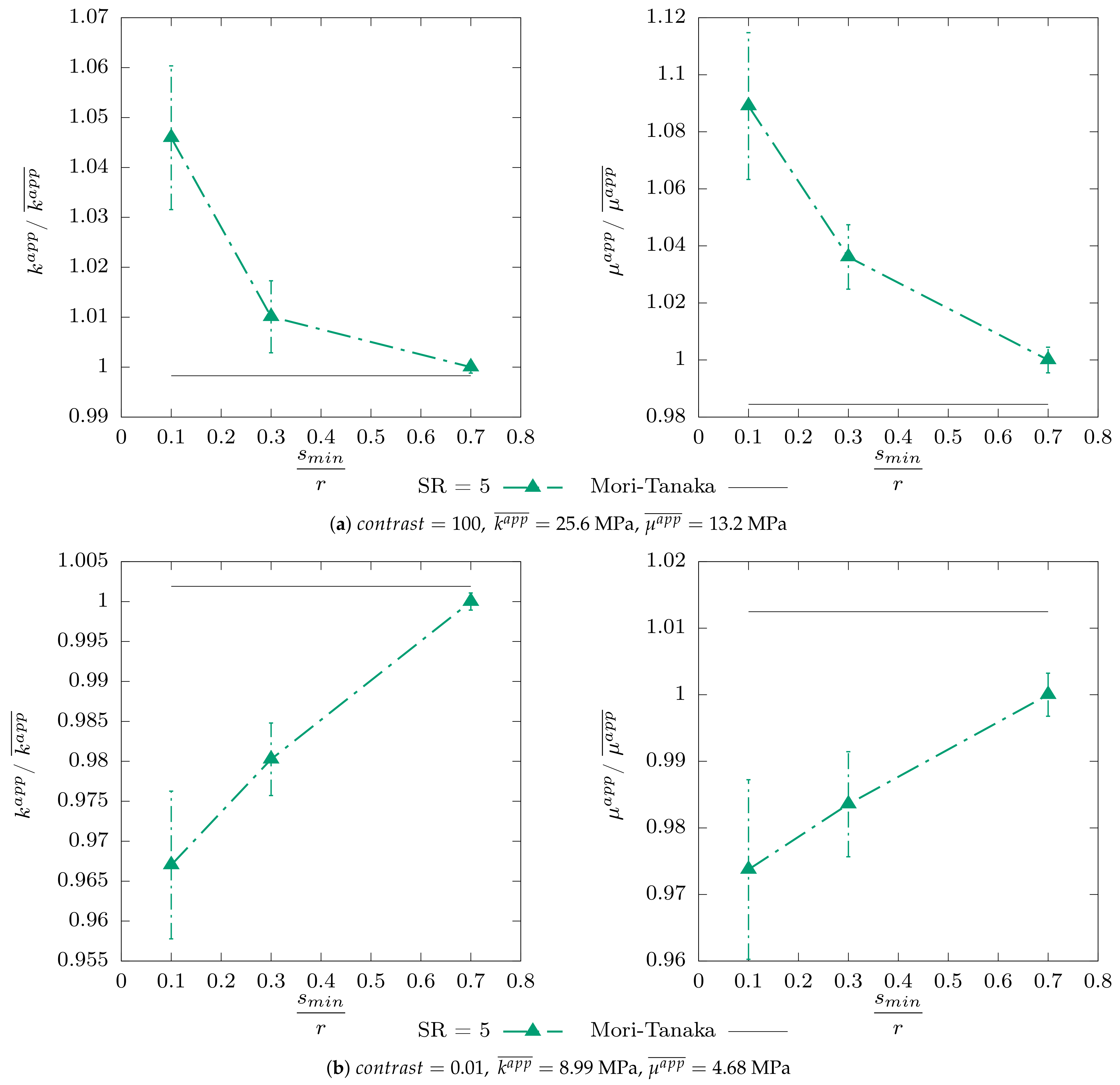
Appendix B. Complementary Results for the Effective Properties

Figure A1. Mean values and standard deviations on the mean value for the apparent moduli as a function of the packing parameter s m i n / r ( r = 10 μ m) for a volume fraction of inclusions f v = 13.4 %. For clarity, the error bars and dots are slightly shifted around for each studied minimum distance.
Mathematics 10 04437 g0a1
Figure A2. Mean values and standard deviations on the mean value for the apparent moduli as a function of the packing parameter s m i n / r ( r = 5 μ m) for a volume fraction of inclusions f v = 13.4 %. For clarity, the error bars and dots are slightly shifted around for each studied minimum distance.
Mathematics 10 04437 g0a2

Appendix C. Complementary Results for Mean Fields

Appendix C.1. First Moment

Figure A3. Mean values and standard deviations on the mean value for the first moment of hydrostatic stress by phase as a function of the packing parameter s m i n / r ( r = 10 μ m) for a volume fraction of inclusions f v = 13.4 %. For clarity, the error bars and dots are slightly shifted around for each studied minimum distance.
Mathematics 10 04437 g0a3
Figure A4. Mean values and standard deviations on the mean value for the first moment of hydrostatic stress by phase as a function of the packing parameter s m i n / r ( r = 10 μ m) for a volume fraction of inclusions f v = 25.1 %.
Mathematics 10 04437 g0a4
Figure A5. Mean values and standard deviations on the mean value for the first moment of equivalent stress by phase as a function of the packing parameter s m i n / r ( r = 10 μ m) for a volume fraction of inclusions f v = 13.4 %. For clarity, the error bars and dots are slightly shifted around for each studied minimum distance.
Mathematics 10 04437 g0a5

Appendix C.2. Second Moment

Figure A6. Mean values and standard deviations on the mean value for the second moment of hydrostatic stress by phase as a function of the packing parameter s m i n / r ( r = 10 μ m) for a volume fraction of inclusions f v = 13.4 %. For clarity, the error bars and dots are slightly shifted around for each studied minimum distance.
Mathematics 10 04437 g0a6
Figure A7. Mean values and standard deviations on the mean value for the second moment of hydrostatic stress by phase as a function of the packing parameter s m i n / r ( r = 10 μ m) for a volume fraction of inclusions f v = 25.1 %.
Mathematics 10 04437 g0a7
Figure A8. Mean values and standard deviations on the mean value for the second moment of equivalent stress by phase as a function of the packing parameter s m i n / r ( r = 10 μ m) for a volume fraction of inclusions f v = 13.4 %. For clarity, the error bars and dots are slightly shifted around for each studied minimum distance.
Mathematics 10 04437 g0a8

Appendix D. Complementary Results for Local Fields

Figure A9. Frequency histograms of equivalent stress by phase at S R = 10 , f v = 13.4 %, and the extreme s m i n values ( s m i n = 0.1 r and s m i n = 1.2 r ) for contrasts of 10 and 0.1.
Mathematics 10 04437 g0a9
Figure A10. Local equivalent stress at S R = 10 , f v = 13.4 % for extreme s m i n values and contrasts of 10 and 0.1—the cross-sectional views of an RVE.
Mathematics 10 04437 g0a10

References

  1. Gierden, C.; Kochmann, J.; Waimann, J.; Svendsen, B.; Reese, S. A Review of FE-FFT-Based Two-Scale Methods for Computational Modeling of Microstructure Evolution and Macroscopic Material Behavior. Arch. Comput. Methods Eng. 2022, 29, 4115–4135. [Google Scholar] [CrossRef]
  2. Hershey, A.V. The Elasticity of an Isotropic Aggregate of Anisotropic Cubic Crystals. J. Appl. Mech. 1954, 21, 236–240. [Google Scholar] [CrossRef]
  3. Mori, T.; Tanaka, K. Average stress in matrix and average elastic energy of materials with misfitting inclusions. Acta Metall. 1973, 21, 571–574. [Google Scholar] [CrossRef]
  4. Christensen, R.; Lo, K. Solutions for effective shear properties in three phase sphere and cylinder models. J. Mech. Phys. Solids 1979, 27, 315–330. [Google Scholar] [CrossRef]
  5. Masson, R.; Seck, M.; Fauque, J.; Garajeu, M. A modified secant formulation to predict the overall behavior of elasto-viscoplastic particulate composites. J. Mech. Phys. Solids 2020, 137, 103874. [Google Scholar] [CrossRef] [Green Version]
  6. Ponte Castañeda, P. Stationary variational estimates for the effective response and field fluctuations in nonlinear composites. J. Mech. Phys. Solids 2016, 96, 660–682. [Google Scholar] [CrossRef] [Green Version]
  7. Feyel, F. A multilevel finite element method (FE2) to describe the response of highly non-linear structures using generalized continua. Comput. Methods Appl. Mech. Eng. 2003, 192, 3233–3244. [Google Scholar] [CrossRef]
  8. Abdulle, A.; Weinan, E.; Engquist, B.; Vanden-Eijnden, E. The heterogeneous multiscale method. Acta Numer. 2012, 21, 1–87. [Google Scholar] [CrossRef] [Green Version]
  9. Michel, J.; Suquet, P. Nonuniform transformation field analysis. Int. J. Solids Struct. 2003, 40, 6937–6955. [Google Scholar] [CrossRef] [Green Version]
  10. Liu, L.; Bessa, M.; Liu, W. Self-consistent clustering analysis: An efficient multi-scale scheme for inelastic heterogeneous materials. Comput. Methods Appl. Mech. Eng. 2016, 306, 319–341. [Google Scholar] [CrossRef]
  11. Fritzen, F.; Leuschner, M. Reduced basis hybrid computational homogenization based on a mixed incremental formulation. Comput. Methods Appl. Mech. Eng. 2013, 260, 143–154. [Google Scholar] [CrossRef]
  12. Torquato, S. Morphology and effective properties of disordered heterogeneous media. Int. J. Solids Struct. 1998, 35, 2385–2406. [Google Scholar] [CrossRef]
  13. El Moumen, A.; Kanit, T.; Imad, A.; El Minor, H. Effect of overlapping inclusions on effective elastic properties of composites. Mech. Res. Commun. 2013, 53, 24–30. [Google Scholar] [CrossRef]
  14. Majewski, M.; Kursa, M.; Holobut, P.; Kowalczyk-Gajewska, K. Micromechanical and numerical analysis of packing and size effects in elastic particulate composites. Compos. Part B Eng. 2017, 124, 158–174. [Google Scholar] [CrossRef]
  15. Majewski, M.; Hołobut, P.; Kursa, M.; Kowalczyk-Gajewska, K. Packing and size effects in elastic-plastic particulate composites: Micromechanical modelling and numerical verification. Int. J. Eng. Sci. 2020, 151, 103271. [Google Scholar] [CrossRef]
  16. Bornert, M.; Stolz, C.; Zaoui, A. Morphologically representative pattern-based bounding in elasticity. J. Mech. Phys. Solids 1996, 44, 307–331. [Google Scholar] [CrossRef]
  17. Torquato, S. Single-Inclusion Solutions. In Random Heterogeneous Materials: Microstructure and Macroscopic Properties; Springer: New York, NY, USA, 2002; pp. 437–458. [Google Scholar] [CrossRef]
  18. Idiart, M.; Moulinec, H.; Ponte Castañeda, P.; Suquet, P. Macroscopic behavior and field fluctuations in viscoplastic composites: Second-order estimates versus full-field simulations. J. Mech. Phys. Solids 2006, 6, 201–208. [Google Scholar] [CrossRef] [Green Version]
  19. Kanit, T.; Forest, S.; Galliet, I.; Mounoury, V.; Jeulin, D. Determination of the size of the representative volume element for random composites: Statistical and numerical approach. Int. J. Solids Struct. 2003, 40, 3647–3679. [Google Scholar] [CrossRef]
  20. El Moumen, A.; Kanit, T.; Imad, A. Numerical evaluation of the representative volume element for random composites. Eur. J. Mech. A/Solids 2021, 86, 104181. [Google Scholar] [CrossRef]
  21. Plancq, D.; Thouvenin, G.; Ricaud, J.; Struzik, C.; Helfer, T.; Bentejac, F.; Thévenin, P.; Masson, R. PLEIADES: A unified environment for multi-dimensional fuel performance modeling. In Proceedings of the International Meeting on LWR Fuel Performance, Orlando, FL, USA, 19–22 September 2004. [Google Scholar]
  22. Marelle, V.; Michel, B.; Sercombe, J.; Goldbronn, P.; Struzik, C.; Boulore, A. Advanced Simulation of Fuel Behavior Under Irradiation in the PLEIADES Software Environment. In Modelling of Water Cooled Fuel Including Design Basis and Severe Accidents, Proceedings of the Technical Meeting, Chengdu, China, 28 October–1 November 2013; IAEA TECDOC SERIES, IAEA-TECDOC-CD–1775; IAEA: Vienna, Austria, 2013. [Google Scholar]
  23. Williams, S.; Philipse, A. Random Packings of Spheres and Spherocylinders Simulated by Mechanical Contraction. Phys. Rev. E Stat. Nonlinear Soft Matter Phys. 2003, 67, 051301. [Google Scholar] [CrossRef] [Green Version]
  24. Cooper, D. Random-sequential-packing simulations in three dimensions for spheres. Phys. Rev. A 1988, 38, 522–524. [Google Scholar] [CrossRef]
  25. Bourcier, C.; Dridi, W.; Chomat, L.; Laucoin, E.; Bary, B.; Adam, E. Combs: Open source python library for RVE generation. Application to microscale diffusion simulations in cementitious materials. In Proceedings of the Joint International Conference on Supercomputing in Nuclear Applications and Monte Carlo 2013 (SNA + MC 2013), Paris, France, 27–31 October 2013. [Google Scholar] [CrossRef]
  26. SALOME Platform. Available online: https://www.salome-platform.org/ (accessed on 1 July 2022).
  27. Schneider, M.; Josien, M.; Otto, F. Representative volume elements for matrix-inclusion composites—A computational study on the effects of an improper treatment of particles intersecting the boundary and the benefits of periodizing the ensemble. J. Mech. Phys. Solids 2022, 158, 104652. [Google Scholar] [CrossRef]
  28. Ramière, I.; Masson, R.; Michel, B.; Bernaud, S. Un schéma de calcul multi-échelles de type Éléments Finis au carré pour la simulation de combustibles nucléaires hétérogènes. In Proceedings of the 13e Colloque National en Calcul des Structures, Giens, France, 13–17 May 2013; Université Paris-Saclay, CSMA: Giens, Var, France, 2017. (In French). [Google Scholar]
  29. Ramière, I. Around Numerical Methods for Multiphysics and Multiscale Couplings in Solid Mechanics. Habilitation Thesis, Aix Marseille University (AMU), Marseille, France, 2021. [Google Scholar]
  30. Christensen, R.M. A critical evaluation for a class of micro-mechanics models. J. Mech. Phys. Solids 1990, 38, 379–404. [Google Scholar] [CrossRef]
  31. Hashin, Z.; Shtrikman, S. A variational approach to the theory of the elastic behaviour of multiphase materials. J. Mech. Phys. Solids 1963, 11, 127–140. [Google Scholar] [CrossRef]
  32. Cast3M. Available online: http://www-cast3m.cea.fr/ (accessed on 1 July 2022).
  33. Gloria, A.; Neukamm, S.; Otto, F. Quantification of ergodicity in stochastic homogenization: Optimal bounds via spectral gap on Glauber dynamics. Invent. Math. 2014, 199, 455–515. [Google Scholar] [CrossRef] [Green Version]
  34. Odegard, G.; Clancy, T.; Gates, T. Modeling of the mechanical properties of nanoparticle/polymer composites. Polymer 2005, 46, 553–562. [Google Scholar] [CrossRef]
  35. Zerhouni, O.; Brisard, S.; Danas, K. Quantifying the effect of two-point correlations on the effective elasticity of specific classes of random porous materials with and without connectivity. Int. J. Eng. Sci. 2021, 166, 103520. [Google Scholar] [CrossRef]
  36. Rasool, A.; Böhm, H.J. Effects of particle shape on the macroscopic and microscopic linear behaviors of particle reinforced composites. Int. J. Eng. Sci. 2012, 58, 21–34. [Google Scholar] [CrossRef]
Figure 1. Cross-sectional views of RVE mesh for extreme s m i n values, with close-ups of inclusions at s m i n , S R = 10 , r = 10 μ m, f v = 13.4 %.
Mathematics 10 04437 g001
Figure 2. Mean values and standard deviations on the mean value for the apparent moduli as a function of the packing parameter s m i n / r ( r = 10 μ m) for a volume fraction of inclusions f v = 13.4 %. For clarity, the error bars and dots are slightly shifted around for each studied minimum distance.
Mathematics 10 04437 g002
Figure 3. Mean distance between two spheres s m e a n as a function of s m i n for different scaling ratios. For clarity, the error bars and dots are slightly shifted around for each studied minimum distance.
Mathematics 10 04437 g003
Figure 4. Mean values and standard deviations on the mean value for the apparent moduli as a function of the packing parameter s m i n / r ( r = 10 μ m) for a volume fraction of inclusions f v = 25.1 %.
Mathematics 10 04437 g004
Figure 5. Mean values and standard deviations on the mean value for the first moment of hydrostatic stress by phase as a function of the packing parameter s m i n / r ( r = 10 μ m) for a volume fraction of inclusions f v = 13.4 %. For clarity, the error bars and dots are slightly shifted around for each studied minimum distance.
Mathematics 10 04437 g005
Figure 6. Mean values and standard deviations on the mean value for the first moment of equivalent stress by phase as a function of the packing parameter s m i n / r ( r = 10 μ m) for a volume fraction of inclusions f v = 13.4 %. For clarity, the error bars and dots are slightly shifted around for each studied minimum distance.
Mathematics 10 04437 g006
Figure 7. Mean values and standard deviations on the mean value for the second moment of hydrostatic stress by phase as a function of the packing parameter s m i n / r ( r = 10 μ m) for a volume fraction of inclusions f v = 13.4 %. For clarity, the error bars and dots are slightly shifted around for each studied minimum distance.
Mathematics 10 04437 g007
Figure 8. Mean values and standard deviations on the mean value for the second moment of equivalent stress by phase as a function of the packing parameter s m i n / r ( r = 10 μ m) for a volume fraction of inclusions f v = 13.4 %. For clarity, the error bars and dots are slightly shifted around for each studied minimum distance.
Mathematics 10 04437 g008
Figure 9. Frequency histograms of equivalent stress by phase at S R = 10 , f v = 13.4 %, and the extreme s m i n values ( s m i n = 0.1 r and s m i n = 1.2 r ) for contrasts of 0.01 and 100.
Mathematics 10 04437 g009
Figure 10. Local equivalent stress at S R = 10 , f v = 13.4 % for extreme s m i n values and contrasts of 100 and 0.01—the cross-sectional views of RVE.
Mathematics 10 04437 g010
Table 1. Mesh convergence of k a p p , S R = 2.5 , f v = 13.4 %, c o n t r a s t = 100 .
n min = 2 g = 2
g = 1 . 15 g = 1 . 5 g = 2 n min = 3 n min = 4
k a p p (MPa)20.91620.91820.92020.91420.919
Standard deviation of k a p p (MPa)0.4610.4620.4630.4680.460
Number of nodes279,00065,30032,50088,900158,700
Table 2. Average number of nodes in the mesh and number of samples with inclusion volume fraction f v = 13.4 % for different scaling ratios S R with r = 10 μ m.
SR = 2.5 SR = 5 SR = 10
Number of nodes30,000300,0002,500,000
Number of samples3507035
Publisher’s Note: MDPI stays neutral with regard to jurisdictional claims in published maps and institutional affiliations.

