Polynomial Fuzzy Information Granule-Based Time Series Prediction

Abstract

Fuzzy information granulation transfers the time series analysis from the numerical platform to the granular platform, which enables us to study the time series at a different granularity. In previous studies, each fuzzy information granule in a granular time series can reflect the average, range, and linear trend characteristics of the data in the corresponding time window. In order to get a more general information granule, this paper proposes polynomial fuzzy information granules, each of which can reflect both the linear trend and the nonlinear trend of the data in a time window. The distance metric of the proposed information granules is given theoretically. After studying the distance measure of the polynomial fuzzy information granule and its geometric interpretation, we design a time series prediction method based on the polynomial fuzzy information granules and fuzzy inference system. The experimental results show that the proposed prediction method can achieve a good long-term prediction.

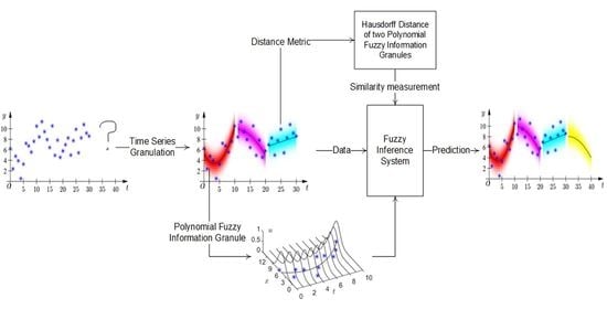
1. Introduction

Time series prediction has been a classic machine learning task widely studied in recent years, and it has been applied to many fields, such as business [1], engineering [2], energy [3], and so on. It is hoped that some prediction methods can be used to find the internal association rules of the time series to predict the future changes.

Popular time series prediction methods include classical time series models, such as linear regression, autoregression, and moving average [4,5], as well as artificial intelligence methods, such as support vector regression (SVR) [6], artificial neural networks (ANNs) [7], nonlinear autoregressive (NAR) [8], recurrent neural networks (RNNs) [9,10], long short-term memory (LSTM) networks [11,12], and so on. The classical time series models usually require the data to be analyzed to meet the ergodicity, stationarity, and other assumptions [13], and these strict conditions may not always hold for real world data. Although many intelligent methods such as SVR and ANNs come with the ability to capture the nonlinear relationship between the input and output variables, and have been applied to solve many real-word problems [14,15,16,17], the quality of their prediction depends very much on the data set to be processed [18]. These numerical prediction methods are computationally expensive and more suitable for a short-term prediction. In addition, the lack of interpretability of these numerical methods has become the main barrier in their wide acceptance in time series prediction applications. These methods, as well as their results, are not easy to be understood by humans.

The fuzzy information granulation of the time series [19,20] is one of the feasible methods to solve the above shortcomings. In this method, a time series is firstly divided into some meaningful time windows in the time dimension, and then a fuzzy information granule (FIG) is established on each time window. In this way, a time series is transformed to a sequence of FIGs, each of which is a fuzzy set, and the time series can be now analyzed at the granular level by directly manipulating the FIGs. The combination of an FIG with fuzzy reasoning [21], a support vector machine [22], and other artificial intelligence algorithms for data mining [23,24,25] has become one of the research hotspots in recent years.

An FIG is usually represented by a fuzzy set, whose membership function is defined on the real number axis. Common forms of the membership functions of FIGs include the interval membership function, triangular membership function, and Gaussian membership function [26,27,28], and the corresponding FIGs are called Interval FIG(IFIG), Triangular FIG(TFIG), and Gaussian FIG(GFIG) in this paper, respectively. These types of FIGs can reflect the characteristics of the average and range of the temporal data in a time window, but fail to reflect the trend characteristic of the data.

As a modification, the linear fuzzy information granule (LFIG) [29] is represented by a fuzzy set whose membership function is defined both on the real number axis and the time axis. Like the LFIG, the polar fuzzy information granule (polar FIG) [30] defines its membership function in two-dimensional polar coordinates. Compared with the FIG, the added dimension in the membership functions of the LFIG and the polar FIG makes them possible to express the linear changing trends of the samples in the time window. However, both modifications failed to reflect the nonlinear trends of the samples.

In [31], a novel Gaussian-type time-variant FIG, named the generalized zonary time-variant FIG (GZTFIG), was proposed which can reflect the nonlinear trend of data changing. However, the form of the GZTFIG is a bit complex. In addition, GZTFIGs have a lack of specificity [32], that is, their semantics are not so clear.

To solve this problem, based on [29,31], this paper introduces a novel FIG, namely, the polynomial fuzzy information granule (PFIG), which represents the temporal samples in a time window by three kinds of parameters: (1) the length of the time window, (2) a polynomial center line, and (3) the degree of data deviation from the center line. Temporal samples can be reasonably characterized by the polynomial center line with an adjustable order. In the sense of the Hausdorff distance, the distance formula of the PFIG is derived theoretically. In particular, we prove that the distance of the two Gaussian PFIGs has a concise formula expression and intuitive geometric interpretation. Therefore, the PFIG is a well-defined information granule with a good distance property, which is hopeful to become an effective tool in time series granulation and prediction.

The remainder of this paper is organized as follows. Section 2 introduces traditional fuzzy information granules and their distance measure. Section 3 introduces PFIGs as well as their distance measure. It can be proved that the distance of Gaussian PFIGs have a simple formula, which corresponds to a reasonable geometric interpretation. Section 4 presents a long-term prediction method for the time series based on the distance measure of PFIGs and fuzzy inference system with an interpolation scheme. Section 5 describes three experiments to verify the effectiveness and feasibility of the proposed model. Finally, Section 6 provides the conclusions and offers some thoughts on future studies.

2. Fuzzy Information Granules and Their Distance

In this section, we briefly introduce the construction method of some common FIGs along with their distance measurement. These concepts are useful for defining the novel type of granule (PFIG) given in Section 3.

2.1. Fuzzy Numbers and Their Distance Measurement

A fuzzy set (class) $A$ in $X$ is characterized by a membership (characteristic) function $f_A\left(x\right)$ which associates with each point in $X$ a real number in the interval [0,1] [33]. Fuzzy numbers are special fuzzy sets. A fuzzy set $A$ is called a fuzzy number if its membership function $A\left(x\right)$ satisfies the following conditions [34]:

(a)

$A$ is normal: there exists a number $x_0\in R,$ such that $A\left(x_0\right)=1$;

(b)

$A$ is convex: $A\left(\omega x_1+\left(1-\omega \right)x_2\right)\ge \min \left\{A\left(x_1\right),A\left(y_2\right)\right\},\forall \omega \in \left[0,1\right],\forall x_1$,$x_2\in R$;

(c)

$A$ is upper semicontinuous: $\forall \epsilon >0$, $\exists \delta >0$, if $x\in \dot{U}\left(x_0,\delta \right)$, then $A\left(x\right)-A\left(x_0\right)<\epsilon$.

(d)

$A$ is compactly supported: the closure of the set $\left\{x|A\left(x\right)\rangle 0\right\}$ is compact.

Figure 1 shows examples of one-dimensional and two-dimensional fuzzy numbers.

Fuzzy numbers generalize classical real intervals. Accordingly, the distance of the fuzzy numbers can also be extended from the Hausdorff distance of the real number intervals. Named after Felix Hausdorff, the Hausdorff distance is a generalized metric in the family of closed sets, which measures the maximum distance of a set to the nearest point in the other set [35]. Let $A\left(\lambda \right)=\left\{x\in R|u\left(x\right)\ge \lambda \right\}$ be the $\lambda$-level set (or called $\lambda$-cut) of fuzzy number $A$. Since the $\lambda$-level sets $A\left(\lambda \right)$ and $B\left(\lambda \right)$ of fuzzy numbers $A$ and $B$ are classical real intervals, their Hausdorff distance can be written as:

$$d\left(A\left(\lambda \right),B\left(\lambda \right)\right)=\max \left\{\underset{x\in A\left(\lambda \right)}{\sup }\underset{y\in B\left(\lambda \right)}{\inf }d\left(x,y\right), \underset{y\in B\left(\lambda \right)}{\sup }\underset{x\in A\left(\lambda \right)}{\inf }d\left(x,y\right)\right\},$$

(1)

where $d\left(x,y\right)$ represents the distance of real numbers $x$ and $y$. Based on such a distance for real sets, the Hausdorff distance of fuzzy numbers $A$ and $B$ can be defined as [36]:

$$d\left(A,B\right)={\int }_0^{1}d\left(A\left(\lambda \right),B\left(\lambda \right)\right)\mathrm{d}\lambda .$$

(2)

2.2. Fuzzy Information Granules and Their Distance

Constructing an FIG $A$ to represent a group of temporal data $\mathit{y}=\left\{y_1,y_2,\cdots ,y_n\right\}$ should comply with the following two fairly conflicting conditions [32]. The first condition is called representativeness, that is, $A$ should embrace enough data in $\mathit{y}$. In another word, the total membership of $\mathit{y}$ belonging to $A$, $\sum _{i=1}^{n}A\left(y_i\right)$, should be as large as possible, so that $A$ has a good data coverage. The second condition is called specificity, that is, $A$ should be specific enough. This is accomplished by keeping the support of $A$ as compact (small) as possible, so that $A$ has a better semantic clarity [32]. According to the types of membership functions, FIGs can be divided into Interval FIGs (IFIGs), Triangular FIGs (TFIGs), Gaussian FIGs (GFIGs), etc. Denote the membership function of an FIG $A$ as $A\left(x;\mathit{\gamma }\right)$, where $\mathit{\gamma }$ is the parameter set of the membership function of the corresponding type. The optimal value of $\mathit{\gamma }$ can be determined by optimizing both the representativeness and the specificity of the FIG $A\left(\mathit{\gamma }\right)$ through the optimization methods described below [32].

2.2.1. Interval Fuzzy Information Granules and Their Distance

An IFIG, denoted as $A_I\left(a,b\right)$ or $I\left(a,b\right)$, comes with the following membership function:

$$A_I\left(x;a,b\right)=I\left(x;a,b\right)=\{\begin{array}{cc}1,& x\in \left[a,b\right],\\ 0,& \mathrm{else}.\end{array}$$

(3)

Let $\mathit{\gamma }=\left\{a,b\right\}$ be the parameter set of this membership function, $a \mathrm{and} b$ are the left and right boundary points of the interval-type membership function, which can be determined by the following optimization model:

$$\underset{a,b}{\max }\frac{{\sum }_{y_i}\left(2\cdot I\left(y_i;a,b\right)-1\right)}{\left|b-a\right|}.$$

(4)

The numerator part of Equation (4) is related to the number of data $\mathit{y}$ that belong to the IFIG $I\left(a,b\right)$. Maximizing the numerator part can make $I\left(a,b\right)$ achieve the best data coverage or representativeness. The denominator part of Equation (4) is related to the support of $A$. Minimizing the denominator part can make $I\left(a,b\right)$ achieve the best specificity.

As far as the distance of two IFIGs is concerned, according to Equations (1) and (2), the distance of $I_1\left(a_1,b_1\right)$ and $I_2\left(a_2,b_2\right)$ can be written as:

$$d\left(I_1,I_2\right)=\max \left\{\left|a_1-a_2\right|,\left|b_1-b_2\right|\right\}.$$

(5)

2.2.2. Triangular Fuzzy Information Granules and Their Distance

A TFIG, denoted as $A_T\left(a,m,b\right)$ or $T\left(a,m,b\right)$, comes with the following membership function:

$$A_T\left(x;a,m,b\right)=T\left(x;a,m,b\right)=\{\begin{array}{cc}\frac{x-a}{m-a},& a<x<m,\\ \frac{x-b}{m-b},& m\le x<b,\\ 0,& \mathrm{else}.\end{array}$$

(6)

Let $\mathit{\gamma }=\left\{a,m,b\right\}$ be the parameter set of $T\left(a,m,b\right)$, where $a, m,$ and $b$ are called the “left extreme point”, the “normal point”, and the “right extreme point”, respectively. $m$ can be determined as the median of $\mathit{y}$, and the extreme points $a$ and $b$ can be determined by the following optimization model [37]:

$$\underset{a,b}{\max } \frac{{\sum }_{y_i\le m}\frac{y_i-a}{m-a}}{m-a}+\frac{{\sum }_{y_i>m}\frac{b-y_i}{b-m}}{b-m}.$$

(7)

The numerator part of Equation (7) is related to the total membership degrees of $\mathit{y}$ belonging to $A$, which reflects the representativeness of $T\left(a,m,b\right)$ to $\mathit{y}$. Maximizing the numerator part can make $T\left(a,m,b\right)$ achieve the best representativeness. The denominator part of Equation (7) is related to the support of $A$. Minimizing the denominator part can make $T\left(a,m,b\right)$ achieve the best specificity.

As far as the distance of two TFIGs is concerned, according to Equations (1) and (2), the distance of $T_1\left(a_1,m_1,b_1\right)$ and $T_2\left(a_2,m_2,b_2\right)$ can be written as:

$$d\left(T_1,T_2\right)=\frac{1}{2}\max \left\{\left|\left(a_1-a_2\right)+\left(m_1-m_2\right)\right|,\left|\left(b_1-b_2\right)+\left(m_1-m_2\right)\right|\right\}.$$

(8)

2.2.3. Gaussian Fuzzy Information Granules and Their Distance

A GFIG, denoted as $A_G\left(\mu ,\sigma \right)$ or $G\left(\mu ,\sigma \right)$, comes with the following membership function:

$$A_G\left(x;\mu ,\sigma \right)=G\left(x;\mu ,\sigma \right)=\exp \left(-\frac{{\left(x-\mu \right)}^2}{2{\sigma }^2}\right).$$

(9)

Let $\mathit{\gamma }=\left\{\mu ,\sigma \right\}$ be the parameter set of $G\left(\mu ,\sigma \right)$, where $\mu$ and $\sigma$ can be estimated by the mean value and standard deviation of $\mathit{y}$, respectively. The GFIG has a clear meaning, and compared with the TFIG, the GFIG has less parameters with simpler parameter determination methods. According to the extension principle [38], the linear operation of GFIGs has a concise calculation property. That is:

Theorem 1

([29]). For any two GFIGs $G_1\left({\mu }_1,{\sigma }_1\right), G_2\left({\mu }_2,{\sigma }_2\right)$ and any two real numbers ${\omega }_1,{\omega }_2\in R$, we have

$${\omega }_1{G}_1\left({\mu }_1,{\sigma }_1\right)+{\omega }_2{G}_2\left({\mu }_2,{\sigma }_2\right)=G\left({\omega }_1{\mu }_1+{\omega }_2{\mu }_2,{\omega }_1{\sigma }_1+{\omega }_2{\sigma }_2\right).$$

(10)

Furthermore, the Hausdorff distance of two GFIGs $G_1\left({\mu }_1,{\sigma }_1\right)$ and $G_2\left({\mu }_2,{\sigma }_2\right)$ can be concisely written as [29]:

$$d\left(G_1,G_2\right)=\mathsf{\Delta }u+\frac{\sqrt{2\pi } \mathsf{\Delta }\sigma }{2},$$

(11)

where $\mathsf{\Delta }\mu =\left|{\mu }_1-{\mu }_2\right|$ and $\mathsf{\Delta }\sigma =\left|{\sigma }_1-{\sigma }_2\right|$.

3. Polynomial Fuzzy Information Granules and Their Distance Metric

3.1. Polynomial Fuzzy Information Granules

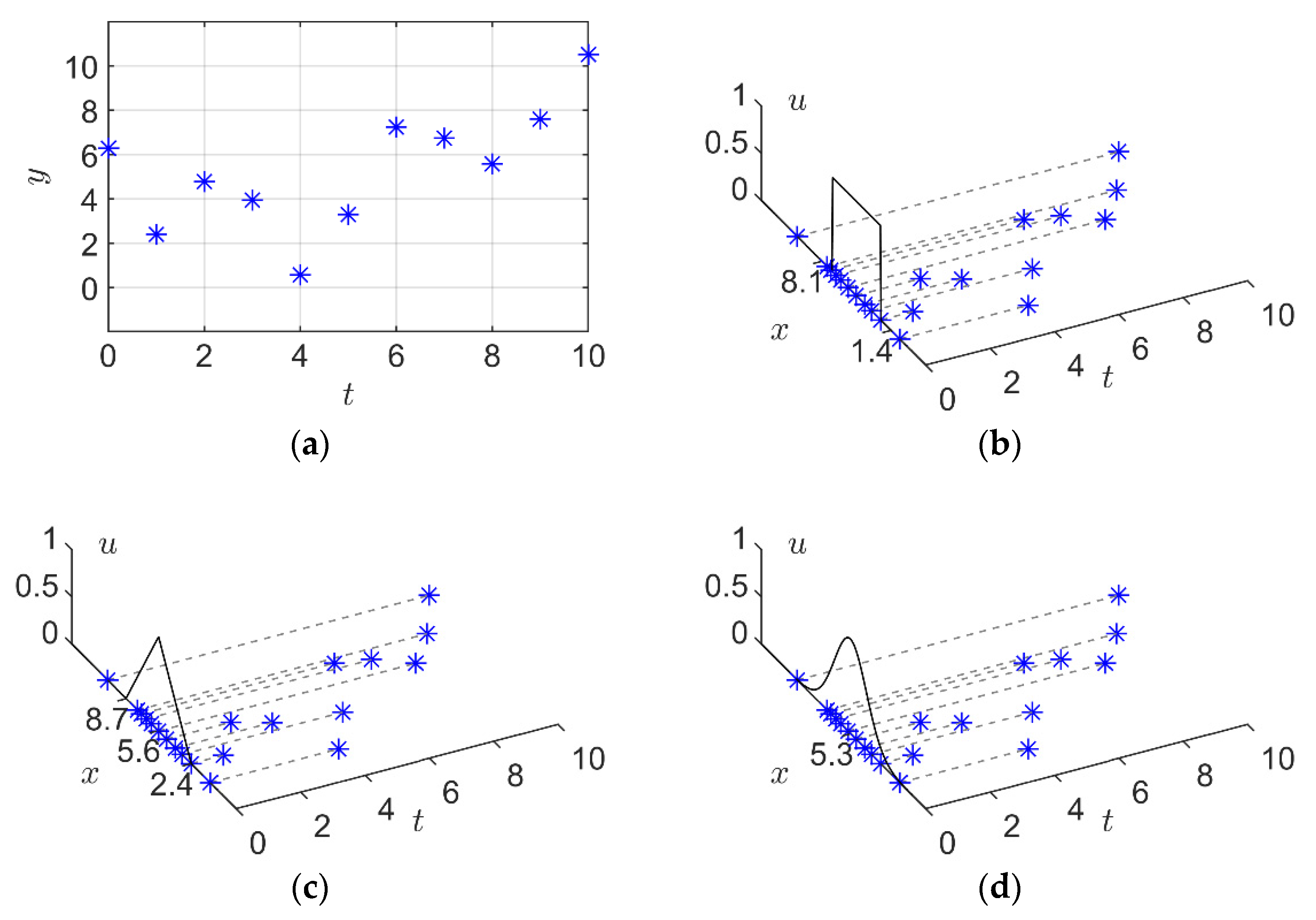
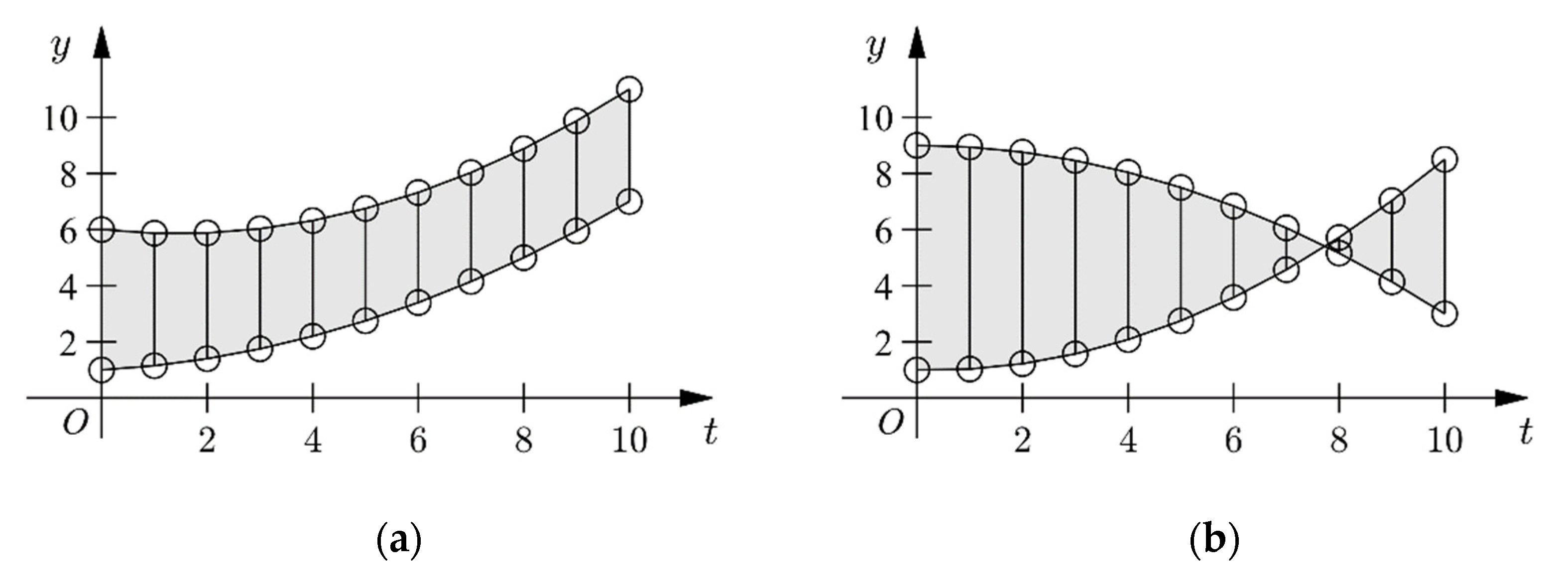
Suppose we are going to granulize a time series $\mathit{y}=\left\{\left(t,y_t\right),t=1,2,\cdots ,\tau \right\}$ as shown in Figure 2a. The IFIG, TFIG, and GFIG obtained by the corresponding granulation methods given by Equations (4), (7), and (9) in Section 2 are shown in Figure 2b–d, respectively. Because the membership functions of the IFIG, TFIG, and GFIG (as shown in Equations (3), (6), and (9)) are time-independent, their membership values of $\left(t,y_t\right)$ depend only on $y_t$. As a result, these FIGs can properly reflect the average and range information of $\mathit{y}$. However, they fail to reflect the changing trends of the time series, since the time-varying relationship between $y_t$ and $t$ is ignored.

One way to remedy this defect is to add the time variable $t$ to the membership functions of the FIGs. The two-dimensional membership function of an FIG can be obtained by shifting the one-dimensional membership function in Figure 2 along the time axis. Follow this mechanism, the LFIGs [29] accomplish this goal by making the membership function of the GFIG (as shown in Figure 2d) change linearly over time. The two-dimensional membership function of the LFIG is shown in Figure 3.

Motivated by the time variant LFIG, we define a novel class of FIG called polynomial fuzzy information granules (PFIG) in this paper. In order to fully reflect the time-varying characteristics of the data in the time window, a reasonable PFIG should contain three types of parameters:

• The length of the time series $\mathit{y}$, i.e., the size of time window, $\tau$;
• A time-variant $p$-order center (regression) curve line $y_t=f\left(t,\mathit{\beta }\right)={\beta }_0+{\beta }_{1}t+\cdots +{\beta }_p{t}^p$ that reflects the changing of the time series;
• The parameters reflecting the deviation degree of the temporal data from the center line.

Definition 1.

(PFIG) For a time series $\mathit{y}=\left\{\left(t,y_t\right),t=1,2,\cdots ,\tau \right\}$, a fuzzy information granule $P\left(\mathit{\beta },\tau ,\mathit{\gamma }\right)$ representing $\mathit{y}$ is called a PFIG of order $p$, if its membership function $P\left(\left(t,x\right);\mathit{\beta },\tau ,\mathit{\gamma }\right)$ has a center curve line:

$$f\left(t,\mathit{\beta }\right)={\beta }_0+{\beta }_{1}t+\cdots +{\beta }_p{t}^p, t\in \left[0,\tau \right],$$

(12)

and $P\left(\left(t,x\right);\mathit{\beta },\tau ,\mathit{\gamma }\right)$ can be written as:

$$P\left(\left(t,x\right);\mathit{\beta },\tau ,\mathit{\gamma }\right)=A\left(f\left(t,\mathit{\beta }\right);\mathit{\gamma }\right), t\in \left[0,\tau \right],$$

(13)

where $A$ is a fuzzy number, $A\left(x,\mathit{\gamma }\right)$ is its membership function, $\mathit{\gamma }$ is a parameter set of the PFIG that reflects the deviation degree of the data from the center line, and the length of the time series $\tau$ is called the granularity of the PFIG.

Recently, Luo proposed a novel generalized zonary time-variant FIG (GZTFIG) in [31], which is able to reflect the nonlinear trends of the time series. The membership function of a GZTFIG is defined as:

$$\begin{gathered} f\left(x;{\beta }_n,{\beta }_{n-1},\cdots {\beta }_1,{\beta }_0,\sigma ,{\underset{\_}{\beta }}_0,{\overline{\beta }}_0,\tau \right)=f\left(x;{\beta }_n{t}^n+{\beta }_{n-1}{t}^{n-1}+···+{\beta }_{1}t+{\beta }_0,\sigma \right) \\ =\exp \left(-\frac{{\left(x-\left({\beta }_n{t}^n+{\beta }_{n-1}{t}^{n-1}+···+{\beta }_{1}t+{\beta }_0\right)\right)}^2}{2{\sigma }^2}\right),{\beta }_0\in \left[{\underset{\_}{\beta }}_0,{\overline{\beta }}_0\right], \end{gathered}$$

where $\left[{\underset{\_}{\beta }}_0,{\overline{\beta }}_0\right]$ reflects the data fluctuation interval in the current time window. $\left[{\underset{\_}{\beta }}_0,{\overline{\beta }}_0\right]$ can be determined by making all the data in $\mathit{y}$ locate in the zonary area between the upper boundary ${\beta }_n{t}^n+{\beta }_{n-1}{t}^{n-1}+···+{\beta }_{1}t+{\overline{\beta }}_0$, and the lower boundary ${\beta }_n{t}^n+{\beta }_{n-1}{t}^{n-1}+···+{\beta }_{1}t+{\underset{\_}{\beta }}_0$.

Different from the GZTFIGs proposed in [31], the proposed PFIG no longer restricts its membership function to be Gaussian. Users can choose any appropriate type of membership function to construct a PFIG according to the characteristics of the time series. For the following three reasons, the PFIG uses the center curve line, instead of the zonal central region in the GZTFIG to reflect the changing trends of a time series. First, the width of the zonal region ${\overline{\beta }}_0-{\underset{\_}{\beta }}_0$ is to reflect the degree of data deviation from the center line. However, this feature can also be reflected by the parameter $\mathit{\gamma }$ in the PFIG, which is more concise. Secondarily, compared with GZTFIGs, the process of determining the zonary area is to avoid being in the PFIG. Thus, the construction of the PFIG is simpler. Last but not the least, the central zonary area of a GZTFIG is determined by translating the central line upward and downward, so that all the data are included in the zonary area. This operation increases the representativeness of the GZTFIG but decreases its specificity.

Using the definition of PFIGs, we can give the definitions for three special kinds of PFIGs, namely interval-type PFIGs (IPFIGs), triangular-type PFIGs (TPFIGs), and Gaussian-type PFIGs (GPFIGs).

Definition 2.

(IPFIG). A PFIG $P\left(\mathit{\beta },\tau ,\mathit{\gamma }\right)=I_p\left(\mathit{\beta },\tau ,r\right)$ is called an IPFIG of order $p$, if its membership function $P\left(\left(t,x\right);\mathit{\beta },\tau ,\mathit{\gamma }\right)$ can be written as:

$$I_p\left(\left(t,x\right);a\left(\mathit{\beta },t,r\right),b\left(\mathit{\beta },t,r\right)\right)=\{\begin{array}{cc}1,& x\in \left[a\left(\mathit{\beta },t,r\right),b\left(\mathit{\beta },t,r\right)\right],\\ 0,& \mathrm{else},\end{array}$$

where $a\left(\mathit{\beta },t,r\right)=f\left(t,\mathit{\beta }\right)-r$ and $b\left(\mathit{\beta },t,r\right)=f\left(t,\mathit{\beta }\right)+r$ are the left and right boundary points of the interval-type membership function at $t\in \left[0,\tau \right]$, respectively; $f\left(t,\mathit{\beta }\right)={\beta }_0+{\beta }_{1}t+\cdots +{\beta }_p{t}^p$ represents the center curve line of PFIG; and $r$ is the radius of this interval.

Definition 3.

(TPFIG): A PFIG $P\left(\mathit{\beta },\tau ,\mathit{\gamma }\right)=T_p\left(\mathit{\beta },\tau ,r_1,r_2\right)$ is called a TPFIG of order $p$ if its membership function $P\left(\left(t,x\right);\mathit{\beta },\tau ,\mathit{\gamma }\right)$ can be written as:

$$T_p\left(\left(t,x\right);a\left(\mathit{\beta },t,r_1\right),m\left(\mathit{\beta },t\right),b\left(\mathit{\beta },t,r_2\right)\right)=\{\begin{array}{cc}\frac{x-a}{m-a},& a\left(\mathit{\beta },t,r_1\right)<x<m\left(\mathit{\beta },t\right),\\ \frac{x-b}{m-b},& m\left(\mathit{\beta },t\right)\le x<b\left(\mathit{\beta },t,r_2\right),\\ 0,& \mathrm{else},\end{array}$$

where $m\left(\mathit{\beta },t\right)=f\left(t,\mathit{\beta }\right)={\beta }_0+{\beta }_{1}t+\cdots +{\beta }_p{t}^p$ represents the center curve line of the PFIG, and $a\left(\mathit{\beta },t,r_1\right)=m\left(\mathit{\beta },t\right)-r_1$ and $b\left(\mathit{\beta },t,r_2\right)=m\left(\mathit{\beta },t\right)+r_2$ are the left and right extreme points of the triangular membership function at $t\in \left[0,\tau \right]$, respectively.

Definition 4.

(GPFIG): A PFIG $P\left(\mathit{\beta },\tau ,\mathit{\gamma }\right)=G_p\left(\mathit{\beta },\tau ,\sigma \right)$ is called a GPFIG of order $p$ if its membership function $P\left(\left(t,x\right);\mathit{\beta },\tau ,\mathit{\gamma }\right)$ can be written as:

$$G_p\left(\left(t,x\right);\mathit{\beta },\tau ,\sigma \right)=\exp \left(-\frac{{\left(x-\mu \left(t,\mathit{\beta }\right)\right)}^2}{2{\sigma }^2}\right),$$

(14)

where $\mu \left(t,\mathit{\beta }\right)=f\left(t,\mathit{\beta }\right)$ is the center line of PFIG, and $\sigma$ is the standard deviation that reflects the degree of data deviation from the center line.

The construction of a GPFIG is straightforward. The center line $\mu \left(t;\mathit{\beta }\right)$ can be estimated by the polynomial regression of the temporal data $\mathit{y}=\left\{\left(t,y_t\right),t=1,2,\cdots ,\tau \right\}$, and $\sigma$ can be estimated by:

$${\sigma }^2=\frac{1}{\tau }{\displaystyle \sum }_{t=1}^{\tau }{\left(y_t-\mu \left(t;\mathit{\beta }\right)\right)}^2.$$

(15)

According to the above definitions, the temporal data in Figure 2a can be represented by a second order GPFIG as shown in Figure 4. Compared with the IFIG, TFIG, and GFIG shown in Figure 2b–d, the GPFIG can better reflect the changing trends in the temporal data, as shown in Figure 2a.

When the order of a PFIG is 0, the PFIG degenerates into the same type of FIGs introduced in Section 1, and when the order of a GPFIG is 1, the center line of the GPFIG becomes a linear function $f\left(t,\mathit{\beta }\right)={\beta }_0+{\beta }_{1}t$. Accordingly, the GPFIG degenerates into the LFIG proposed by [29]. Therefore, PFIGs, including GPFIGs, are a generalization of LFIGs.

A GPFIG is an information granule with good properties. From its definition, it can be found that the number of parameters of a GPFIG is small, its meaning is clear, and the Gaussian-type FIG has excellent operation properties, as shown in Theorem 1. In addition, the GPFIG is also easy to understand, given a GPFIG $G_p\left(\left(t,x\right);\mathit{\beta },\tau ,\sigma \right)$, we can imagine a time series of length $\tau$, distributed around a center curve line $f\left(t,\mathit{\beta }\right),t\in \left[0,\tau \right]$, with $\sigma$ as the deviation degree of the temporal data from the center line. Therefore, the GPFIG is a good tool to construct the information granule to describe a group of temporal data. For this reason, our experiments in Section 5 will focus only on the GPFIG.

3.2. Distance Metric of Polynomial Fuzzy Information Granules

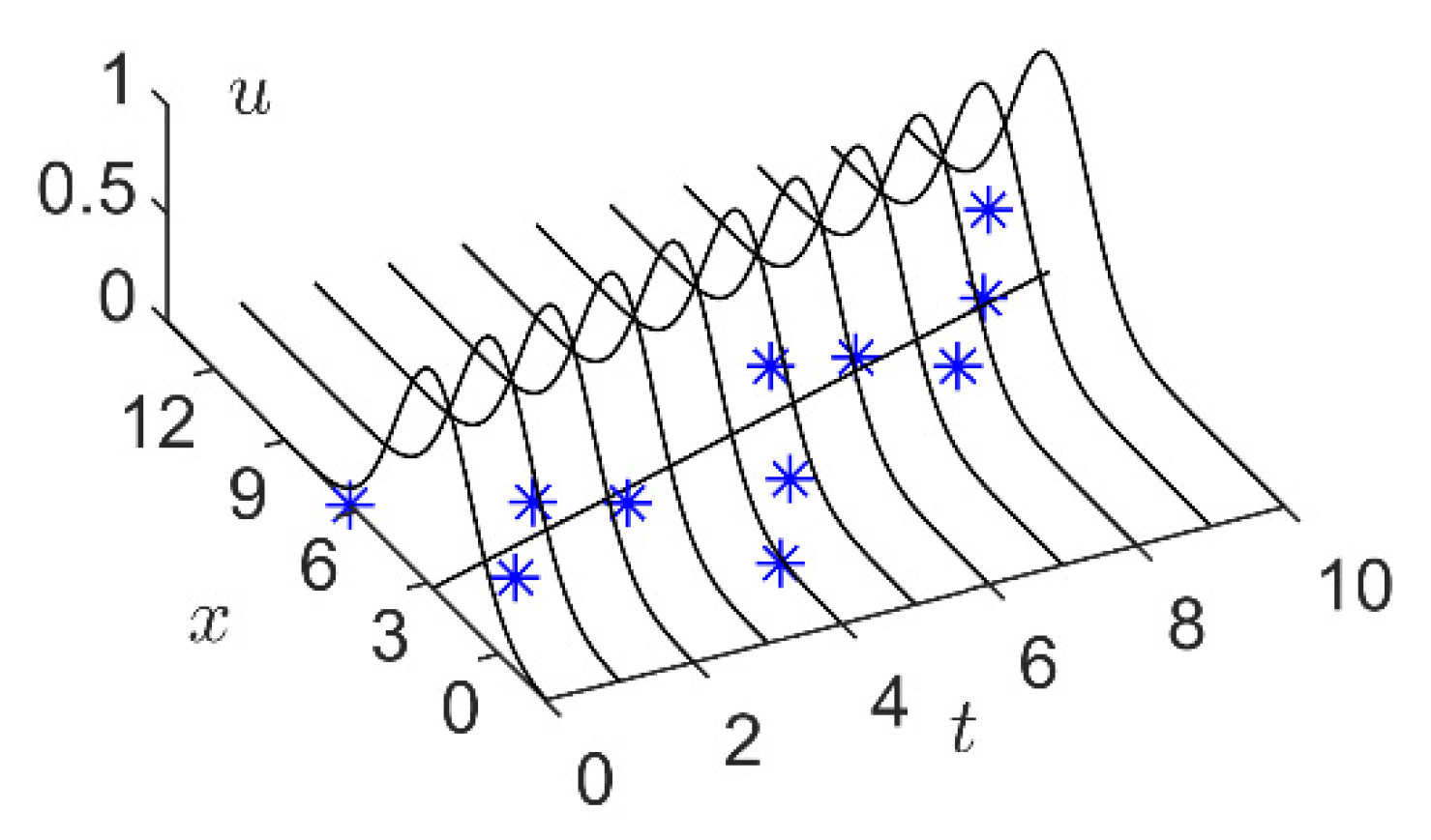
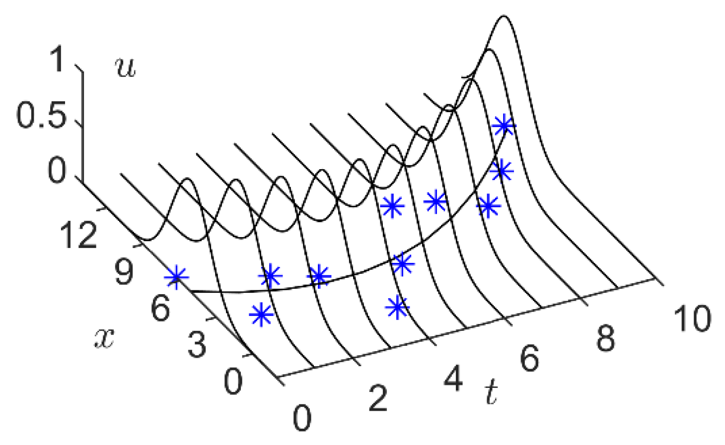
By comparing Figure 4 and Figure 1b, we can find that the PFIG is a special type of two-dimensional fuzzy set. For a PFIG $P\left(\mathit{\beta },\tau ,\mathit{\gamma }\right)$, its membership function is a two-dimensional convex surface. As shown in Figure 5, the $\lambda$-level set of $P\left(\mathit{\beta },\tau ,\mathit{\gamma }\right)$ is:

$$P\left(\lambda \right)=\left\{\left(t,x\right)|P\left(\left(t,x\right);\mathit{\beta },\tau ,\mathit{\gamma }\right)\ge \lambda \right\},$$

(16)

which can be regarded as a two-dimensional closed interval in the time-number plane ($t$-$x$ plane).

Similar to Equation (2), define the distance of two PFIGs $P_1\left({\mathit{\beta }}_1,\tau ,{\mathit{\gamma }}_1\right)$ and $P_2\left({\mathit{\beta }}_2,\tau ,{\mathit{\gamma }}_2\right)$ as the sum of all the distances of the $\lambda$-level sets [36]:

$$d\left(P_1,P_2\right)={\int }_0^{1}d\left(P_1\left(\lambda \right),P_2\left(\lambda \right)\right)\mathrm{d}\lambda ,$$

(17)

where $d\left(P_1\left(\lambda \right),P_2\left(\lambda \right)\right)$ is the Hausdorff distance of two-dimensional closed intervals $P_1\left(\lambda \right)$ and $P_2\left(\lambda \right)$, which can be written as:

$$d\left(P_1\left(\lambda \right),P_2\left(\lambda \right)\right)=\max \left\{\underset{z_1\in P_1\left(\lambda \right)}{\sup }\underset{z_2\in P_2\left(\lambda \right)}{\inf }d\left({\mathit{z}}_1,{\mathit{z}}_2\right), \underset{z_2\in P_2\left(\lambda \right)}{\sup }\underset{z_1\in P_1\left(\lambda \right)}{\inf }d\left({\mathit{z}}_1,{\mathit{z}}_2\right)\right\},$$

(18)

where ${\mathit{z}}_1=\left(t_1,x_1\right)\in P_1\left(\lambda \right)\mathrm{and}{\mathit{z}}_2=\left(t_2,x_2\right)\in P_2\left(\lambda \right)$.

The calculation of Equation (18) is very complex and is computationally difficult to implement. To solve this problem, we should redefine $d\left(P_1\left(\lambda \right),P_2\left(\lambda \right)\right)$ based on the following considerations. The Hausdorff distance is mainly used for the distance measurement of the general multidimensional real intervals, where every dimension is usually independent of the other dimensions. However, since the temporal data $\left(1,y_1\right),\left(2,y_2\right),\cdots ,\left(\tau ,y_{\tau }\right)$ are special two-dimensional data, where $y_t$ can be regarded as a function of the time $t$, these temporal data should have a distance definition different from Equation (18).

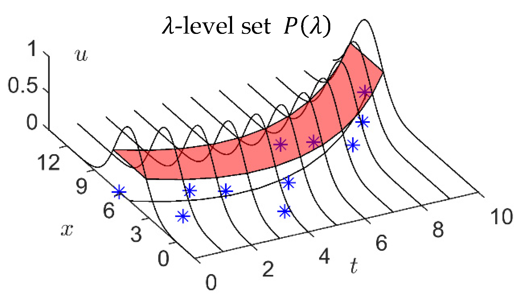
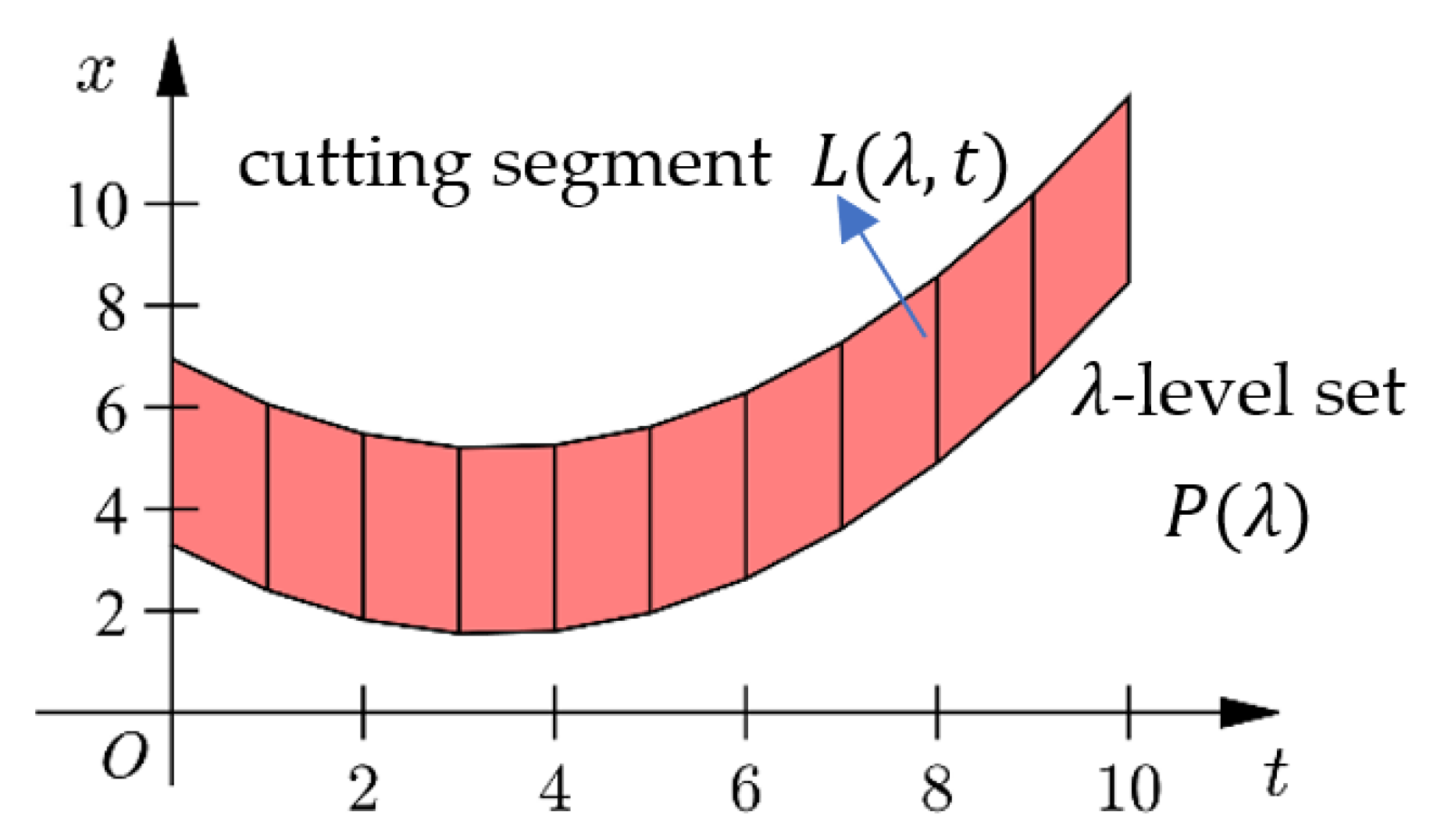
As shown in Figure 6, cut the $\lambda$-level set $P\left(\lambda \right)$ at $t=t_0$, we get a cutting segment $L\left(\lambda ,t_0\right)$:

$$L\left(\lambda ,t_0\right)=\left\{\left(t,x\right)|t=t_0,\left(t,x\right)\in P\left(\lambda \right)\right\},$$

(19)

which is a one-dimensional closed interval.

According to Equation (1), the Hausdorff distance of two cutting segments $L_1\left(\lambda ,t\right)$ and $L_2\left(\lambda ,t\right)$ at time $t$ is:

$$d\left(L_1\left(\lambda ,t\right), L_2\left(\lambda ,t\right)\right)=\max \left\{\underset{x\in L_1}{\sup }\underset{y\in L_2}{\inf }d\left(x,y\right), \underset{y\in L_2}{\sup }\underset{x\in L_1}{\inf }d\left(x,y\right)\right\}.$$

(20)

Then, the distance between $P_1\left(\lambda \right)$ and $P_2\left(\lambda \right)$ can be regarded as the sum of the distances of all these cutting segment pairs at all $t^{\prime }s$, that is:

$$d\left(P_1\left(\lambda \right),P_2\left(\lambda \right)\right)={\int }_0^{\tau }d\left(L_1\left(\lambda ,t\right), L_2\left(\lambda ,t\right)\right)\mathrm{d}t.$$

(21)

In this way, the distance of two PFIGs can be found by substituting Equation (21) to Equation (17). The distance of any different type of PFIGs can be calculated when the corresponding membership function $P\left(\left(t,x\right);\mathit{\beta },\tau ,\mathit{\gamma }\right)$ in Equation (13) is selected. In particular, the distance of two Gaussian PFIGs have the following expression.

Theorem 2.

(Distance of GPFIGs): the Hausdorff distance of two GPFIGs, namely $G_{p1}\left({\mathit{\beta }}_1,{\sigma }_1,\tau \right)$ and $G_{p2}\left({\mathit{\beta }}_2,{\sigma }_2,\tau \right)$, can be written as the area between their center lines $f_1\left(t,{\mathit{\beta }}_1\right)$ and $f_2\left(t,{\mathit{\beta }}_2\right)$, and a term proportional to the difference of ${\sigma }_1$ and ${\sigma }_2$, that is:

$$d\left(G_{p1},G_{p2}\right)={\int }_0^{\tau }\left|{\mu }_1\left(t,{\mathit{\beta }}_1\right)-{\mu }_2\left(t,{\mathit{\beta }}_2\right)\right|\mathrm{d}t+\frac{\sqrt{2\pi }\left|{\sigma }_1-{\sigma }_2\right|}{2}\tau ,$$

(22)

where $\mu \left(t,\mathit{\beta }\right)=f\left(t,\mathit{\beta }\right)$ is the center line of the GPFIG.

Proof. 

According to Equation (14), the $\lambda$-level set of GPFIG $G_p\left(\mathit{\beta },\sigma ,\tau \right)$ can be written as:

$$\begin{array}{c}P\left(\lambda \right)=\left\{\left(t,x\right)|P\left(\left(t,x\right);\mathit{\beta },\tau ,\mathit{\gamma }\right)\ge \lambda \right\}\\ \hspace{1em}\hspace{1em}\hspace{1em}\hspace{1em}=\left\{\left(t,x\right)|G_r^{-}\le x\le G_r^{+},0\le t\le \tau \right\},\end{array}$$

where $G_{\lambda }^{-}=\mu \left(t,\mathit{\beta }\right)-\sqrt{2\ln \left(1/\lambda \right)}\sigma$, and $G_{\lambda }^{+}=\mu \left(t,\mathit{\beta }\right)+\sqrt{2\ln \left(1/\lambda \right)}\sigma$. By Equation (19), the cutting segment of $P\left(\lambda \right)$ at time $t$ can be written as $L\left(\lambda ,t\right)=\left[G_{\lambda }^{-},G_{\lambda }^{+}\right]$. Substitute it into Equations (20) and (21) and we can get the following distance metric for $\lambda$-level sets $P_1\left(\lambda \right)$ and $P_2\left(\lambda \right)$.

$$\begin{array}{cc}d\left(P_1\left(\lambda \right),P_2\left(\lambda \right)\right)& ={{\displaystyle \int }}_0^{\tau }d\left(L_1\left(\lambda ,t\right), L_2\left(\lambda ,t\right)\right)dt\\ & ={{\displaystyle \int }}_0^{\tau }\left(\left|{\mu }_1\left(t,{\mathit{\beta }}_1\right)-{\mu }_2\left(t,{\mathit{\beta }}_2\right)\right|+\left|\sqrt{2\ln \left(\frac{1}{\lambda }\right)}{\sigma }_1-\sqrt{2\ln \left(\frac{1}{\lambda }\right)}{\sigma }_2\right|\right)\mathrm{d}t\\ & ={{\displaystyle \int }}_0^{\tau }\left|{\mu }_1\left(t,{\mathit{\beta }}_1\right)-{\mu }_2\left(t,{\mathit{\beta }}_2\right)\right|\mathrm{d}t+\sqrt{2\ln \left(\frac{1}{\lambda }\right)}\left|{\sigma }_1-{\sigma }_2\right|\tau .\end{array}$$

Substitute it into Equation (17) and the distance between $G_{p1}\left({\mathit{\beta }}_1,{\sigma }_1,\tau \right)$ and $G_{p2}\left({\mathit{\beta }}_2,{\sigma }_2,\tau \right)$ can be written as:

$$\begin{array}{cc}d\left(G_{p1},G_{p2}\right)& ={{\displaystyle \int }}_0^{1}d\left(P_1\left(\lambda \right),P_2\left(\lambda \right)\right)\mathrm{d}\lambda \\ & ={{\displaystyle \int }}_0^1\left({{\displaystyle \int }}_0^1\left|{\mu }_1\left(t,{\mathit{\beta }}_1\right)-{\mu }_2\left(t,{\mathit{\beta }}_2\right)\right|\mathrm{d}t+\sqrt{2\ln \left(\frac{1}{\lambda }\right)}\left|{\sigma }_1-{\sigma }_2\right|\tau \right)\mathrm{d}\lambda \\ & ={{\displaystyle \int }}_0^1\left|{\mu }_1\left(t,{\mathit{\beta }}_1\right)-{\mu }_2\left(t,{\mathit{\beta }}_2\right)\right|dt+\frac{\sqrt{2\pi }\tau }{2}\left|{\sigma }_1-{\sigma }_2\right|.\end{array}$$

□

Obviously, the first term of Equation (22) is the integral of the distance difference between two center lines $f_1\left(t,{\mathit{\beta }}_1\right)$ and $f_2\left(t,{\mathit{\beta }}_2\right)$ in $\left[0,\tau \right]$, which represents the distance caused by the center lines. As illustrated in Figure 7, the geometric meaning of this term is the area between the two center lines. The second term is $\sqrt{2\pi }\tau /2$ times of $\left|{\sigma }_1-{\sigma }_2\right|$, which represents the distance caused by data deviations. Therefore, the distance between two GPFIGs is determined by their center lines on the one hand, and the data deviations on the other. This is consistent with our intuition.

When PFIGs degenerate into LFIGs, the distance given by Equation (22) is consistent with the distance of LFIGs given in [29], i.e.,

$$d\left(G_{p1}\left({\mathit{\beta }}_1,{\sigma }_1,\tau \right),G_{p2}\left({\mathit{\beta }}_2,{\sigma }_2,\tau \right)\right)=\{\begin{array}{c}\frac{1}{2}{\tau }^2\Delta {\beta }_1+\tau \Delta {\beta }_0+\frac{\sqrt{2\pi }\tau }{2}\Delta \sigma , \mathrm{if} t^{*}<0,\\ \frac{\mathsf{\Delta }{\beta }_0{}^2}{2\mathsf{\Delta }{\beta }_1}+\frac{{\left(\mathsf{\Delta }{\beta }_0-\tau \mathsf{\Delta }{\beta }_1\right)}^2}{2\mathsf{\Delta }k}+\frac{\sqrt{2\pi }\tau }{2}\Delta \sigma , \mathrm{if} t^{*}\in \left[0,\tau \right],\\ -\frac{1}{2}{\tau }^2\Delta {\beta }_1+\tau \Delta {\beta }_0+\frac{\sqrt{2\pi }\tau }{2}\Delta \sigma , \mathrm{if} t^{*}>\tau ,\end{array}$$

where ${\mathit{\beta }}_1=\left({\beta }_{10},{\beta }_{11}\right), {\mathit{\beta }}_2=\left({\beta }_{20},{\beta }_{21}\right)$, and $f\left(t,{\mathit{\beta }}_1\right)={\beta }_{10}+{\beta }_{11}t,f\left(t,{\mathit{\beta }}_2\right)={\beta }_{20}+{\beta }_{21}t$ are the center lines of the two LFIGs, respectively. $\mathsf{\Delta }{\beta }_0=\left|{\beta }_{10}-{\beta }_{20}\right|$, $\mathsf{\Delta }{\beta }_1=\left|{\beta }_{11}-{\beta }_{21}\right|$, and $t^{*}=-\left({\beta }_{10}-{\beta }_{20}\right)/\left({\beta }_{11}-{\beta }_{21}\right)$ represents the intersection of the two center lines. $\mathsf{\Delta }\sigma =\left|{\sigma }_1-{\sigma }_2\right|$ is the difference of two data deviations.

4. Granular Time Series Prediction Method Based on Fuzzy Inference

4.1. Granule Based Fuzzy Inference

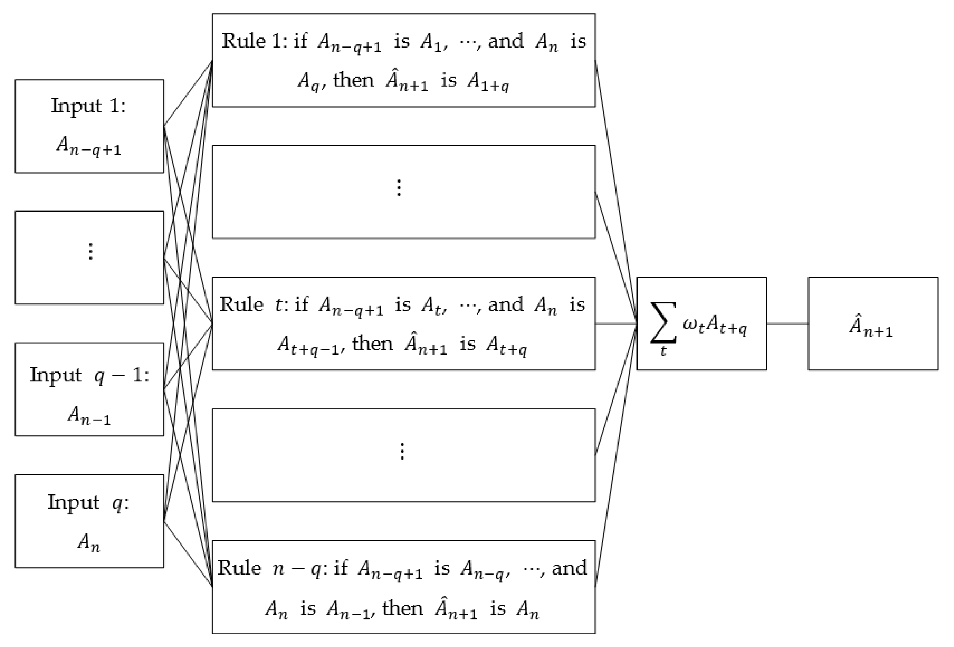
Given a time series $\mathit{y}=\left\{\left(t,y_t\right),t=1,2,\cdots ,N\right\}$, divide it into $n$ consecutive time windows, and then construct an FIG on each time window, and we can obtain a granular time series $\left\{A_1,A_2,\cdots ,A_n\right\}$. Such a granular time series can induce a fuzzy inference system (FIS) by the following way.

Select $q+1$ consecutive FIGs: $A_t, A_{t+1}, \cdots , A_{t+q-1},A_{t+q}$, and take the first $q$ FIGs as the antecedents of a fuzzy rule, and the last one as the consequent, then these $q+1$ FIGs imply a $q$-input 1-output fuzzy rule:

$$\mathrm{Rule}t: A_t,A_{t+1},\cdots ,A_{t+q-1}\to A_{t+q}.$$

A time series containing $n$ FIGs can form a total of $n-q$ rules. These rules constitute the rule base of the FIS.

As shown in Figure 8, when we use the last $q$ FIGs $A_{n-q+1},\cdots ,A_{n-1},A_n$ of this granular time series as the inputs, then the output of the FIS, namely ${\widehat{A}}_{n+1}$, can be used to predicted the future values of the original time series. Similar to the process of a Mamdani-type FIS, ${\widehat{A}}_{n+1}$ can be written as a linear combination of all the consequents of the rules, that is:

$${\widehat{A}}_{n+1}={\displaystyle \sum }_{t=1}^{n-q}{\omega }_t{A}_{t+q},$$

(23)

where ${\omega }_t$ is the weight of rule $t$, which can be measured by the Hausdorff distance between the FIS’ inputs $A_{n-q+1},\cdots ,A_{n-1},A_n$, and the antecedents of the $t$-th rule, $A_t, \cdots , A_{t+q-2}, A_{t+q-1}$. That is, ${\omega }_t$ can be written as:

$${\omega }_t=\frac{1}{D\left(A_{n-q+1},A_t\right)}\frac{1}{D\left(A_{n-q+2},A_{t+1}\right)}\cdots \frac{1}{D\left(A_{n-1},A_{t+q-1}\right)}, t=1,2,\cdots ,n-q.$$

Normalize these weights, then ${\widehat{A}}_{n+1}$ can be computed from the granular time series by Equation (23).

After obtaining a future FIG (data) ${\widehat{A}}_{n+1}$, it is incorporated into the original time series to form a new time series $\left\{A_1,A_2,\cdots ,A_n,{\widehat{A}}_{n+1}\right\}$ to predict the next FIG (data) ${\widehat{A}}_{n+2}$. Through this closed loop forecasting process, we can predict the values of any length in the future by using the previous predictions as the input. Closed loop forecasting allows us to predict an arbitrary number of time steps, but this can easily lead to large errors because the previous predictions are not the true values during the forecasting process, and the forecasting errors from a previous process can cumulatively affect the subsequent forecasting processes.

4.2. Flow Chart of the Proposed Algorithm

The pseudo-code of the time series prediction algorithm combining FIS and GPFIGs is given in Algorithm 1 as follows:

Algorithm 1: Time series prediction algorithm based on FIS and GPFIGs.

Input: A numerical time series $\mathit{y}=\left\{\left(t,y_t\right),t=1,2,\cdots ,N\right\}$ of length $N$; the granularity (length of time window) $\tau$ and the polynomial order $p$ of PFIG. Number of antecedents $q$ of the fuzzy rules in the FIS. Output: $\mathrm{the}\mathrm{next}\mathrm{FIG}{\widehat{G}}_{p,n+1}$.

(1) $\mathrm{Delete}\mathrm{the}\mathrm{first}N-\mathrm{mod}\left(N,\tau \right)$$\mathrm{elements},\mathrm{i}.\mathrm{e}.,\mathrm{let}\mathit{y}=\mathit{y}\left(N-\mathrm{mod}\left(N,\tau \right):\mathrm{end}\right);$ (2) $\mathrm{Determine}\mathrm{the}\mathrm{length}\mathrm{of}\mathrm{granular}\mathrm{time}\mathrm{series},\mathrm{i}.\mathrm{e}.,\mathrm{let}n=\mathrm{length}\left(y\right)/\tau ;$ (3) $\mathrm{For}i=1:n$; (4) $\left[{\beta }_i,{\sigma }_i\right]=p$$\mathrm{th}-\mathrm{OrderPolynomialFitting}\left(y\left(i\tau +1:\left(i+1\right)\tau \right),p\right)$; (5) End (6) $\mathrm{Construct}\mathrm{a}\mathrm{granular}\mathrm{time}\mathrm{series}\left\{\left(i,G_{p,i}\left({\beta }_i,\tau ,{\sigma }_i\right)\right),i=1,2,\cdots ,n\right\};$ (7) $\mathrm{For}i=1:n-q$; (8) ${\omega }_i=\frac{1}{D\left(G_{p,n-q+1},G_i\right)}\cdot \frac{1}{D\left(G_{p,n-q+2},G_{i+1}\right)}\cdot \cdots \cdot \frac{1}{D\left(G_{p,n-1},G_{i+q-1}\right)};$ (9) End; (10) ${\widehat{G}}_{p,n+1}=\sum _{i=1}^{n-q}\left(\frac{{\omega }_i}{{\sum }_{t=1}^{n-q}{\omega }_t}{G}_{i+q}\right)$.

5. Experimental Research

To test the effectiveness of the perdition algorithm combining an FIS and GPFIGs (GPFIG-FIS), the forecasting results of the proposed method are compared with eight competing models in this section.

5.1. Data Description and Experimental Scheme

Three kinds of time series with a pseudo periodicity are selected for the experiment in this section. These data include: (1) the time series of the daily minimum temperature in Melbourne from 1981 to 1990 (this time series is from: https://www.kaggle.com/datasets/sayedathar11/minimum-daily-temperatures-in-melborne19811990, accessed on 15 August 2022); (2) Tetouan city power consumption time series (this time series is from: https://archive.ics.uci.edu/ml/datasets/Power+consumption+of+Tetouan+city, accessed on 15 August 2022); and (3) American Heart Association electrocardiograms (ECG) time series (this time series dataset is purchased from: https://www.ecri.org/american-heart-association-ecg-database-usb, accessed on 1 June 2020).

Two kinds of indexes, the root mean-square error (RMSE) and symmetric mean absolute percentage error (SMAPE), are used to measure the effect of the time series prediction methods:

• Root mean-square error:

$$RMSE=\sqrt{\frac{{\sum }_{t=1}^n{\left(\widehat{y}\left(t\right)-y\left(t\right)\right)}^2}{n}}.$$

• Symmetric mean absolute percentage error:

$$SMAPE=\frac{1}{n}{\displaystyle \sum }_{t=1}^n\frac{\left|\widehat{y}\left(t\right)-y\left(t\right)\right|}{\frac{1}{2}\left(\left|\widehat{y}\left(t\right)\right|+\left|y\left(t\right)\right|\right)}\times 100.$$

where $n$ indicates the number of data to be predicted, and $y\left(t\right)$ and $\widehat{y}\left(t\right)$ indicate the true and predicted values of the time series at time $t$, respectively.

The following eight prediction methods are selected for a comparison with the GPFIG-FIS method proposed in this paper, among which the first four methods are numerical prediction methods, and the last four methods are methods based on ordinary FIGs and FIS:

• AR($q$): Numerical $q$-order auto regressive model (auto regressive, AR):

$$y\left(t\right)={\varphi }_{1}y\left(t-1\right)+{\varphi }_{2}y\left(t-2\right)+\cdots +{\varphi }_{q}y\left(t-q\right)+{ϵ}_t,$$

where ${\varphi }_1,{\varphi }_2,\cdots , {\varphi }_q$ can be calculated from the training data by linear regression.

• NAR($q$): the $q$-order NAR is a $q$-input 1-output feedforward network, whose input is a vector $x_t\stackrel{\mathrm{def}}{=}\left\{y\left(t-1\right),y\left(t-2\right),\dots ,y\left(t-q\right)\right\}$ consisting of $q$ data before time $t$ in the given training sequence, and output is the datum in time $t$, $y_t=y\left(t\right)$. The NAR uses a sigmoid transfer function in the hidden layer and a linear transfer function in the output layer. The number of hidden neurons as well as the number of hidden layers is set to 10.
• SVR($q$): numerical $q$-order support vector machine regress model (support vector regress, SVR) [39]:

$$\widehat{y}\left(t\right)=w_{1}y\left(t-1\right)+w_{2}y\left(t-2\right)+\cdots +w_{q}y\left(t-q\right)+b,$$

where parameters $w=\left(w_1,w_2,\cdots ,w_q\right)$ and $b$ are determined by the following support vector machine regression model:

$$\underset{\mathrm{w}}{\min }\frac{1}{2}{w}^{T}w+C\frac{1}{l}{\displaystyle \sum }_{t=1}^l\left({\xi }_t+{\xi }_t^{*}\right),$$

$$s.t. \left(w^T{x}_t+b\right)-y_t\le ϵ+{\xi }_t,$$

$$y_t-\left(w^T{x}_t+b\right)\le ϵ+{\xi }_t^{*},$$

$${\xi }_t, {\xi }_t^{*}\ge 0,$$

where $l$ is the number of training samples, $x_t$ and $y_t$ are the same as in NAR($q$);

• LSTM: a sequence-to-sequence regression LSTM network, where the responses are the training sequences with values shifted by one time step. The LSTM updates the cell and hidden states using the hyperbolic tangent function and uses the sigmoid function as the gate activation function. The number of hidden units is set to 128.
• IFIG-FIS: the FIS prediction method based on the IFIG. Equations (4) and (5) are used to granulate the time series, and the FIS with $q$-input is used for the prediction.
• TFIG-FIS: the FIS prediction method based on the TFIG. Equations (7) and (8) are used to granulate the time series, and the FIS with $q$-input is used for the prediction.
• GFIG-FIS: the FIS prediction method based on the GFIG. The average and standard deviation of the corresponding window data are used as the parameters in constructing the GFIG, and the FIS with $q$-input is used for the prediction.
• LIFG-FIS: the FIS prediction method based on the LFIG. The linear regression line and the estimate of the error variance are used as the parameters in constructing the LIFG, and the FIS with $q$-input is used for the prediction.

5.2. The Experimental Results

5.2.1. Daily Minimum Temperature Dataset

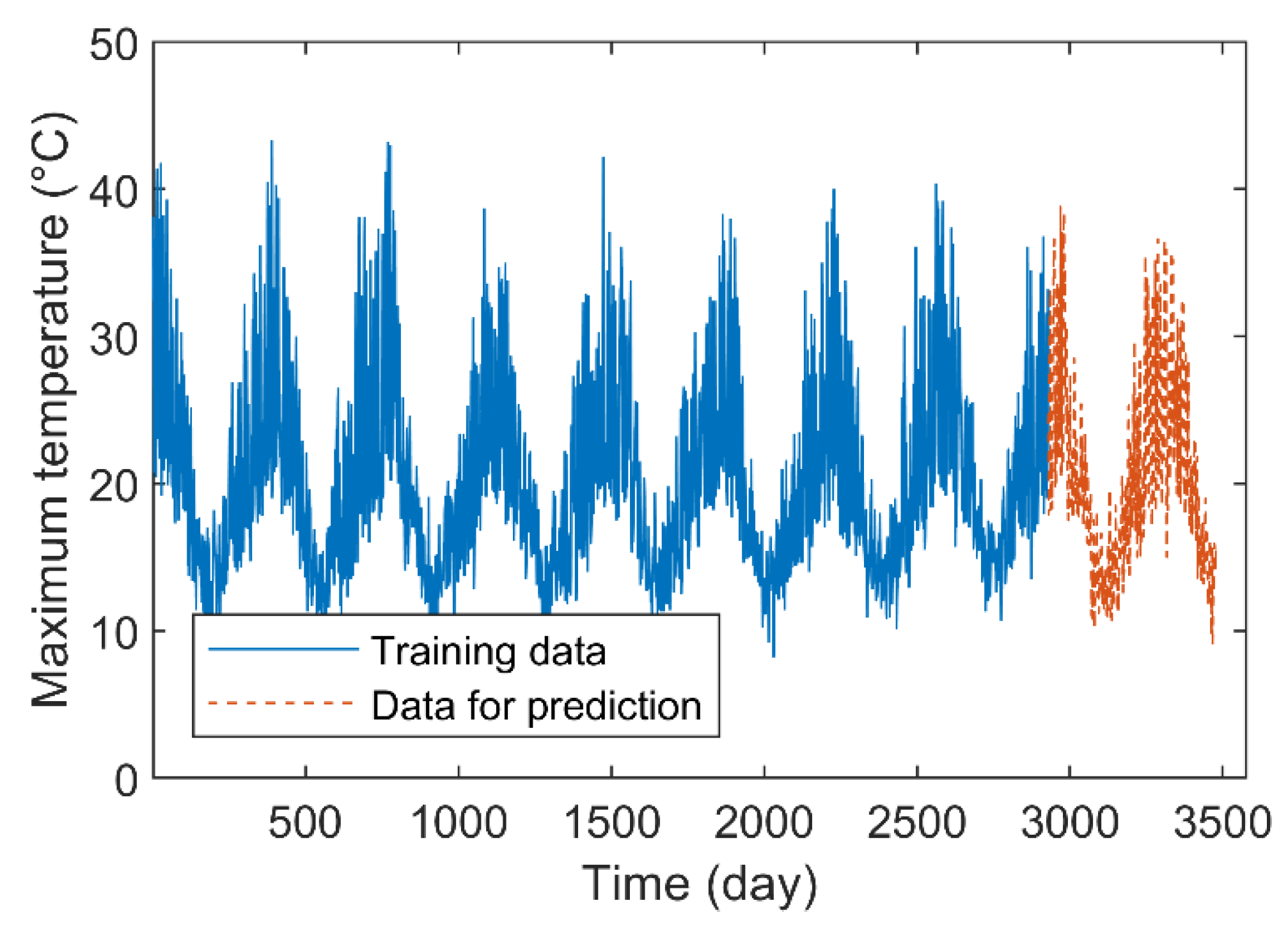
The time series of daily maximum temperature in Melbourne City from 1981 to 1990 is shown in Figure 9. The time series contains a total of 3650 data, and the first 2928 data are selected as the training samples to predict the daily maximum temperature for the next 183, 366, and 549 days (i.e., days after 2928).

For each prediction method, the number of FIS input $q$ is set to three. Since this time series has a natural time cycle, in constructing the granular time series, the size of the time window is set to 183 days, which is about half a year. Additionally, the order of the GPFIG is set as three.

Table 1. Comparison of the prediction indexes of daily minimum temperature.

Index	Time (Day)	AR	NAR	SVR	LSTM	IFIG-FIS	TFIG-FIS	GFIG-FIS	LFIG-FIS	GPFIG-FIS
RMSE	2929–3112	9.83	6.79	6.49	4.30	8.76	6.67	6.45	4.44	4.19
	2929–3295	14.76	7.01	6.54	4.25	7.57	6.39	6.18	4.27	4.14
	2929–3478	17.23	6.83	6.4	4.25	7.86	6.31	6.11	4.19	4.04
SMAPE	2929–3112	42.02	27.58	24.74	14.32	28.14	21.67	22.38	14.66	14.11
	2929–3295	62.34	30.63	27.23	15.51	24.48	21.27	21.97	14.71	14.48
	2929–3478	74.18	29.9	26.73	14.87	25.85	21.74	22.47	14.66	14.28

Note: a value in bold font indicates that the corresponding method achieves the best index among all the methods.

shows the RMSE and SMAPE indexes by the GPFIG-FIS and other methods for a long-term forecasting.

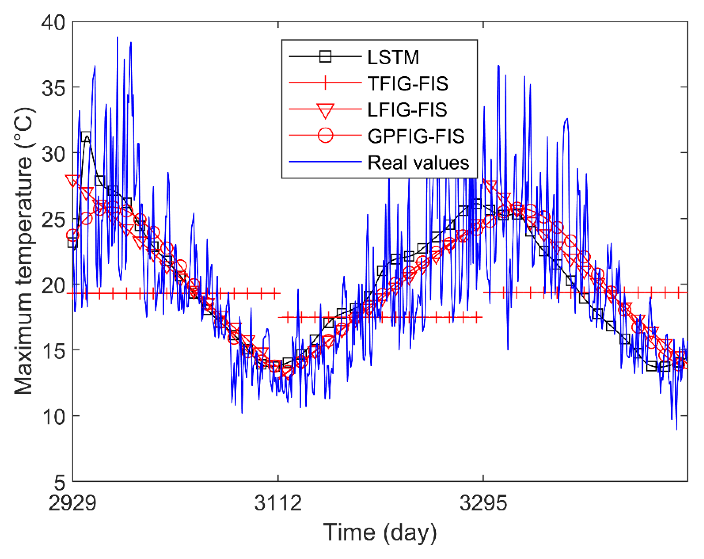
For brevity, Figure 10 shows the predicted values of several prediction methods with better prediction results. It can be found that compared with the numerical prediction methods, the LFIG-FIS and GPFIG-FIG get better prediction results. Because of the length of the time window, which is about half a year, it has a clear meaning in this experiment, the FIGs constructed by the LFIG-FIS and GPFIG-FIG can reflect the main characteristics of the data in each time window very well, which is beneficial to eliminate the influence of random noises in this time series. When these FIGs are regarded as linguistic variables to construct fuzzy inference rules, a reasonable FIS can be obtained. However, since numerical prediction methods are easily disturbed by noise, they cannot get accurate results for a long-term prediction.

Note that the time series used in this experiment has a clear increasing or decreasing trend in each time window. Because of this, both the LFIG-FIS and GPFIG-FIS that contain trend parameters could accurately reflect these changing trends. Therefore, compared with the other FIG-based prediction methods, the LFIG-FIS and GPFIG-FIS can get better prediction results. Among them, the GPFIG-FIS is slightly better than the LFIG-FIS because it can more accurately reflect the changing trends in each time window.

5.2.2. Power Consumption Time Series

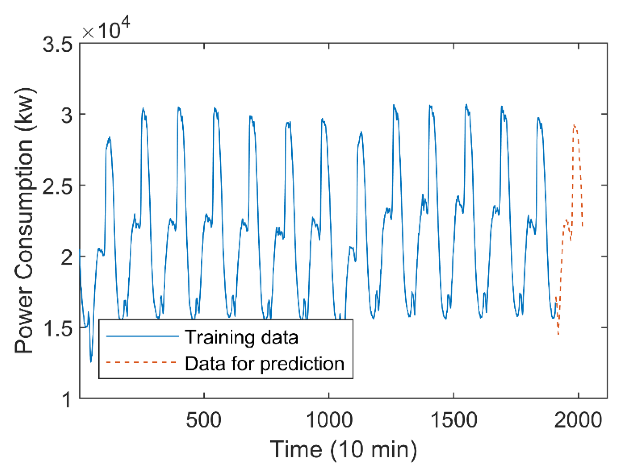
The average power consumption data of the three urban areas every 10 min are collected in the two weeks from 16 to 30 December 2017 in Tetuan, Morocco. As shown in Figure 11, this time series contains 2016 data, and the previous 1920 data are used as the training data set, to predict the last 96 data.

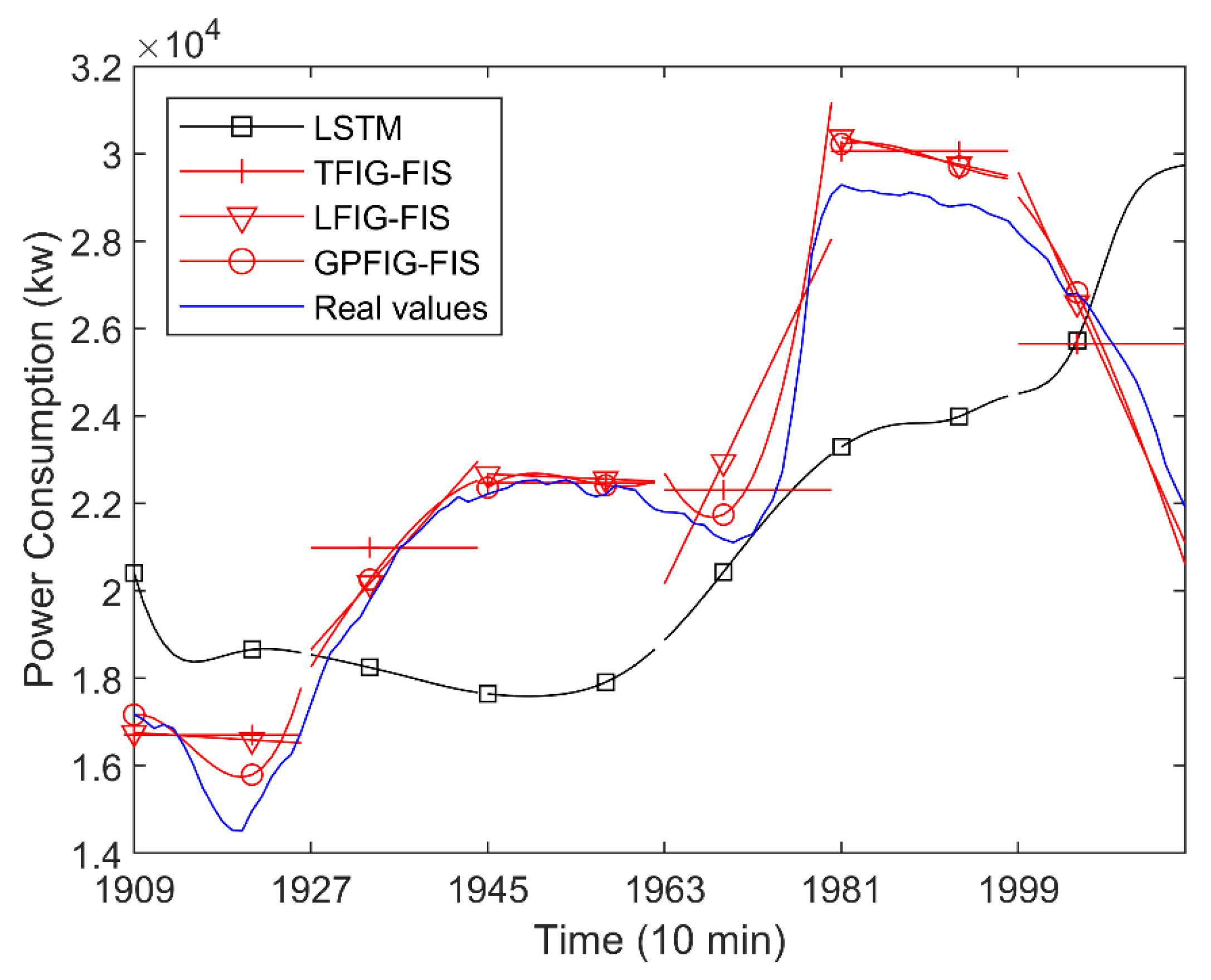
Set the number of FIS input $q=3$ for the various methods. The length of the time window is set as 16, about one ninth of a day, in constructing various kinds of FIGs. Additionally, the polynomial order of the PFIG is set as three.

Table 2. Comparison of the prediction indexes of electricity consumption in Tetuan.

Index	Time (10 min)	AR	NAR	SVR	LSTM	IFIG-FIS	TFIG-FIS	GFIG-FIS	LFIG-FIS	GPFIG-FIS
RMSE	1909–1926	3479	3128	5556	2934	1630	1155	1033	1087	692
	1927–1944	2800	2749	4130	2909	1647	1394	1306	854	565
	1945–1962	3030	3896	3415	3522	1394	1146	1077	718	482
	1963–1980	3803	4765	3347	3343	1790	1701	1676	1141	691
	1981–1998	6020	6815	4504	3755	1687	1603	1547	1101	744
	1999–2016	6500	7273	4526	3828	1823	1657	1617	1065	754
SMAPE	1909–1926	19.11	16.68	32.89	16.87	8.27	5.55	5.12	5.17	3.36
	1927–1944	13.77	13.35	20.14	14.79	7.64	6.22	5.99	3.68	2.62
	1945–1962	14.92	18.04	14.94	17.29	6.12	4.42	4.33	2.88	2.07
	1963–1980	16.89	21.15	13.29	15.36	7.08	5.48	6.38	4.21	2.7
	1981–1998	22.99	27.07	17.05	16.61	6.66	5.33	5.81	4.16	2.95
	1999–2016	25.47	29.38	17.38	16.65	6.97	5.68	6.11	4.08	3.02

Note: a value in bold font indicates that the corresponding method achieves the best result among all the methods.

shows the RMSE and SMAPE indexes of various methods in predicting the data in the last six time windows (96 points altogether).

For brevity, Figure 12 shows the predicted values of four prediction methods with better prediction results. Figure 12 and Table 2 show that, compared with the numerical prediction methods, the FIG-based prediction methods, namely the IFIG-FIS, TFIG-FIG, LFIG-FIS, and GPFIG-FIG can have more accurate prediction results, among which the LFIG- and GPFIG-based methods can reflect the time-varying trend very well. Therefore, they have better RMSE and SMAPE indexes when dealing with long-term prediction. In predicting the values of different time periods in the future, the GPFIG-FIS always has the best RSME and SMAPE indexes. A reason for this result is that, compared with the previous experiment, the power consumption time series display more complex trend changes in each time window, and the GPFIG with a high-order polynomial center line can better describe these changes. Consequently, the prediction indexes of the GPFIG-FIS are also significantly better than other methods such as the LFIG-FIS.

5.2.3. American Heart Association Electrocardiogram Time Series

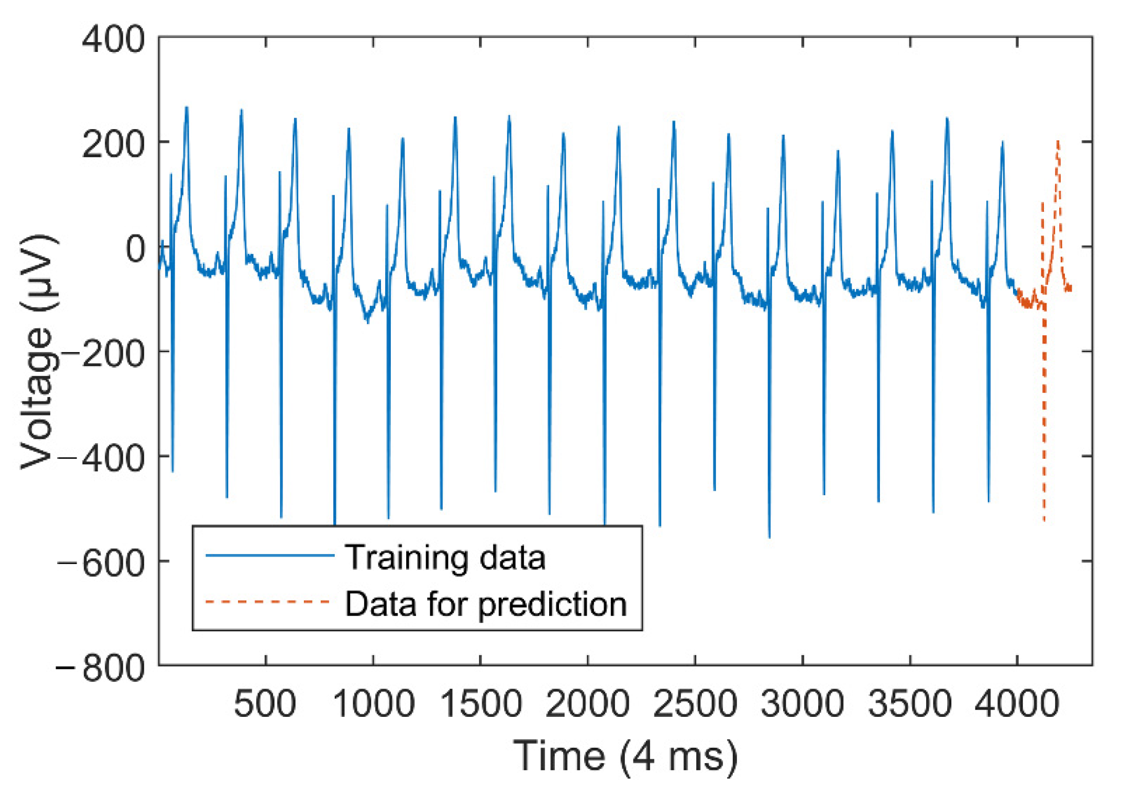
The American Heart Association (AHA) ECG datasets collect voltage values at a sampling rate of 250 Hz. A complete ECG waveform contains about 250 sampling points. So, when constructing various FIGs, the length of the time window is set as 25, which is about one-tenth of a whole waveform. Figure 13 plots a time series containing 4250 sampling points. The first 4000 sampling points (including about 16 waveforms) are used as the training set to predict the last 250 sampling points (about 1 waveform).

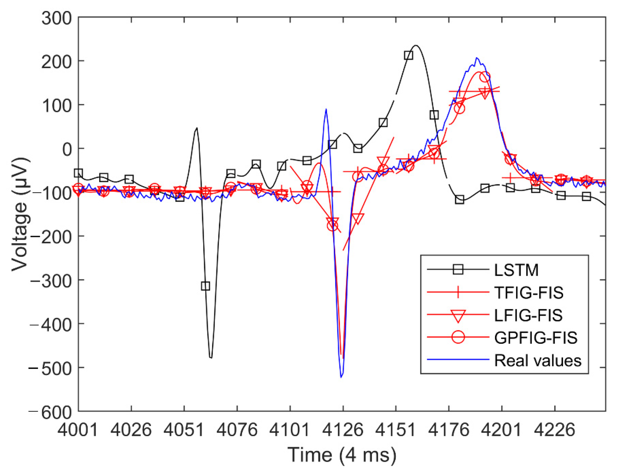
Set the number of the FIS input $q=10$ for each prediction method. Due to the complexity of the ECG waveform, the polynomial order of the PFIG is set as four.

Table 3. Comparison of the prediction indexes of ECG time series.

Index	Time (4 ms)	AR	NAR	SVR	LSTM	IFIG-FIS	TFIG-FIS	GFIG-FIS	LFIG-FIS	GPFIG-FIS
RMSE	4001–4025	87.91	22.74	41.06	26.83	7.33	7.43	7.7	7.2	7.96
	4026–4050	99.24	40.4	48.48	22.58	8.61	10.67	13.03	12.01	11.84
	4051–4075	102.95	52.92	51	94.60	12.23	12.34	13.82	12.93	12.1
	4076–4100	102.58	67.47	50.23	85.65	12.68	12.85	14.2	12.27	11.31
	4101–4125	124.51	129.95	83.39	114.43	70.03	64.81	64.07	59.72	30.74
	4126–4150	131.99	164.89	93.48	130.28	107.32	80.48	76.25	65.06	29.18
	4151–4175	122.86	163.78	89.79	139.07	100.47	76.09	72.11	60.88	28.41
	4176–4200	127.1	154.01	111.27	157.61	95.37	73.1	69.92	60.01	28.8
	4201–4225	121.25	160.38	105.42	149.67	93.44	69.98	66.71	56.75	27.4
	4226–4250	117.79	169.45	100.35	142.36	88.9	66.46	63.34	53.9	26.14
SMAPE	4001–4025	95.44	22.32	45.72	28.70	6.48	6.75	6.36	6.31	7.43
	4026–4050	106.77	39.06	52.28	22.25	7.59	9.55	11.5	10.69	10.63
	4051–4075	111.88	52.56	55.11	59.09	10.77	11.42	12.75	11.87	11.2
	4076–4100	113.48	67.23	54.62	56.81	11.84	12.38	13.52	11.25	10.38
	4101–4125	114.54	91.74	60.64	66.26	25.84	23.55	24.93	27.62	19.71
	4126–4150	113.47	127.12	56.93	81.95	70.16	26.25	32.58	33.95	19.31
	4151–4175	106.49	164.82	67.18	150.81	71.01	31.95	37.2	35.64	23.8
	4176–4200	109.68	149.17	81.82	160.37	67.17	32.85	37.63	36.3	24.15
	4201–4225	107.33	174.87	79.45	152.83	73.07	37.05	40.11	35.21	23.45
	4226–4250	107.68	190.28	74.94	141.83	68.52	34.43	36.93	32.6	22.05

Note: A value in bold font indicates that the corresponding method achieves the best result among all the methods.

shows the RMSE and SMAPE indexes of the various prediction methods.

For brevity, Figure 14 shows the predicted values of several prediction methods with better results. It can be found from Figure 14 and Table 3 that, compared with numerical prediction methods, the prediction methods based on the FIG and FIS have better prediction results.

The changing trends of the ECG time series are more complex than previous experiments. As is shown in Figure 14, this time series is very stable in the first four time windows, and then there are sharp fluctuations from the fifth time window. Correspondingly, in the first four time windows, the RSME and SMAPE indexes of the GPFIG-FIS are almost the same with those of the other FIS-based methods. However, from the fifth time window, the predictive indexes of the GPFIG-FIS are significantly better than the other prediction methods. The main reason for this result is that GPFIG can accurately describe the changing trends in the ECG data through its high-order polynomial center line. In summary, for the ECG time series with complex changing trends, the GPFIG-FIS method can obtain better long-term prediction results.

6. Summary

The PFIGs can accurately describe the key time-varying nonlinear trends of the time series, and thus are a suitable type of FIGs in granulating a time series. A PFIG has three parameters, namely the length of the time window, the centerline of the adjustable order polynomial, and the degree of the data deviation, which have a good interpretability and are easy to understand.

The distance metric of PFIGs is derived theoretically. It shows that the distance of two Gaussian PFIGs can be reasonably interpreted as the sum of the area between their central polynomial lines, and the difference in their data deviation degrees, which has a good geometric meaning.

This paper also designs a fuzzy inference prediction method based on the GPFIG and their distance metric to verify the effectiveness of the proposed GPFIG. The experiments show that for those time series with pseudo periods, the proposed GPFIG-FIS method can achieve better prediction results compared with some numerical prediction methods such as the AR, NAR, SVR and LSTM, and some fuzzy inference methods based on other types of FIG. This conclusion shows that the proposed GPFIG has a good practicability.

The PFIG time series constructed in this paper is composed of several PFIGs of an equal granularity. A question associated with the granulation method in this paper is how to choose the optimal granularity of these PFIGs. Without sufficient periodic knowledge of the time series to be transformed in advance, it may be difficult to determine the best granularity.

A further generalization of the PFIG can improve the ability of the granular time series in representing the complicated time series. How to use this new PFIG to deal with a real-world prediction problem may be a subject of future research.

References

- Zhang, H.; Nguyen, H.; Bui, X.-N.; Biswajeet, P.; Mai, N.-L.; Vu, D.A. Proposing two novel hybrid intelligence models for forecasting copper price based on extreme learning machine and meta-heuristic algorithms. Resour. Policy 2021, 73, 102195. [Google Scholar] [CrossRef]
- Wang, H.; Luo, C.; Wang, X. Synchronization and identification of nonlinear systems by using a novel self-evolving interval type-2 fuzzy LSTM-neural network. Eng. Appl. Artif. Intell. 2019, 81, 79–93. [Google Scholar] [CrossRef]
- Jiang, P.; Yang, H.; Li, H.; Wang, Y. A developed hybrid forecasting system for energy consumption structure forecasting based on fuzzy time series and information granularity. Energy 2021, 219, 119599. [Google Scholar] [CrossRef]
- Box, G.; Jenkins, G.; Reinsel, G. Forecasting and Control, 4th ed.; Time Series Analysis; John Wiley & Sons: New York, NY, USA, 2008. [Google Scholar]
- Moon, J.; Hossain, M.B.; Chon, K. AR and ARMA model order selection for time-series modeling with ImageNet classification. Signal Process. 2021, 183, 108026. [Google Scholar] [CrossRef]
- Xian, H.; Che, J. Unified whale optimization algorithm based multi-kernel SVR ensemble learning for wind speed forecasting. Appl. Soft Comput. 2022, 130, 109690. [Google Scholar] [CrossRef]
- Yoon, H.; Hyun, Y.; Ha, K.; Lee, K.-K.; Kim, G.-B. A method to improve the stability and accuracy of ANN- and SVM-based time series models for long-term groundwater level predictions. Comput. Geosci. 2016, 90, 144–155. [Google Scholar] [CrossRef]
- Sunayana; Kumar, S.; Kumar, R. Forecasting of municipal solid waste generation using non-linear autoregressive (NAR) neural models. Waste Manag. 2021, 121, 206–214. [Google Scholar] [CrossRef] [PubMed]
- Bandara, K.; Bergmeir, C.; Smyl, S. Forecasting across time series databases using recurrent neural networks on groups of similar series: A clustering approach. Expert Syst. Appl. 2020, 140, 112896. [Google Scholar] [CrossRef] [Green Version]
- Arsov, M.; Zdravevski, E.; Lameski, P.; Corizzo, R.; Koteli, N.; Gramatikov, S.; Mitreski, K.; Trajkovik, V. Multi-Horizon Air Pollution Forecasting with Deep Neural Networks. Sensors 2021, 21, 1235. [Google Scholar] [CrossRef]
- Livieris, I.E.; Pintelas, E.; Pintelas, P. A CNN–LSTM model for gold price time-series forecasting. Neural Comput. Appl. 2020, 32, 17351–17360. [Google Scholar] [CrossRef]
- Jin, X.; Yu, X.; Wang, X.; Bai, Y.; Su, T.; Kong, J. Prediction for Time Series with CNN and LSTM. In Proceedings of the 11th International Conference on Modelling, Identification and Control (ICMIC2019), Tianjin, China, 4 December 2019; Wang, R., Chen, Z., Zhang, W., Zhu, Q., Eds.; Springer: Singapore, 2020; p. 59. [Google Scholar]
- Jilani, T.A.; Burney, S.M.A. M-factor high order fuzzy time series forecasting for road accident data: Analysis and design of intelligent systems using soft computing techniques. Adv. Soft Comput. 2007, 41, 246–254. [Google Scholar]
- Wang, L.; Xue, T.; Wang, H.; Liu, Z. Research on stock index forecasting based on recurrent neural network. J. Zhejiang Univ. Technol. 2019, 47, 186–191. [Google Scholar]
- Wang, X.; Wu, J.; Liu, C.; Yang, H.; Niu, W. Exploring LSTM based recurrent neural network for failure time series prediction. J. Beijing Univ. Aeronaut. Astronaut. 2018, 44, 772–784. [Google Scholar]
- Tang, Y.; Yu, F.; Pedrycz, W.; Yang, X.; Wang, J.; Liu, S. Building trend fuzzy granulation based LSTM recurrent neural network for long-term time series forecasting. IEEE Trans. Fuzzy Syst. 2022, 30, 1599–1613. [Google Scholar] [CrossRef]
- Cheng, R.; Yu, J.; Zhang, M.; Feng, C.; Zhang, W. Short-term hybrid forecasting model of ice storage air-conditioning based on improved SVR. J. Build. Eng. 2022, 50, 104194. [Google Scholar] [CrossRef]
- Keogh, E.; Kasetty, S. On the need for time series data mining benchmarks: A survey and empirical demonstration. Data Min. Knowl. Discov. 2002, 7, 102–111. [Google Scholar]
- Zadeh, L. Advances in Fuzzy Set Theory and Applications; World Scientific Publishing: Amsterdam, The Netherlands, 1979; pp. 3–18. [Google Scholar]
- Pedrycz, W.; Vukovich, G. Abstraction and specialization of information granules. IEEE Trans. Syst. Man Cybern. Part B 2001, 31, 106–111. [Google Scholar] [CrossRef]
- Guo, J.; Lu, W.; Yang, J.; Liu, X. A rule-based granular model development for interval-valued time series. Int. J. Approx. Reason. 2021, 136, 201–222. [Google Scholar] [CrossRef]
- Ruan, J.; Wang, X.; Shi, Y. Developing fast predictors for large-scale time series using fuzzy granular support vector machines. Appl. Soft Comput. 2013, 13, 3981–4000. [Google Scholar] [CrossRef]
- Zhou, Y.; Ren, H.; Li, Z.; Pedrycz, W. Anomaly detection based on a granular Markov model. Expert Syst. Appl. 2022, 187, 115744. [Google Scholar] [CrossRef]
- He, L.; Chen, Y.; Zhong, C.; Wu, K. Granular Elastic Network Regression with Stochastic Gradient Descent. Mathematics 2022, 10, 2628. [Google Scholar] [CrossRef]
- Hu, M.; Wang, C.; Yang, J.; Wu, Y.; Fan, J.; Jing, B. Rain Rendering and Construction of Rain Vehicle Color-24 Dataset. Mathematics 2022, 10, 3210. [Google Scholar] [CrossRef]
- Yu, F.; Pedrycz, W. The design of fuzzy information granules: Tradeoffs between specificity and experimental evidence. Appl. Soft Comput. 2009, 9, 264–273. [Google Scholar] [CrossRef]
- Pedrycz, W.; Wang, X. Designing fuzzy sets with the use of the parametric principle of justifiable granularity. IEEE Trans. Fuzzy Syst. 2016, 24, 489–496. [Google Scholar] [CrossRef]
- Dong, K. Time Series Information Granulation and Clustering Analysis Based on Granulation; Beijing Normal University: Beijing, China, 2005. [Google Scholar]
- Yang, X.; Yu, F.; Pedrycz, W. Long-term forecasting of time series based on linear fuzzy information granules and fuzzy inference system. Int. J. Approx. Reason. 2017, 81, 1–27. [Google Scholar] [CrossRef]
- Luo, C.; Song, X.; Zheng, Y. A novel forecasting model for the long-term fluctuation of time series based on polar fuzzy information granules. Inf. Sci. 2020, 512, 760–779. [Google Scholar] [CrossRef]
- Luo, C.; Wang, H. Fuzzy forecasting for long-term time series based on time-variant fuzzy information granules. Appl. Soft Comput. 2020, 88, 106046. [Google Scholar] [CrossRef]
- Tang, Y.; Yu, F. Fuzzy information granulation: Review of theory and applications. J. Beijing Norm. Univ. 2022, 58, 349–361. [Google Scholar]
- Zadeh, L.A. Fuzzy sets. Inf. Control 1965, 8, 338–353. [Google Scholar] [CrossRef] [Green Version]
- Shen, Y. Calculus for linearly correlated fuzzy number-valued functions. Fuzzy Sets Syst. 2022, 429, 101–135. [Google Scholar] [CrossRef]
- Rote, G. Computing the minimum Hausdorff distance between two point sets on a line under translation. Inf. Process. Lett. 1991, 38, 123–127. [Google Scholar] [CrossRef]
- Dubois, D.; Prade, H. Fundamentals of Fuzzy Sets; Springer: New York, NY, USA, 2000; p. 90. [Google Scholar]
- Yu, F.; Dong, K.; Chen, F.; Jiang, Y.; Zeng, W. Clustering Time Series with Granular Dynamic Time Warping Method. In Proceedings of the Clustering Time Series with Granular Dynamic Time Warping Method, Fremont, CA, USA, 2–4 November 2007; p. 393. [Google Scholar]
- Luo, C.; Yu, F.; Zeng, W. Introduction to Fuzzy Sets; Beijing Normal University Press: Beijing, China, 2019. [Google Scholar]
- Fan, R.; Chang, K.; Hsieh, C.; Wang, X.R.; Lin, C.J. LIBLINEAR: A library for large linear classification. J. Mach. Learn. Res. 2008, 9, 1871–1874. [Google Scholar]
Figure 1.
Fuzzy numbers. (a) a one-dimensional fuzzy number; (b) a two-dimensional fuzzy number.
Figure 2.
Different types of fuzzy information granules. (a) time series data; (b) interval fuzzy information granule; (c) triangular fuzzy information granule; (d) Gaussian fuzzy information granule.
Figure 3.
A linear fuzzy information granule.
Figure 4.
A Gaussian PFIG.
Figure 5.
The -level set of a PFIG.
Figure 6.
The cutting segment of the -level set in a PFIG.
Figure 7.
The area between the two center lines. (a) The area of two center lines when they have no intersection between [0,τ], (b) the area of two center lines when they have an intersection between [0,τ].
Figure 8.
Fuzzy inference system.
Figure 9.
Time series of daily maximum temperature.
Figure 10.
Daily maximum temperature forecast results.
Figure 11.
Time series of average power consumption in Tetuan.
Figure 12.
Electricity consumption forecast results of Tetuan city.
Figure 13.
Electrocardiogram time series.
Figure 14.
Electrocardiogram prediction results.