Bright Soliton Solution of the Nonlinear Schrödinger Equation: Fourier Spectrum and Fundamental Characteristics

Abstract

We derive exact analytical expressions for the spatial Fourier spectrum of the fundamental bright soliton solution for the $\left(1+1\right)$-dimensional nonlinear Schrödinger equation. Similar to a Gaussian profile, the Fourier transform for the hyperbolic secant shape is also shape-preserving. Interestingly, this associated hyperbolic secant Fourier spectrum can be represented by a convergent infinite series, which can be achieved using Mittag–Leffler’s expansion theorem. Conversely, given the expression of the series of the spectrum, we recover its closed form by employing Cauchy’s residue theorem for summation. We further confirm that the fundamental soliton indeed satisfies essential characteristics such as Parseval’s relation and the stretch-bandwidth reciprocity relationship. The fundamental bright soliton finds rich applications in nonlinear fiber optics and optical telecommunication systems.

1. Introduction

The nonlinear Schrödinger (NLS) equation is a nonlinear evolution equation for slowly varying wave packet envelopes in dispersive media. It belongs to a category of completely integrable systems or exactly solvable models of a nonlinear partial differential equation (PDE), with infinitely many conserved quantities and explicit analytical solutions [1,2]. The NLS equation finds rich applications in mathematical physics, including surface gravity waves, nonlinear optics, superconductivity, and Bose–Einstein condensates (BECs) [3,4,5].

The focus of this article is the one-dimensional focusing type of the NLS equation. The former is sometimes also written as $(1+1)$-D, where usually, there is only one dimension each in the spatial and temporal variables. Higher-dimensional models usually extend the dimension of the dispersive term. In the canonical form, the focusing $\left(1+1\right)$-D NLS equation can be expressed as the following nonlinear PDE and the subscript indicates the partial derivative with respect to the associated variable [1,6,7]:

$$i{q}_t+q_{xx}+2{\left|q\right|}^{2}q=0,\left(x,t\right)\in {\mathbb{R}}^2,q\left(x,t\right)\in \mathbb{C}.$$

(1)

This type of NLS equation is also called the cubic Schrödinger equation because of the third-order nonlinear term. In the absence of this nonlinear term, the NLS equation reduces to the linear Schrödinger equation, a comparably well-known mathematical model that is used extensively in quantum mechanics for calculating the wave function of an electron. In the context of BECs, the NLS equation is also known as the Gross–Pitaevskii equation.

In nonlinear optics, the derivation of the NLS equation employs Maxwell–Heaviside equations that unifies light, electricity, and magnetism [8,9]. In plasma physics, the method of multiple scales was utilized to derive the NLS equation for hydromagnetic waves that propagate along the magnetic field in cold plasmas [10]. The NLS equation was also derived independently around the same time in hydrodynamics for describing the propagation of wave packet envelopes [11]. Several other authors derived the NLS equation using different techniques in various physical settings, such as the Whitham–Lighthill adiabatic approximation [12], asymptotic theory for heat pulses in solids [13], the perturbation method for waves in an electron plasma system [14,15], a spectral method for deep-water waves [16], and the singular perturbation method in gravity water waves with finite depth [17].

In surface gravity waves, the independent variables $\left(x,t\right)$ represent spatial and temporal quantities, respectively, whereas in nonlinear optics, t denotes the transversal pulse propagation in space and x designates the time variable. The focusing type is indicated by the positive product of the dispersive and nonlinear coefficients, which are also known in optical pulse propagation as group-velocity dispersion and self-phase modulation, respectively. In this article, we adopt the physical interpretation from hydrodynamics for the independent variables.

The dependent variable $q\left(x,t\right)$ is a complex-valued amplitude. It describes the slowly varying envelope dynamics of the corresponding weakly nonlinear quasi-monochromatic wave packet profile. Denoted by $\eta \left(\overline{x},\overline{t}\right)$, the usual relationship with $q\left(x,t\right)$ is given by

$$\eta \left(\overline{x},\overline{t}\right)=\mathrm{Re}\left\{q\left(x,t\right)e^{i\left(k\overline{x}-\omega \overline{t}\right)}\right\},$$

where $x=\epsilon \left(\overline{x}-c_g\overline{t}\right)$ and $t={\epsilon }^2\overline{t}$, with $\epsilon \ll 1$. Here, $c_g$ denotes the group velocity, and the wavenumber k and wave frequency $\omega$ are related by the linear dispersion relationship for the corresponding medium.

The purpose of this article is to provide a step-by-step explanation for finding the physical spectrum, i.e., the spatial Fourier spectrum, of the bright soliton solution of the NLS equation. Additionally, we also demonstrated that, on the one hand, the expression for the spectrum can be expressed as a convergent infinite series using Mittag–Leffler’s expansion theorem, while on the other hand, given a series expression, it can be returned to its original closed form by an entirely different technique, albeit still utilizing a tool from complex analysis, i.e., Cauchy’s residue theorem. The term “spectrum” should not be confused with the one used in the well-known inverse scattering transform (IST) technique [1,2,18].

For working definitions, we adopted the ones from [19,20]:

Definition 1 

(Spatial Fourier transform). Let $q\left(x,t\right)$ be a square-integrable function on the spatial real line, then it can be represented in a dual-spatial-wavenumber $\left(x,k\right)$ space by fixing the time variable t as integral transforms:

$$q\left(x,t\right)=\frac{1}{2\pi }{\int }_{-\infty }^{\infty }\widehat{q}\left(k,t\right)e^{ikx}dk,$$

(2)

where $\widehat{q}\left(k,t\right)$ is the spatial non-unitary Fourier transform written in the terms of angular wavenumber k and is defined by

$$\widehat{q}\left(k,t\right)={\int }_{-\infty }^{\infty }q\left(x,t\right)e^{-ikx}dx.$$

(3)

Definition 2 

(Temporal Fourier transform). Alternatively, for a square-integrable function $q\left(x,t\right)$ on the temporal real line, it can also be expressed at a fixed location x in space as integral transforms between dual-temporal–frequency $\left(t,\omega \right)$ domain:

$$q\left(x,t\right)=\frac{1}{2\pi }{\int }_{-\infty }^{\infty }\widehat{q}\left(x,\omega \right)e^{i\omega t}d\omega ,$$

(4)

where $\widehat{q}\left(x,\omega \right)$ is the temporal non-unitary Fourier transform written in terms of angular frequency ω and is defined by

$$\widehat{q}\left(x,\omega \right)={\int }_{-\infty }^{\infty }q\left(x,t\right)e^{-i\omega t}dt.$$

(5)

On the one hand, the relationship between (2) and (3) is between the space and wavenumber domains, where the spatial and wavenumber variables become the transform variables for a fixed time. On the other hand, for (4) and (5), they relate between the time and frequency domains at a fixed location in space by letting time and frequency be the transform variables [21]. Unless otherwise specified, we will focus on and utilize Definition 1 for the remainder of the article.

This review article is organized as follows. Section 2 outlines the proof of the spatial Fourier transform for the fundamental bright soliton. It also demonstrates that the associated Fourier spectrum can be expressed as a convergent infinite series by employing Mittag–Leffler’s expansion theorem, and vice versa, given a series expression for the spectrum, we recover its hyperbolic secant profile through the residue theorem involving summation. Section 3 discusses some essential characteristics of the soliton, including Parseval’s theorem, the stretch-bandwidth reciprocity relationship, and other essential quantities that find a wide range of applications in various fields. Finally, Section 4 concludes our discussion.

2. Spatial Fourier Spectrum

For the NLS Equation (1), the simplest form of the fundamental soliton solution is given by [22]

$$q\left(x,t\right)=e^{it}\mathrm{sech}x=\frac{e^{it}}{coshx}.$$

Often called a bright soliton, this exact expression was discovered one-half century ago using the IST [23]. Other techniques for acquiring an analytical expression of this soliton are available. For example, one may apply the Darboux transformation using the seed function $q=0$ to arrive at this solution [24,25]. Without employing the IST, the bright soliton can also be obtained by solving the NLS equation directly by assuming the existence of a shape-preserving solution in the form of the phase and time-independent amplitude [22]. The term bright soliton is often used in the nonlinear optics literature to distinguish and contrast it with the dark soliton. The former exists in the anomalous dispersion regime, modeled by the focusing NLS Equation (1), whereas the latter occurs under the normal dispersion regime, which is governed by the defocusing NLS equation [26,27].

This fundamental bright soliton solution occurs as limiting cases of a family of stationary periodic wave solutions, another family of periodic solutions, in which both involve Jacobi elliptic functions, and the Kuznetsov–Ma breather family [28,29,30,31]. Although the possibility for the formation of the bright temporal soliton was suggested as early as 1973 by Hasegawa and Tappert, it was not until 1980 that its appearance was observed experimentally in optical fibers by Mollenauer et al. [32,33,34,35,36]. They succeeded in generating and transmitting an optical pulse soliton in a quartz single-mode fiber for 700 m in a sustained envelope shape. Indeed, this fundamental soliton has a remarkable feature that makes it alluring for practical applications, i.e., if a hyperbolic secant pulse is initiated inside an ideal lossless fiber, it would propagate without altering its shape for an arbitrarily long distance [37,38,39,40]. In BECs, the formation of matter–wave bright solitons was observed in 2002 [41,42].

For a, k, and $\lambda \in \mathbb{R}\setminus \left\{0\right\}$, the following transformations of the fundamental bright soliton (2) will also satisfy the NLS Equation (1) [43]:

$$\begin{array}{cc}\hfill q_1\left(x,t\right)& =aq\left(ax,a{t}^2\right),\hfill \\ \hfill q_2\left(x,t\right)& =q\left(x-2kt,t\right)e^{i\left(kx-k^{2}t+\lambda \right)},\hfill \\ \hfill q_3\left(x,t\right)& =aq\left(a\left(x-2kt\right),a{t}^2\right)e^{i\left(akx-a{k}^2{t}^2+\lambda \right)}.\hfill \end{array}$$

These three arbitrary parameters characterize and are related to the amplitude, frequency, and phase of the soliton, respectively. The fourth parameter is absent and might always be re-introduced if one wishes to indicate the position of the soliton peak. However, this is inessential, as we can always shift it to $x=0$ when $t=0$ [22].

2.1. Fourier Spectrum Derivation

We have the following theorem.

Theorem 1. 

The spatial Fourier spectrum of the bright NLS soliton in its simplest form (2) is given by

$$\widehat{q}\left(k,t\right)=\pi \mathrm{sech}\left(\frac{\pi }{2}k\right)e^{it}.$$

Proof. 

Observe that, if we let

$$f\left(x\right)=\mathrm{sech}x=\frac{1}{coshx}=\frac{2}{e^x+e^{-x}}=\frac{2e^{-x}}{1+e^{-2x}},$$

then f is an even function and

$$\left|f\left(x\right)\right|=\frac{2e^{-\left|x\right|}}{1+e^{-2\left|x\right|}}\le 2e^{-\left|x\right|}\in L_1\left(\mathbb{R}\right).$$

We are interested in finding the spatial Fourier spectrum of the bright soliton $q(x,t)$:

$$\widehat{q}\left(k,t\right)={\int }_{-\infty }^{\infty }\mathrm{sech}x{e}^{-i\left(kx-t\right)}dx=e^{it}\left({\int }_{-\infty }^{\infty }\frac{coskx}{coshx}dx-i{\int }_{-\infty }^{\infty }\frac{sinkx}{coshx}dx\right).$$

Since the second term inside the brackets of the last expression vanishes, we only need to evaluate:

$${\int }_{-\infty }^{\infty }\frac{coskx}{coshx}dx=\underset{R\to \infty }{lim}{\int }_{-R}^R\frac{2coskx}{e^x+e^{-x}}dx,R>0.$$

Consider the complex-valued function:

$$\varphi \left(z\right)=\frac{2coskz}{e^z+e^{-z}},z\in \mathbb{C},$$

(6)

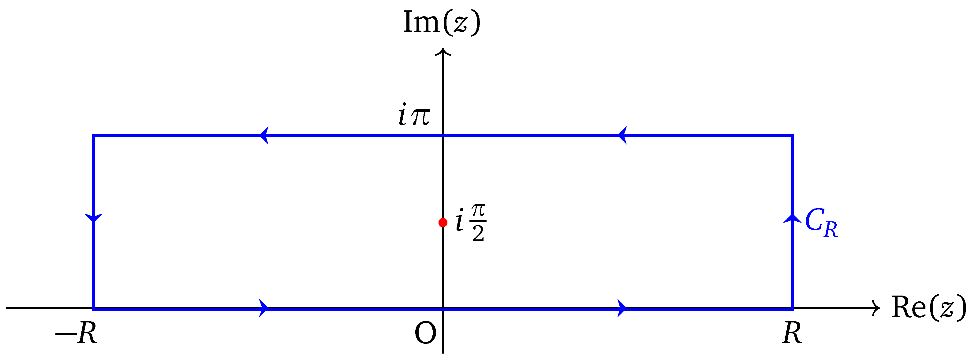
and the rectangular contour $C_R$ in the complex plane with corners at $\pm R$ and $\pm R+i\pi$, with $R>0$, as shown in Figure 1.

The function $\varphi \left(z\right)$ (6) has only one pole inside the region bounded by the rectangular contour $C_R$ at $z=i\frac{\pi }{2}$. Hence, according to the consequence of Cauchy’s residue theorem [44,45,46], we can calculate that the contour integral over $C_R$ is given by

$$\begin{array}{c}\begin{array}{cc}\hfill \underset{C_R}{\int }\varphi \left(z\right)dz& =2\pi i\mathrm{Res}\left(\varphi ,i\frac{\pi }{2}\right)=2\pi i\frac{2cos\left(ki\frac{\pi }{2}\right)}{e^{i\frac{\pi }{2}}-e^{-i\frac{\pi }{2}}}\hfill \\ & =2\pi i\frac{2cosh\left(\frac{\pi }{2}k\right)}{2isin\frac{\pi }{2}}=2\pi cosh\left(\frac{\pi }{2}k\right).\hfill \end{array}\end{array}$$

(7)

Concurrently, this very same contour integral can also be expressed as four separate distinct line integrals along each side of the rectangle. We thus have

$$\begin{array}{cc}\hfill \underset{C_R}{\int }\varphi \left(z\right)dz& ={\int }_{-R}^R\frac{2coskx}{e^x+e^{-x}}dx+{\int }_0^{\pi }\frac{2cosk\left(R+iy\right)}{e^{R+iy}+e^{-R-iy}}idy\hfill \\ \hfill & -{\int }_{-R}^R\frac{2cosk\left(x+\pi i\right)}{e^{x+\pi i}+e^{-x-\pi i}}dx-{\int }_0^{\pi }\frac{2cosk\left(-R+iy\right)}{e^{-R+iy}+e^{R-iy}}idy.\hfill \end{array}$$

(8)

Now, observe that the integrand of the second integral can be expressed as follows for sufficiently large R:

$$\begin{array}{cc}\hfill \left|\frac{2cosk\left(R+iy\right)}{e^{R+iy}+e^{-R-iy}}\right|& =\left|\frac{e^{ikR}{e}^{-ky}+e^{-ikR}{e}^{ky}}{e^{R+iy}+e^{-R-iy}}\right|=\left|\frac{e^{\left(1+ik\right)R}{e}^{\left(-k+i\right)y}+e^{\left(1-ik\right)R}{e}^{\left(k+i\right)y}}{e^{2\left(R+iy\right)}+1}\right|\hfill \\ \hfill & \le \left|\frac{e^{\left(1+ik\right)R}{e}^{\left(-k+i\right)y}}{e^{2\left(R+iy\right)}+1}\right|+\left|\frac{e^{\left(1-ik\right)R}{e}^{\left(k+i\right)y}}{e^{2\left(R+iy\right)}+1}\right|\hfill \\ \hfill & \le \frac{e^{R-ky}}{e^{2R}-1}+\frac{e^{R+ky}}{e^{2R}-1}=\frac{2e^{R}coshky}{e^{2R}-1}\le 4e^{-R}coshky.\hfill \end{array}$$

Thus, the absolute value of the second integral reads

$$\begin{array}{cc}\hfill \left|{\int }_0^{\pi }\frac{2cosk\left(R+iy\right)}{e^{R+iy}+e^{-R-iy}}idy\right|& \le {\int }_0^{\pi }\left|\frac{2cosk\left(R+iy\right)}{e^{R+iy}+e^{-R-iy}}i\right|dy\hfill \\ \hfill & \le {\int }_0^{\pi }4e^{-R}coshkydy=4e^{-R}sinhk\pi ,\hfill \end{array}$$

which tends to 0 as $R\to \infty$. Similarly, for sufficiently large R, the function of the fourth integral satisfies the following relationship:

$$\begin{array}{cc}\hfill \left|\frac{2cosk\left(-R+iy\right)}{e^{-R+iy}+e^{R-iy}}\right|& =\left|\frac{e^{-ikR}{e}^{-ky}+e^{ikR}{e}^{ky}}{e^{-R+iy}+e^{R-iy}}\right|=\left|\frac{e^{-\left(1+ik\right)R}{e}^{\left(-k+i\right)y}+e^{\left(-1+ik\right)R}{e}^{\left(k+i\right)y}}{1+e^{-2\left(R-iy\right)}}\right|\hfill \\ \hfill & \le \frac{\left|e^{-\left(1+ik\right)R}{e}^{\left(-k+i\right)y}\right|+\left|e^{\left(-1+ik\right)R}{e}^{\left(k+i\right)y}\right|}{\left|1+e^{-2\left(R-iy\right)}\right|}\hfill \\ \hfill & \le \frac{e^{-R-ky}+e^{-R+ky}}{1-e^{-2R}}=\frac{2e^{-R}coshky}{1-e^{-2R}}\le 2e^{-R}coshky.\hfill \end{array}$$

Therefore, the absolute value of the fourth integral becomes

$$\begin{array}{cc}\hfill \left|{\int }_0^{\pi }\frac{2cosk\left(-R+iy\right)}{e^{-R+iy}+e^{R-iy}}idy\right|& \le {\int }_0^{\pi }\left|\frac{2cosk\left(-R+iy\right)}{e^{-R+iy}+e^{R-iy}}i\right|dy\hfill \\ \hfill & \le {\int }_0^{\pi }2e^{-R}coshkydy=2e^{-R}sinhk\pi ,\hfill \end{array}$$

which again tends to 0 as $R\to \infty$. Considering the third integral, it follows that

$$\begin{array}{cc}\hfill -{\int }_{-R}^R\frac{2cosk\left(x+\pi i\right)}{e^{x+\pi i}+e^{-x-\pi i}}dx& ={\int }_{-R}^R\frac{e^{ikx}{e}^{-\pi k}+e^{-ikx}{e}^{\pi k}}{e^x+e^{-x}}dx\hfill \\ \hfill & ={\int }_{-R}^R\frac{coskxcosh\pi k}{coshx}dx-i{\int }_{-R}^R\frac{sinkxsinh\pi k}{coshx}dx\hfill \\ \hfill & =cosh\pi k{\int }_{-R}^R\frac{coskx}{coshx}dx,\hfill \end{array}$$

where the imaginary component of the integral vanishes since $sin\left(kx\right)$ is an odd function. Hence, letting $R\to \infty$, we observe from (7) and (8) that

$$\underset{R\to \infty }{lim}\left(1+cosh\pi k\right){\int }_{-R}^R\frac{coskx}{coshx}dx=\left(1+cosh\pi k\right){\int }_{-\infty }^{\infty }\frac{coskx}{coshx}dx=2\pi cosh\left(\frac{\pi }{2}k\right).$$

Therefore,

$$\begin{array}{cc}\hfill {\int }_{-\infty }^{\infty }\frac{coskx}{coshx}dx& =\frac{2\pi cosh\left(\frac{\pi }{2}k\right)}{1+cosh\pi k}=\frac{2\pi cosh\left(\frac{\pi }{2}k\right)}{2{cosh}^2\left(\frac{\pi }{2}k\right)}=\frac{\pi }{cosh\left(\frac{\pi }{2}k\right)}=\pi \mathrm{sech}\left(\frac{\pi }{2}k\right),\hfill \end{array}$$

and thus, the spatial Fourier transform for the bright soliton is given by

$$\widehat{q}(k,t)=\pi \mathrm{sech}\left(\frac{\pi }{2}k\right)e^{it}.$$

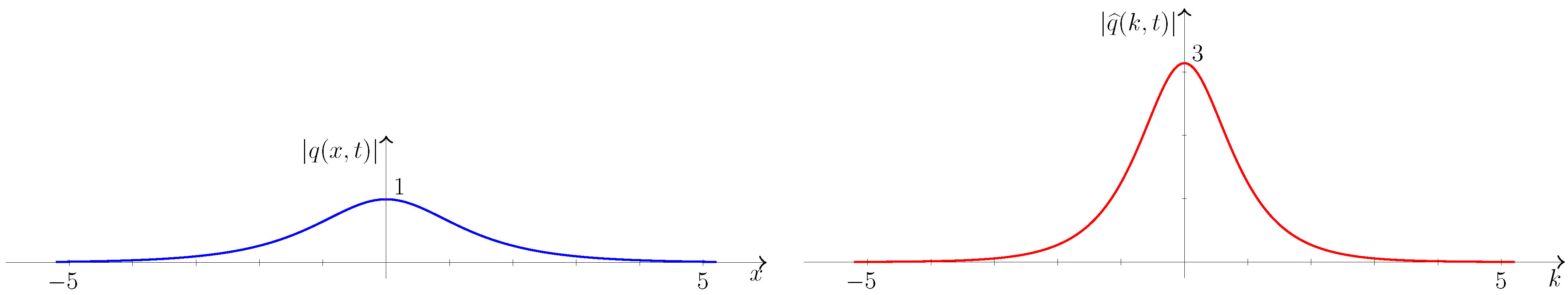
This completes the proof and Figure 2 displays the moduli of the bright soliton and its corresponding Fourier spectrum. □

2.2. Fourier Spectrum as Infinite Series

A similar approach in calculating the bright soliton spectrum yields an expression of convergent alternating series form, where the integral of the associated Fourier transform is expressed as Gauss’s hypergeometric function [47]:

$$\widehat{q}(k,t)=4e^{it}\sum _{n=0}^{\infty }{(-1)}^n\frac{2n+1}{k^2+{\left(2n+1\right)}^2}.$$

We need the following lemma and the summation theorem to prove the above result [44,48,49,50].

Theorem 2 

(Mittag–Leffler’s expansion theorem). Let $p\left(z\right)$ be a complex-valued function with singularities in the finite complex plane that are only the simple poles ${\zeta }_1$, ${\zeta }_2$, ${\zeta }_3$, ⋯, which are arranged in the order of increasing modulus, with Res $\left(p\left(z\right);{\zeta }_n\right)={\mu }_n$, $n\in \mathbb{N}$. Let also $C_N$ be circles of radius $R_N$ that do not pass through any poles and for which $\left|p\left(z\right)\right|<M$, where M is independent of N and $R_N\to \infty$ as $N\to \infty$. Then, Mittag–Leffler’s expansion theorem states that

$$p\left(z\right)=p\left(0\right)+\sum _{n=1}^{\infty }{\mu }_n\left(\frac{1}{z-{\zeta }_n}+\frac{1}{{\zeta }_n}\right).$$

The readers who are interested to see the proof of this theorem may consult [48].

Lemma 1. 

The function $\mathrm{sech}\left(\frac{\pi }{2}z\right)$ is bounded on the circles $C_N$ having the center at the origin and radius $R_N=\left(2N+\frac{3}{4}\right)$, $N\in {\mathbb{N}}_0$.

Proof. 

Since $z=x+iy$ as usual, then the real and imaginary parts satisfy the equation of the circle $x^2+y^2=R_N^2$. Consider the reciprocal of this hyperbolic secant function, i.e., $cosh\left(\frac{\pi }{2}z\right)$. We attempt to find its lower bound for any value of z inside of or at the circles $C_N$. We know the following hyperbolic function identity:

$${\left|cosh\left(\frac{\pi }{2}z\right)\right|}^2={sinh}^2\left(\frac{\pi }{2}x\right)+{cos}^2\left(\frac{\pi }{2}y\right)\ge \frac{{\pi }^2}{4}{x}^2+{cos}^2\left(\frac{\pi }{2}y\right).$$

(9)

Obviously, $0\le {cos}^2\left(\frac{\pi }{2}y\right)\le 1$ for all $y\in \mathbb{R}$, but we will consider two different cases, i.e., $\frac{1}{2}\le {cos}^2\left(\frac{\pi }{2}y\right)\le 1$ when $\left|y-2N\right|\le \frac{1}{2}$ and $0\le {cos}^2\left(\frac{\pi }{2}y\right)\le \frac{1}{2}$ when $\left|y-2N\right|\ge \frac{1}{2}$, $N\in \mathbb{Z}$. From the former, we obtain $y\le 2N+\frac{1}{2}$, $y^2\le {\left(2N+\frac{1}{2}\right)}^2$ and $-y^2\ge -{\left(2N+\frac{1}{2}\right)}^2$. Upon substitution of the inequality (9), we obtain

$$\begin{array}{cc}\hfill {\left|cosh\left(\frac{\pi }{2}z\right)\right|}^2& \ge \frac{{\pi }^2}{4}\left(R^2-y^2\right)+\frac{1}{2}\hfill \\ \hfill & \ge \frac{{\pi }^2}{4}\left[{\left(2N+\frac{3}{4}\right)}^2-{\left(2N+\frac{1}{2}\right)}^2\right]+\frac{1}{2}\ge \frac{5{\pi }^2}{64}+\frac{1}{2},\hfill \\ \hfill \mathrm{or}\left|cosh\left(\frac{\pi }{2}z\right)\right|& \ge \frac{\sqrt{5{\pi }^2+32}}{8}.\hfill \end{array}$$

Thus, we have an upper bound for $\mathrm{sech}\left(\frac{\pi }{2}z\right)$ when $\left|y-2N\right|\le \frac{1}{2}$, $N\in \mathbb{Z}$:

$$\left|\mathrm{sech}\left(\frac{\pi }{2}z\right)\right|\le \frac{8}{\sqrt{32+5{\pi }^2}}.$$

For the second case, we obtain either $y\ge 2N+\frac{1}{2}$ or $y\le 2N-\frac{1}{2}$. By focusing on the latter, we acquire $-y^2\ge -{\left(2N-\frac{1}{2}\right)}^2$. Employing again the inequality (9), but now dropping the term ${cos}^2\left(\frac{\pi }{2}y\right)$ because it is always non-negative, we arrive at

$$\begin{array}{cc}\hfill {\left|cosh\left(\frac{\pi }{2}z\right)\right|}^2& \ge \frac{{\pi }^2}{4}\left(R^2-y^2\right)\ge \frac{{\pi }^2}{4}\left[{\left(2N+\frac{3}{4}\right)}^2-{\left(2N-\frac{1}{2}\right)}^2\right]+\frac{1}{2}\ge \frac{5{\pi }^2}{64}.\hfill \end{array}$$

An upper bound for $\mathrm{sech}\left(\frac{\pi }{2}z\right)$ when $\left|y-2N\right|\ge \frac{1}{2}$ is therefore:

$$\left|\mathrm{sech}\left(\frac{\pi }{2}z\right)\right|\le \frac{8}{\pi \sqrt{5}}.$$

Taking the largest between the two upper bounds, we take the latter, and this completes the proof. □

Note that a sharper upper bound can be obtained if we take additional terms in the Taylor series expansion for the hyperbolic sine function, e.g., instead of using ${sinh}^2\left(\frac{\pi }{2}x\right)\ge \frac{{\pi }^2}{4}{x}^2$, we could take

$${sinh}^2\left(\frac{\pi }{2}x\right)\ge \frac{{\pi }^2}{4}{x}^2\left(1+\frac{{\pi }^2}{12}{x}^2\right)$$

instead. For the sake of simplicity, considering only one term suffices, as demonstrated in the proof above. We are now ready to state and prove the following important proposition.

Proposition 1. 

For $k\in \mathbb{R}$, the hyperbolic secant function can be expressed as an alternating infinite series:

$$\mathrm{sech}\left(\frac{\pi }{2}k\right)=\frac{4}{\pi }\sum _{n=0}^{\infty }\frac{{(-1)}^n\left(2n+1\right)}{k^2+{(2n+1)}^2}.$$

Proof. 

Consider the complex-valued function:

$$p\left(z\right)=\mathrm{sech}\left(\frac{\pi }{2}z\right)=\frac{1}{cosh\left(\frac{\pi }{2}z\right)},$$

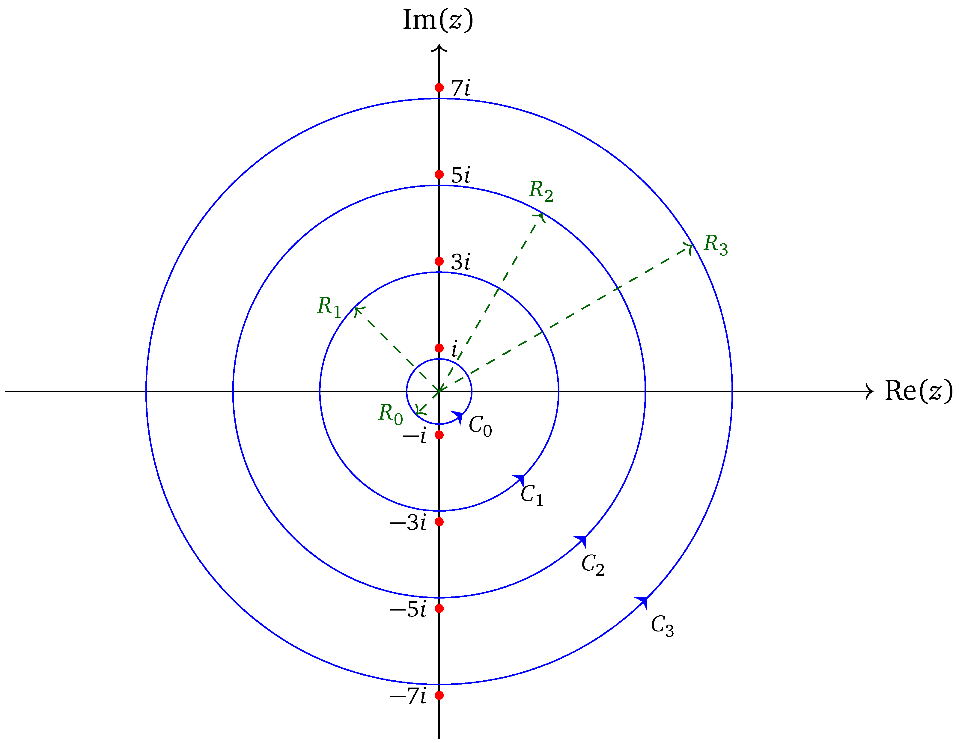
then $p\left(0\right)=1$ and $p\left(z\right)$ has simple poles at ${\zeta }_n=\left(2n+1\right)i$, $n\in \mathbb{Z}$. See Figure 3. Using the fact that $\mathrm{csch}\left(iz\right)=-icsc\left(z\right)$ and $csc\left(z+\frac{\pi }{2}\right)=sec\left(z\right)$, we can calculate the residue of $p\left(z\right)$ at these poles:

$$\begin{array}{cc}\hfill \mathrm{Res}\left(p\left(z\right),{\zeta }_n\right)& =\underset{z\to {\zeta }_n}{lim}\left(z-{\zeta }_n\right)\mathrm{sech}\left(\frac{\pi }{2}z\right)=\underset{z\to {\zeta }_n}{lim}\frac{2}{\pi }\mathrm{csch}\left(\frac{\pi }{2}z\right)=\frac{2}{\pi }\mathrm{csch}\left[\frac{\pi }{2}\left(2n+1\right)i\right]\hfill \\ \hfill & =-\frac{2i}{\pi }csc\left(\pi n-\frac{\pi }{2}\right)=-\frac{2i}{\pi }sec\left(\pi n\right)=\frac{2i}{\pi }{\left(-1\right)}^{n+1}.\hfill \end{array}$$

Furthermore, as shown in Lemma 1, $p\left(z\right)$ is bounded on circles $C_N$ that are centered at the origin with radius $R_N=\left(2N+\frac{3}{4}\right)$, as depicted in Figure 3. Using the well-known Leibniz–Gregory–Nilakantha formula for $\pi$ [51,52,53]:

$$\frac{\pi }{4}=\sum _{n=0}^{\infty }\frac{{(-1)}^n}{2n+1}=1-\frac{1}{3}+\frac{1}{5}-\frac{1}{7}+\frac{1}{9}-\cdots ,$$

(10)

we obtain

$$\begin{array}{cc}\hfill \mathrm{sech}\left(\frac{\pi }{2}z\right)& =1+\sum _{n=-\infty }^{\infty }\frac{2i}{\pi }{\left(-1\right)}^{n+1}\left(\frac{1}{z-\left(2n+1\right)i}+\frac{1}{\left(2n+1\right)i}\right)\hfill \\ \hfill & =1+\frac{2}{\pi }\sum _{n=-\infty }^{\infty }{\left(-1\right)}^n\left(\frac{1}{iz+\left(2n+1\right)}-\frac{1}{2n+1}\right)\hfill \\ \hfill & =\frac{2}{\pi }\left[\left(\frac{1}{iz+1}-\frac{1}{iz-1}\right)-\left(\frac{1}{iz+3}-\frac{1}{iz-3}\right)+\left(\frac{1}{iz+5}-\frac{1}{iz-5}\right)-\cdots \right]\hfill \\ \hfill & +1-\frac{4}{\pi }\left(1-\frac{1}{3}+\frac{1}{5}-\cdots \right)\hfill \\ \hfill & =\frac{4}{\pi }\left(\frac{1}{z^2+1^2}-\frac{3}{z^2+3^2}+\frac{5}{z^2+5^2}-\cdots \right)=\frac{4}{\pi }\sum _{n=0}^{\infty }\frac{{(-1)}^n\left(2n+1\right)}{z^2+{(2n+1)}^2}.\hfill \end{array}$$

Taking real-valued $z=k\in \mathbb{R}$, we obtain the desired equality, and the proof is complete. □

To verify the converse of the statement, we use the following lemma and summation theorem.

Lemma 2. 

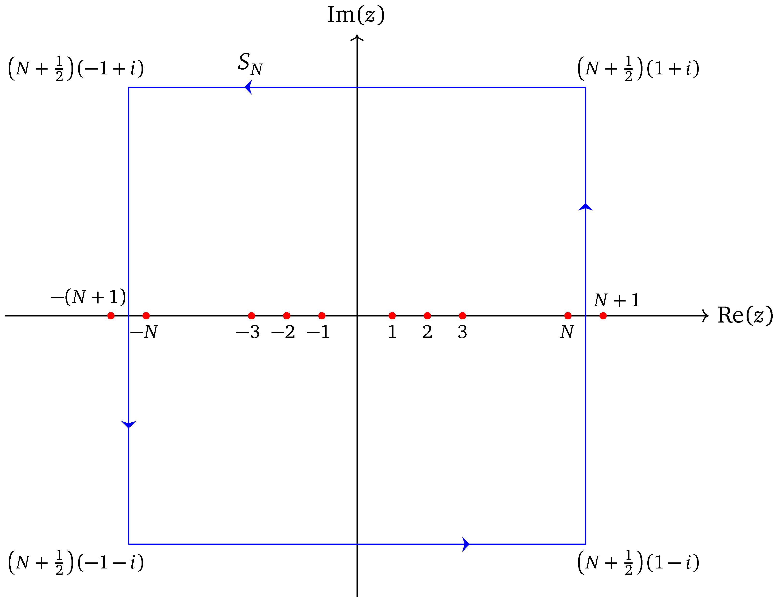
Let $N\in \mathbb{N}$, and let $S_N$ be the square with corners at $\left(N+\frac{1}{2}\right)\left(\pm 1\pm i\right)$ as illustrated in Figure 4, then there exist positive constants A and B such that $\left|cot\left(\pi z\right)\right|\le A$ and $\left|csc\left(\pi z\right)\right|\le B$ for all z in the square $S_N$.

Proof. 

On the horizontal sides of the square, we have $z=x\pm i\left(N+\frac{1}{2}\right)$. Because

$$\begin{array}{cc}\hfill \left|e^{i\pi x}{e}^{\mp \pi \left(N+\frac{1}{2}\right)}+e^{-i\pi x}{e}^{\pm \pi \left(N+\frac{1}{2}\right)}\right|& \le \left|e^{i\pi x}\right|e^{\mp \pi \left(N+\frac{1}{2}\right)}+\left|e^{-i\pi x}\right|e^{\pm \pi \left(N+\frac{1}{2}\right)}\hfill \\ \hfill & =e^{\pi \left(N+\frac{1}{2}\right)}+e^{-\pi \left(N+\frac{1}{2}\right)},\hfill \\ \hfill \left|e^{i\pi x}{e}^{\mp \pi \left(N+\frac{1}{2}\right)}-e^{-i\pi x}{e}^{\pm \pi \left(N+\frac{1}{2}\right)}\right|& \ge e^{\pi \left(N+\frac{1}{2}\right)}-e^{-\pi \left(N+\frac{1}{2}\right)},\hfill \end{array}$$

and the hyperbolic cotangent function is decreasing in the interval $\left(0,\infty \right)$, we deduce that

$$\begin{array}{cc}\hfill \left|cot\left(\pi z\right)\right|& =\left|\frac{cos\left(\pi z\right)}{sin\left(\pi z\right)}\right|=\left|\frac{e^{i\pi z}+e^{-i\pi z}}{e^{i\pi z}-e^{-i\pi z}}\right|=\left|\frac{e^{i\pi \left[x\pm i\left(N+\frac{1}{2}\right)\right]}+e^{-i\pi \left[x\pm i\left(N+\frac{1}{2}\right)\right]}}{e^{i\pi \left[x\pm i\left(N+\frac{1}{2}\right)\right]}-e^{-i\pi \left[x\pm i\left(N+\frac{1}{2}\right)\right]}}\right|\hfill \\ \hfill & \le \frac{e^{\pi \left(N+\frac{1}{2}\right)}+e^{-\pi \left(N+\frac{1}{2}\right)}}{e^{\pi \left(N+\frac{1}{2}\right)}-e^{-\pi \left(N+\frac{1}{2}\right)}}=\frac{cosh\left(N+\frac{1}{2}\right)\pi }{sinh\left(N+\frac{1}{2}\right)\pi }=coth\left(N+\frac{1}{2}\right)\pi \le coth\frac{3}{2}\pi .\hfill \end{array}$$

On the vertical sides, we have $z=\pm \left(N+\frac{1}{2}\right)+iy$. Employing the trigonometric identities $cot\left(N\pm \frac{\pi }{2}\right)=-tanz$ and $cot\left(z\pm N\pi \right)=cotz$, we obtain

$$\left|cot\left(\pi z\right)\right|=\left|cot\left(\pm N\pi \pm \frac{\pi }{2}+i\pi y\right)\right|=\left|-itan\left(i\pi y\right)\right|=\left|tanh\left(\pi y\right)\right|\le 1,$$

since ${tanh}^2\left(\pi y\right)=1-\mathrm{sech}{}^2\left(\pi y\right)$ for all $y\in \mathbb{R}$.

Using a similar argument, on the horizontal sides, the cosecant function can be expressed as follows:

$$\begin{array}{cc}\hfill \left|csc\left(\pi z\right)\right|& =\left|\frac{1}{sin\left(\pi z\right)}\right|=\left|\frac{2i}{e^{i\pi z}-e^{-i\pi z}}\right|=\left|\frac{2}{e^{i\pi \left[x\pm i\left(N+\frac{1}{2}\right)\right]}-e^{-i\pi \left[x\pm i\left(N+\frac{1}{2}\right)\right]}}\right|\hfill \\ \hfill & \le \frac{2}{e^{\pi \left(N+\frac{1}{2}\right)}-e^{-\pi \left(N+\frac{1}{2}\right)}}=\mathrm{csch}\left(N+\frac{1}{2}\right)\pi \le \mathrm{csch}\left(\frac{3}{2}\pi \right),\hfill \end{array}$$

because the hyperbolic cosecant function is decreasing in the interval $\left(0,\infty \right)$. On the vertical sides of the rectangle, we utilize the identities $csc\left(z\pm \frac{\pi }{2}\right)=\pm secz$ and $csc\left(z\pm N\pi \right)={\left(-1\right)}^{N}cscz$ to show that

$$\left|csc\left(\pi z\right)\right|=\left|csc\left(\pm N\pi \pm \frac{\pi }{2}+i\pi y\right)\right|=\left|sec\left(i\pi y\right)\right|=\left|\mathrm{sech}\left(\pi y\right)\right|\le 1,$$

because $\mathrm{sech}{}^2\left(\pi y\right)=1-{tanh}^2\left(\pi y\right)$ for all $y\in \mathbb{R}$. Hence, we can take $A=coth\frac{3}{2}\pi \ge 1$ and $B=1\ge \mathrm{csch}\left(\frac{3}{2}\pi \right)$, and the proof is complete. □

Note that the constant 2 in the numerator for the cosecant and the factor $\pi$ in the argument for the secant and hyperbolic secant functions were missing in [44], and they have been restored here. The constants A and B are certainly not unique, and different values of these constants are possible, as demonstrated in [48], where the authors proved this by splitting the portions of the square $S_n$ into several regions depending on the imaginary variable y, i.e., $y<-\frac{1}{2}$, $\left|y\right|<\frac{1}{2}$, and $y>\frac{1}{2}$.

Theorem 3 

(Summation theorem). Let $f\left(z\right)$ be a function that is differentiable on $\mathbb{C}$ except for finitely many poles $z_1$, $z_2,\cdots$, $z_r$, none of which is a real-valued integer. Suppose also that there exist positive constants K and R such that $\left|z^{2}f\left(z\right)\right|\le K$ whenever $\left|z\right|>R$. Let

$$g\left(z\right)=\pi f\left(z\right)cot\left(\pi z\right)\mathit{and}h\left(z\right)=\pi f\left(z\right)csc\left(\pi z\right),$$

then

$$\begin{array}{c}\begin{array}{cc}\hfill \sum _{n=-\infty }^{\infty }f\left(n\right)& =-\sum _{j=1}^r\mathit{Res}\left(g\left(z\right),z_j\right)\mathit{and}\hfill \\ \hfill \sum _{n=-\infty }^{\infty }{(-1)}^{n}f\left(n\right)& =-\sum _{j=1}^r\mathit{Res}\left(h\left(z\right),z_j\right).\hfill \end{array}\end{array}$$

(11)

Note that the assumption of $1/f\left(z\right)$ is a polynomial function with real coefficients, degree $n\ge 2$, and no integer zeros, as stated in [50], belonging to only some special cases of $f\left(z\right)$.

Proof. 

Since $\left|f\left(n\right)\right|\le \frac{K}{n^2}$ whenever $\left|n\right|>R$ for $n\in \mathbb{Z}$, then both series $\sum f\left(n\right)$ and $\sum {\left(-1\right)}^{n}f\left(n\right)$ are absolutely convergent, and thus, they are convergent. Furthermore, for both functions $\pi cot\left(\pi z\right)$ and $\pi csc\left(\pi z\right)$, the set of poles is the set of real-valued integers $n\in \mathbb{Z}$. Consequently, the set of poles for both functions g and h is $\left\{z_1,z_2,\cdots ,z_r\right\}\cup \mathbb{Z}$. By the periodic properties of the circular functions, we can express $cot\left(\pi z\right)=cot\pi \left(z-n\right)$ and $csc\left(\pi z\right)={\left(-1\right)}^{n}csc\pi \left(z-n\right)$. Therefore, the residues of these functions are given by

$$\begin{array}{cc}\hfill \mathrm{Res}\left(cot\left(\pi z\right),n\right)& =\underset{z\to n}{lim}\left(z-n\right)cot\left(\pi z\right)=\underset{z\to n}{lim}\left(z-n\right)cot\pi \left(z-n\right)\hfill \\ \hfill & =\underset{z\to n}{lim}cos\pi \left(z-n\right)\frac{z-n}{sin\pi \left(z-n\right)}=\frac{1}{\pi },\hfill \\ \hfill \mathrm{Res}\left(csc\left(\pi z\right),n\right)& =\underset{z\to n}{lim}\left(z-n\right)csc\left(\pi z\right)=\underset{z\to n}{lim}{\left(-1\right)}^n\frac{z-n}{sin\pi \left(z-n\right)}=\frac{{(-1)}^n}{\pi }.\hfill \end{array}$$

Furthermore, when the function f generally possesses no zeros on the (real) x-axis, but each of both functions g and h has a simple pole at each integer n, we can calculate their residues at $z=n\in \mathbb{Z}$:

$$\begin{array}{cc}\hfill \mathrm{Res}\left(g\left(z\right),n\right)& =\underset{z\to n}{lim}\pi f\left(z\right)\left(z-n\right)cot\left(\pi z\right)=f\left(n\right),\mathrm{and}\hfill \\ \hfill \mathrm{Res}\left(h\left(z\right),n\right)& =\underset{z\to n}{lim}\pi f\left(z\right)\left(z-n\right)csc\left(\pi z\right)={\left(-1\right)}^{n}f\left(n\right).\hfill \end{array}$$

Meanwhile, from Cauchy’s residue theorem, we have

$$\begin{array}{cc}\hfill \underset{S_N}{\int }g\left(z\right)dz& =2\pi i\left(\sum _{n=-R}^R\mathrm{Res}\left(g\left(z\right),n\right)+\sum _{j=1}^r\mathrm{Res}\left(g\left(z\right),z_j\right)\right),\mathrm{and}\hfill \\ \hfill \underset{S_N}{\int }h\left(z\right)dz& =2\pi i\left(\sum _{n=-R}^R\mathrm{Res}\left(h\left(z\right),n\right)+\sum _{j=1}^r\mathrm{Res}\left(h\left(z\right),z_j\right)\right).\hfill \end{array}$$

Since the contour of $S_N$ has a total length of $4(2N+1)$, using Lemma 2 and for sufficiently large N, we obtain

$$\begin{array}{cc}\hfill \left|\underset{S_N}{\int }g\left(z\right)dz\right|& \le \underset{S_N}{\int }\left|\pi f\left(z\right)cot\left(\pi z\right)dz\right|\le 4\left(2N+1\right)\underset{z\in S_N}{sup}\left|\pi f\left(z\right)cot\left(\pi z\right)\right|\hfill \\ \hfill & \le 4\left(2N+1\right)\frac{KA}{N^2},\mathrm{and}\hfill \\ \hfill \left|\underset{S_N}{\int }h\left(z\right)dz\right|& \le \underset{S_N}{\int }\left|\pi f\left(z\right)csc\left(\pi z\right)dz\right|\le 4\left(2N+1\right)\underset{z\in S_N}{sup}\left|\pi f\left(z\right)csc\left(\pi z\right)\right|\hfill \\ \hfill & \le 4\left(2N+1\right)\frac{KB}{N^2}.\hfill \end{array}$$

Both of these upper bounds tend to 0 as $N\to \infty$. Hence, by letting $N\to \infty$ (or $R\to \infty$), we obtain

$$\begin{array}{cc}\hfill \sum _{n=-\infty }^{\infty }f\left(n\right)+\sum _{j=1}^r\mathrm{Res}\left(g\left(z\right),z_j\right)& =0,\mathrm{and}\hfill \\ \hfill \sum _{n=-\infty }^{\infty }{\left(-1\right)}^{n}f\left(n\right)+\sum _{j=1}^r\mathrm{Res}\left(h\left(z\right),z_j\right)& =0,\hfill \end{array}$$

for which the equalities in (11) are established and the proof is complete. □

We state and prove another important proposition, which is the converse of Proposition 1, by leading an infinite series into a closed analytical form.

Proposition 2. 

For any $k\in \mathbb{R}$, the following alternating series converges, and it can be simplified into a hyperbolic secant function in k:

$$\sum _{n=0}^{\infty }\frac{{\left(-1\right)}^n\left(2n+1\right)}{k^2+{\left(2n+1\right)}^2}=\frac{\pi }{4}\mathrm{sech}\left(\frac{\pi }{2}k\right).$$

(12)

Proof. 

To prove the convergence, we apply the alternating series test. Let

$$a_n\left(k\right)={\left(-1\right)}^n{b}_n\left(k\right),\mathrm{where}{b}_n\left(k\right)=\frac{\left(2n+1\right)}{k^2+{\left(2n+1\right)}^2},n\in {\mathbb{N}}_0,k\in \mathbb{R},$$

then

$$\begin{array}{cc}\hfill b_{n+1}\left(k\right)& =\frac{\left(2n+3\right)}{k^2+{\left(2n+3\right)}^2}\le \frac{\left(2n+1\right)}{k^2+{\left(2n+1\right)}^2}=b_n\left(k\right),\hfill \\ \hfill \underset{n\to \infty }{lim}{b}_n\left(k\right)& =\underset{n\to \infty }{lim}\frac{\left(2n+1\right)}{k^2+{\left(2n+1\right)}^2}=0.\hfill \end{array}$$

Since the absolute value of the terms is getting smaller and tends to zero as n goes to infinity, the alternating series is thus convergent. To find a particular function where it converges, let

$$f\left(z\right)=\frac{2z+1}{k^2+{\left(2z+1\right)}^2},k\in \mathbb{R},$$

then f possesses two poles $z_1$ and $z_2$:

$$z_{1,2}=-\frac{1}{2}\left(1\mp ik\right).$$

By expressing the left-hand side of (12) as the summation over $n\in \mathbb{Z}$ and applying Theorem 3, we demonstrate that it arrives at the expression on the right-hand side of (12):

$$\begin{array}{cc}\hfill \sum _{n=0}^{\infty }\frac{{(-1)}^n(2n+1)}{k^2+{(2n+1)}^2}& =\frac{1}{2}\sum _{n=-\infty }^{\infty }\frac{{(-1)}^n(2n+1)}{k^2+{(2n+1)}^2}=-\frac{1}{2}\sum _{j=1}^2\mathrm{Res}\left(\frac{\pi (2z+1)csc\left(\pi z\right)}{k^2+{(2z+1)}^2};z_j\right)\hfill \\ \hfill & =-\frac{1}{2}\left\{\frac{\pi }{4}csc\frac{\pi }{2}\left(ik-1\right)+\frac{\pi }{4}csc\left[-\frac{\pi }{2}\left(ik+1\right)\right]\right\}\hfill \\ \hfill & =\frac{\pi }{8}\left[sec\left(\frac{\pi }{2}ik\right)+sec\left(-\frac{\pi }{2}ik\right)\right]=\frac{\pi }{8}\left[\mathrm{sech}\left(\frac{\pi }{2}k\right)+\mathrm{sech}\left(\frac{\pi }{2}k\right)\right]\hfill \\ \hfill & =\frac{\pi }{4}\mathrm{sech}\left(\frac{\pi }{2}k\right).\hfill \end{array}$$

This completes the proof. □

For $k=0$, we recover the Leibniz–Gregory–Nilakantha formula for $\pi$ (10) [51,52,53].

3. Soliton Characteristics

This section examines some characteristics of the fundamental bright soliton and its corresponding spatial Fourier spectrum. Understanding the properties and characteristics of this soliton—or any other waves—in the spatial and Fourier domains is particularly essential from the viewpoint of the applications. Some soliton’s features that are not obviously captured in one domain during its evolution might be distinctly visible in the other domain, and vice versa. In water waves, for example, the asymmetric pattern of the wave signal is closely correlated to the frequency downshift in the spectral domain [47,54]. In digital communications, any changes in the spectral width may have a direct bearing on the communication system’s capacity and on the equipment design, which accommodates certain wave characteristics [55]. As we will observe in this section, the width of the soliton in both domains is inversely related. A contraction in one domain yields an expansion in the other domain.

Although the literature usually considers the temporal–frequency domain relationship, i.e., pulse or signal (together with its envelope) in the time domain and its temporal Fourier spectrum in the frequency domain, we focus on the relationship of the spatial-wavenumber domains. Hence, some terminologies in the definition are adjusted to the related domains accordingly. We commence with the following definitions and propositions.

Definition 3 

(Soliton power and energy spectral density). The squared-absolute value of the fundamental bright soliton ${\left|q(x,t)\right|}^2$ is called the (envelope) soliton power, whereas the associated squared-modulus of its spatial Fourier spectrum ${\left|\widehat{q}(k,t)\right|}^2$ is called the energy spectral density [56].

Figure 2 displays the envelope power of the bright soliton (left panel) and its associated energy spectral density (right panel) for a fixed value of $t\in \mathbb{R}$. We observe that the Fourier transform preserves the hyperbolic secant profile, albeit with different heights and widths between the spatial and wavenumber domains.

Definition 4 

(Soliton energy). The integral of the soliton power is called the soliton energy, and it satisfies Parseval’s theorem in the spatial-wavenumber domains [57]:

$$E={\int }_{-\infty }^{\infty }{\left|q\left(x,t\right)\right|}^{2}dx=\frac{1}{2\pi }{\int }_{-\infty }^{\infty }{\left|\widehat{q}\left(k,t\right)\right|}^{2}dk.$$

(13)

This soliton energy is also called the number of quanta, with the integral on the left-hand side of (13) being identical to the first integral of motion, a conserved quantity in the NLS integrable system [36]. Higher-order conserved quantities exist, and in particular, the second and third integrals of motion correspond to the momentum and Hamiltonian, respectively [23,58,59,60,61].

The definition of the integral of the energy spectral density seems to be absent in the literature since it equals the soliton energy, which can be calculated through either $q(x,t)$ or $\widehat{q}(k,t)$. Indeed, the relationship between these two quantities is encapsulated by a fundamental property of Fourier transforms known as Parseval’s theorem (13), which states that the soliton energy equals the area under the square of the magnitude of the Fourier transform of the soliton profile divided by $2\pi$. If one wishes to define the latter, the total energy spectrum is not a bad option.

Proposition 3. 

The fundamental bright soliton satisfies Parseval’s theorem (13) in the spatial-wavenumber domains [62].

Proof. 

On the one hand, the expression for the soliton energy (13) is given by

$$\begin{array}{cc}\hfill {\int }_{-\infty }^{\infty }{\left|q\left(x,t\right)\right|}^{2}dx& ={\int }_{-\infty }^{\infty }\mathrm{sech}{}^{2}xdx=\underset{c\to \infty }{lim}{\int }_{-c}^c\mathrm{sech}{}^{2}xdx=\underset{c\to \infty }{lim}tanhx{|}_{-c}^c\hfill \\ \hfill & =\underset{c\to \infty }{lim}\left[tanhc-tanh\left(-c\right)\right]=\left[1-\left(-1\right)\right]=2.\hfill \end{array}$$

On the other hand, the right-hand side of (13) calculates

$$\begin{array}{cc}\hfill \frac{1}{2\pi }{\int }_{-\infty }^{\infty }{\left|\widehat{q}(k,t)\right|}^{2}dk& =\frac{1}{2\pi }{\int }_{-\infty }^{\infty }{\pi }^2\mathrm{sech}{}^2\left(\frac{\pi }{2}k\right)dk=\frac{\pi }{2}\underset{d\to \infty }{lim}{\int }_{-d}^d\mathrm{sech}{}^2\left(\frac{\pi }{2}k\right)dk\hfill \\ \hfill & =\underset{d\to \infty }{lim}tanh\left(\frac{\pi }{2}k\right){|}_{-d}^d=\underset{d\to \infty }{lim}\left[tanh\left(\frac{\pi }{2}d\right)-tanh\left(-\frac{\pi }{2}d\right)\right]\hfill \\ \hfill & =\left[1-\left(-1\right)\right]=2.\hfill \end{array}$$

Since we verify that both sides equal two, we complete the proof. □

3.1. Root-Mean-Squared Width

Definition 5 

(Mean/centroid). Let $q(x,t)$ and $\widehat{q}(k,t)$ be a complex-valued soliton amplitude and its associated spatial Fourier spectrum, respectively. Then, the soliton mean or centroid is defined by

$$\overline{x}=\frac{{\displaystyle {\int }_{-\infty }^{\infty }x{\left|q\left(x,t\right)\right|}^{2}dx}}{{\displaystyle {\int }_{-\infty }^{\infty }{\left|q\left(x,t\right)\right|}^{2}dx}}=\frac{1}{E}{\int }_{-\infty }^{\infty }x{\left|q\left(x,t\right)\right|}^{2}dx,$$

whereas the (spatial) spectrum centroid or mean is defined as follows:

$$\overline{k}=\frac{{\displaystyle {\int }_{-\infty }^{\infty }k{\left|\widehat{q}\left(k,t\right)\right|}^{2}dk}}{{\displaystyle {\int }_{-\infty }^{\infty }{\left|\widehat{q}\left(k,t\right)\right|}^{2}dk}}=\frac{1}{2\pi E}{\int }_{-\infty }^{\infty }k{\left|\widehat{q}\left(k,t\right)\right|}^{2}dk,$$

where E is the soliton energy given by (13). We can consider $\overline{x}$ and $\overline{k}$ as the centers of gravity of the energy distribution in the spatial and wavenumber domains, respectively.

Definition 6 

(Power-root-mean-squared soliton width and spectral bandwidth). Let $q(x,t)$ and $\widehat{q}(k,t)$ be a complex-valued soliton amplitude and its associated spatial Fourier spectrum, respectively. The power-root-mean-squared soliton width ${\sigma }_x\ge 0$, also called the soliton standard deviation or soliton radius of gyration is defined as follows:

$${\sigma }_x^2=\frac{1}{E}{\int }_{-\infty }^{\infty }{(x-\overline{x})}^2{\left|q\left(x,t\right)\right|}^{2}dx,$$

whereas the (spatial) power-root-mean-squared spectral bandwidth ${\sigma }_k\ge 0$ is defined by

$${\sigma }_k^2=\frac{1}{2\pi E}{\int }_{-\infty }^{\infty }{\left(k-\overline{k}\right)}^2{\left|\widehat{q}\left(k,t\right)\right|}^{2}dk.$$

In both instances, $\overline{x}$ and $\overline{k}$ denote the soliton and spectrum centroids mentioned earlier in Definition 5, respectively. We can think of ${\sigma }_x$ and ${\sigma }_k$ as the soliton and its associated Fourier spectrum “spreads” in their respective domains, respectively.

Proposition 4. 

The product of the power-root-mean-squared soliton width with its associated spectral bandwidth satisfies the (spatial) stretch-bandwidth reciprocity relationship, also called the space-wavenumber uncertainty relationship [56,63]:

$${\sigma }_x{\sigma }_k\ge \frac{1}{2}.$$

Proof. 

Since $x{\left|q\left(x,t\right)\right|}^2=x\mathrm{sech}{}^{2}x$ and $k{\left|\widehat{q}\left(k,t\right)\right|}^2={\pi }^{2}k\mathrm{sech}{}^2\left(\frac{\pi }{2}k\right)$ are both odd functions with respect to the length x and wavenumber k, respectively, then the numerators of both the soliton’s and spectrum’s means vanish, i.e., $\overline{x}=0=\overline{k}$. From Proposition 3, we calculated the denominators of ${\sigma }_x^2$ and ${\sigma }_k^2$ as 2 and $4\pi$, respectively. It then remains to evaluate their numerators. The former reads

$$\begin{array}{cc}\hfill {\int }_{-\infty }^{\infty }{\left(x-\overline{x}\right)}^2{\left|q\left(x,t\right)\right|}^{2}dx& ={\int }_{-\infty }^{\infty }{x}^2\mathrm{sech}{}^{2}xdx=\underset{c\to \infty }{lim}{\int }_{-c}^c{x}^2\mathrm{sech}{}^{2}xdx\hfill \\ \hfill & =\underset{c\to \infty }{lim}\left\{{\mathrm{Li}}_2\left(-e^{-2x}\right)+x^2\left(tanhx-1\right)-2xln\left(1+e^{-2x}\right)\right\}{|}_{-c}^c\hfill \\ \hfill & =\frac{{\pi }^2}{6}.\hfill \end{array}$$

Thus, the soliton variance ${\sigma }_x^2$ and its power-root-mean-squared width ${\sigma }_x$ are given by

$${\sigma }_x^2=\frac{{\pi }^2}{12}\mathrm{and}{\sigma }_x=\frac{\pi }{2\sqrt{3}}.$$

Similarly, we evaluate the latter and find that

$$\begin{array}{cc}\hfill {\int }_{-\infty }^{\infty }{\left(k-\overline{k}\right)}^2{\left|\widehat{q}\left(k,t\right)\right|}^{2}dk& ={\int }_{-\infty }^{\infty }{\pi }^2{k}^2\mathrm{sech}{}^2\left(\frac{\pi }{2}k\right)dk={\pi }^2\underset{d\to \infty }{lim}{\int }_{-d}^d{k}^2\mathrm{sech}{}^2\left(\frac{\pi }{2}k\right)dk\hfill \\ \hfill & =\frac{1}{\pi }\underset{d\to \infty }{lim}\left\{8{\mathrm{Li}}_2\left(-e^{-\pi k}\right)+{\pi }^2{k}^2\left[tanh\left(\frac{\pi }{2}k\right)-2\right]-8\pi kln\left(1+e^{-\pi k}\right)\right\}{|}_{-d}^d\hfill \\ \hfill & =\frac{4\pi }{3}.\hfill \end{array}$$

It follows that the spectrum variance ${\sigma }_k^2$ and its power-root-mean-squared spectral bandwidth ${\sigma }_k$ are given as follows:

$${\sigma }_k^2=\frac{1}{3}\mathrm{and}{\sigma }_k=\frac{1}{\sqrt{3}}.$$

In both instances, Li${}_2\left(z\right)$ denotes the dilogarithm Spence function, defined as

$${\mathrm{Li}}_2\left(z\right)=-{\int }_0^z\frac{ln\left(1-u\right)}{u}du\mathrm{or}{\mathrm{Li}}_2\left(z\right)={\int }_1^z\frac{lnt}{1-t}dt,z\in \mathbb{C}.$$

Hence, the product of the two widths yields

$${\sigma }_x{\sigma }_k=\frac{\pi }{6}\ge \frac{1}{2},$$

which satisfies the stretch-bandwidth reciprocity relationship and completes the proof. □

It can also be verified that the equality in the stretch-bandwidth reciprocity relationship is satisfied for the Gaussian pulse profile. In other words, the Gaussian function possesses the minimum permissible value of the stretch-bandwidth product, i.e., the minimum uncertainty in the context of Heisenberg’s uncertainty principle in quantum mechanics.

Also often called Weyl–Heisenberg’s uncertainty principle, it implies that $q(x,t)$ and $\widehat{q}(k,t)$ cannot both be concentrated around the centroid, i.e., dilating and compressing spatially correspond to compressing and dilating the wavenumber, respectively [64,65]. The proof found in the literature usually assumes that both the soliton and its spectrum are centered at $\overline{x}=0$ and $\overline{k}=0$, respectively, since translations and modulations do not affect their spreads. Additionally, we also assumed that ${\left|q(x,t)\right|}^2$ decays faster than $1/x$ as $\left|x\right|\to \infty$. The proof of the principle employs Parseval’s theorem to $\partial q/\partial x$ and the Cauchy–Schwarz inequality [66,67,68,69].

3.2. Other Width Measurements

3.2.1. Full-Width at Half-Maximum

Definition 7 

(Full width at half-maximum). The full-width at half-maximum (FWHM) is a measurement parameter used to describe the width of a “bump” on a soliton profile or its associated Fourier spectrum. The value is given by the distance between points on the curve for which the soliton (or its spectrum) reaches half its maximum value [56,70].

For the bright soliton and its associated Fourier spectrum, we obtain the following quantities:

$$\begin{array}{cc}\hfill \Delta x_{\mathrm{FWHM}}^{\left(1\right)}& =2\mathrm{sech}{}^{-1}\left(\frac{1}{2}\right)=2{cosh}^{-1}2=2ln\left(2+\sqrt{3}\right)\approx 2.6339,\hfill \\ \hfill \Delta k_{\mathrm{FWHM}}^{\left(1\right)}& =\frac{4}{\pi }\mathrm{sech}{}^{-1}\left(\frac{1}{2}\right)=\frac{4}{\pi }{cosh}^{-1}2=\frac{4}{\pi }ln\left(2+\sqrt{3}\right)\approx 1.6768.\hfill \end{array}$$

Remark 1. 

The readers should be careful when encountering the FWHM, as its definition may differ in the literature, particularly in optical applications. The FHWM of a wave profile, respectively wave signal or wave pulse, is twice the width, respectively elapsed duration, between the points where the wave power or intensity takes half of the peak value, as explicitly stated in [71,72], but implicitly demonstrated in [73].

Employing this definition for the FWHM to the bright soliton and its associated Fourier spectrum, we obtain the following values instead:

$$\begin{array}{cc}\hfill \Delta x_{\mathrm{FWHM}}^{\left(2\right)}& =2\mathrm{sech}{}^{-1}\left(\frac{1}{\sqrt{2}}\right)=2{cosh}^{-1}\sqrt{2}=2ln\left(1+\sqrt{2}\right)\approx 1.7627,\hfill \\ \hfill \Delta k_{\mathrm{FWHM}}^{\left(2\right)}& =\frac{4}{\pi }\mathrm{sech}{}^{-1}\left(\frac{1}{\sqrt{2}}\right)=\frac{4}{\pi }{cosh}^{-1}\sqrt{2}=\frac{4}{\pi }ln\left(1+\sqrt{2}\right)\approx 1.1222.\hfill \end{array}$$

The superscripts $\left(1\right)$ and $\left(2\right)$ denote the FWHM calculations that are taken with respect to the soliton and its power, respectively. For detailed applications of the FWHM, see [74,75,76,77,78].

3.2.2. Power-Equivalent Width

Definition 8 

(Power-equivalent width). The soliton power-equivalent width $\Delta x_{\mathrm{PEW}}$ is the soliton energy E divided by the peak signal power:

$$\Delta x_{\mathrm{PEW}}={\int }_{-\infty }^{\infty }\frac{{\left|q\left(x,t\right)\right|}^2}{{\left|q\left(x_0,t\right)\right|}^2}dx,$$

where $x_0$ is the soliton’s peak. Similarly, the power-equivalent bandwidth $\Delta k_{\mathrm{PEW}}$ is defined by

$$\Delta k_{\mathrm{PEW}}={\int }_{-\infty }^{\infty }\frac{{\left|\widehat{q}\left(k,t\right)\right|}^2}{{\left|\widehat{q}\left(k_0,t\right)\right|}^2}dk,$$

where $k_0$ is the Fourier spectrum’s peak.

For the bright soliton and its associated Fourier spectrum, we acquire the following values:

$$\Delta x_{\mathrm{PEW}}=2,\mathrm{and}\Delta k_{\mathrm{PEW}}=\frac{1}{\pi }.$$

3.3. Discussion

The measurement quantity “root mean square” (RMS) can be encountered in various fields and encompasses a wide range of applications. In the context of data analysis and statistics, where the data are discrete and consist of a set of numbers, the RMS is defined as the square root of the arithmetic mean of the squares of the dataset. Let $\left\{x_1,x_2,\cdots ,x_n\right\}$ be a set of $n\in \mathbb{N}$ values, then the (discrete) RMS is defined by [79]:

$$x_{\mathrm{RMS}}=\sqrt{\frac{1}{n}\sum _{k=1}^n{x}_k^2}.$$

(14)

The RMS is also known as the quadratic mean [80,81]. It is one among the four kinds of well-known means—the others being arithmetic mean, geometric mean, and harmonic mean—for which inequalities among these means often appear in many mathematical competitions, as well as being applied in many areas of science and engineering [82,83,84,85,86,87]. When comparing forecasting errors of different models for a particular dataset, scientists often employ the root-mean-squared deviation (RMSD) or root-mean-squared error (RMSE). This quantity also represents the square root of the second sample moment of the differences between predicted (by a model or an estimator) and observed values [88]. Although the RMSD and RMSE are used for different purposes, their formulas might be similar. The RMSD or standard deviation $\sigma$ for discrete data is given by

$$\sigma =\sqrt{\frac{1}{n}\sum _{k=1}^n{\left(x_k-\mu \right)}^2}=\sqrt{x_{\mathrm{RMS}}-{\mu }^2},\mathrm{where}\mu =\frac{1}{n}\sum _{k=1}^n{x}_k,$$

(15)

denoting the average or arithmetic mean of the dataset. Observe that $x_{\mathrm{RMS}}$ in (14) reduces to, or is identical to, $\sigma$ in (15) when $\mu =0$, cf. [89,90]. The standard deviation $\sigma$ is the result of squaring the differences between the individual values and the mean of the values, whereas the RMS is the result of squaring the individual values (without subtracting the mean). The former is a measure of the variation in the measures, while the latter is a sort of average of the measures.

In electronics, optics, acoustics, and related fields, one of the main objects is a collection of temporally dependent wave signals or wave pulses. The waveforms of these signals are often composed of a continuous set of data, albeit the shapes are generally not smooth. Hence, it is plainly natural to switch from summation to integral when defining the RMS for continuously varying functions. Depending on whether we are interested in the measurement over limited or infinite intervals, the RMS can be defined in terms of an integral of the squares of the wave signal function. Let $f\left(t\right)$ be an integrable function, then the (continuous) RMS for $f\left(t\right)$ over the interval $T_1\le t\le T_2$ and over all time $t\in \mathbb{R}$ are given as follows, respectively:

$$\begin{array}{cc}\hfill f_{\mathrm{RMS}}& =\sqrt{\frac{1}{T_2-T_1}{\int }_{T_1}^{T_2}{\left[f\left(t\right)\right]}^{2}dt},T_1<T_2,\mathrm{and}\hfill \\ \hfill f_{\mathrm{RMS}}^{\infty }& =\underset{T\to \infty }{lim}\sqrt{\frac{1}{2T}{\int }_{-T}^T{\left[f\left(t\right)\right]}^{2}dt}.\hfill \end{array}$$

Our definitions of the soliton’s centroid and radius of gyration (Definitions 5 and 6) are closely related to the quantitative measurement of moments that are commonly used in probability theory, inferential statistical analysis, and various branches of physics. Let $n\in {\mathbb{N}}_0$, the nth moment of the corresponding soliton $q(x,t)$—or any wave packet—be defined as the expectation value of $x^n$ normalized by its energy E, which can also be expressed as an inner product in the complex domain [91,92]:

$$\langle x^n\rangle =\frac{\langle q,x^{n}q\rangle }{\langle q,q\rangle }=\frac{1}{E}{\int }_{-\infty }^{\infty }{q}^{*}(x,t)x^{n}q(x,t)dx=\frac{1}{E}{\int }_{-\infty }^{\infty }{x}^n{\left|q(x,t)\right|}^{2}dx,$$

where the asterisk denotes the complex conjugate of the wave function and the energy E is the relevant integral in (13). Some authors often normalize this energy by simply taking $E=1$ without losing any generality.

In theory, although there are an infinite number of moments, only the first few lower moments are well studied in the literature. The zeroth-moment $\langle x^0\rangle$ equals the definition of the soliton energy E (13) in this review article, but it can also indicate the total probability of finding the soliton particle somewhere. The first-moment $\langle x^1\rangle$ is associated with the soliton’s location, where we defined it earlier as the soliton’s centroid (Definition 5). This makes sense because the centroid determines the position of the wave packet in the spatial domain. Furthermore, since generally, a soliton spreads and shrinks as it travels in space or evolves in time, we need another quantity to measure its width. Thus, by combining both the first and second moments, we could determine the soliton’s width, as stated in Definition 6. The soliton’s width can also be referred to as its radius of gyration because it is the RMS distance of the surface of the soliton from its centroid. What we refer to as the “width” in Definition 6 is actually only the half-width of the soliton and its associated spectrum, hence the term soliton or spectrum “standard deviation” or “radius of gyration”. The full-width of the soliton and its associated spectrum should be twice those quantities, i.e., $2{\sigma }_x$ and $2{\sigma }_k$, respectively.

In terms of moment notation, the soliton’s radius of gyration can be expressed as follows:

$${\sigma }_x=\sqrt{\langle {\left(x-\langle x\rangle \right)}^2\rangle }=\sqrt{\langle x^2\rangle -{\langle x\rangle }^2}.$$

(16)

We observe that this expression for ${\sigma }_x$ in the continuous case (16) is analogous to the standard deviation $\sigma$ in the discrete case (15). The term for the second moment $\langle x^2\rangle$ corresponds to the RMS, whereas the square of the first moment ${\langle x\rangle }^2$ matches the mean square ${\mu }^2$. Hence, designating ${\sigma }_x$ as the RMS, such as in [56,93], might confuse some readers. However, some authors could argue that such a designation is totally acceptable because for symmetric real-valued function $q(x,t)$ in the spatial domain, such as our bright soliton, $\langle x\rangle =0$, and thus, both the standard deviation and RMS are identical.

In applications, particularly in the field of nonlinear fiber optics, there was some interest in seeking analytical expressions, and their best approximations, for the RMS width of wave pulses propagating in nonlinear and dispersive fibers. For our fundamental bright soliton, the RMS width is exact and constant, up to a parameter scaling that appears from the gauge transformation. The balancing effects of the pulse broadening group velocity dispersion and the amplitude increase of nonlinearity cause this stable formation of the bright soliton. In practice, however, dispersion effects cause the broadening (or compressing) of short pulses during their travel along optical fiber communication systems. There are three types of dispersion that are known in the literature. The material dispersion is associated with the frequency dependence of the material index. The waveguide dispersion is caused by the frequency dependence of the mode propagation constant. The intermode dispersion appears because of the difference between the group velocity of various modes [36]. Furthermore, an exact solution of a particular nonlinear evolution equation is not always known, and the RMS width is not always constant. Scientists often employ various optical pulse shapes as inputs and investigate how these pulses deform as they propagate along an optical fiber. In addition to a rectangular pulse, the most common well-studied shapes are Gaussian [93,94], super-Gaussian [95,96], hyperbolic secant [97], and squared hyperbolic secant [98].

The RMS width informs about and provides an estimate of how these pulses deform—in optics, it usually depends on the (spatial) propagation variable—and thus, it is an advantageous measurement for assessing any potential limitations in the performance of fiber transmission systems. When normalizing the RMS width with the initial pulse width, some authors may take either the RMS initial width or the FWHM in their numerical computations, which is just a matter of convenience [99,100]. Although we propose the stretch-bandwidth reciprocity relationship using the RMS soliton width or standard deviation, some authors employed the FWHM instead [98]. Furthermore, Sorokin et al. argued that measuring both the RMS width and the FWHM is essential in understanding the properties of optical ultrafast pulses, not only in characterizing the central part of the pulse, but also in probing the influence of the pulse wings toward its propagation [73].

4. Conclusions

In this article, we considered the spatial Fourier spectrum for the bright soliton solution of the NLS equation. Deriving the analytical expression of the spectrum requires performing integration in the complex plane. Interestingly, the bright soliton has a similar characteristic of hyperbolic secant profiles in both the spatial and wavenumber domains. Furthermore, this associated Fourier spectrum admits an infinite series expression, which can be derived by employing Mittag–Leffler’s expansion theorem. Conversely, this convergent series can be reduced to a closed form by utilizing Cauchy’s residue theorem that involves summation. We also briefly reviewed some fundamental characteristics of the bright soliton and its associated Fourier spectrum; we confirmed that it satisfies the stretch-bandwidth uncertainty principle. Other measurements that admit a wide range of applications, such as the full-width at half-maximum and the power-equivalent widths, were also presented. The dynamics of the fundamental bright soliton is a topic of ongoing interest, thanks to its applications in optical telecommunication systems and nonlinear fiber optics.

A similar mathematical analysis of another comparably well-known solution, i.e., the dark soliton from the defocusing NLS equation, will be a natural extension of this work. Additionally, other families of double-periodic and stationary-periodic solutions, which are usually expressed in terms of Jacobi elliptic functions, seem to receive less attention in the literature than the fundamental soliton or solitons on a nonvanishing background. A further investigation of those exact analytical solutions might provide a better understanding of all solution families of the NLS equation, not only in the spatial and temporal domains, but also in the wavenumber and frequency domains. This gained insight will definitely be useful for any applications that involve nonlinear wave phenomena in general and the NLS equation with its analytical solutions in particular.

References

- Ablowitz, M.J.; Segur, H. Solitons and the Inverse Scattering Transform; Society for Industrial and Applied Mathematics: Philadelphia, PA, USA, 1981. [Google Scholar]
- Ablowitz, M.J.; Clarkson, P.A. Solitons, Nonlinear Evolution Equations and Inverse Scattering; Cambridge University Press: Cambridge, UK, 1991. [Google Scholar]
- Malomed, B. Nonlinear Schrödinger equations: Basic properties and solutions. In Encyclopedia of Nonlinear Science; Scott, A., Ed.; Routledge: New York, NY, USA, 2005. [Google Scholar]
- Debnath, L. Nonlinear Partial Differential Equations for Scientists and Engineers, 3rd ed.; Springer Science and Business Media: New York, NY, USA, 2012. [Google Scholar]
- Karjanto, N. The nonlinear Schrödinger equation: A mathematical model with its wide range of applications. In Understanding the Schrödinger Equation: Some [Non], Linear Perspectives; Simpao, V.A., Little, H.C., Eds.; Nova Science Publishers: Hauppauge, NY, USA, 2020; See also arXiv 2019, arXiv:1912.10683. [Google Scholar]
- Sulem, C.; Sulem, P.-L. The Nonlinear Schrödinger Equation–Self-Focusing and Wave Collapse; Springer: New York, NY, USA, 1999. [Google Scholar]
- Fibich, G. The Nonlinear Schrödinger Equation–Singular Solutions and Optical Collapse; Springer Science and Business Media: Cham, Switzerland, 2015. [Google Scholar]
- Chiao, R.Y.; Garmire, E.; Townes, C.H. Self-trapping of optical beams. Phys. Rev. Lett. 1964, 13, 479. [Google Scholar] [CrossRef]
- Kelley, P.L. Self-focusing of optical beams. Phys. Rev. Lett. 1965, 15, 1005. [Google Scholar] [CrossRef]
- Taniuti, T.; Washimi, H. Self-trapping and instability of hydromagnetic waves along the magnetic field in a cold plasma. Phys. Rev. Lett. 1968, 21, 209. [Google Scholar] [CrossRef]
- Benney, D.J.; Newell, A.C. The propagation of nonlinear wave envelopes. J. Math. Phys. 1967, 46, 133–139. [Google Scholar] [CrossRef]
- Karpman, V.I.; Krushkal, E.M. Modulated waves in nonlinear dispersive media. Sov. J. Exp. Theor. Phys. 1969, 28, 277. [Google Scholar]
- Tappert, F.D.; Varma, C.M. Asymptotic theory of self-trapping of heat pulses in solids. Phys. Rev. Lett. 1970, 25, 1108. [Google Scholar] [CrossRef]
- Taniuti, T.; Yajima, N. Perturbation method for a nonlinear wave modulation. I. J. Math. Phys. 1969, 10, 1369–1372. [Google Scholar] [CrossRef]
- Asano, N.; Taniuti, T.; Yajima, N. Perturbation method for a nonlinear wave modulation. II. J. Math. Phys. 1969, 10, 2020–2024. [Google Scholar] [CrossRef]
- Zakharov, V.E. Stability of periodic waves of finite amplitude on the surface of a deep fluid. J. Appl. Mech. Tech. Phys. 1968, 9, 190–194. [Google Scholar] [CrossRef]
- Hasimoto, H.; Ono, H. Nonlinear modulation of gravity waves. J. Phys. Soc. Jpn. 1972, 33, 805–811. [Google Scholar] [CrossRef]
- Osborne, A.R. Nonlinear Ocean Waves and the Inverse Scattering Transform; Academic Press: Cambridge, MA, USA, 2010. [Google Scholar]
- Pelinovsky, D. Spectral analysis. In Encyclopedia of Nonlinear Science; Scott, A., Ed.; Routledge: New York, NY, USA; London, UK, 2005; pp. 863–864. [Google Scholar]
- Karjanto, N. On spatial Fourier spectrum of rogue wave breathers. Math. Methods Appl. Sci. 2022, in press See also arXiv 2021, arXiv:2107.10547. [Google Scholar] [CrossRef]
- Bauck, J. A Note on Fourier Transform Conventions Used in Wave Analyses. 2019. Available online: https://engrxiv.org/jyt96/ (accessed on 10 November 2022).
- Agrawal, G.P. Nonlinear Fiber Optics, 6th ed.; Academic Press: Burlington, MA, USA, 2019. [Google Scholar]
- Zakharov, V.; Shabat, A. Exact theory of two-dimensional self-focusing and one-dimensional self-modulation of waves in nonlinear media. Sov. Phys. JETP 1972, 34, 62–69. [Google Scholar]
- Matveev, V.B.; Salle, M.A. Darboux Transformations and Solitons; Springer: Berlin, Germany, 1991. [Google Scholar]
- Trisetyarso, A. Application of Darboux transformation to solve multisoliton solution on non-linear Schrödinger equation. arXiv 2009, arXiv:0910.0901v1. [Google Scholar]
- Banerjee, P.P. Nonlinear Optics: Theory, Numerical Modeling, and Applications; Marcel Dekker: New York, NY, USA, 2004. [Google Scholar]
- Li, C. Nonlinear Optics: Principles and Applications; Shanghai Jiao Tong University Press: Shanghai, China; Springer Nature: Singapore, 2017. [Google Scholar]
- Akhmediev, N.N.; Ankiewicz, A. Solitons: Nonlinear Pulses and Beams; Chapman & Hall: London, UK, 1997. [Google Scholar]
- Kuznetsov, E.A. Solitons in a parametrically unstable plasma. Doklady Akad. Nauk SSSR 1977, 236, 575–577. [Google Scholar]
- Ma, Y.C. The perturbed plane-wave solutions of the cubic Schrödinger equation. Stud. Appl. Math. 1979, 60, 43–58. [Google Scholar] [CrossRef]
- Karjanto, N. Peregrine soliton as a limiting behavior of the Kuznetsov-Ma and Akhmediev breathers. Front. Phys. 2021, 9, 599767, See also arXiv 2020, arXiv:2009.00269. [Google Scholar] [CrossRef]
- Hasegawa, A.; Tappert, F. Transmission of stationary nonlinear optical pulses in dispersive dielectric fibers. I. Anomalous dispersion. Appl. Phys. Lett. 1973, 23, 142–144. [Google Scholar] [CrossRef]
- Hasegawa, A.; Tappert, F. Transmission of stationary nonlinear optical pulses in dispersive dielectric fibers. II. Normal dispersion. Appl. Phys. Lett. 1973, 23, 171–172. [Google Scholar] [CrossRef]
- Mollenauer, L.F.; Stolen, R.H.; Gordon, J.P. Experimental observation of picosecond pulse narrowing and solitons in optical fibers. Phys. Rev. Lett. 1980, 45, 1095–1097. [Google Scholar] [CrossRef]
- Taylor, J.R. (Ed.) Optical Solitons: Theory and Experiment; Cambridge University Press: Cambridge, UK, 1992. [Google Scholar]
- Abdullaev, F.; Darmanyan, S.; Khabibullaev, P. Optical Solitons; Springer: Berlin/Heidelberg, Germany, 1993. [Google Scholar]
- National Research Council. Nonlinear Science; The National Academies Press: Washington, DC, USA, 1997. [Google Scholar] [CrossRef]
- Kath, B.; Kath, B. Making waves: Solitons and their optical applications. SIAM News 1998, 31, 1–5. Available online: https://archive.siam.org/pdf/news/810.pdf (accessed on 10 November 2022).
- Christiansen, P.L.; Sorensen, M.P.; Scott, A.C. (Eds.) Nonlinear Science at the Dawn of the 21st Century; Springer: Berlin/Heidelberg, Germany; New York, NY, USA,, 2000. [Google Scholar]
- Millot, G.; Tchofo-Dinda, P. Solitons: Optical fiber solitons, physical origin and properties. In Encyclopedia of Modern Optics; Guenther, R.D., Steel, D.G., Bayvel, L., Eds.; Elsevier: Oxford, UK, 2005; Volume 5, pp. 56–65. [Google Scholar]
- Khaykovich, L.; Schreck, F.; Ferrari, G.; Bourdel, T.; Cubizolles, J.; Carr, L.D.; Castin, Y.; Salomon, C. Formation of a matter-wave bright soliton. Science 2002, 296, 1290–1293. [Google Scholar] [CrossRef] [PubMed] [Green Version]
- Strecker, K.E.; Partridge, G.B.; Truscott, A.G.; Hulet, R.G. Formation and propagation of matter-wave soliton trains. Nature 2002, 417, 150–153. [Google Scholar] [CrossRef] [PubMed] [Green Version]
- Dysthe, K.B.; Trulsen, K. Note on breather type solutions of the NLS as models for freak-waves. Phys. Scr. 1999, T82, 48–52. [Google Scholar] [CrossRef]
- Howie, J.M. Complex Analysis; Springer: London, UK; Berlin/Heildelberg, Germany, 2003. [Google Scholar]
- Brown, J.W.; Churchill, R.V. Complex Variables and Applications, 9th ed.; McGraw-Hill Education: New York, NY, USA, 2014. [Google Scholar]
- Ablowitz, M.J.; Fokas, A.S. Introduction to Complex Variables and Applications; Cambridge University Press: Cambridge, UK, 2021. [Google Scholar]
- Karjanto, N. Mathematical Aspects of Extreme Water Waves. Ph.D. Thesis, University of Twente, Enschede, The Netherlands, 2006. See also arXiv 2020, arXiv:2006.00766. [Google Scholar]
- Spiegel, M.R.; Lipschutz, S.; Schiller, J.J.; Spellman, D. Schaum’s Outlines Complex Variables with an Introduction to Conformal Mapping and Its Applications, 2nd ed.; McGraw-Hill: New York, NY, USA, 2009. [Google Scholar]
- Bak, J.; Newman, D.J. Complex Analysis, 3rd ed.; Springer Science+Business Media: New York, NY, USA, 2010. [Google Scholar]
- Zill, D.G.; Shanahan, P.D. Complex Analysis: A First Course with Applications, 3rd ed.; Jones & Bartlett Learning: Burlington, MA, USA, 2015. [Google Scholar]
- Simmons, G.F. Calculus Gems: Brief Lives and Memorable Mathematics; Mathematical Association of America: Washington, DC, USA, 2007. [Google Scholar]
- Roy, R. The discovery of the series formula for π by Leibniz, Gregory and Nilakantha. Math. Mag. 1990, 63, 291–306. [Google Scholar] [CrossRef]
- Edwards, C.J. The Historical Development of the Calculus; Springer Science and Business Media: Cham, Switzerland, 1994. [Google Scholar]
- Karjanto, N.; van Groesen, E. Qualitative comparisons of experimental results on deterministic freak wave generation based on modulational instability. J.-Hydro-Environ. Res. 2010, 3, 186–192. [Google Scholar] [CrossRef] [Green Version]
- Grami, A. Introduction to Digital Communications; Elsevier: Amsterdam, The Netherlands, 2016. [Google Scholar]
- Saleh, B.E.A.; Teich, M.C. Fundamentals of Photonics, 2nd ed.; John Wiley & Sons: Hoboken, NJ, USA, 2007. [Google Scholar]
- McGillem, C.D.; Cooper, G.R. Continuous and Discrete Signal and System Analysis, 3rd ed.; Saunders College Publishing, A Division of Holt, Reinhart and Winston: Philadelphia, PA, USA, 1991. [Google Scholar]
- Watanabe, S.; Miyakawa, M.; Yajima, N. Method of conservation laws for solving nonlinear Schrödinger equation. J. Phys. Soc. Jpn. 1979, 46, 1653–1659. [Google Scholar] [CrossRef]
- Dingemans, M.W. Water Wave Propagation over Uneven Bottoms: Part 2–Non-Linear Wave Propagation; World Scientific: Singapore, 1997. [Google Scholar]
- Dingemans, M.W.; Otta, A.K. Nonlinear modulation of water waves. In Advances in Coastal and Ocean Engineering; Liu, P.L.-F., Ed.; World Scientific: Singapore, 2001; pp. 1–75. [Google Scholar]
- Lamb, G.L., Jr. Elements of Soliton Theory; John Wiley & Sons: New York, NY, USA, 1980. [Google Scholar]
- Oppenheim, A.V.; Willsky, A.S.; Nawab, S.H. Signals & Systems; Prentice Hall: Upper Saddle River, NJ, USA, 1997. [Google Scholar]
- Hirlimann, C. Pulsed optics. In Femtosecond Laser Pulses: Principles and Experiments, 2nd ed.; Rullière, C., Ed.; Springer Science and Business Media: New York, NY, USA, 2005; pp. 25–56. [Google Scholar]
- Weyl, H. The Theory of Groups and Quantum Mechanics; Dover Publications: New York, NY, USA, 1950; An unabridged and unaltered republication of the English translation from the second (revised) German edition originally published in 1931 under the title Gruppentheorie und Quantenmechanik. [Google Scholar]
- Heisenberg, W. Über den anschaulichen Inhalt der quantentheoretischen Kinematik und Mechanik. (The actual content of quantum theoretical kinematics and mechanics). Z. Phys. J. Phys. 1927, 43, 172–198. [Google Scholar]
- Papoulis, A. The Fourier Integral and Its Applications; McCraw-Hill: New York, NY, USA, 1962. [Google Scholar]
- Papoulis, A. Systems and Transforms with Applications in Optics; McGraw-Hill: New York, NY, USA, 1968. [Google Scholar]
- Franks, L.E. Signal Theory, revised ed.; Dowden & Culver: Stroudsburg, PA, USA, 1981. [Google Scholar]
- Stein, J.Y. Digital Signal Processing: A Computer Science Perspective; John Wiley & Sons: New York, NY, USA, 2000. [Google Scholar]
- Weik, M.H. Full-width at half-maximum. In Computer Science and Communications Dictionary; Springer: Boston, MA, USA, 2000. [Google Scholar] [CrossRef]
- Mitschke, F. Fiber Optics: Physics and Technology, 2nd ed.; Springer: Berlin/Heidelberg, Germany, 2016. [Google Scholar]
- Hiremath, K.R. Coupled Mode Theory Based Modeling and Analysis of Circular Optical Microresonators. Ph.D. Thesis, University of Twente, Enschede, The Netherlands, 2005. [Google Scholar]
- Sorokin, E.; Tempea, G.; Brabec, T. Measurement of the root-mean-squared width and the root-mean-squared chirp in ultrafast optics. JOSA B 2000, 17, 146–150. [Google Scholar] [CrossRef]
- Menzel, R. Photonics: Linear and Nonlinear Interactions of Laser Light and Matter, 2nd ed.; Springer Science & Business Media: Cham, Switzerland, 2007. [Google Scholar]
- Lorenzo, J.R. Principles of Diffuse Light Propagation: Light Propagation in Tissues with Applications in Biology and Medicine; World Scientific: Singapore, 2012. [Google Scholar]
- Vashista, M.; Paul, S. Correlation between full width at half maximum (FWHM) of XRD peak with residual stress on ground surfaces. Philos. Mag. 2012, 92, 4194–4204. [Google Scholar] [CrossRef]
- Reddy, A.N.K.; Sagar, D.K. Half-width at half-maximum, full-width at half-maximum analysis for resolution of asymmetrically apodized optical systems with slit apertures. Pramana 2015, 84, 117–126. [Google Scholar] [CrossRef]
- Sekulic, D.L.; Samardzic, N.M.; Mihajlovic, Z.; Sataric, M.V. Soliton waves in lossy nonlinear transmission lines at microwave frequencies: Analytical, numerical and experimental studies. Electronics 2021, 10, 2278. [Google Scholar] [CrossRef]
- Rennie, R. (Ed.) A Dictionary of Physics, 7th ed.; Oxford University Press: Oxford, UK, 2015. [Google Scholar]
- Thompson, S.P.; Gardner, M. Calculus Made Easy; St. Martin’s Press: New York, NY, USA, 1998. [Google Scholar]
- Jones, A.R. Probability, Statistics and Other Frightening Stuff; Routledge: Oxfordshire, UK, 2018. [Google Scholar]
- Cameron, C.A. Arithmetic, geometric, harmonic, and quadratic means. Dublin J. Med. Sci. 1894, 97, 381–388. [Google Scholar] [CrossRef] [Green Version]
- Bullen, P.S. Handbook of Means and Their Inequalities; Kluwer Academic Publishers: Dordrecht, The Netherlands, 2003. [Google Scholar]
- Gwanyama, P.W. The HM-GM-AM-QM inequalities. Coll. Math. J. 2004, 35, 47–50. [Google Scholar] [CrossRef]
- Cvetkovski, Z. Inequalities: Theorems, Techniques and Selected Problems; Springer Science & Business Media: Cham, Switzerland, 2012. [Google Scholar]
- Sedrakyan, H.; Sedrakyan, N. Algebraic Inequalities; Springer: Cham, Switzerland, 2018. [Google Scholar]
- Sağlam, V.; Zaman, T.; Yücesoy, E.; Sağır, M. Estimators proposed by geometric mean, harmonic mean and quadratic mean. Sci. J. Appl. Math. Stat. 2016, 4, 115–118. [Google Scholar] [CrossRef]
- Hyndman, R.J.; Koehler, A.B. Another look at measures of forecast accuracy. Int. J. Forecast. 2006, 22, 679–688. [Google Scholar] [CrossRef] [Green Version]
- Deakin, R.E.; Kildea, D.G. A note on standard deviation and RMS. Aust. Surv. 1999, 44, 74–79. [Google Scholar] [CrossRef]
- Meyer, T. Root mean square error compared to, and contrasted with, standard deviation. Surv. Land Inf. Sci. 2012, 72, 107–108. [Google Scholar]
- Baird, L.C. Moments of a wave packet. Am. J. Phys. 1972, 40, 327–329. [Google Scholar] [CrossRef]
- Anderson, D.G.; Askne, J.I.H. Wave packets in strongly dispersive media. Proc. IEEE 1974, 62, 1518–1523. [Google Scholar] [CrossRef]
- Marcuse, D. Pulse distortion in single-mode fibers. Appl. Opt. 1980, 19, 1653–1660. [Google Scholar] [CrossRef]
- Brandt-Pearce, M.; Jacobs, I.; Lee, J.H.; Shaw, J.K. Optimal input Gaussian pulse width for transmission in dispersive nonlinear fibers. JOSA B 1999, 16, 1189–1196. [Google Scholar] [CrossRef]
- Agrawal, G.P.; Potasek, M.J. Effect of frequency chirping on the performance of optical communication systems. Opt. Lett. 1986, 11, 318–320. [Google Scholar] [CrossRef] [PubMed]
- Anderson, D.; Lisak, M. Propagation characteristics of frequency-chirped super-Gaussian optical pulses. Opt. Lett. 1986, 11, 569–571. [Google Scholar] [CrossRef] [PubMed]
- Anderson, D.; Lisak, M.; Reichel, T. Asymptotic propagation properties of pulses in a soliton-based optical-fiber communication system. JOSA B 1988, 5, 207–210. [Google Scholar] [CrossRef]
- Lazaridis, P.; Debarge, G.; Gallion, P. Time–bandwidth product of chirped sech2 pulses: Application to phase–amplitude-coupling factor measurement. Opt. Lett. 1995, 20, 1160–1162. [Google Scholar] [CrossRef]
- Marcuse, D. RMS width of pulses in nonlinear dispersive fibers. J. Light. Technol. 1992, 10, 17–21. [Google Scholar] [CrossRef]
- Florjańczyk, M.; Tremblay, R. RMS width of pulses in nonlinear dispersive fibers: Pulses of arbitrary initial form with chirp. J. Light. Technol. 1995, 13, 1801–1806. [Google Scholar] [CrossRef]
Figure 1.
A rectangular contour with corners and determined by a closed, simple, piecewise smooth curve traversed in the positive orientation (blue rectangle). The function is holomorphic in an open connected domain containing the interior of and its closure, except at the pole (red point).
Figure 2.
The moduli of the NLS bright soliton (left panel, blue curve) and its corresponding spectrum (right panel, red curve). Although both profiles are secant hyperbolic, the former is wider and shorter, whereas the latter is narrower and taller. Both plots are depicted on the same axis scale.
Figure 3.
The poles of , i.e., , , are shown as red points along the imaginary axis. The plot also shows the several concentric blue circles with positive orientation and radii that do not intersect these poles.
Figure 4.
The square with vertices at used for an illustration in Lemma 2.
Publisher’s Note: MDPI stays neutral with regard to jurisdictional claims in published maps and institutional affiliations. |
© 2022 by the author. Licensee MDPI, Basel, Switzerland. This article is an open access article distributed under the terms and conditions of the Creative Commons Attribution (CC BY) license (https://creativecommons.org/licenses/by/4.0/).
Share and Cite
MDPI and ACS Style
Karjanto, N. Bright Soliton Solution of the Nonlinear Schrödinger Equation: Fourier Spectrum and Fundamental Characteristics. Mathematics 2022, 10, 4559. https://0-doi-org.brum.beds.ac.uk/10.3390/math10234559
AMA Style
Karjanto N. Bright Soliton Solution of the Nonlinear Schrödinger Equation: Fourier Spectrum and Fundamental Characteristics. Mathematics. 2022; 10(23):4559. https://0-doi-org.brum.beds.ac.uk/10.3390/math10234559
Chicago/Turabian StyleKarjanto, Natanael. 2022. "Bright Soliton Solution of the Nonlinear Schrödinger Equation: Fourier Spectrum and Fundamental Characteristics" Mathematics 10, no. 23: 4559. https://0-doi-org.brum.beds.ac.uk/10.3390/math10234559
Note that from the first issue of 2016, this journal uses article numbers instead of page numbers. See further details here.