Targeted Allocation of Marketing Resource in Networks Based on Opinion Dynamics

Abstract

Recent advances in information technology and the boom in social media provide firms with easy access to the data of consumers’ preferences and their social interactions. To characterize marketing resource allocation in networks, this paper develops a game theoretical model that allows for each firm’s own utility, action strategies of other firms and the inner state (self-belief and opinions) of consumers. In this model, firms can sway consumers’ opinions by spending marketing resources among consumers under budget and cost constraints. Each firm competes for the collective preference of consumers in a social network to maximize its utility. We derived the equilibrium strategies theoretically in a connected network and a dispersed network from the constructed model. These reveal that firms should allocate more marketing resources to some of consumers depending on their initial opinions, self-belief and positions in a network. We found that some structures of consumer networks may have an innate dominance for one firm, which can be retained in equilibrium results. This means that network structure can be as a tool for firms to improve their utilities. Furthermore, the sensitivities of budget and cost to the equilibria were analyzed. These results can provide some reference for resource allocation strategies in marketing competition.

1. Introduction

The problem of resource allocation is a widely discussed topic that has aroused the interest of scholars in multiple fields, such as political campaigns, risk control and marketing management [1,2,3,4]. In the field of marketing, resource allocation is a key research point of investment decision making. What factors influence such a decision? Different scholars have different answers. Some scholars think the utility of firms with budget or cost constraints is the main factor of the utility theory [5,6]. Some scholars argue that the decisions of others are the main factor in game theory [3,7,8]. Some other scholars believe that people’s beliefs and attitudes are the main factor of the psychology [9,10,11]. Although many contributions encounter this allocation problem, most of them only focus on and explore one of the above aspects. However, the allocation of marketing resources in reality is often complex and involves multiple aspects [12]. For example, a firm in the market cares about how to maximize its utility during the process of marketing products. To achieve this goal, the firm takes an interest in the preferences and interactions of consumers and lays concern about the decisions of other firms.

With the popularity of social media, firms have easy access to the information of individual preferences and their network structure, which they can take advantage of to improve utility [1,13,14]. It provides fertile soil for some new contributions to the allocation decision, and some scholars have made interdisciplinary efforts accordingly [1,12,15]. Morărescu et al. [12] studied the space–time budget allocation strategy based on opinion dynamics of consumers in a monopoly market, without considering the allocation decisions of other marketers. Varma et al. [15] explored the allocation problem of marketing resources over consumer networks in terms of long-term utility and proposed a coopetition marketing strategy for each marketer, without regard to the inner state of consumers. Bimpikis et al. [1] developed a game theoretic model of competitive advertising between firms that can shape consumers’ preferences by considering their budgets and derived their optimal targeted advertising strategies. Agieva et al. [16] investigated dynamic control strategies of conflicting opinions on networks considering budget constraints in the process of marketing. However, neither of them considered the inner state of consumers in the market. Additionally, these models all assume that consumers have no opinions at the beginning of opinion evolution, which is only applicable to the marketing campaigns of new products.

Motivated by the above limitations, this paper attempts to build a bridge between utility theory, game theory and psychology, so as to model the targeted allocation of marketing resources in networks based on opinion dynamics. Firstly, we propose a novel social network, the DeGroot (SNDG) model, to capture the heterogeneous beliefs and interactions of consumers. Secondly, a contest success function was applied to depict the influence of marketing resources on consumers’ opinions, i.e., purchase intention. Thirdly, each firm competed for the collective preference of consumers in order to maximize its utility, and then a game theoretical model was constructed to characterize such an allocation competition. This model allows for consumers’ initial opinions and therefore is applicable to the marketing campaigns of new and old products. In this paper, the social network is regarded as a link between the supply and the demand sides of marketing. Based on this, we characterized a feedback loop between consumers and firms in the market. On the one hand, firms sway consumers’ opinions by competitive expenditure. On the other hand, consumers’ opinions guide the marketing resource allocation strategies of firms. This feedback loop provides valuable insights into allocation strategies.

On the basis of the constructed game theoretical model, the main contributions of this paper can be summarized as the following three points.

• A game theoretical model was developed to characterize the competitive allocation of marketing resources in networks, which integrates opinion evolution with heterogeneous beliefs into the allocation problem under budget and cost constraints.
• The equilibrium resulted in a connected network and a dispersed network, which were derived from the model. Some properties of equilibria are discussed. We determined whether firms should allocate more resources to some of consumers depending on their characteristics, including their initial opinions, self-belief and positions in the network.
• The sensitivities of budget and cost to the equilibrium results were analyzed, and the role of consumer network structure in the resource allocation problem is explored by capturing the network dominance gap between different firms.

The remainder of this paper is organized as follows. Section 2 introduces some preliminaries about the DeGroot model and the contest success function. Section 3 formulates the allocation competition under cost and budget constraints as a non-zero-sum game. Section 4 describes the equilibrium results of the competition game and presents some theoretical analysis and simulation analysis. Finally, some conclusions are drawn in Section 5.

2. Preliminaries

This section reviews the preliminary knowledge about the DeGroot model and the contest success function, which is set as a cornerstone of the proposal in this paper.

2.1. DeGroot Model

The DeGroot model is generally regarded as a classical model in continuous opinion dynamics [17,18]. Degroot [19] first proposed this new model of continuous opinion evolution and specified its conditions to reach a consensus.

Given a group of agents, $N=\left\{1, 2, \cdots , n\right\}$, each agent expresses his/her opinion $p_i^t\in \left(0, 1\right)$ at any discrete time $t=\left\{0, 1, 2, \cdots \right\}$. The DeGroot model assumes that agents will update their opinions by comprehensively considering their own and others’ opinions to a certain extent. Specifically, let ${\phi }_{ij}\in \left(0, 1\right)$ be the trust weight that agent $i$ assigns to agent $j$. The matrix of trust weight does not change with time, and there exists $\sum _{j=1}^n{\phi }_{ij}=1$ for any agent $i$. Then, the opinion evolution of agent $i$ can be described by

$$p_i^{t+1}={\phi }_{i1}{p}_1^t+{\phi }_{i2}{p}_2^t+\dots +{\phi }_{in}{p}_n^t, t=0, 1, 2\dots .$$

(1)

From Equation (1), the opinion evolution can be rewritten as

$$P^{t+1}=E\times P^t=E^{t+1}\times P^0, t=0, 1, 2\dots$$

(2)

where $E={\left({\phi }_{ij}\right)}_{n\times n}$ and $P^t={\left(p_1^t, p_2^t, \dots , p_n^t\right)}^T\in {\left(0, 1\right)}^n$.

All opinions of agents in the group will form a consensus $C$, i.e., $\underset{t\to \infty }{\lim }{p}_i^t=C\left(i=1, 2, \dots n\right)$, if and only if the matrix power $E^{t+1^{\ast }}\left(t^{\ast }\in \left\{0, 1, 2, \dots \right\}\right)$ contains at least one strictly positive column. Moreover, the structure of the resulting opinions (consensus) is presented in Lemma 1.

Lemma 1

[19]. The reached consensus $C$ among agents can be determined by their initial opinions and a unique weight vector $W=\left(w_1, w_2, \dots , w_n\right)$. The weight vector $W$ satisfies the condition of $\underset{t\to \infty }{\lim }{\left({\phi }_{ij}\right)}^t=w_j$, where $w_j\ge 0$ and $\sum _{j=1}^n{w}_j=1$.

$$C={\displaystyle \sum }_{j=1}^n{w}_j{p}_j^0$$

(3)

Lemma 1 implies that the consensus $C$ is a linear combination of agents’ initial opinions profile.

2.2. Contest Success Function

Contest success functions (CSFs) are used to map competitors’ irreversible efforts onto their winning probability [20]. During the long-term application process, CSFs have attracted much attention in the field of marketing and developed many different variants. The lottery CSF is the classic one, where the winning probability is uncertain and proportional to competitors’ efforts. When the opinion is continuous and closely related with efforts, there exists a one-to-one mapping from opinion space to the winning probability profile [1,21]. Then, the lottery CSF can be applied to map competitors’ efforts onto the corresponding opinions [21].

Consider that two competitors, A and B, strive for the preference of opinions through irreversible efforts. To characterize the asymmetric influence of different competitors’ efforts on opinions, the lottery CSF generally takes the following form:

$$p_i\left(r_A, r_B\right)=\frac{{\alpha }_i{\left(r_i\right)}^{\gamma }}{{\alpha }_A{\left(r_A\right)}^{\gamma }+{\alpha }_B{\left(r_B\right)}^{\gamma }}$$

(4)

where $p_i\left(r_A, r_B\right)$ denotes the opinion for competitor $i \left(i\in \left\{A, B\right\}\right)$, $r_i$ denotes the efforts of competitor $i$, $\gamma$ is the efficiency parameter of efforts ($\gamma >0$), and ${\alpha }_i$ denotes the superiority parameter of competitor $i$ (${\alpha }_i>0$). ${\alpha }_A>{\alpha }_B$ means that competitor A has superiority in transforming efforts into opinions over competitor B.

3. Problem Statement

Our paper lays stress on the problem of marketing resource allocation in networks under cost and budget constraints. Meanwhile, we expect to take advantage of the opinion evolution among consumers to improve marketing strategies. This section explicates this problem in the following three parts.

3.1. Opinion Evolution: A Novel Social Network DeGroot Model

Consider a group of agents embedded in a social network $G\left(V, E\right)$ to represent consumers in the market. The social network $G\left(V, E\right)$ is composed of a set $V$ of nodes and a set $E$ of edges. $V=\left\{v_1, v_2, \dots , v_n\right\}$ denotes the set of agents and $E$ denotes the social relations among these agents. We use the adjacency matrix $A={\left(a_{ij}\right)}_{n\times n}$ to represent these social relations. If $\left(v_i,v_j\right)\in E$, the value of $a_{ij}$ is 1; otherwise it is 0. Suppose that $G\left(V, E\right)$ is a connected, undirected graph without loops and parallel edges. Specifically, the connected graph is such a graph that there exists a path between any pair of nodes. The degree $d_i$ of $v_i$ in $G\left(V, E\right)$ indicates the number of neighbors connected to agent $v_i$.

Each agent expresses his/her opinion $p_i^t\in \left(0, 1\right)$ at each discrete time $t \left(t=\left\{0, 1, 2, \dots , \infty \right\}\right)$. Initial opinions at time $t=0$ are expressed independently by each agent. Opinions at other times are evolved from initial opinions under the action of interactions and marketing campaigns. In this SNDG model, each agent interacts with its connected neighbors according to the trust relations to update their opinions. During the opinion evolution process, trust relations do not change with time. To capture the inner state, let ${\beta }_i\in \left(0, 1\right)$ denote the self-belief of agent $v_i$, which reflects this agent’s belief in his/her own opinion. Thus, the trust of agent $v_i$ in all his/her neighbors is $1-{\beta }_i$. Since the degrees of nodes reflect their importance in the network to some extent [6,22], the trust weights of agent $v_i$ on each neighbor can be treated in the form of Equation (5).

$${\omega }_{ij}=\frac{\left(1-{\beta }_i\right)a_{ij}{d}_j}{{\sum }_{j=1, j\ne i}^n{a}_{ij}{d}_j}, j\ne i, i\in V$$

(5)

where ${\omega }_{ij}$ is the trust weight that agent $v_i$ puts on his/her neighbor $v_j$. Rather than putting the same trust weights among neighbors, as in [23], this paper emphasizes that each agent assigns heterogeneous trust weights to his neighbors according to their relative importance. Then, the opinion evolution of any agent $v_i$ is as follows.

$$p_i^{t+1}={\beta }_i{p}_i^t+{\displaystyle \sum }_{j=1, j\ne i}^n{\omega }_{ij}{p}_j^t$$

(6)

From Equation (6), the opinion evolution of all agents in the network is shown in Equation (7).

$$P^{t+1}=M\times P^t=M^t\times P^1=M^{t+1}\times P^0, t=0, 1, 2\dots$$

(7)

where $P^t={\left(p_1^t, p_2^t, \dots , p_n^t\right)}^T\in {\left(0, 1\right)}^n$ and $M={\left(m_{ij}\right)}_{n\times n}=\left[\begin{array}{c}\begin{array}{cc}{\beta }_1& {\omega }_{12}\\ {\omega }_{21}& {\beta }_2\\ ⋮& ⋮\end{array} \begin{array}{cc}\cdots & {\omega }_{1n}\\ \cdots & {\omega }_{2n}\\ \ddots & ⋮\end{array}\\ \begin{array}{cc}{\omega }_{n1}& {\omega }_{n2}\end{array} \begin{array}{cc}\cdots & {\beta }_n\end{array}\end{array}\right]$.

As for a general SNDG model, Ding et al. [23] have proposed a sufficient condition for reaching a consensus in a network, which is also suitable for this paper.

Lemma 2

[23]. Given a social network $G\left(V, E\right)$, opinions of all agents in the network will form a consensus; when there is a $v_j\in V$ and, for all $v_i\in V/\left\{v_j\right\}$, there exists a directed path in the network from $v_i$ to $v_j$, i.e., there exists a sequence of edges $\left(v_i, v_l\right), \left(v_l, v_k\right), \cdots , \left(v_r, v_j\right)$ that allows $v_i$ to point to $v_j$.

In the connected undirected network $G\left(V, E\right)$, there exists a path between any pair of nodes which guarantees the conditions of Lemma 2. Thus, a consensus will be reached if the opinions evolve as per Equation (7). Furthermore, we can derive the weight vector in the consensus structure from Equation (7) and Lemma 1, which is defined as the convergence weight in this paper.

When a consensus is formed among agents, i.e., collective preference, the opinion of each agent evolves into a steady state. Additionally, according to Lemma 1, there exists $\underset{t\to \infty }{\lim }{P}^t=\underset{t\to \infty }{\lim }{M}^t{P}^0=C\left(i=1, 2, \dots n\right)$, i.e., $\underset{t\to \infty }{\lim }{\left(m_{ij}\right)}^t=k_j, \left(k_j>0\right)$. Then, we have

$$K·M=K, K=\left(k_1, k_2, \dots , k_n\right) \mathrm{with} {\sum }_{j=1}^n{k}_j=1,$$

$$\left(M^T-I\right)K^T=0$$

Specifically, the above equation can be written:

$$\{\begin{array}{c}\left({\beta }_1-1\right)k_1+\frac{\left(1-{\beta }_2\right)a_{21}{d}_1}{{\sum }_{j=1,j\ne 2}^n{a}_{2j}{d}_j}{k}_2+\cdots +\frac{\left(1-{\beta }_n\right)a_{n1}{d}_1}{{\sum }_{j=1}^{n-1}{a}_{nj}{d}_j}{k}_n=0\\ \frac{\left(1-{\beta }_1\right)a_{12}{d}_2}{{\sum }_{j=2}^n{a}_{1j}{d}_j}{k}_1+\left({\beta }_2-1\right)k_2+\cdots +\frac{\left(1-{\beta }_n\right)a_{n2}{d}_2}{{\sum }_{j=1}^{n-1}{a}_{nj}{d}_j}{k}_n=0\\ \cdots \cdots \\ \frac{\left(1-{\beta }_1\right)a_{1n}{d}_n}{{\sum }_{j=2}^n{a}_{1j}{d}_j}{k}_1+\frac{\left(1-{\beta }_2\right)a_{2n}{d}_n}{{\sum }_{j=1,j\ne 2}^n{a}_{2j}{d}_j}{k}_2+\cdots +\left({\beta }_n-1\right)k_n=0\end{array}$$

By solving the set of above equations, we have

$$k_i=\frac{\left({\sum }_{j=1,j\ne i}^n{a}_{ij}{d}_j\right)d_i}{1-{\beta }_i}.$$

By normalization, the convergence weight vector $W=\left(w_1, w_2, \dots , w_n\right)$ is presented in Equation (8), where $w_i$ is non-negative and $\sum _{i=1}^n{w}_i=1$.

$$w_i=\frac{\frac{\left({\sum }_{j=1, j\ne i}^n{a}_{ij}{d}_j\right)d_i}{1-{\beta }_i}}{{\sum }_{i=1}^n\left\{\frac{\left({{\displaystyle \sum }}_{j=1, j\ne i}^n{a}_{ij}{d}_j\right)d_i}{1-{\beta }_i}\right\}}.$$

(8)

From Equation (8), we found that a highly self-confident agent tends to hold a great weight in consensus structure. An agent with many neighbors whose neighbors are in turn numerous generally owns a large share in consensus structure. In other words, a highly self-confident consumer with many neighbors whose neighbors are also numerous usually has a strong voice in the reached consensus among consumers.

3.2. Competition Game: Sway Opinions by Competitive Expenditure

There are two exogenous firms, labeled A and B, owning budgets $R_A$ and $R_B$, respectively, which can be targeted to agents to sway their opinions. For example, firm Huawei competes with Apple for people’s purchase opinions on their electronic products. Opinions reflect the purchase intention of agents. Both firms attempt to sway collective opinion in the network to their own side by competitive expenditure, so as to maximize their own utility.

Without loss of generality, we suppose that firms A and B hold two conflicting opinions, 1 and 0, respectively. These two firms can be regarded as strategic dummy agents in the network whose opinions remain unchanged. Other agents in the network are non-strategic, and their opinions can change with the interaction among neighbors and the marketing campaigns of firms. Furthermore, an agent with an opinion greater than 0.5 is considered a supporter of firm A; otherwise he/she is a supporter of firm B. For tractability and simplifying the exposition, we assume that each firm can only allocate its marketing resources among agents at time $t=0$. Meanwhile, agents update their opinions based on the resources they received and express these opinions at time $t=1$. Additionally, the social network $G\left(V, E\right)$ is fixed and known for both firms. Initial opinions are applied to mirror the asymmetric advantages of firms in translating their resources into purchase intention in the beginning. Therefore, based on Equation (4), firms A and B simultaneously expend marketing resources across agents to change their initial opinions in the form of Equation (9) [21].

$$p_i^0\left(0, 0\right)=p_i^0$$

$$p_i^1\left(x_i, y_i\right)=\frac{p_i^0{x}_i^{\gamma }}{p_i^0{x}_i^{\gamma }+\left(1-p_i^0\right)y_i^{\gamma }}$$

(9)

where, $0<r\le 1$, $x_i\in \left(0, R_A\right)$ and $y_i\in \left(0, R_B\right)$ denote the marketing resources allocated to agent $v_i$ from firms A and B, respectively. $p_i^0$ and $1-p_i^0$ denote the superiority parameter of firms A and B at time $t=0$, respectively. This also means that the impact of marketing resources on opinions starts with initial opinions. Note that the sum of all resources allocated to agents shall not exceed the respective budgets of these two firms.

3.3. Resource Allocation Based on Opinion Evolution: Under Cost and Budget Constraints

Marketing resource allocation under the pursuit of utility maximization is not only limited by budget and cost but also affected by the opinions in the network. The opinion evolution in a network reflects the change of purchase intention. During the process of opinion evolution, the opinion of each agent is influenced by its neighbors’ opinions and its allocated resources. For tractability and brevity of exposition, we divided competitive expenditure and opinion evolution into separate stages. Stage 1: Firms A and B simultaneously sway initial opinions of agents by their competitive expenditure. Stage 2: Based on the resulting opinions obtained from stage 1, agents’ opinions evolve in the network with their interaction.

On the basis of Equations (3), (8) and (9), firm A wants to solve the allocation problem of marketing resources under its cost and budget constraints, as shown in Equation (10).

$$\begin{array}{c}\underset{{\left\{x_i\right\}}_{i=1}^n}{\max }{\displaystyle \sum _{i=1}^n}\frac{p_i^0{x}_i^{\gamma }}{p_i^0{x}_i^{\gamma }+\left(1-p_i^0\right)y_i^{\gamma }}{w}_i-C_A{\displaystyle \sum _{i=1}^n}{x}_i,\\ \mathrm{s}.\mathrm{t}. {\sum }_{i=1}^n{x}_i\le R_A.\end{array}$$

(10)

Likewise, firm B wants to solve the allocation problem of marketing resources under its cost and budget constraints, as shown in Equation (11).

$$\begin{array}{c}\underset{{\left\{y_i\right\}}_{i=1}^n}{\max }{\displaystyle \sum _{i=1}^n}\frac{\left(1-p_i^0\right)y_i^{\gamma }}{p_i^0{x}_i^{\gamma }+\left(1-p_i^0\right)y_i^{\gamma }}{w}_i-C_B{\displaystyle \sum _{i=1}^n}{y}_i ,\\ \mathrm{s}.\mathrm{t}. {\sum }_{i=1}^n{y}_i\le R_B.\end{array}$$

(11)

where $C_l\left(l\in \left\{A, B\right\}\right)$ is the unit cost parameter of firm $l$, $W=\left(w_1, w_2, \dots , w_n\right)$ is the convergence weight vector in the consensus structure, and $w_i=\frac{\frac{\left({\sum }_{j=1, j\ne i}^n{a}_{ij}{d}_j\right)d_i}{1-{\beta }_i}}{{\sum }_{i=1}^n\left\{\frac{\left({\sum }_{j=1, j\ne i}^n{a}_{ij}{d}_j\right)d_i}{1-{\beta }_i}\right\}}.$

Obviously, a firm’s utility is determined by the collective opinion of agents and the cost of marketing resources. Each firm needs to decide how to allocate its marketing resources among agents under cost and budget constraints to maximize their utility. Some equilibrium results and corresponding decision strategies are put forward in next section.

4. Main Results

This section mainly presents some theoretical and simulation results of the above allocation problem.

4.1. Equilibria of the Competition Game

4.1.1. Equilibrium Results in a Connected Network

The equilibrium results of the above game in a connected network are presented in Proposition 1.

Proposition 1.

Given the social network$G\left(V, E\right)$, firms A and B both compete for opinions of agents in$G\left(V, E\right)$to maximize their own utility by competitive expenditure, as in Equations (10) and (11). With the modified budgets$\widehat{R_A}$and$\widehat{R_B}$, the pair of n-vectors$X^{\ast }$and$Y^{\ast }$constitute a Nash equilibrium of such a game:

$$x_i^{\ast }=\widehat{R_A}\frac{\frac{p_i^0\left(1-p_i^0\right){\left(\widehat{R_B}/\widehat{R_A}\right)}^{\gamma }\left({\sum }_{j=1, j\ne i}^n{a}_{ij}{d}_j\right)d_i}{{\left[p_i^0+\left(1-p_i^0\right){\left(\widehat{R_B}/\widehat{R_A}\right)}^{\gamma }\right]}^2\left(1-{\beta }_i\right)}}{\sum _{i=1}^n\left\{\frac{p_i^0\left(1-p_i^0\right){\left(\widehat{R_B}/\widehat{R_A}\right)}^{\gamma }\left({\sum }_{j=1, j\ne i}^n{a}_{ij}{d}_j\right)d_i}{{\left[p_i^0+\left(1-p_i^0\right){\left(\widehat{R_B}/\widehat{R_A}\right)}^{\gamma }\right]}^2\left(1-{\beta }_i\right)}\right\}},$$

(12)

and

$$y_i^{\ast }=\widehat{R_B}\frac{\frac{p_i^0\left(1-p_i^0\right){\left(\widehat{R_B}/\widehat{R_A}\right)}^{\gamma }\left({\sum }_{j=1, j\ne i}^n{a}_{ij}{d}_j\right)d_i}{{\left[p_i^0+\left(1-p_i^0\right){\left(\widehat{R_B}/\widehat{R_A}\right)}^{\gamma }\right]}^2\left(1-{\beta }_i\right)}}{\sum _{i=1}^n\left\{\frac{p_i^0\left(1-p_i^0\right){\left(\widehat{R_B}/\widehat{R_A}\right)}^{\gamma }\left({\sum }_{j=1, j\ne i}^n{a}_{ij}{d}_j\right)d_i}{{\left[p_i^0+\left(1-p_i^0\right){\left(\widehat{R_B}/\widehat{R_A}\right)}^{\gamma }\right]}^2\left(1-{\beta }_i\right)}\right\}},$$

(13)

The equilibrium expected utility of firm A is

$$E{U}_A=\frac{{\sum }_{i=1}^n\left\{\frac{p_i^0{\left(\widehat{R_A}\right)}^{\gamma }}{p_i^0{\left(\widehat{R_A}\right)}^{\gamma }+\left(1-p_i^0\right){\left(\widehat{R_B}\right)}^{\gamma }}\times \frac{\left({\sum }_{j=1, j\ne i}^n{a}_{ij}{d}_j\right)d_i}{1-{\beta }_i}\right\}}{{\sum }_{i=1}^n\left\{\frac{\left({\sum }_{j=1, j\ne i}^n{a}_{ij}{d}_j\right)d_i}{1-{\beta }_i}\right\}}-C_A\widehat{R_A}.$$

(14)

The equilibrium expected utility of firm B is

$$E{U}_B=\frac{{\sum }_{i=1}^n\left\{\frac{\left(1-p_i^0\right){\left(\widehat{R_B}\right)}^{\gamma }}{p_i^0{\left(\widehat{R_A}\right)}^{\gamma }+\left(1-p_i^0\right){\left(\widehat{R_B}\right)}^{\gamma }}\times \frac{\left({\sum }_{j=1, j\ne i}^n{a}_{ij}{d}_j\right)d_i}{1-{\beta }_i}\right\}}{{\sum }_{i=1}^n\left\{\frac{\left({\sum }_{j=1, j\ne i}^n{a}_{ij}{d}_j\right)d_i}{1-{\beta }_i}\right\}}-C_B\widehat{R_B}.$$

(15)

where$\widehat{R_A}=min\left\{R_A, \frac{{\sum }_{i=1}^n\left\{\frac{\gamma p_i^0\left(1-p_i^0\right){\left(C_A/C_B\right)}^{\gamma }}{C_A{\left[p_i^0+\left(1-p_i^0\right){\left(C_A/C_B\right)}^{\gamma }\right]}^2}\times \frac{\left({\sum }_{j=1, j\ne i}^n{a}_{ij}{d}_j\right)d_i}{1-{\beta }_i}\right\}}{{\sum }_{i=1}^n\left\{\frac{\left({\sum }_{j=1, j\ne i}^n{a}_{ij}{d}_j\right)d_i}{1-{\beta }_i}\right\}}\right\}$and$\widehat{R_B}=min\left\{R_B, \frac{{\sum }_{i=1}^n\left\{\frac{\gamma p_i^0\left(1-p_i^0\right){\left(C_A/C_B\right)}^{\gamma }}{C_B{\left[p_i^0+\left(1-p_i^0\right){\left(C_A/C_B\right)}^{\gamma }\right]}^2}\times \frac{\left({\sum }_{j=1, j\ne i}^n{a}_{ij}{d}_j\right)d_i}{1-{\beta }_i}\right\}}{{\sum }_{i=1}^n\left\{\frac{\left({\sum }_{j=1, j\ne i}^n{a}_{ij}{d}_j\right)d_i}{1-{\beta }_i}\right\}}\right\}$.

Proof of Proposition 1.

According to the competition game shown in Equations (10) and (11), the Lagrange functions are constructed as follows.

For A,

$$L_A\left(x_i, y_i, \lambda \right)={\displaystyle \sum }_{i=1}^n\left\{\frac{p_i^0{x}_i^{\gamma }}{p_i^0{x}_i^{\gamma }+\left(1-p_i^0\right)y_i^{\gamma }}{w}_i\right\}-C_A{\displaystyle \sum }_{i=1}^n{x}_i+\lambda \left(R_A-{\displaystyle \sum }_{i=1}^n{x}_i\right).$$

For B,

$$L_B\left(x_i, y_i, \mu \right)={\displaystyle \sum }_{i=1}^n\left\{\frac{\left(1-p_i^0\right)y_i^{\gamma }}{p_i^0{x}_i^{\gamma }+\left(1-p_i^0\right)y_i^{\gamma }}{w}_i\right\}-C_B{\displaystyle \sum }_{i=1}^n{y}_i+\mu \left(R_B-{\displaystyle \sum }_{i=1}^n{y}_i\right).$$

Then, the Karush–Kuhn–Tucker (KKT) conditions for A and B can be written respectively as

$$A: \{\begin{array}{c}\frac{p_i^0\gamma x_i^{\gamma -1}\left(1-p_i^0\right)y_i^{\gamma }}{{\left[p_i^0{x}_i^{\gamma }+\left(1-p_i^0\right)y_i^{\gamma }\right]}^2}{w}_i-C_A=\lambda \\ {\displaystyle \sum _{i=1}^n}{x}_i\le R_A\\ \lambda \ge 0\\ \lambda \left(R_A-{\displaystyle \sum _{i=1}^n}{x}_i\right)=0\end{array},$$

(16)

and

$$B: \{\begin{array}{c}\frac{p_i^0{x}_i^{\gamma }\gamma \left(1-p_i^0\right)y_i^{\gamma -1}}{{\left[p_i^0{x}_i^{\gamma }+\left(1-p_i^0\right)y_i^{\gamma }\right]}^2}{w}_i-C_B=\mu \\ {\displaystyle \sum _{i=1}^n}{y}_i\le R_B\\ \mu \ge 0\\ \mu \left(R_B-{\displaystyle \sum _{i=1}^n}{y}_i\right)=0\end{array}.$$

(17)

The solutions are discussed in four cases.

Case 1: Suppose $\lambda >0$ and $\mu >0$. Then, the above KKT conditions (Equations (16) and (17)) can be rewritten as

$$A: \{\begin{array}{c}\frac{p_i^0\gamma x_i^{\gamma -1}\left(1-p_i^0\right)y_i^{\gamma }}{{\left[p_i^0{x}_i^{\gamma }+\left(1-p_i^0\right)y_i^{\gamma }\right]}^2}{w}_i-C_A=\lambda \\ {\displaystyle \sum _{i=1}^n}{x}_i=R_A\end{array},$$

and

$$B: \{\begin{array}{c}\frac{p_i^0{x}_i^{\gamma }\gamma \left(1-p_i^0\right)y_i^{\gamma -1}}{{\left[p_i^0{x}_i^{\gamma }+\left(1-p_i^0\right)y_i^{\gamma }\right]}^2}{w}_i-C_B=\mu \\ {\displaystyle \sum _{i=1}^n}{y}_i=R_B\end{array}.$$

From the above two sets of equations, we have

$$\frac{\lambda +C_A}{\mu +C_B}=\frac{y_i^{\ast }}{x_i^{\ast }}=\frac{R_B}{R_A}.$$

(18)

Thus, we obtain the equilibrium results of Case 1:

$$x_i^{\ast }=R_A\frac{\frac{p_i^0\left(1-p_i^0\right){\left(\frac{R_B}{R_A}\right)}^{\gamma }{w}_i}{{\left[p_i^0+\left(1-p_i^0\right){\left(\frac{R_B}{R_A}\right)}^{\gamma }\right]}^2}}{{\sum }_{i=1}^n\left\{\frac{p_i^0\left(1-p_i^0\right){\left(\frac{R_B}{R_A}\right)}^{\gamma }{w}_i}{{\left[p_i^0+\left(1-p_i^0\right){\left(\frac{R_B}{R_A}\right)}^{\gamma }\right]}^2}\right\}},$$

$$y_i^{\ast }=R_B\frac{\frac{p_i^0\left(1-p_i^0\right){\left(\frac{R_B}{R_A}\right)}^{\gamma }{w}_i}{{\left[p_i^0+\left(1-p_i^0\right){\left(\frac{R_B}{R_A}\right)}^{\gamma }\right]}^2}}{{\sum }_{i=1}^n\left\{\frac{p_i^0\left(1-p_i^0\right){\left(\frac{R_B}{R_A}\right)}^{\gamma }{w}_i}{{\left[p_i^0+\left(1-p_i^0\right){\left(\frac{R_B}{R_A}\right)}^{\gamma }\right]}^2}\right\}}.$$

where $w_i=\frac{\frac{\left({\sum }_{j=1, j\ne i}^n{a}_{ij}{d}_j\right)d_i}{1-{\beta }_i}}{{\displaystyle {\sum }_{i=1}^n}\left\{\frac{\left({{\displaystyle \sum }}_{j=1, j\ne i}^n{a}_{ij}{d}_j\right)d_i}{1-{\beta }_i}\right\}}.$.

Case 2: Suppose $\lambda =0$ and $\mu =0$. Then, the above KKT conditions (Equations (16) and (17)) can be rewritten as

$$A: \{\begin{array}{c}\frac{p_i^0\gamma x_i^{\gamma -1}\left(1-p_i^0\right)y_i^{\gamma }}{{\left[p_i^0{x}_i^{\gamma }+\left(1-p_i^0\right)y_i^{\gamma }\right]}^2}{w}_i-C_A=0\\ {\displaystyle \sum _{i=1}^n}{x}_i<R_A\end{array},$$

and

$$B: \{\begin{array}{c}\frac{p_i^0{x}_i^{\gamma }\gamma \left(1-p_i^0\right)y_i^{\gamma -1}}{{\left[p_i^0{x}_i^{\gamma }+\left(1-p_i^0\right)y_i^{\gamma }\right]}^2}{w}_i-C_B=0\\ {\displaystyle \sum _{i=1}^n}{y}_i<R_B\end{array}.$$

From the above two sets of equations, we have

$$\frac{y_i^{\ast }}{x_i^{\ast }}=\frac{C_A}{C_B}.$$

Thus, we obtain the equilibrium results of Case 2:

$$\begin{array}{c}{x}_i^{\ast }=\frac{\gamma p_i^0\left(1-p_i^0\right){\left(C_A/C_B\right)}^{\gamma }{w}_i}{C_A{\left[p_i^0+\left(1-p_i^0\right){\left(C_A/C_B\right)}^{\gamma }\right]}^2},\\ {\mathrm{y}}_i^{\ast }=\frac{\gamma p_i^0\left(1-p_i^0\right){\left(C_A/C_B\right)}^{\gamma }{w}_i}{C_B{\left[p_i^0+\left(1-p_i^0\right){\left(C_A/C_B\right)}^{\gamma }\right]}^2}.\end{array}$$

where $w_i=\frac{\frac{\left({\sum }_{j=1, j\ne i}^n{a}_{ij}{d}_j\right)d_i}{1-{\beta }_i}}{{\sum }_{i=1}^n\left\{\frac{\left({\sum }_{j=1, j\ne i}^n{a}_{ij}{d}_j\right)d_i}{1-{\beta }_i}\right\}}.$

Case 3: Suppose $\lambda >0$ and $\mu =0$. Then, the above KKT conditions (Equations (16) and (17)) can be rewritten as

$$A: \{\begin{array}{c}\frac{p_i^0\gamma x_i^{\gamma -1}\left(1-p_i^0\right)y_i^{\gamma }}{{\left[p_i^0{x}_i^{\gamma }+\left(1-p_i^0\right)y_i^{\gamma }\right]}^2}{w}_i-C_A=\lambda \\ {\displaystyle \sum _{i=1}^n}{x}_i=R_A\end{array},$$

and

$$B: \{\begin{array}{c}\frac{p_i^0{x}_i^{\gamma }\gamma \left(1-p_i^0\right)y_i^{\gamma -1}}{{\left[p_i^0{x}_i^{\gamma }+\left(1-p_i^0\right)y_i^{\gamma }\right]}^2}{w}_i-C_B=0\\ {\displaystyle \sum _{i=1}^n}{y}_i<R_B\end{array}.$$

From the above two sets of equations, we have

$$\frac{C_A}{C_B}<\frac{y_i^{\ast }}{x_i^{\ast }}=\frac{\lambda +C_A}{C_B}<\frac{R_B}{R_A}.$$

(19)

Then,

$${\displaystyle \sum _{i=1}^n}{x}_i^{\ast }={\displaystyle \sum _{i=1}^n}\frac{\gamma p_i^0\left(1-p_i^0\right){\left(\frac{\lambda +C_A}{C_B}\right)}^{\gamma }{w}_i}{\left(\lambda +C_A\right){\left[p_i^0+\left(1-p_i^0\right){\left(\frac{\lambda +C_A}{C_B}\right)}^{\gamma }\right]}^2}=R_A$$

With a constructor function $g\left(z\right)=\sum _{i=1}^n\left\{\frac{\gamma p_i^0\left(1-p_i^0\right)z^{\gamma -1}{w}_i}{{\left[p_i^0+\left(1-p_i^0\right)z^{\gamma }\right]}^2}\right\}$, we can solve the above equation:

$$\lambda =C_B{g}^{-1}\left(R_A{C}_B\right)-C_A$$

Then,

$$\widehat{R_A}={\displaystyle \sum }_{i=1}^n{x}_i^{\ast }=R_A, \widehat{R_B}={\displaystyle \sum }_{i=1}^n{y}_i^{\ast }=R_A{g}^{-1}\left(R_A{C}_B\right)$$

However, from Equation (18), we have

$$\frac{\lambda +C_A}{\mu +C_B}=\frac{R_B}{R_A}\le \frac{\lambda +C_A}{C_B}.$$

(20)

Since Equations (19) and (20) are contradictory, this supposition is not tenable, and there is no Nash equilibrium in case 3.

Case 4: Suppose $\lambda =0$ and $\mu >0$. Then, the above KKT conditions (Equations (16) and (17)) can be rewritten as

$$A: \{\begin{array}{c}\frac{p_i^0\gamma x_i^{\gamma -1}\left(1-p_i^0\right)y_i^{\gamma }}{{\left[p_i^0{x}_i^{\gamma }+\left(1-p_i^0\right)y_i^{\gamma }\right]}^2}{w}_i-C_A=0\\ {\displaystyle \sum _{i=1}^n}{x}_i<R_A\end{array},$$

and

$$B: \{\begin{array}{c}\frac{p_i^0{x}_i^{\gamma }\gamma \left(1-p_i^0\right)y_i^{\gamma -1}}{{\left[p_i^0{x}_i^{\gamma }+\left(1-p_i^0\right)y_i^{\gamma }\right]}^2}{w}_i-C_B=\mu \\ {\displaystyle \sum _{i=1}^n}{y}_i=R_B\end{array}.$$

From the above two sets of equations, we have

$$\frac{C_A}{C_B}>\frac{y_i^{\ast }}{x_i^{\ast }}=\frac{C_A}{\mu +C_B}>\frac{R_B}{R_A}.$$

(21)

Then,

$${\displaystyle \sum _{i=1}^n}{y}_i^{\ast }={\displaystyle \sum _{i=1}^n}\frac{\gamma p_i^0\left(1-p_i^0\right){\left(\frac{C_A}{\mu +C_B}\right)}^{\gamma }{w}_i}{\left(\mu +C_B\right){\left[p_i^0+\left(1-p_i^0\right){\left(\frac{C_A}{\mu +C_B}\right)}^{\gamma }\right]}^2}=R_B$$

With a constructor function $f\left(m\right)=\sum _{i=1}^n\left\{\frac{\gamma p_i^0\left(1-p_i^0\right)m^{\gamma +1}{w}_i}{{\left[p_i^0+\left(1-p_i^0\right)m^{\gamma }\right]}^2}\right\}$, we can solve the above equation:

$$\mu =\frac{C_A}{f^{-1}\left(R_B{C}_A\right)}-C_B$$

Then,

$$\widehat{R_A}={\displaystyle \sum _{i=1}^n}{x}_i^{\ast }=\frac{R_B}{f^{-1}\left(R_B{C}_A\right)}, \widehat{R_B}={\displaystyle \sum _{i=1}^n}{y}_i^{\ast }=R_B$$

However, from Equation (18), we have

$$\frac{\lambda +C_A}{\mu +C_B}=\frac{R_B}{R_A}\ge \frac{C_A}{\mu +C_B}.$$

(22)

Since Equations (21) and (22) are contradictory, this supposition is not tenable, and there is no Nash equilibrium in case 4.

For a unified expression, we propose the modified budgets $\widehat{R_A}$ and $\widehat{R_B}$ to characterize the equilibrium results. Therefore, Proposition 1 is proved. □

The modified budget in Proposition 1 can be understood as the total amount of resources actually spent. From Proposition 1, we found that the agents with a greater convergence weight will obtain more marketing resources from firms A and B, no matter the modified budgets. It reveals that a network structure represented by convergence weight plays a significant role in the equilibrium results. Besides that, initial opinions, unit cost parameters and budgets all also have effects on the equilibrium results.

Corollary 1.

Consider the competition game shown as Equations (10) and (11). As for the network$G\left(V, E, P^0\right)$, an agent with the initial opinion$p_i^0=\frac{{\widehat{R_B}}^{\gamma }}{{\widehat{R_A}}^{\gamma }+{\widehat{R_B}}^{\gamma }}$gains the most resources from firms A and B in equilibrium. The equilibrium expected the utility of firm A to increase monotonically with$p_i^0$, while the equilibrium expected utility of firm B decreases monotonically with$p_i^0$.

Proof of Corollary 1.

According to Proposition 2, we have

$$\begin{array}{c}{x}_i^{\ast }=\widehat{R_A}\frac{\frac{p_i^0\left(1-p_i^0\right){\left(\widehat{R_B}/\widehat{R_A}\right)}^{\gamma }{w}_i}{{\left[p_i^0+\left(1-p_i^0\right){\left(\widehat{R_B}/\widehat{R_A}\right)}^{\gamma }\right]}^2}}{{\sum }_{i=1}^n\left\{\frac{p_i^0\left(1-p_i^0\right){\left(\widehat{R_B}/\widehat{R_A}\right)}^{\gamma }{w}_i}{{\left[p_i^0+\left(1-p_i^0\right){\left(\widehat{R_B}/\widehat{R_A}\right)}^{\gamma }\right]}^2}\right\}},\\ y_i^{\ast }=\widehat{R_B}\frac{\frac{p_i^0\left(1-p_i^0\right){\left(\widehat{R_B}/\widehat{R_A}\right)}^{\gamma }{w}_i}{{\left[p_i^0+\left(1-p_i^0\right){\left(\widehat{R_B}/\widehat{R_A}\right)}^{\gamma }\right]}^2}}{{\sum }_{i=1}^n\left\{\frac{p_i^0\left(1-p_i^0\right){\left(\widehat{R_B}/\widehat{R_A}\right)}^{\gamma }{w}_i}{{\left[p_i^0+\left(1-p_i^0\right){\left(\widehat{R_B}/\widehat{R_A}\right)}^{\gamma }\right]}^2}\right\}}.\end{array}$$

From the first-order conditions (FOCs), we have

$$\frac{\partial x_i^{\ast }}{\partial p_i^0}=\widehat{R_A}\frac{\frac{{\left(\widehat{R_B}/\widehat{R_A}\right)}^{\gamma }{w}_i\left\{\left(1-p_i^0\right){\left(\widehat{R_B}/\widehat{R_A}\right)}^{\gamma }-p_i^0\right\}}{{\left[p_i^0+\left(1-p_i^0\right){\left(\widehat{R_B}/\widehat{R_A}\right)}^{\gamma }\right]}^2}\left\{\sum _{j\ne i}^n\frac{p_j^0\left(1-p_j^0\right){\left(\widehat{R_B}/\widehat{R_A}\right)}^{\gamma }{w}_j}{{\left[p_j^0+\left(1-p_j^0\right){\left(\widehat{R_B}/\widehat{R_A}\right)}^{\gamma }\right]}^2}\right\}}{{\left\{{\sum }_{i=1}^n\frac{p_i^0\left(1-p_i^0\right){\left(\widehat{R_B}/\widehat{R_A}\right)}^{\gamma }{w}_i}{{\left[p_i^0+\left(1-p_i^0\right){\left(\widehat{R_B}/\widehat{R_A}\right)}^{\gamma }\right]}^2}\right\}}^2}$$

Let $\frac{\partial x_i^{\ast }}{\partial p_i^0}=0$, then $p_i^0=\frac{{\widehat{R_B}}^{\gamma }}{{\widehat{R_A}}^{\gamma }+{\widehat{R_B}}^{\gamma }}$.

When $p_i^0\in \left(0, \frac{{\widehat{R_B}}^{\gamma }}{{\widehat{R_A}}^{\gamma }+{\widehat{R_B}}^{\gamma }}\right)$, then $\frac{\partial x_i^{\ast }}{\partial p_i^0}>0$. When $p_i^0\in \left(\frac{{\widehat{R_B}}^{\gamma }}{{\widehat{R_A}}^{\gamma }+{\widehat{R_B}}^{\gamma }}, 1\right)$, then $\frac{\partial x_i^{\ast }}{\partial p_i^0}<0$.

Therefore, $x_i^{\ast }$ takes its maximum value when $p_i^0=\frac{{\widehat{R_B}}^{\gamma }}{{\widehat{R_A}}^{\gamma }+{\widehat{R_B}}^{\gamma }}$.

Similarly, let $\frac{\partial y_i^{\ast }}{\partial p_i^0}=0$, then $p_i^0=\frac{{\widehat{R_B}}^{\gamma }}{{\widehat{R_A}}^{\gamma }+{\widehat{R_B}}^{\gamma }}$.

When $p_i^0\in \left(0, \frac{{\widehat{R_B}}^{\gamma }}{{\widehat{R_A}}^{\gamma }+{\widehat{R_B}}^{\gamma }}\right)$, then $\frac{\partial y_i^{\ast }}{\partial p_i^0}>0$. When $p_i^0\in \left(\frac{{\widehat{R_B}}^{\gamma }}{{\widehat{R_A}}^{\gamma }+{\widehat{R_B}}^{\gamma }}, 1\right)$, then $\frac{\partial y_i^{\ast }}{\partial p_i^0}<0$.

Therefore, $y_i^{\ast }$ takes its maximum value when $p_i^0=\frac{{\widehat{R_B}}^{\gamma }}{{\widehat{R_A}}^{\gamma }+{\widehat{R_B}}^{\gamma }}$.

Additionally, from the FOCs, we have

$$\begin{array}{c}\frac{\partial E{U}_A}{\partial p_i^0}=\frac{{\left(\widehat{R_A}\right)}^{\gamma }{\left(\widehat{R_B}\right)}^{\gamma }{w}_i}{{\left[p_i^0{\left(\widehat{R_A}\right)}^{\gamma }+\left(1-p_i^0\right){\left(\widehat{R_B}\right)}^{\gamma }\right]}^2}>0,\\ \frac{\partial E{U}_B}{\partial p_i^0}=\frac{-{\left(\widehat{R_A}\right)}^{\gamma }{\left(\widehat{R_B}\right)}^{\gamma }{w}_i}{{\left[p_i^0{\left(\widehat{R_A}\right)}^{\gamma }+\left(1-p_i^0\right){\left(\widehat{R_B}\right)}^{\gamma }\right]}^2}<0.\end{array}$$

Thus, Corollary 1 is proved. □

Corollary 1 reveals the role of initial opinion in equilibrium to some extent. Initial opinions can significantly influence the marketing resources allocated to each agent and the utility of each firm. Consequently, it is necessary to investigate the purchase intention of market consumers as initial opinions before the marketing decision of product promotion. The investigation of initial opinions can provide a reference for the marketing resource allocation strategies of firms. Next, we will conclude this part with a specific example to aid in the understanding of the equilibrium results.

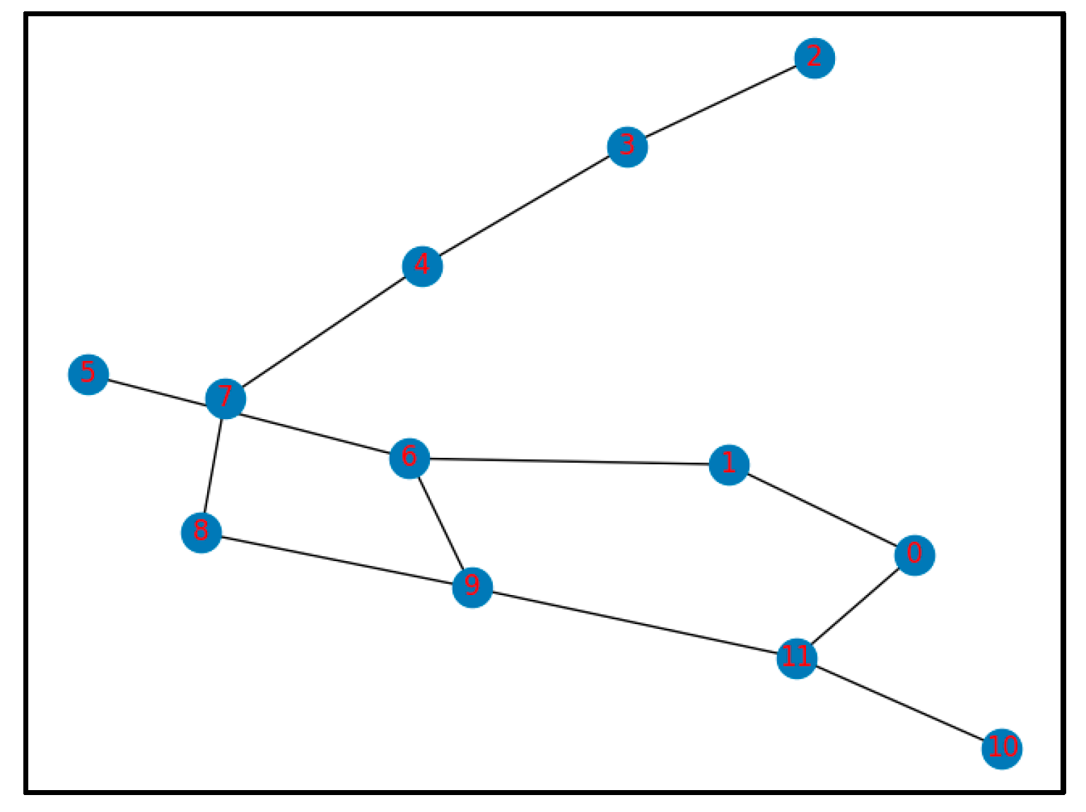
Example 1.

A social network$G\left(V, E\right)$is given, as shown in Figure 1. Firms A and B compete for the opinions of agents in$G\left(V, E\right)$to maximize their own utility. Consider that all other parameters are as follows:$R_A=0.902$,$R_B=0.765$, $C_A=0.260$, $C_B=0.312$, $\gamma =0.717$, $P^0=\left(0.334, 0.805, 0.840, 0.354, 0.625, 0.259, 0.043, 0.088, 0.030, 0.980, 0.715, 0.077\right)$and$\beta =\left(0.609, 0.268, 0.468, 0.049, 0.254, 0.441, 0.793, 0.422, 0.330, 0.424, 0.633, 0.764\right)$. Based on Proposition 1, the equilibrium results are presented in

Table 1. The equilibrium resources received by each agent and expected utilities of firms.

V	v0	v1	v2	v3	v4	v5	v6	v7	v8	v9	v10	v11
$w_i$	0.083	0.044	0.012	0.021	0.035	0.017	0.283	0.045	0.049	0.135	0.027	0.249
$x_i$	0.019	0.006	0.002	0.005	0.008	0.004	0.013	0.004	0.002	0.002	0.005	0.020
$y_i$	0.016	0.005	0.001	0.004	0.007	0.003	0.011	0.003	0.001	0.002	0.004	0.016
$p_i^{200}$	0.307	0.307	0.307	0.307	0.307	0.307	0.307	0.307	0.307	0.307	0.307	0.307
	0.243
$E{U}_B$	0.629

, including the equilibrium resources received by each agent and expected utilities of firms.

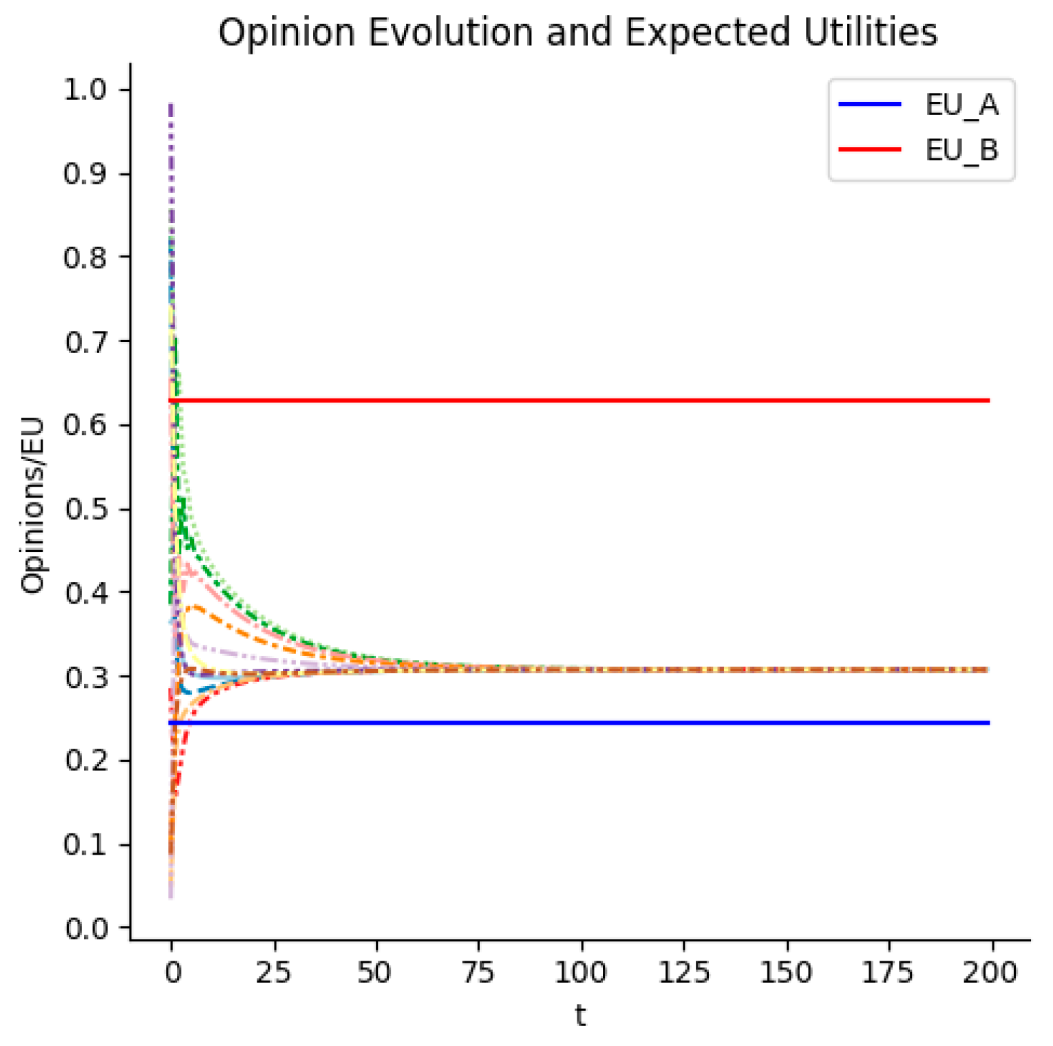
The opinion evolution process and marketing game results are shown in Figure 2.

4.1.2. Equilibrium Results in a Dispersed Network

The equilibrium results of the competition game in a connected network have been presented in Proposition 1. However, the network of consumers may be dispersed and consist of many subnetworks in reality [14]. Furthermore, we want to explore the equilibrium results of the competition game in such a dispersed network.

Assume that the undirected network of agents is dispersed and consists of $m$ disjoint subnetworks, $ℳ=\left\{G_{\left(1\right)}\left(V_{\left(1\right)}, E_{\left(1\right)}, P_{\left(1\right)}^0\right), \cdots , G_{\left(m\right)}\left(V_{\left(m\right)}, E_{\left(m\right)}, P_{\left(m\right)}^0\right)\right\}$. Each subnetwork is path-connected and aperiodic. There exists $P^0=P_{\left(1\right)}^0\cup P_{\left(2\right)}^0\cup \cdots \cup P_{\left(m\right)}^0$ and $V=V_{\left(1\right)}\cup V_{\left(2\right)}\cup \cdots \cup V_{\left(m\right)}$. Lemma 2 implies that agents in each subnetwork can reach a consensus, but different subnetworks engender different resulting opinions (consensuses). We applied a weight vector $ℰ=\left({\epsilon }_1, {\epsilon }_2, \cdots , {\epsilon }_m\right)$ to aggregate the consensuses of each subnetwork $\left(c_1^{\ast }, c_2^{\ast }, \cdots , c_m^{\ast }\right)$ so as to obtain a final consensus of all agents. There was no relationship link between subnetworks. As for the weight vector $ℰ$ among subnetworks, we followed [4,21] to treat it as the form of Equation (24). In our duopoly settings, each agent in the market only had two options, namely firm A or firm B. Firm A will win in the market if more agents favor A, and firm B follows the opposite trend. An agent becomes pivotal for firms if his/her opinion can change the outcome of marketing competition. Let $N$ denote the number of choices firm A needs to win. ${\delta }_i$ denotes the possibility that agent $v_i$ becomes pivotal.

$${\delta }_i={\displaystyle \sum }_{\begin{array}{c}S\subset N\backslash \left\{i\right\}\\ \left|S\right|=N-1\end{array}}{\displaystyle \prod }_{\begin{array}{c}j\in S\\ k\in M\end{array}}{c}_j^{\ast \left(k\right)}{\displaystyle \prod }_{\begin{array}{c}{j}^{\prime }\notin S,j^{\prime }\ne i\\ k^{\prime }\in M\end{array}}\left(1-c_{j^{\prime }}^{\ast \left(k^{\prime }\right)}\right).$$

(23)

$${\epsilon }_k=\frac{1}{\left|V_{\left(k\right)}\right|}{\displaystyle \sum }_{i\in V_{\left(k\right)}}{\delta }_i, \forall k\in ℳ$$

(24)

The equilibrium results of the game in subnetworks are presented in Proposition 2.

Proposition 2.

Given a group of subnetworks$ℳ$, firms A and B both compete for agents’ opinions in these subnetworks to maximize their own utility by competitive expenditure of marketing resources, as in Equations (10) and (11). With the modified budgets$\widehat{R_A}$and$\widehat{R_B}$, the pair of n-vectors$X^{\ast }$ and $Y^{\ast }$ constitute a Nash equilibrium of such a game:

$$\begin{array}{c}{x}_i^{\ast }=\widehat{R_A}\frac{\frac{p_i^0\left(1-p_i^0\right){\left(\widehat{R_B}/\widehat{R_A}\right)}^{\gamma }{w}_i{\epsilon }_k}{{\left[p_i^0+\left(1-p_i^0\right){\left(\widehat{R_B}/\widehat{R_A}\right)}^{\gamma }\right]}^2}}{{\sum }_{i=1}^n\left\{\frac{p_i^0\left(1-p_i^0\right){\left(\widehat{R_B}/\widehat{R_A}\right)}^{\gamma }{w}_i{\epsilon }_k}{{\left[p_i^0+\left(1-p_i^0\right){\left(\widehat{R_B}/\widehat{R_A}\right)}^{\gamma }\right]}^2}\right\}}, i\in V_{\left(k\right)}, k\in ℳ\\ y_i^{\ast }=\widehat{R_B}\frac{\frac{p_i^0\left(1-p_i^0\right){\left(\widehat{R_B}/\widehat{R_A}\right)}^{\gamma }{w}_i{\epsilon }_k}{{\left[p_i^0+\left(1-p_i^0\right){\left(\widehat{R_B}/\widehat{R_A}\right)}^{\gamma }\right]}^2}}{{\sum }_{i=1}^n\left\{\frac{p_i^0\left(1-p_i^0\right){\left(\widehat{R_B}/\widehat{R_A}\right)}^{\gamma }{w}_i{\epsilon }_k}{{\left[p_i^0+\left(1-p_i^0\right){\left(\widehat{R_B}/\widehat{R_A}\right)}^{\gamma }\right]}^2}\right\}}, i\in V_{\left(k\right)}, k\in ℳ\end{array}$$

The equilibrium-expected utility of firm A is

$$E{U}_A={\displaystyle \sum }_{k\in ℳ}{\displaystyle \sum }_{i\in V_{\left(k\right)}}\left\{\frac{p_i^0{\left(\widehat{R_A}\right)}^{\gamma }{w}_i{\epsilon }_k}{p_i^0{\left(\widehat{R_A}\right)}^{\gamma }+\left(1-p_i^0\right){\left(\widehat{R_B}\right)}^{\gamma }}\right\}-C_A\widehat{R_A}.$$

The equilibrium-expected utility of firm B is

$$E{U}_B={\displaystyle \sum }_{k\in ℳ}{\displaystyle \sum }_{i\in V_{\left(k\right)}}\left\{\frac{\left(1-p_i^0\right){\left(\widehat{R_B}\right)}^{\gamma }{w}_i{\epsilon }_k}{p_i^0{\left(\widehat{R_A}\right)}^{\gamma }+\left(1-p_i^0\right){\left(\widehat{R_B}\right)}^{\gamma }}\right\}-C_B\widehat{R_B}.$$

where$w_i=\frac{\frac{\left({\sum }_{j=1, j\ne i}^n{a}_{ij}{d}_j\right)d_i}{1-{\beta }_i}}{{\sum }_{i=1}^n\left\{\frac{\left({\sum }_{j=1, j\ne i}^n{a}_{ij}{d}_j\right)d_i}{1-{\beta }_i}\right\}}$, $\widehat{R_A}=min\left\{R_A, \sum _{k\in ℳ}\sum _{i\in V_{\left(k\right)}}\left\{\frac{\gamma p_i^0\left(1-p_i^0\right){\left(C_A/C_B\right)}^{\gamma }{w}_i{\epsilon }_k}{C_A{\left[p_i^0+\left(1-p_i^0\right){\left(C_A/C_B\right)}^{\gamma }\right]}^2}\right\}\right\}$and$\widehat{R_B}=min\left\{R_B, \sum _{k\in ℳ}\sum _{i\in V_{\left(k\right)}}\left\{\frac{\gamma p_i^0\left(1-p_i^0\right){\left(C_A/C_B\right)}^{\gamma }{w}_i{\epsilon }_k}{C_A{\left[p_i^0+\left(1-p_i^0\right){\left(C_A/C_B\right)}^{\gamma }\right]}^2}\right\}\right\}$.

Proof of Proposition 2.

In the group of subnetworks $ℳ$, the competition game between firms A and B can be written as:

$$\begin{array}{c}\underset{\left\{x_i\right\}}{\max }{\displaystyle \sum _{k\in ℳ}}{\displaystyle \sum _{i\in V_{\left(k\right)}}}\frac{p_i^0{x}_i^{\gamma }}{p_i^0{x}_i^{\gamma }+\left(1-p_i^0\right)y_i^{\gamma }}{w}_i{\epsilon }_k-C_A{\displaystyle \sum _{k\in ℳ}}{\displaystyle \sum _{i\in V_{\left(k\right)}}}{x}_i,\\ \mathrm{s}.\mathrm{t}. {\displaystyle {\sum }_{k\in ℳ}}{\displaystyle {\sum }_{i\in V_{\left(k\right)}}}{x}_i\le R_A.\end{array}$$

(25)

and

$$\begin{array}{c}\underset{\left\{y_i\right\}}{\max }{\displaystyle \sum _{k\in ℳ}}{\displaystyle \sum _{i\in V_{\left(k\right)}}}\frac{\left(1-p_i^0\right)y_i^{\gamma }}{p_i^0{x}_i^{\gamma }+\left(1-p_i^0\right)y_i^{\gamma }}{w}_i{\epsilon }_k-C_B{\displaystyle \sum _{k\in ℳ}}{\displaystyle \sum _{i\in V_{\left(k\right)}}}{y}_i,\\ \mathrm{s}.\mathrm{t}. {\displaystyle {\sum }_{k\in ℳ}}{\displaystyle {\sum }_{i\in V_{\left(k\right)}}}{y}_i\le R_B.\end{array}$$

(26)

Similar to the proof of Proposition 1, we construct the Lagrange functions of Equations (25) and (26) and obtain their respective KKT conditions:

$$A: \{\begin{array}{c}\frac{p_i^0\gamma x_i^{\gamma -1}\left(1-p_i^0\right)y_i^{\gamma }}{{\left[p_i^0{x}_i^{\gamma }+\left(1-p_i^0\right)y_i^{\gamma }\right]}^2}{w}_i{\epsilon }_k-C_A=\lambda \\ {\displaystyle \sum _{k\in ℳ}}{\displaystyle \sum _{i\in V_{\left(k\right)}}}{x}_i\le R_A\\ \lambda \ge 0\\ \lambda \left(R_A-{\displaystyle \sum _{k\in ℳ}}{\displaystyle \sum _{i\in V_{\left(k\right)}}}{x}_i\right)=0\end{array},$$

and

$$B: \{\begin{array}{c}\frac{p_i^0{x}_i^{\gamma }\gamma \left(1-p_i^0\right)y_i^{\gamma -1}}{{\left[p_i^0{x}_i^{\gamma }+\left(1-p_i^0\right)y_i^{\gamma }\right]}^2}{w}_i{\epsilon }_k-C_B=\mu \\ {\displaystyle \sum _{k\in ℳ}}{\displaystyle \sum _{i\in V_{\left(k\right)}}}{y}_i\le R_B\\ \mu \ge 0\\ \mu \left(R_B-{\displaystyle \sum _{k\in ℳ}}{\displaystyle \sum _{i\in V_{\left(k\right)}}}{y}_i\right)=0\end{array}.$$

Similar to the proof of Proposition 1, the solutions are also discussed in four cases. Therefore, we obtain the equilibrium results shown in Proposition 2 from the above KKT conditions. Proposition 2 is proved. □

Proposition 2 indicates that the general weight of each agent consists of the convergence weight in each subnetwork and the weight between subnetworks. Compared with the equilibrium results in a connected network, the equilibrium results in a dispersed network are additionally influenced by the size of the subnetwork and the number of all subnetworks besides some common factors. This may shed light on the market segmentation strategy in marketing decision making.

4.2. Equilibrium Strategies under Different Budgets and Unit Costs

In reality, budget and corresponding resource cost are often the primary factors affecting marketing decisions. There may exist different equilibrium allocation strategies under different budgets and unit costs. This part relaxes the previous assumptions of a fixed budget and given unit cost. Taking the equilibrium results of the connected network as an example, some relevant theoretical and simulation analysis was carried out as follows.

Before starting the analysis, we first give some related definitions.

Definition 1.

As for the competition game shown in Equations (10) and (11), we define the sum of firms’ expected utilities as the expected total utility of the market. Let$TU$denote the expected total utility of the market. Then,

$$TU=E{U}_A+E{U}_B=1-\left(C_A\widehat{R_A}+C_B\widehat{R_B}\right),$$

(27)

where$\widehat{R_A}$and$\widehat{R_B}$are denoted as before. Obviously, a low unit cost of each firm means the total utility of the market will be high.

Definition 2.

As for the competition game shown in Equations (10) and (11), we define the difference between firms’ expected utilities as the outcome of the competition game. Let$S$denote the competition outcome. Then,

$$S=E{U}_A-E{U}_B={\displaystyle \sum }_{i=1}^n\left\{\frac{p_i^0{\left(\widehat{R_A}\right)}^{\gamma }-\left(1-p_i^0\right){\left(\widehat{R_B}\right)}^{\gamma }}{p_i^0{\left(\widehat{R_A}\right)}^{\gamma }+\left(1-p_i^0\right){\left(\widehat{R_B}\right)}^{\gamma }}{w}_i-C_A\widehat{R_A}+C_B\widehat{R_B}\right\}.$$

(28)

Explicitly,$S>0$means firm A will win the competition in the market, and$S<0$means firm B will win the competition in the market.

4.2.1. The Effect of Unit Costs on Equilibrium Strategies

Based on Equations (27) and (28), we have their FOCs as below:

$$\frac{\partial TU}{\partial C_A}=-\widehat{R_A}<0, \frac{\partial TU}{\partial C_B}=-\widehat{R_B}<0; \frac{\partial S}{\partial C_A}=-\widehat{R_A}<0, \frac{\partial S}{\partial C_B}=\widehat{R_B}>0$$

(29)

Applying the FOCs to Equations (14) and (15), we then have

$$\frac{\partial E{U}_A}{\partial C_A}=-\widehat{R_A}<0, \frac{\partial E{U}_B}{\partial C_B}=-\widehat{R_B}<0$$

(30)

We found that the expected utility of each firm decreases monotonically with its unit cost (see Equation (30)). If the unit cost is reduced, then each firm can not only improve its expected utility but also improve the total utility of the market (see Equations (29) and (30)). Therefore, efforts to reduce costs are necessary for each firm in the market. Given other conditions, each firm can judge its possibility of winning the competition and determine its allocation strategy according to its unit cost and that of the opponent. Furthermore, each firm can derive the minimum reduction in unit cost from the definition of competition outcome so that it can win in the market (see Equation (28)).

Additionally, we applied a small-world network to simulate the consumer network in a market. Assume that the consumer network consists of 12 agents, whose initial opinions and self-belief are all generated stochastically in the range of $\left(0, 1\right)$. The efficiency parameter $\gamma$ of each firm is equal and is also generated stochastically in the range of $\left(0, 1\right)$. The unit costs of firms A and B both vary in the scope of $\left[0.05, 0.1, 0.15, 0.2, 0.25, 0.3, 0.35, 0.4, 0.45, 0.5, 0.55, 0.6, 0.65, 0.7, 0.75, 0.8, 0.85, 0.9, 0.95\right]$. Define the marketing resource ratio at equilibrium (RRE) as $RRE=y_i^{\ast }/x_i^{\ast }$. Given the budgets of firms A and B, the simulation results of competition outcome $S$ and the RRE are presented below.

From Figure 3, we found that the competition outcome $S$ increased monotonically with $C_B$ and decreased monotonically with $C_A$, which is in line with the FOCs shown in Equation (29). The competition outcome was more sensitive to the change of firm B’s unit cost in the case of $R_A=0.2, R_B=0.8$, while the competition outcome was more sensitive to the change of firm A’s unit cost in the case of $R_A=0.8, R_B=0.2$. For the case of $R_A=R_B=0.5$, the unit cost of each firm had a symmetrical effect on the competition outcome. Moreover, according to Proposition 1, the value of the RRE determines the equilibrium-expected utilities of firms A and B, and $RRE=\left\{R_B/R_A, C_A/C_B\right\}$. Figure 3 implies that the RRE will take the value of $C_A/C_B$ if unit costs of firms A and B are both high enough. Conversely, the RRE will take the value of $R_B/R_A$ if the unit costs of firms A and B are both low enough. In other words, the level of unit cost affects the equilibrium results by influencing the value of the RRE. High unit costs hinder the enthusiasm of firms to allocate budgets, while low unit costs promote firms to use up their budgets as much as possible.

4.2.2. The Effect of Budgets on Equilibrium Strategies

The modified budget can be interpreted as the total marketing resources that are actually allocated among agents. According to Proposition 1, the modified budget represents the budget to some extent. Then, we have the FOCs from Equations (27) and (28):

$$\frac{\partial TU}{\partial \widehat{R_A}}=-C_A<0, \frac{\partial TU}{\partial \widehat{R_B}}=-C_B<0$$

(31)

$$\begin{gathered} \frac{\partial S}{\partial \widehat{R_A}}={\displaystyle \sum }_{i=1}^n\frac{2\gamma p_i^0\left(1-p_i^0\right){\widehat{R_A}}^{\gamma -1}{\widehat{R_B}}^{\gamma }}{{\left[p_i^0{\widehat{R_A}}^{\gamma }+\left(1-p_i^0\right){\widehat{R_B}}^{\gamma }\right]}^2}{w}_i-C_A, \\ \frac{\partial S}{\partial \widehat{R_B}}={\displaystyle \sum }_{i=1}^n\frac{-2\gamma p_i^0\left(1-p_i^0\right){\widehat{R_A}}^{\gamma }{\widehat{R_B}}^{\gamma -1}}{{\left[p_i^0{\widehat{R_A}}^{\gamma }+\left(1-p_i^0\right){\widehat{R_B}}^{\gamma }\right]}^2}{w}_i+C_B. \end{gathered}$$

(32)

Applying the FOCs to Equations (14) and (15), then there are

$$\begin{gathered} \frac{\partial E{U}_A}{\partial \widehat{R_A}}={\displaystyle \sum }_{i=1}^n\frac{\gamma p_i^0\left(1-p_i^0\right){\widehat{R_A}}^{\gamma -1}{\widehat{R_B}}^{\gamma }}{{\left[p_i^0{\widehat{R_A}}^{\gamma }+\left(1-p_i^0\right){\widehat{R_B}}^{\gamma }\right]}^2}{w}_i-C_A, \\ \frac{\partial E{U}_B}{\partial \widehat{R_B}}={\displaystyle \sum }_{i=1}^n\frac{\gamma p_i^0\left(1-p_i^0\right){\widehat{R_A}}^{\gamma }{\widehat{R_B}}^{\gamma -1}}{{\left[p_i^0{\widehat{R_A}}^{\gamma }+\left(1-p_i^0\right){\widehat{R_B}}^{\gamma }\right]}^2}{w}_i-C_B. \end{gathered}$$

(33)

From Equation (31), we found that the total utility of the market gradually decreases with the increase resources actually spent. However, according to Equations (32) and (33), the competition outcome and the utility of each firm are not monotonic on each modified budget, that is, they are not monotonic on each budget. Additionally, there may exist a certain modified budget that makes the corresponding expected utility reach its maximum. Numerical simulations show this more intuitively.

Consider the same small-world network as above. Initial opinions, self-belief and the efficiency parameter are all generated stochastically in the range of $\left(0, 1\right)$. Given the unit costs of firms A and B, the budgets of each firm both vary in the scope of $\left[0.05, 0.1, 0.15, 0.2, 0.25, 0.3, 0.35, 0.4, 0.45, 0.5, 0.55, 0.6, 0.65, 0.7, 0.75, 0.8, 0.85, 0.9, 0.95\right].$ The simulation results of competition outcome $S$ and the RRE are shown in Figure 4.

As Figure 4 shows, the effect of budgets on the competition outcome is quite complex and non-monotonic, which is consistent with the FOCs shown in Equation (32). By comparing Figure 2a–c, we found that a firm with a low unit cost dominates the competition. The budget has a very limited effect on reversing the competition outcome when there is a great disparity in unit costs between firms. As seen in each subgraph of Figure 4, the change of budgets can only have a large impact on the competition outcome if there is a disparity between the budgets of firms A and B. For a given budget of the opponent, each firm can assess its chances of winning and optimally adjust its own budget to ensure a win based on Equation (28). Furthermore, such an adjustment is not unique due to the non-monotonicity of the effect. Each firm can take advantage of the non-uniqueness to make a minimal budget adjustment for a win.

Specifically, these characteristics of the effect on the competition outcome can be understood in terms of the trend of the RRE, because the value of the RRE determines the equilibrium results to some extent. We found that the value of the RRE is taken as $C_A/C_B$ when the budgets of both firms are large enough; otherwise it is taken as $R_B/R_A$. When the value of the RRE is $C_A/C_B$, the competition outcome $S$ can be rewritten as

$$S={\displaystyle \sum }_{i=1}^n\frac{p_i^0-\left(1-p_i^0\right){\left(C_A/C_B\right)}^{\gamma }}{p_i^0+\left(1-p_i^0\right){\left(C_A/C_B\right)}^{\gamma }}{w}_i.$$

From the above equation, we found the competition outcome is only determined by the network structure and initial opinions for a given pair of unit costs. Thus, the competition outcome does not change with budgets of firms A and B, as shown in Figure 4. As for the case of $C_A=C_B=0.5$, the fluctuation in the upper-right part of Figure 4b was caused by the stochasticity of network structure and initial opinions in the simulations, rather than the change of budgets.

4.3. Equilibrium Strategies under Different Network Structures

From Proposition 1, strategic allocation decision is made based on opinion evolution, and the opinion evolves based on social relations in the network. Therefore, there may exist different equilibrium strategies under different network structures. Consider a group of 12 agents, the social relations between whom are generated stochastically in the form of small-world networks. Likewise, budgets, unit costs, self-belief, initial opinions and the efficiency parameter are all generated stochastically in the range of $\left(0, 1\right)$. Additionally, we considered another case where there are no social connections among agents. By comparing the two cases of agents with and without connections, we can have an intuitive understanding of the effect of network structure. The comparison is shown in Figure 5.

Since the relationships between agents are diverse, there are many possible structures for the network. From Figure 5, the diversity of network structures allows for multiple possible results for each firm’s expected utility. Expected utilities of firms in the case of agents with connections may be greater than or less than those in the case of agents without connections. For both sides of the competition in the market, the network structure may be used as a tool to improve utilities.

Inspired by Stewart et al. [24], we applied a novel notion, the network dominance gap (NDG), to exquisitely characterize the heterogeneous advantages of network structures to different firms. We can gain a glimpse of the role of network structure in equilibrium strategies from the NDG, which is defined as follows.

Definition 3.

Given a social network$G\left(V, E\right)$defined as before, let$V_i$denote the set of neighbors of agent$v_i$, $V_i=\left\{j\in V|a_{ij}=1\right\}$. Agents in the network hold heterogeneous initial opinions, namely$\left(p_1^0, p_2^0, \cdots , p_n^0\right)$. $d_i$is denoted as before. Then, the dominance of$v_i$for firm A is

$${\mathcal{G}}_i^A={\displaystyle \sum }_{j\in V_i}\left(p_j^0\times \frac{d_j}{{{\displaystyle \sum }}_{k\in V_i}{d}_k}\right).$$

The dominance of$v_i$for firm B is

$${\mathcal{G}}_i^B={\displaystyle \sum }_{j\in V_i}\left[\left(1-p_j^0\right)\times \frac{d_j}{{{\displaystyle \sum }}_{k\in V_i}{d}_k}\right].$$

Then, the NDG labeled by$\mathcal{G}$is

$$\mathcal{G}={\displaystyle \sum }_{i=1}^n\left({\mathcal{G}}_i^A-{\mathcal{G}}_i^B\right)={\displaystyle \sum }_{i=1}^n\left\{\frac{{\sum }_{j\in V_i}\left(2p_j^0-1\right)d_j}{{\sum }_{j\in V_i}{d}_j}\right\}.$$

From Definition 3, $\mathcal{G}>0$ means that most agents in the network are surrounded by supporters of firm A. Thus, most agents in the network meet the condition that the majority of their neighbors are supporters of firm A. Therefore, $\mathcal{G}>0$ indicates that this network has an innate dominance for firm A. Then, $\mathcal{G}<0$ indicates that this network has an innate dominance for firm B. What the NDG stresses is the innate network dominance before opinion evolution, not the final dominance. In the process of opinion evolution, this innate dominance is affected by other factors, such as self-belief, external resources and unit costs. So, will this network dominance run through the whole evolution process and be retained in equilibrium? Numerical simulations give a preliminary answer.

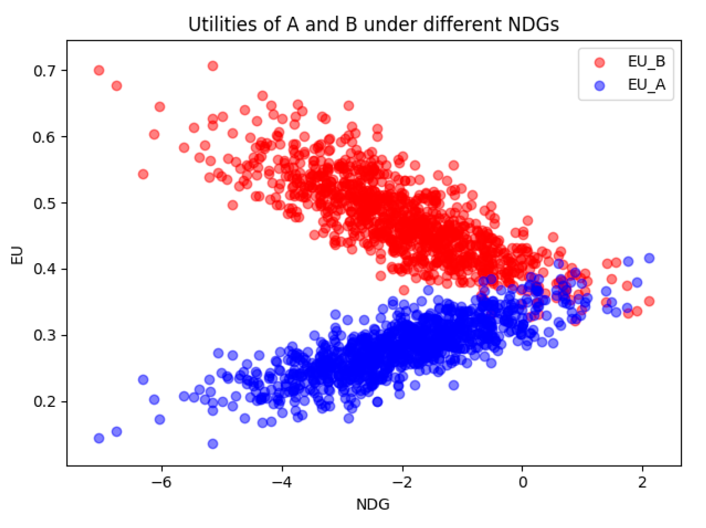
For the same group of agents as Figure 5, the social relations between them are generated stochastically in the form of small-world networks. All parameters are the same, as given in Figure 5. Then, the relationship between the NDG and the expected utility of each firm is shown in Figure 6.

From Figure 6, the expected utility of firm A is positively correlated with the NDG, while the expected utility of firm B is negatively correlated with the NDG. Obviously, the network dominance is retained in equilibrium and manifested in the expected utility of each firm. A positive and large NDG often means that the network has an advantage for the marketing campaign of firm A, i.e., $E{U}_A$ is generally greater than $E{U}_B$, while a negative and small NDG means that $E{U}_A$ is generally less than $E{U}_B$. For any given initial opinion profile, the NDG implies that the difference between expected utilities of firm A and B varies continuously under different network structures. Consequently, the structure of a network can indeed be used as a tool for firms to improve their expected utilities, which is in line with [12,25]. Therefore, it is quite necessary for firms in the market to investigate the consumer network and improve its structure accordingly. Meanwhile, each firm can choose its optimal marketing strategy under different network structures.

5. Conclusions

This paper has investigated the problem of competitive marketing resource allocation under cost and budget constraints. We modeled the allocation competition as a non-zero-sum game, where two firms attempt to compete for consumers’ opinions to maximize their own utilities in a market. In the constructed model, a bridge is built between the inner state (self-belief and opinions) of consumers and allocation decisions of firms in the game. Thus, the allocation of marketing resources is targeted and based on dynamic opinions of consumers in networks, which provides a meaningful feedback loop between consumers and firms in the market. In general, the main conclusions can be summarized as follows.

• Combining opinion dynamics and game theory for allocation decisions of marketing resources, we constructed a novel hybrid model to characterize how firms target their marketing resources to consumers in social networks under cost and budget constraints.
• From the constructed model, we obtained its equilibrium results in the form of theoretical expressions in a connected network and a dispersed network, which provided a sharp and apt characterization of the marketing resource allocation strategies.
• Through discussing the properties of equilibria, we can determine that firms should allocate more marketing resources to some of consumers with certain characteristics. As for initial opinions, firms should allocate more resources to the consumer whose initial opinion is close to ${\widehat{R_B}}^{\gamma }/\left({\widehat{R_A}}^{\gamma }+{\widehat{R_B}}^{\gamma }\right)$. As for self-belief, firms should allocate more resources to consumers with high self-belief. As for the position in a network, firms should allocate more resources to consumers with many neighbors whose neighbors are also numerous. All of these provide some implications for marketing resource management.
• By relaxing some fixed parameters, we found that the expected utility of each firm decreases monotonically with its unit cost and is not monotonic on its budget. The competition outcome is more sensitive to the change of unit cost of a firm with a relatively small budget and can reach its extremum at some value of the budget. These imply that reducing the unit cost of marketing is quite essential and that “the more the better” rule does not apply to a firm’s marketing budget. Moreover, the network may have an innate dominance for one of the firms in the market competition, and network structure can be as a tool to improve the firm’s utility. These findings provide some reference and implications for firms in marketing competition.

Despite the above contributions, this paper still has some limitations, such as difficulties in analyzing the competition of multiple players or modeling a dynamic multi-stage marketing process. Additionally, there may be negative relationships among agents in networks, which can hinder the effect of marketing campaigns [26]. Consequently, it is necessary to explore the problem of marketing competition in a signed network. These limitations are the focus of our future research. In future research, we plan to further study such an allocation competition in a dynamic game or in a signed network. Undoubtedly, dynamic games and signed networks make the competition model closer to the actual marketing competition in social networks [26,27,28]. Corresponding allocation strategies will make sense and be of great interest.

References

- Bimpikis, K.; Ozdaglar, A.; Yildiz, E. Competitive Targeted Advertising over Networks. Oper. Res. 2016, 64, 705–720. [Google Scholar] [CrossRef]
- Dong, Y.; Chen, X.; Hunt, K.; Zhuang, J. Defensive Resource Allocation: The Roles of Forecast Information and Risk Control. Risk Anal. 2021, 41, 1304–1322. [Google Scholar] [CrossRef] [PubMed]
- Friedman, L. Game-Theory Models in the Allocation of Advertising Expenditures. Oper. Res. 1958, 6, 699–709. [Google Scholar] [CrossRef]
- Snyder, J.M. Election Goals and the Allocation of Campaign Resources. Econometrica 1989, 57, 637–660. [Google Scholar] [CrossRef]
- Li, J.; Ni, X.; Yuan, Y.; Wang, F.-Y. A hierarchical framework for ad inventory allocation in programmatic advertising markets. Electron. Commer. Res. Appl. 2018, 31, 40–51. [Google Scholar] [CrossRef]
- Tavasoli, A.; Shakeri, H.; Ardjmand, E.; Young, W.A. Incentive rate determination in viral marketing. Eur. J. Oper. Res. 2021, 289, 1169–1187. [Google Scholar] [CrossRef]
- Bimpikis, K.; Ehsani, S.; İlkılıç, R. Cournot Competition in Networked Markets. Manag. Sci. 2019, 65, 2467–2481. [Google Scholar] [CrossRef]
- Kovenock, D.; Roberson, B. Generalizations of the General Lotto and Colonel Blotto games. Econ. Theory 2020, 71, 997–1032. [Google Scholar] [CrossRef]
- Yin, X.; Wang, H.; Yin, P.; Zhu, H. Agent-based opinion formation modeling in social network: A perspective of social psychology. Phys. A Stat. Mech. Appl. 2019, 532, 121786. [Google Scholar] [CrossRef] [Green Version]
- Zha, Q.; Dong, Y.; Chiclana, F.; Herrera-Viedma, E. Consensus Reaching in Multiple Attribute Group Decision Making: A Multi-Stage Optimization Feedback Mechanism with Individual Bounded Confidences. IEEE Trans. Fuzzy Syst. 2021. [Google Scholar] [CrossRef]
- Zha, Q.; Kou, G.; Zhang, H.; Liang, H.; Chen, X.; Li, C.-C.; Dong, Y. Opinion dynamics in finance and business: A literature review and research opportunities. Financ. Innov. 2021, 6, 44. [Google Scholar] [CrossRef]
- Morărescu, I.C.; Varma, V.S.; Buşoniu, L.; Lasaulce, S. Space–time budget allocation policy design for viral marketing. Nonlinear Anal. Hybrid Syst. 2020, 37, 100899. [Google Scholar] [CrossRef]
- Kaiser, C.; Kröckel, J.; Bodendorf, F. Simulating the spread of opinions in online social networks when targeting opinion leaders. Inf. Syst. E-Bus. Manag. 2012, 11, 597–621. [Google Scholar] [CrossRef]
- Zaglia, M.E. Brand communities embedded in social networks. J. Bus. Res. 2013, 66, 216–223. [Google Scholar] [CrossRef]
- Varma, V.S.; Lasaulce, S.; Mounthanyvong, J.; Morarescu, I.-C. Allocating Marketing Resources Over Social Networks: A Long-Term Analysis. IEEE Control Syst. Lett. 2019, 3, 1002–1007. [Google Scholar] [CrossRef] [Green Version]
- Agieva, M.T.; Korolev, A.V.; Ougolnitsky, G.A. Modeling and Simulation of Impact and Control in Social Networks with Application to Marketing. Mathematics 2020, 8, 1529. [Google Scholar] [CrossRef]
- Zha, Q.; Dong, Y.; Zhang, H.; Chiclana, F.; Herrera-Viedma, E. A Personalized Feedback Mechanism Based on Bounded Confidence Learning to Support Consensus Reaching in Group Decision Making. IEEE Trans. Syst. Man Cybern. Syst 2021, 51, 3900–3910. [Google Scholar] [CrossRef] [Green Version]
- Zha, Q.; Liang, H.; Kou, G.; Dong, Y.; Yu, S. A Feedback Mechanism With Bounded Confidence- Based Optimization Approach for Consensus Reaching in Multiple Attribute Large-Scale Group Decision-Making. IEEE Trans. Comput. Soc. Syst. 2019, 6, 994–1006. [Google Scholar] [CrossRef]
- Degroot, M.H. Reaching a Consensus. J. Am. Stat. Assoc. 1974, 69, 118–121. [Google Scholar] [CrossRef]
- Skaperdas, S. Contest success functions. Econ. Theory 1996, 7, 283–290. [Google Scholar] [CrossRef]
- Guzmán, C. Strategic Competitions over Networks; Stanford University: Stanford, CA, USA, 2010. [Google Scholar]
- Freeman, L.C. Centrality in social networks conceptual clarification. Soc. Netw. 1978, 1, 215–239. [Google Scholar] [CrossRef] [Green Version]
- Ding, Z.; Chen, X.; Dong, Y.; Herrera, F. Consensus reaching in social network DeGroot Model: The roles of the Self-confidence and node degree. Inf. Sci. 2019, 486, 62–72. [Google Scholar] [CrossRef]
- Stewart, A.J.; Mosleh, M.; Diakonova, M.; Arechar, A.A.; Rand, D.G.; Plotkin, J.B. Information gerrymandering and undemocratic decisions. Nature 2019, 573, 117–121. [Google Scholar] [CrossRef]
- Dong, Y.; Zha, Q.; Zhang, H.; Herrera, F. Consensus Reaching and Strategic Manipulation in Group Decision Making With Trust Relationships. IEEE Trans. Syst. Man Cybern. Syst. 2021, 51, 6304–6318. [Google Scholar] [CrossRef]
- He, Q.; Sun, L.; Wang, X.; Wang, Z.; Huang, M.; Yi, B.; Wang, Y.; Ma, L. Positive opinion maximization in signed social networks. Inf. Sci. 2021, 558, 34–49. [Google Scholar] [CrossRef]
- Gelper, S.; van der Lans, R.; van Bruggen, G. Competition for Attention in Online Social Networks: Implications for Seeding Strategies. Manag. Sci. 2021, 67, 1026–1047. [Google Scholar] [CrossRef]
- Yang, L.-X.; Li, P.; Yang, X.; Xiang, Y.; Tang, Y.Y. Simultaneous Benefit Maximization of Conflicting Opinions: Modeling and Analysis. IEEE Syst. J. 2020, 14, 1623–1634. [Google Scholar] [CrossRef]
Figure 1.
The social network.
Figure 2.
The opinion evolution process and expected utilities of firms A and B.
Figure 3.
Average competition outcomes and average RREs of 1000 simulations under different unit costs and different pairs of budgets: (a) ; (b) ; and (c) .
Figure 4.
Average competition outcomes and average RREs of 1000 simulations under different budgets and different pairs of unit costs: (a) ; (b) ; and (c) .
Figure 5.
Expected utilities of firms in the cases of agents with and without connections.
Figure 6.
The relationship between the NDG and the expected utility of each firm.