Equilibrium in a Queueing System with Retrials

Abstract

We find an equilibrium in a single-server queueing system with retrials and strategic timing of the customers. We consider a set of customers, each of which must decide when to arrive to a queueing system during a fixed period of time. In this system, after completion of service, the server seeks a customer blocked in a virtual orbit (orbital customer) to be served next, unless a new customer captures the server. We develop, in detail, a setting with two and three customers in the set, and formulate and discuss the problem for the general case with an arbitrary number of customers. The numerical examples for the system with two and three customers included as well.

1. Introduction

The retrial queues have been attracting increasing interest because of their importance in modeling modern wireless telecommunication systems. Many papers have been devoted to steady-state performance analysis of such queues with the most important sources mentioned here [1,2,3]. Firstly, we outline the main settings that describe the dynamics of a wide class of the retrial queueing systems.

There are many practical situation that can be modeled as a queueing system in which customers are allowed to have a few attempts to be served. For instance, in call centers with a callback option, as well as customers who cannot connect immediately with the operator, thus register their numbers and go back at a later time. These customers can be called orbital because it seems natural that registered customers are waiting for service in a so-called orbit-queue (orbit). As these customers cannot be picked up immediately when the operator becomes available, some seeking time (called retrieval time) is needed to access a registered customer. We note that sometimes the operator may make an outgoing call, not being aware of the presence of the registered customers in the orbit. A similar situation (with retrial attempts) arises in many service systems where a ticket is issued upon the arrival of a customer who will be served in a later time when the server is available.

Now we touch upon service disciplines that are considered in the retrial queueing systems. The most traditional discipline is the so-called classical retrials, when the customers blocked in the orbits make retrial attempts independently, in which case the retrial rate increases (linearly) as the orbit size increases. Stability analysis of such systems are considered in the mentioned books (mainly in the Markovian setting), and in a more general setting, this analysis has been performed in the papers [4,5,6].

The latter approach, in a generalized form, has been applied to the stability analysis of a wide class of queueing systems (including many retrial systems) in the recent book [7]. The main ingredient of the analysis is to establish the negative drift of the remaining work (workload) when the orbit size becomes large. Moreover, a key observation is that, from the point-of-view of stability, such a retrial system approaches the classic buffered system when the orbit size increases unlimitedly. (We call it an asymptotically work-conserving discipline in [5].) The following step to simplify the regenerative stability analysis has been realized in the paper [6], in which the positive drift of the idle time of the servers is used (instead of the positive drift of the workload) under the assumption that the orbit size increases to infinite in probability. (For more on regenerative stability analysis, see [7].)

Another wide and important class of the retrial models is the queueing systems with the constant retrial rate, see Chapter 7 in [7]. These models play an important role in the analysis of modern wireless telecommunication systems. In this regard, we mention the paper [8] in which, to the best of our knowledge, such a model has been used for the first time to model a telephone exchange system. A retrial queueing system with a constant retrial rate is suitable to describe the behavior of the multiple access protocols [9]. The retrial queues with a constant retrial rate have been applied to model TCP (Transmission Control Protocol) traffic related to short HTTP (HyperText Transfer Protocol) connections and to describe an optical-electrical hybrid contention resolution scheme [10]. There is also a modification of the retrial system in which, after each departure, the server seeks the customer in orbit (this is the above-mentioned retrieval time) to be served next. For instance, such a system has been considered in the paper [11], where a logarithmic asymptotic of a large deviation probability of the orbit size during the regeneration period is obtained. Moreover, in this paper we also consider the system with the retrieval time.

The most interesting and newest setting related to a retrial system is the so-called retrial systems with coupled orbits [12], which have potential applications to model the wireless multiple access systems. In particular, they can model the relay-assisted cognitive cooperative wireless systems in which the users transmit packets to a common destination node, and there are a finite number of relay nodes (i.e., orbits) that assist to retransmit the blocked packets; when a direct source user transmission is blocked, it forwards the blocked packet at a relay node [13]. Recent progress in the analysis of the queueing systems with coupled orbits is presented in book [7]. (See Chapters 7–9, where motivation and further references can be also found.)

Among the most important previous results in the analysis of the retrial systems, we mention the explicit expression for the stationary remaining service time of the server, which has been obtained in the recent paper [14]. It is easy to show that this result is also applicable for the stationary retrial queueing system. The mentioned result has a potential application in the setting in which the customers (both in the input process and in orbit) can select the instant to capture the server. An analysis of such a setting is very close to the main purpose of present paper. In the context of the present paper, it is important to emphasize that in the conventional queueing theory setting, customers following an input process are unable to make their own decision, while now we allow this possibility. To best of our knowledge, this setting is completely new, and this is the main contribution of our paper.

In conventional queueing theory, the structure of the input process and service process are usually assumed to be predefined and specified by the input rate and service times of the customers. However, there exists a different approach to the queueing which is based on the assumption that the customers (or users) logging into the system are strategic ([15,16,17,18,19,20,21,22,23,24,25]). Namely, it is assumed that the user strategy is to select the arrival instant to the system on a time interval $[0,T]$. In this setting, the queue in the system is determined after each player selects (at the initial instant $t=0$) their random arrival instant in the system. Thus, each user spends some time in the system, and this time is their personal utility function. As a result, a non-zero-sum game is obtained, in which we need to find the Nash equilibrium. To the best of our knowledge, the paper [15] (by Glazer and Hassin) is the first work that considers the queue as a result of the user’s behavior, and the authors denote this system as $?/M/1$. They further formulate a non-cooperative game in which a Poisson-distributed number of the customers determines their arrival instances in the queue of a single-server system, over a (limited) admission interval $[0,T]$. The purpose of the customers is to minimize their waiting time in the system. It is shown in [15] that the symmetric Nash equilibrium strategy is mixed. In particular, it was revealed that this strategy is the (absolutely continuous) uniform distribution over time interval $[0,T]$, except a singularity at zero, and the density function decreases between zero and T. A similar model $?/M/m/c$ with $m\ge 1$ identical (exponential) servers and the buffer size $c\ge 0$ for the waiting customers is considered in the paper [22]. Note that the arrival times game with the batch service has been investigated in [16]. A single-server bufferless system in which the customers have a time-sensitivity function that they want to minimize, instead of their own waiting costs, has been studied in [18]. The paper [20] establishes conditions under which the customers cannot queue until an opening time, and shows that, in the equilibrium, there is a singularity at instant $t=0$, and that the density is positive only since an instant $t_e>0$. A model where the customers may incur tardiness costs in addition to the waiting costs is considered in [21]. The paper [25] considers a model combining the tardiness costs, waiting costs, and restrictions on the opening and closing times. (An overview of the existing literature on this problem can also be found in [25].)

In this paper, we apply a game-theoretic approach to a callback queueing system with one server. The queue is formed by the strategic players. (In what follows, we use the terms ‘customer’, ‘user’, and ‘players’ as synonyms.) The player’s strategy is to choose a moment to enter the system. If the server is busy, then the user is blocked and joins a (virtual) orbit queue. Otherwise, if the server is free, it seeks a blocked user from the orbit during an (exponential) retrieval time. In this setting, we will find the optimal strategies of the players. First, we consider the case of two users, then consider in detail the case of three players and finally formulate this problem for an arbitrary number of players.

Thus, the found optimal strategies of the players in the described retrial system is the main contribution of this paper.

The paper is organized as follows. In Section 2, we describe the model in details. Then in Section 3, we study the setting with two players. The simplest setting allows one to highlight the main ideas and steps of our analysis. In Section 4, we focus on the system with three players, and the analysis in this case turns out to be much more involved. The analysis of the game with three players is continued in Section 5 where an algorithm on how to find an approximation of the equilibrium is given. The developed approach is then extended to a general setting with $N+1$ players in Section 6. Moreover, we consider a few numerical examples in Section 3 and Section 6.

2. Description of the Model

Now we describe our model in more details in a general setting. We assume that there exists a single server that serves N (‘exogenous’) customers presented in the system at the initial instant $t=0$. Unlike the conventional queueing theory setting, these customers use some strategy to choose an instant to enter the server. By a symmetry, this strategy is the same for each user. This strategy is determined by a distribution function, which is the main purpose of the analysis, and it determines the instant of the attempt to enter the server, see (1) below. This is an important difference with the standard queueing theory setting where customers are not allowed to have their own decisions but follow the predefined rules describing the dynamics of the system. After the departure of a served customer, the server starts to seek the customer blocked in orbit (if any) to be served next. As mentioned above, this seeking time is exponential with parameter $\gamma$ and mean $\tau$, and it is called retrieve time in the retrial queueing terminology [11]. If an exogenous customer finds a server busy, then they join a (virtual) orbit, and such orbital customers constitute a virtual orbit queue (see [12]), which is served in FIFO (First-In-First-Out) order. If, during a retrieval time (when the server is idle), some customer arrives then they capture server for the exponentially distributed time with parameter $\mu$. Recall that the arrival time is selected in according to distribution (1). Thus, the present setting combines some features of both the classic retrial system and a gated queue, in which the input gate remains closed until all N customers leave the system. In addition, a similar situation arises in a polling system (see, for instance, [26]), in which different queues are served in an order, and server, returning to a fixed queue, as a rule finds there a few new customers to be served.

Remark 1.

In our setting, the system has initially a finite number of players, and in this case the system is stable in a traditional sense: The number of customers is bounded. However, in our analysis the requirement $\mu >\gamma$ on the parameters μ and γ appears (see (8)), which indeed can be treated as a stability condition in the framework of the considered game setting. Moreover, when the number of players is N (see Section 6) then the classic stability analysis could be critically important in the asymptotic setting as $N\to \infty$.

3. Two Players Scenario

Consider the case of two players. To find an equilibrium in this two-person game, we will use the following approach. Suppose that one of the players (for the sake of definiteness, the second player) uses, as a strategy, a random arrival time with the distribution function $F\left(t\right)$ (having density $f\left(t\right)$) of the following form:

$$F\left(t\right)=\left\{\begin{array}{c}p,0\le t<t_e,\hfill \\ p+{\int }_{t_e}^{t}f\left(x\right)dx,t_e\le t\le T.\hfill \end{array}\right.$$

(1)

That is, the second player enters the system at the initial moment $t=0$ with probability $p\in (0,1)$, otherwise, they arrive at instant $t\in [t_e,T]$ following distribution $F\left(t\right)$, where $t_e>0$ and $T<\infty$ are predefined constants.

Now, we find the best response of the first player to the described strategy used by the second player. As a cost function of the first player, we will consider their average sojourn time (the average time the player spends in the system). Thus, the objective of the first player is to choose a strategy that minimizes the average sojourn time, that is the total time the player spends in the system. Due to the symmetry of the problem, in the equilibrium, the optimal strategy of the first player must coincide with the chosen strategy of their opponent. To do this, it is sufficient that the strategy of the second player is chosen in such a way that the cost function of the first player takes a constant value over the interval $[t_e,T]$ and at the initial instant $t=0$ (see [24]). Then the payoff of the first player will not depend on their own strategy.

Next, we find the best response of the first player to the strategy of the second player defined by the relation (1). First, we find its cost function. The average sojourn time, provided the first player enters the system at the instant $t=0$, is:

$$C\left(0\right)=(1-p)\frac{1}{\mu }+p(\frac{1}{2}\frac{1}{\mu }+\frac{1}{2}(\tau +\frac{2}{\mu }))=(1-p)\frac{1}{\mu }+p(\frac{3}{2\mu }+\frac{\tau }{2}).$$

In this expression, we take into account that, with the probability $1-p$, the second player does not arrive in the system at the instant $t=0$. Then the first player will be served first, and the average sojourn time equals the average service time $1/\mu$. If the second player arrives at the instant $t=0$ (with the probability p), then, with probability $1/2$, the first player can be selected for service, and their average service time equals $1/\mu$. However, with probability $1/2$, the server chooses the second player, and then the first player joins the orbit and waits until the second player ends service.

If $0<t<t_e$, then the average sojourn time of a customer that arrives at instant t satisfies:

$$\begin{array}{cc}\hfill C\left(t\right)& =(1-p)\frac{1}{\mu }+p\left((1-e^{-\mu t})\frac{1}{\mu }+e^{-\mu t}(\frac{1}{\mu }+\tau +\frac{1}{\mu })\right)\hfill \\ & =(1-p)\frac{1}{\mu }+p\left(\frac{1}{\mu }+e^{-\mu t}(\tau +\frac{1}{\mu })\right).\hfill \end{array}$$

To obtain this expression, we take into account that, with the probability $1-p$, the second player does not arrive at instant $t=0$. In this case, the first player is served first, and the average (sojourn) service time equals $1/\mu$. If the second player arrives at $t=0$ (with the probability p), then with probability $1-exp\{-\mu t\}$, it will be served in the time interval $[0,t]$, and then the first player will be served immediately. However, with the probability $exp\{-\mu t\}$, the second player is still in the server at instant t, and then the first player joins the orbit. This player will wait until the second player leaves the server, and then they occupy server after time $\tau$. We note that function $C\left(t\right)$ decreases in t and then, in the limit as $t\to 0+$, we obtain:

$$C(0+)=(1-p)\frac{1}{\mu }+p\left(\tau +\frac{2}{\mu }\right)>C\left(0\right).$$

We require the fulfillment of the following condition on $t_e$: $C\left(0\right)=C\left(t_e\right)$, that is:

$$\frac{1}{\mu }+e^{-\mu t_e}(\tau +\frac{1}{\mu })=\frac{3}{2\mu }+\frac{\tau }{2},$$

which yields:

$$t_e=\frac{log2}{\mu }.$$

(2)

Similarly, for $t\ge t_e$, we obtain the average sojourn time in the form:

$$\begin{array}{cc}\hfill C\left(t\right)& =p\left((1-e^{-\mu t})\frac{1}{\mu }+e^{-\mu t}(\frac{1}{\mu }+\tau +\frac{1}{\mu })\right)\hfill \\ \hfill & +\left({\int }_{t_e}^{t}dF\left(\theta \right)\left((1-e^{-\mu (t-\theta )})\frac{1}{\mu }+e^{-\mu (t-\theta )}(\frac{1}{\mu }+\tau +\frac{1}{\mu })\right)+{\int }_t^T\frac{1}{\mu }dF\left(\theta \right)\right),\hfill \end{array}$$

implying,

$$C\left(t\right)=p\left(\frac{1}{\mu }+e^{-\mu t}(\tau +\frac{1}{\mu })\right)+\left(\frac{1-p}{\mu }+{\int }_{t_e}^t{e}^{-\mu (t-\theta )}(\tau +\frac{1}{\mu })dF\left(\theta \right)\right).$$

(3)

Now, we find the exact shape of the target distribution function $F\left(t\right)$ using condition $C^{\prime }\left(t\right)=0$. Differentiating, we obtain:

$$-\mu p(\tau +\frac{1}{\mu })e^{-\mu t}-\mu (\tau +\frac{1}{\mu }){\int }_{t_e}^t{e}^{-\mu (t-\theta )}dF\left(\theta \right)+(\tau +\frac{1}{\mu })f\left(t\right)=0,$$

implying,

$${\int }_{t_e}^t{e}^{\mu \theta }f\left(\theta \right)d\theta =\frac{1}{\mu }f\left(t\right)e^{\mu t}-p.$$

Denoting:

$$g\left(t\right)=f\left(t\right)e^{\mu t},$$

we can write the equation for function $g\left(t\right)$ in the following form:

$${\int }_{t_e}^{t}g\left(\theta \right)d\theta =\frac{1}{\mu }g\left(t\right)-p.$$

(4)

In addition, we have the following relation:

$$g^{\prime }\left(t\right)=\mu g\left(t\right),$$

implying,

$$g\left(t\right)=const·e^{\mu t}\mathrm{and}f\left(t\right)=K=const.$$

Substituting $g\left(t\right)$ to (4) we obtain:

$$K=\mu p{e}^{-\mu t_e}=\frac{\mu p}{2}.$$

(5)

On the other hand, condition:

$$1-p={\int }_{t_e}^{T}Kdt,$$

yields,

$$p=1-K(T-t_e),$$

and then, using expression (5), we finally obtain the probability p:

$$p=\frac{1}{1+\mu (T-t_e)e^{-\mu t_e}}=\frac{2}{2\mu +\mu T-log2}.$$

(6)

Now it follows from (3) that:

$$C\left(t\right)=C\left(t_e\right)=p{e}^{-\mu t_e}(\tau +\frac{1}{\mu })+\frac{1}{\mu }=\frac{1}{2\mu +\mu T-log2}(\tau +\frac{1}{\mu })+\frac{1}{\mu }.$$

The previous analysis can be summarized as the following statement.

Proposition 1.

An equilibrium in the two-person queueing game with retrials satisfies relation (1), where $f\left(t\right)=K=const$ for $t\in [t_e,T]$, and parameters $p,t_e,K$ satisfy conditions (2), (5), and (6).

Example 1.

Consider a system which accepts the customers within interval $[0,2]$, and assume that the service rate $\mu =2$ and the retrieval rate $\gamma =\frac{1}{\tau }=1$. Then it is easy to calculate that:

$$t_e\approx 0.347,f\left(t\right)\approx 0.377fort\ge t_e,$$

the probability (to arrival at instant 0) $p\approx 0.377$ and the average sojourn time is:

$$C\left(0\right)=C\left(t\right)\approx 0.783fort\ge t_e.$$

4. Three-Player Solution

Consider the case of three players. Suppose that two of the players (for definiteness, the second and third players) use, as a strategy, a random arrival time with the distribution $F\left(t\right)$ satisfying (1). We assume that customers are taken from the orbit by the server in the order they entered the orbit, i.e., using FIFO discipline. If two customers entered the orbit simultaneously, then the order is assigned at random (that is, each one is selected with probability 1/2).

Now we find the best response of the first player provided they arrive at instant $t=0$. In this case, the payoff is:

$$C\left(0\right)={(1-p)}^2\frac{1}{\mu }+2p(1-p)(\frac{1}{\mu }+\frac{1}{2}{W}_1^1\left(0\right))+p^2(\frac{1}{\mu }+\frac{2}{3}{W}_2^0\left(0\right)),$$

where,

$$\begin{array}{c}{W}_1^0\left(0\right)=\frac{1}{\mu }+\frac{1}{\gamma },\hfill \\ W_2^0\left(0\right)=\frac{1}{\mu }+\frac{1}{\gamma }+\frac{1}{2}(\frac{1}{\mu }+\frac{1}{\gamma })=\frac{3}{2\mu }+\frac{3}{2\gamma },\hfill \\ W_1^1\left(0\right)=\frac{1}{1-p}{\displaystyle \underset{t_e}{\overset{T}{\int }}}{\displaystyle \underset{0}{\overset{\theta }{\int }}}\mu e^{-\mu s}ds{\displaystyle \underset{0}{\overset{\theta -s}{\int }}}\gamma e^{-\gamma u}(s+u)du+{\displaystyle \underset{0}{\overset{\theta }{\int }}}\mu e^{-\mu s}ds{\displaystyle \underset{\theta -s}{\overset{\infty }{\int }}}\gamma e^{-\gamma u}(s+u+\frac{1}{\mu })du+\hfill \\ {\displaystyle \underset{\theta }{\overset{\infty }{\int }}}\mu e^{-\mu s}sdsdF\left(\theta \right)=(\frac{1}{\mu }+\frac{1}{\gamma })+\frac{1}{\gamma (\mu -\gamma )(1-p)}{\displaystyle \underset{t_e}{\overset{T}{\int }}}(\gamma e^{-\gamma \theta }-\mu e^{-\mu \theta })dF\left(\theta \right),\hfill \end{array}$$

and by $W_i^j\left(t\right)$ we denote the average time spent in the orbit by a customer arriving at instant t, provided that there are i customers in the orbit, and j (exogenous) customers remains outside the system.

Now we find the value $C(0+)$ for a customer who arrives in the system at instant $t=0+$. Then they occupy the server if both remaining players arrive after $t_e$. If one player arrives at instant $t=0$, then the customer arriving at $t=0+$, evidently, joins the orbit. Finally, if both other customers arrive at $t=0$, then the customer arriving at $t=0+$ joins the end of the orbit queue. This results in:

$$\begin{array}{c}\hfill C(0+)={(1-p)}^2\frac{1}{\mu }+p(1-p)(\frac{1}{\mu }+\frac{1}{1-p}{W}_1^1\left(0\right))+p^2(\frac{1}{\mu }+W_2^0(0+))>C\left(0\right),\end{array}$$

(7)

where,

$$W_2^0(0+)=\frac{1}{\mu }+\frac{1}{\gamma }+\frac{1}{\mu }+\frac{1}{\gamma }=\frac{2}{\mu }+\frac{2}{\gamma }>W_2^0\left(0\right).$$

The playoff of a customer arriving at instant $t_e$, provided that no customers arrive in the time interval $(0,t_e)$, satisfies:

$$\begin{array}{cc}\hfill & C\left(t_e\right)={(1-p)}^2\frac{1}{\mu }+2p(1-p)(\frac{1}{\mu }+{\displaystyle \underset{t_e}{\overset{T}{\int }}}\frac{dF\left(\theta \right)}{1-F\left(t_e\right)}({\displaystyle \underset{t_e}{\overset{\theta }{\int }}}\mu e^{-\mu s}ds{\displaystyle \underset{0}{\overset{\theta -s}{\int }}}\gamma e^{-\gamma \tau }(s-t_e+\tau )d\tau +\hfill \\ \hfill & {\int }_{t_e}^{\theta }\mu e^{-\mu s}ds{\int }_{\theta -s}^{\infty }\gamma e^{-\gamma \tau }(\theta -t_e+\frac{1}{\mu }+\frac{1}{\gamma })d\tau +{\int }_{\theta }^{\infty }\mu e^{-\mu s}(s-t_e+\frac{1}{\gamma })ds))+\hfill \\ \hfill & p^2\left(\frac{1}{\mu }+{\displaystyle \underset{0}{\overset{t_e}{\int }}}\mu e^{-\mu s}ds{\displaystyle \underset{0}{\overset{t_e-s}{\int }}}\gamma e^{-\gamma \tau }d\tau {\displaystyle \underset{t_e-s-\tau }{\overset{\infty }{\int }}}\mu e^{-\mu v}(s+\tau +v-t_e+\frac{1}{\gamma })dv+\right.\hfill \\ \hfill & \left.{\displaystyle \underset{t_e}{\overset{\infty }{\int }}}\mu e^{-\mu s}ds(s+\frac{1}{\mu }+\frac{2}{\gamma }-t_e)\right)={(1-p)}^2\frac{1}{\mu }+\hfill \\ \hfill & 2p(1-p)\left(\frac{1}{\mu }+(\frac{1}{\mu }+\frac{1}{\gamma })e^{-\mu t_e}+\frac{e^{-\mu t_e}}{(1-p)(\mu -\gamma )}{\displaystyle \underset{t_e}{\overset{T}{\int }}}(e^{-\gamma (\theta -t_e)}-e^{-\mu (\theta -t_e)})dF\left(\theta \right)\right)+\hfill \\ \hfill & p^2\left(\frac{1}{\mu }+2(\frac{1}{\mu }+\frac{1}{\gamma })e^{-\mu t_e}+(\frac{1}{\mu }+\frac{1}{\gamma })\frac{\gamma }{{(\mu -\gamma )}^2}(e^{-\gamma t_e}-e^{-\mu t_e})-(\frac{1}{\mu }+\frac{1}{\gamma })\frac{\gamma }{\mu -\gamma }{t}_e{e}^{-\mu t_e}\right).\hfill \end{array}$$

We assume that:

$$\begin{array}{c}\hfill \mu >\gamma .\end{array}$$

(8)

Then the payoff value $C\left(t_e\right)$ decreases by $t_e$, provided that there are no customers arriving into the system at the interval $(0,t_e)$.

The obtained latter equality and the inequality $C(0+)>C\left(0\right)$ (see (7)) confirm that it is more profitable for a customer to arrive with a delay following the instant $t=0$ (but not at the instant $0+$). Since, in the equilibrium, the payoff should be the same on the strategy support, then the instant when a new customer decides to arrive in the system satisfies the equation:

$$C\left(0\right)=C\left(t_e\right).$$

Now we show that an arrival at the instant $t\in (0,t_e)$ is unprofitable even for one player, when other players make an attempt to occupy the server since instant $t_e$. For such t we obtain:

$$\begin{array}{cc}\hfill & C\left(t\right)={(1-p)}^2\frac{1}{\mu }+2p(1-p)(\frac{1}{\mu }+{\displaystyle \underset{t_e}{\overset{T}{\int }}}dF\left(\theta \right)\left(\frac{1}{\mu }+{\displaystyle \underset{t}{\overset{\theta }{\int }}}\mu e^{-\mu s}ds{\displaystyle \underset{0}{\overset{\theta -s}{\int }}}\gamma e^{-\gamma \tau }(s-t+\tau )d\tau +\right.\hfill \\ \hfill & \left.{\displaystyle \underset{t}{\overset{\theta }{\int }}}\mu e^{-\mu s}ds{\displaystyle \underset{\theta -s}{\overset{\infty }{\int }}}\gamma e^{-\gamma \tau }(\theta -t+\frac{1}{\mu }+\frac{1}{\gamma })d\tau +{\displaystyle \underset{\theta }{\overset{\infty }{\int }}}\mu e^{-\mu s}(s-t+\frac{1}{\gamma })ds\right))+\hfill \\ \hfill & p^2\left(\frac{1}{\mu }+{\displaystyle \underset{0}{\overset{t}{\int }}}\mu e^{-\mu s}ds{\displaystyle \underset{0}{\overset{t-s}{\int }}}\gamma e^{-\gamma \tau }d\tau {\displaystyle \underset{t-s-\tau }{\overset{\infty }{\int }}}\mu e^{-\mu v}(s+\tau +v-t+\frac{1}{\gamma })dv+\right.\hfill \\ \hfill & \left.{\displaystyle \underset{t}{\overset{\infty }{\int }}}\mu e^{-\mu s}ds(s+\frac{1}{\mu }+\frac{2}{\gamma }-t)\right)=\hfill \\ \hfill & {(1-p)}^2\frac{1}{\mu }+p^2\left(\frac{1}{\mu }+2(\frac{1}{\mu }+\frac{1}{\gamma })e^{-\mu t}+\frac{1}{\mu -\gamma }(e^{-\gamma t}-e^{-\mu t})-t{e}^{-\mu t}\right)+\hfill \\ \hfill & 2p(1-p)\left(\frac{1}{\mu }+(\frac{1}{\mu }+\frac{1}{\gamma })e^{-\mu t}+\frac{e^{-\mu t}}{(1-p)(\mu -\gamma )}{\displaystyle \underset{t_e}{\overset{T}{\int }}}(e^{-\gamma (\theta -t)}-e^{-\mu (\theta -t)})dF\left(\theta \right)\right).\hfill \end{array}$$

Then it is easy to check that function $C\left(t\right)$ decreases in $t<t_e$, confirming that, even for one player, it is better to avoid an attempt to enter the server earlier the instant $t_e$.

Now we consider the situation when the first player enters the system in the interval $t\in [t_e,T]$. To study it, we define, for instant t, the (time-dependent) state probabilities, denoted by $p_{ijk}\left(t\right)$, that $i\in \{0,1,2\}$ customers arrived in the system, in the interval $[t_e,T]$, $j\in \{0,1\}$ customers are in the server, and $k\in \{0,1\}$ customers are in the orbit, at instant t. The arrival rate at instant t (that is the rate of exogenous customers) depends on the chosen strategy and the number k of customers who have already entered the system up to instant t. In an evident notation, these rates are equal to:

$${\lambda }_0\left(t\right)=2\frac{f\left(t\right)}{1-F\left(t\right)},{\lambda }_1\left(t\right)=\frac{f\left(t\right)}{1-F\left(t\right)},$$

respectively. Now we can write down the corresponding Kolmogorov backward equations for the state probabilities:

$$\begin{array}{c}{p}_{000}^{\prime }\left(t\right)=-{\lambda }_0\left(t\right)p_{000}\left(t\right),\hfill \\ p_{100}^{\prime }\left(t\right)=-{\lambda }_1\left(t\right)p_{100}\left(t\right)+\mu p_{110}\left(t\right),\hfill \\ p_{110}^{\prime }\left(t\right)=-(\mu +{\lambda }_1\left(t\right))p_{110}\left(t\right)+{\lambda }_0\left(t\right)p_{000}\left(t\right),\hfill \\ p_{201}^{\prime }\left(t\right)=-\gamma p_{201}\left(t\right)+\mu p_{211}\left(t\right),\hfill \\ p_{210}^{\prime }\left(t\right)=-\mu p_{210}\left(t\right)+\gamma p_{201}\left(t\right)+{\lambda }_1\left(t\right)p_{100}\left(t\right),\hfill \\ p_{211}^{\prime }\left(t\right)=-\mu p_{211}\left(t\right)+{\lambda }_1\left(t\right)p_{110}\left(t\right),\hfill \\ p_{200}^{\prime }\left(t\right)=\mu p_{210}\left(t\right).\hfill \end{array}$$

(9)

Now we find the state probabilities for $t=t_e$ as follows:

$$\begin{array}{c}{p}_{000}\left(t_e\right)={(1-p)}^2\hfill \\ p_{100}\left(t_e\right)=2p(1-p)(1-e^{-\mu t_e})\hfill \\ p_{110}\left(t_e\right)=2p(1-p)e^{-\mu t_e}\hfill \\ p_{201}\left(t_e\right)=p^2{\displaystyle \underset{0}{\overset{t_e}{\int }}}\mu e^{-\mu \theta }{e}^{-\gamma (t_e-\theta )}d\theta =p^2\mu \frac{e^{-\gamma t_e}-e^{-\mu t_e}}{\mu -\gamma }\hfill \\ p_{210}\left(t_e\right)=p^2{\displaystyle \underset{0}{\overset{t_e}{\int }}}\mu e^{-\mu \theta }{\displaystyle \underset{0}{\overset{t_e-\theta }{\int }}}\gamma e^{-\gamma \tau }{e}^{-\mu (t_e-(\theta +\tau ))}d\tau d\theta =p^2\gamma \frac{e^{-\gamma t_e}-e^{-\mu t_e}(\mu t_e-\gamma t_e+1)}{{(\mu -\gamma )}^2}\hfill \\ p_{211}\left(t_e\right)=p^2{e}^{-\mu t_e}\hfill \\ p_{200}\left(t_e\right)=p^2{\displaystyle \underset{0}{\overset{t_e}{\int }}}\mu e^{-\mu \theta }{\displaystyle \underset{0}{\overset{t_e-\theta }{\int }}}\gamma e^{-\gamma \tau }(1-e^{-\mu (t_e-(\theta +\tau ))})d\tau d\theta =\hfill \\ =p^2(1-e^{-\mu t_e}-\gamma \frac{e^{-\gamma t_e}-e^{-\mu t_e}(\mu t_e-\gamma t_e+1)}{{(\mu -\gamma )}^2}-\mu \frac{e^{-\gamma t_e}-e^{-\mu t_e}}{\mu -\gamma }).\hfill \end{array}$$

(10)

Expressions (10) indeed are the initial boundary conditions for the Cauchy problem for differential Equations (9). The probability p of an arrival at instant $t=0$ can be found from the normalization condition:

$$p+{\displaystyle \underset{t_e}{\overset{T}{\int }}}f\left(t\right)dt=1.$$

Then the average sojourn time of a player entering the system at instant t is:

$$\begin{array}{cc}\hfill C\left(t\right)& =\frac{1}{\mu }(p_{000}\left(t\right)+p_{100}\left(t\right)+p_{201}\left(t\right)+p_{200}\left(t\right))\hfill \\ \hfill & +p_{110}\left(t\right)(\frac{1}{\mu }+W_1^1\left(t\right))+p_{210}\left(t\right)(\frac{1}{\mu }+W_1^0\left(t\right))+p_{211}\left(t\right)(\frac{1}{\mu }+W_2^0\left(t\right))\hfill \\ \hfill & =\frac{1}{\mu }+p_{110}\left(t\right)W_1^1\left(t\right)+p_{210}\left(t\right)W_1^0\left(t\right)+p_{211}\left(t\right)W_2^0\left(t\right),\hfill \end{array}$$

where,

$$\begin{array}{c}{W}_1^0\left(t\right)=\frac{1}{\mu }+\frac{1}{\gamma },\hfill \\ W_2^0\left(t\right)=\frac{2}{\mu }+\frac{2}{\gamma },\hfill \\ W_1^1\left(t\right)=\frac{1}{1-F\left(t\right)}{\displaystyle \underset{t}{\overset{T}{\int }}}dF\left(\theta \right)({\int }_0^{\theta -t}\mu e^{-\mu s}ds{\displaystyle \underset{0}{\overset{\theta -t-s}{\int }}}\gamma e^{-\gamma \tau }(s+\tau )d\tau +\hfill \\ {\displaystyle \underset{0}{\overset{\theta -t}{\int }}}\mu e^{-\mu s}{\displaystyle \underset{\theta -t-s}{\overset{\infty }{\int }}}\gamma e^{-\gamma \tau }(\theta -t+\frac{1}{\mu }+\frac{1}{\gamma })d\tau +{\displaystyle \underset{\theta -t}{\overset{\infty }{\int }}}\mu e^{-\mu s}(\frac{1}{\gamma }+s)ds)\hfill \\ =\frac{1}{\mu }+\frac{1}{\gamma }+\frac{1}{(1-F(t\left)\right)(\mu -\gamma )}{\displaystyle \underset{t}{\overset{T}{\int }}}{e}^{-\gamma (\theta -t)}-e^{-\mu (\theta -t)}dF\left(\theta \right).\hfill \end{array}$$

In the equilibrium, the equality $C\left(t\right)=C\left(t_e\right)=const,t\in [t_e,T]$ is satisfied, implying:

$$\begin{array}{cc}\hfill & (\frac{1}{\mu }+\frac{1}{\gamma })(p_{110}\left(t\right)-p_{110}\left(t_e\right)+p_{210}\left(t\right)-p_{210}\left(t_e\right)+2(p_{211}\left(t\right)-p_{211}\left(t_e\right))+\hfill \\ \hfill & \frac{1}{\mu -\gamma }\left(\frac{p_{110}\left(t\right)}{1-F\left(t\right)}{\displaystyle \underset{t}{\overset{T}{\int }}}(e^{-\gamma (\theta -t)}-e^{-\mu (\theta -t)})dF\left(\theta \right)-\frac{p_{110}\left(t_e\right)}{1-p}{\displaystyle \underset{t_e}{\overset{T}{\int }}}(e^{-\gamma (\theta -t_e)}-e^{-\mu (\theta -t_e)})dF\left(\theta \right)\right)\hfill \\ \hfill & =0.\hfill \end{array}$$

(11)

If condition (11) is met, then the function $C\left(t\right)$ must be a constant on the time interval $[t_e,T]$. It remains now to require that the condition $C\left(t_e\right)=C\left(0\right)$ is satisfied. In other words,

$$\begin{array}{cc}\hfill & {(1-p)}^2\frac{1}{\mu }+p^2(\frac{2}{\mu }+\frac{1}{\gamma })\hfill \\ \hfill & 2p(1-p)(\frac{1}{\mu }+\frac{1}{2}(\frac{1}{\mu }+\frac{1}{\gamma })+\frac{1}{2\gamma (\mu -\gamma )(1-p)}{\displaystyle \underset{t_e}{\overset{T}{\int }}}(\gamma e^{-\gamma \theta }-\mu e^{-\mu \theta })dF\left(\theta \right))=\hfill \\ \hfill & {(1-p)}^2\frac{1}{\mu }+\hfill \\ \hfill & 2p(1-p)\left(\frac{1}{\mu }+(\frac{1}{\mu }+\frac{1}{\gamma })e^{-\mu t_e}+\frac{e^{-\mu t_e}}{(1-p)(\mu -\gamma )}{\displaystyle \underset{t_e}{\overset{T}{\int }}}(e^{-\gamma (\theta -t_e)}-e^{-\mu (\theta -t_e)})dF\left(\theta \right)\right)+\hfill \\ \hfill & p^2\left(\frac{1}{\mu }+2(\frac{1}{\mu }+\frac{1}{\gamma })e^{-\mu t_e}+(\frac{1}{\mu }+\frac{1}{\gamma })\frac{\gamma }{{(\mu -\gamma )}^2}(e^{-\gamma t_e}-e^{-\mu t_e})-(\frac{1}{\mu }+\frac{1}{\gamma })\frac{\gamma }{\mu -\gamma }{t}_e{e}^{-\mu t_e}\right)\hfill \end{array}$$

or:

$$\begin{array}{cc}\hfill & (\frac{1}{\mu }+\frac{1}{\gamma })(1-2e^{-\mu t_e})+\hfill \\ \hfill & \frac{1}{(\mu -\gamma )}(\frac{1}{\gamma }{\displaystyle \underset{t_e}{\overset{T}{\int }}}(\gamma e^{-\gamma \theta }-\mu e^{-\mu \theta })dF\left(\theta \right)-2e^{-\mu t_e}{\displaystyle \underset{t_e}{\overset{T}{\int }}}(e^{-\gamma (\theta -t_e)}-e^{-\mu (\theta -t_e)})dF\left(\theta \right))+\hfill \\ \hfill & p(\frac{1}{\mu }+\frac{1}{\gamma })(\frac{\gamma }{\mu -\gamma }{t}_e{e}^{-\mu t_e}-\frac{\gamma }{{(\mu -\gamma )}^2}(e^{-\gamma t_e}-e^{-\mu t_e}))=0.\hfill \end{array}$$

(12)

The analysis performed above is summarized in the following statement.

Proposition 2.

An equilibrium in the three-person queueing game with retrievals has the form (1), where $f\left(t\right)$ for $t\in [t_e,T]$ is determined as a solution of Equations (9), (11), and (12).

5. Computing the Equilibrium

In this section, we describe in detail the numerical solution of the above obtained equations. Let us fix $t_e$ and T. We divide the interval $[t_e,T]$ into $k-1$ equal segments. Then we find an approximate solution in the nodes of the grid $K=\{t_1=t_e,t_2=t_1+\Delta ,\dots ,t_k=t_{k-1}+\Delta \}$, where $\Delta =(T-t_e)/(k-1)$. We represent the values of the unknown function $f\left(t\right)$ at the initial moment and at the nodes of the grid as the arguments of the problem:

$$\{x_0=f\left(0\right)=p,x_1=f\left(t_1\right),\dots ,x_k=f\left(t_k\right)=f\left(T\right)\}.$$

Then the derived conditions for the equilibrium can be represented as the difference equations. More precisely, condition (11) becomes:

$$\begin{array}{cc}\hfill & (\frac{1}{\mu }+\frac{1}{\gamma })(p_{110}\left(t_i\right)-p_{110}\left(t_e\right)+p_{210}\left(t_i\right)-p_{210}\left(t_e\right)+\hfill \\ \hfill & +2(p_{211}(t_i)-p_{211}(t_e)))+\frac{p_{110}\left(t_i\right)}{(\mu -\gamma )(1-p-{\displaystyle \sum _{j=1}^{i-1}}{x}_j\Delta )}{\displaystyle \sum _{j=i}^{k-1}}\left(e^{-\gamma (t_j-t_i)}-e^{-\mu (t_j-t_i)}\right)x_j\Delta -\hfill \\ \hfill & -\frac{p_{110}\left(t_e\right)}{(\mu -\gamma )(1-p)}{\displaystyle \sum _{j=1}^{k-1}}\left(e^{-\gamma (t_j-t_e)}-e^{-\mu (t_j-t_e)}\right)x_j\Delta =0,i=2,\dots ,k.\hfill \end{array}$$

(13)

Condition (12) takes the form:

$$\begin{array}{cc}\hfill & (\frac{1}{\mu }+\frac{1}{\gamma })(1-2e^{-\mu t_e})+\hfill \\ \hfill & \frac{1}{(\mu -\gamma )}(\frac{1}{\gamma }{\displaystyle \sum _{j=1}^{k-1}}(\gamma e^{-\gamma t_j}-\mu e^{-\mu t_j})x_j\Delta -2e^{-\mu t_e}{\displaystyle \sum _{j=1}^{k-1}}(e^{-\gamma (t_j-t_e)}-e^{-\mu (t_j-t_e)})x_j\Delta )+\hfill \\ \hfill & p(\frac{1}{\mu }+\frac{1}{\gamma })(\frac{\gamma }{\mu -\gamma }{t}_e{e}^{-\mu t_e}-\frac{\gamma }{{(\mu -\gamma )}^2}(e^{-\gamma t_e}-e^{-\mu t_e}))=0.\hfill \end{array}$$

(14)

The Kolmogorov backward (difference) equations become:

$$\begin{array}{c}{p}_{000}\left(t_{i+1}\right)=p_{000}\left(t_i\right)\left(1-\Delta \frac{2x_i}{1-p-\Delta {\displaystyle \sum _{j=1}^{i-1}}{x}_j}\right),\hfill \\ p_{100}\left(t_{i+1}\right)=p_{100}\left(t_i\right)\left(1-\Delta \frac{x_i}{1-p-\Delta {\displaystyle \sum _{j=1}^{i-1}}{x}_j}\right)+\Delta \mu p_{110}\left(t_i\right),\hfill \\ p_{110}\left(t_{i+1}\right)=p_{110}\left(t_i\right)\left(1-\Delta (\mu +\frac{x_i}{1-p-\Delta {\displaystyle \sum _{j=1}^{i-1}}{x}_j})\right)+\Delta \frac{2x_i}{1-p-\Delta {\displaystyle \sum _{j=1}^{i-1}}{x}_j}{p}_{000}\left(t_i\right),\hfill \\ p_{201}\left(t_{i+1}\right)=(1-\Delta \gamma )p_{201}\left(t_i\right)+\Delta \mu p_{211}\left(t_i\right),\hfill \\ p_{210}\left(t_{i+1}\right)=(1-\Delta \mu )p_{210}\left(t_i\right)+\Delta \gamma p_{201}\left(t_i\right)+\Delta \frac{x_i}{1-p-\Delta {\displaystyle \sum _{j=1}^{i-1}}{x}_j}{p}_{100}\left(t_i\right),\hfill \\ p_{211}\left(t_{i+1}\right)=(1-\Delta \mu )p_{211}\left(t_i\right)+\Delta \frac{x_i}{1-p-\Delta {\displaystyle \sum _{j=1}^{i-1}}{x}_j}{p}_{110}\left(t_i\right),\hfill \\ p_{200}\left(t_{i+1}\right)=p_{200}\left(t_i\right)+\Delta \mu p_{210}\left(t_i\right),\hfill \\ i=1,\dots ,k-1.\hfill \end{array}$$

(15)

Finally, the normalization condition takes the form:

$$p+\Delta {\displaystyle \sum _{i=1}^{k-1}}{x}_i-1=0.$$

(16)

Now we find a solution as follows. We iterate over the values of p on the interval $[0,1]$. For each p, we iterate over the values of $t_e$ belonging to interval $[0,T]$. For each given p and $t_e$, we solve the system of the difference Equations (13), where the state probabilities satisfy system (15). We are looking for a pair $p,t_e$, in such a way that conditions (14) and (16) are satisfied.

To find p and $t_e$, we first use a partition of $[0,1]\times [0,T]$ into a grid with a small rank and look for a node, passing through which the left sides of Equations (14) and (16) change sign. We seek for a solution in a neighborhood of this node. More precisely, for each given p and $t_e$, the solution x is found with Algorithm 1. First we specify the uniform distribution over the interval $[t_e,T]$ as the initial approximation of the solution x, taking into account that there is an atom at the point $t=0$ with a given probability p. Then we search for a solution x that satisfies (13). Step 1 of Algorithm 1 is repeated until the solution is stabilized with a given accuracy $ϵ$. In practice, the algorithm converges in 2–3 runs.

At each iteration $i=2,\dots ,k$ at the beginning of the execution, we have $x_j$, where $j=1,\dots ,i-2$, and state probabilities for all steps from 1 to $i-1$, found on previous iterations. On iteration i, we solve Equation (13) for $x_{i-1}$, each time calculating the probabilities of states at step i using an approximation of $x_{i-1}$ according to (15). In this case, the sum in the two last terms on the left-hand side of Equation (13) is partially calculated from the old values $x^{prev}$ from the solution at the previous iteration, and all other components of the equation are calculated by new ones, according to the solution x at the current iteration. However, as calculation experiments confirm, with each pass of the algorithm, the difference between the solutions decreases.

Algorithm 1 Finding the solution x for p and $t_e$.

Step 0. Initialization.

for $i=1$ to k do

$x_i\leftarrow \frac{1-p}{T-t_e}$

end for

Calculate $p000\left(t_1\right),\dots ,p200\left(t_1\right)$ from (10).

Step 1. Next approximations.

do

$x^{prev}\leftarrow x$

for $i=2$ to k do

Find $x_{i-1}$ from (13) with new $p000\left(t_i\right),\dots ,p200\left(t_i\right)$ re-calculated with (15).

end for

while $\left(\right|x-x^{prev}|>ϵ)$

After completing the algorithm, we get a set of values $x_i$, where $i=1,\dots ,k-1$, which is enough to find $F\left(T\right)\approx p+{\displaystyle \sum _{i=1}^{k-1}}{x}_i\Delta$. If conditions (14) and (16) are satisfied with a given accuracy $ϵ$, the current p, $t_e$ and x give a solution, otherwise we change $t_e$ and p.

Example 2.

Let $T=2$, $\mu =2$, $\gamma =1$. The computations give the optimal values in the equilibrium: $p\approx 0.412$, $t_e\approx 0.380$. The density of the optimal arrival time at the interval $[t_e,T]$ is presented at Figure 1. In the figure, the function $f\left(t\right)$ first decreases in the interval $[t_e,0.833]$, then increases in the interval $[0.833,1.676]$, then decreases again in the interval $[1.676,2]$. The value at the equilibrium is equal to $C\left(t\right)\approx 1.133$.

Example 3.

If $T=4,\mu =2,\gamma =1$ then $p\approx 0.232$, $t_e\approx 0.369$, and $C\left(t\right)\approx 0.857$. The shape of the equilibrium density is similar to that presented in Figure 1, and $C\left(t\right)\approx 0.857$.

Example 4.

If $T=4$, $\mu =4$, $\gamma =1$ then the shape of the equilibrium density is similar to that as given on Figure 1, and $p\approx 0.121$, $t_e\approx 0.179$, and $C\left(t\right)\approx 0.404$.

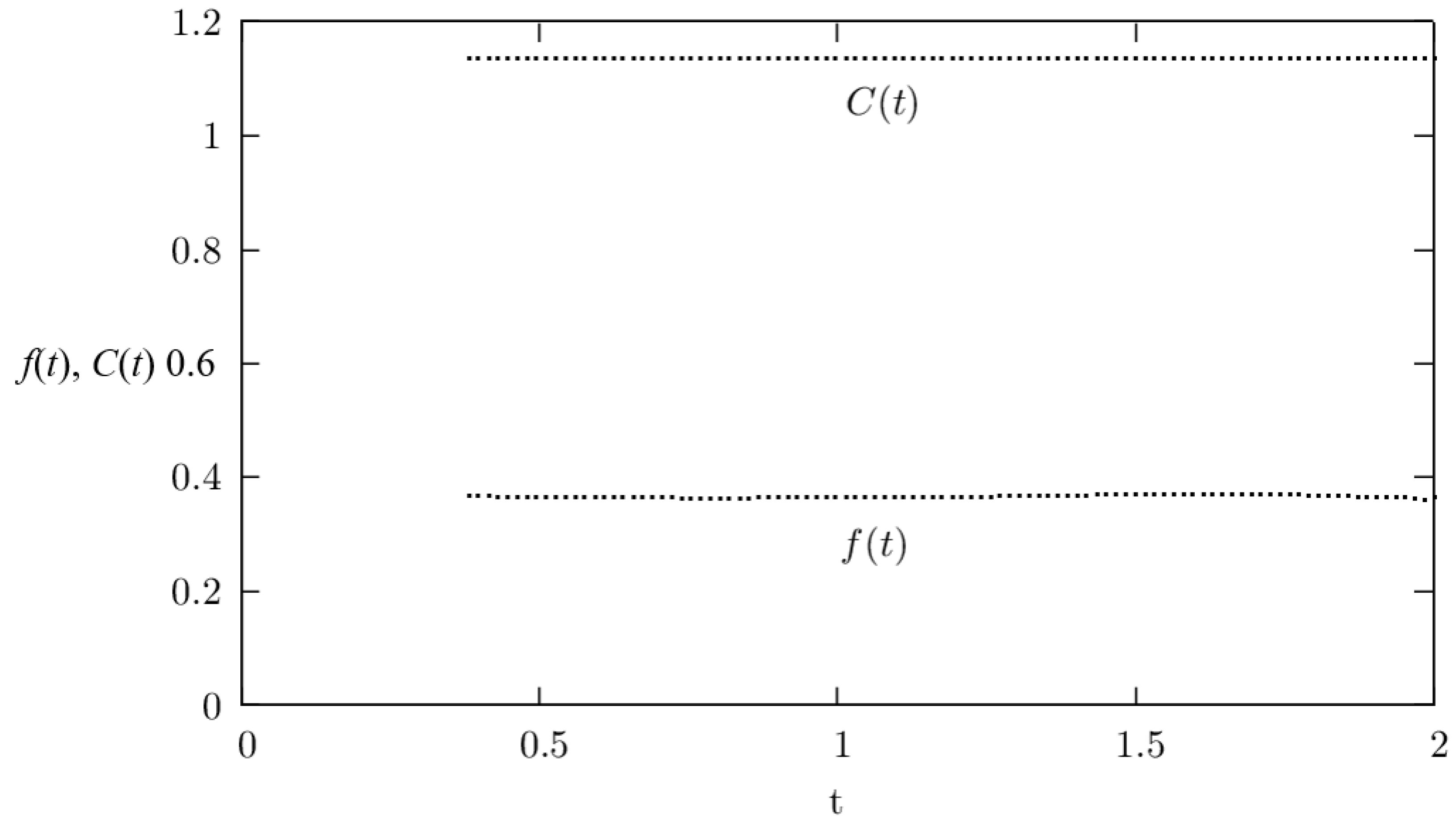
Example 5.

If $T=1$, $\mu =2$, $\gamma =1$ then $p\approx 0.661$, $t_e\approx 0.381$, and $C\left(t\right)\approx 1.485$. The density of the optimal arrival time at the interval $[t_e,T]$ is presented on Figure 2. In the figure, the function $f\left(t\right)$ decreases in the interval $[0.381,1]$.

6. N Players

The same approach can be used when considering a service system with more than 3 players. Suppose that in the queueing system an arrival strategy $F\left(t\right)$ of the form (1) is used, and the $\left(N\right)$-th player is looking for a strategy that gives the best response. In this case, the found best answer must coincide with the strategy $F\left(t\right)$. Due to symmetry, it will be the equilibrium in the game.

By the state of the system at an instant t, we mean the set $(k,s,i)$, where k is the number of claims entered into the system, i is the number of claims in the orbit, and the parameter s, which means for $s=0$ the server free, and with $s=1$ the server is busy at instant t. We denote by $W_i^j\left(t\right)$ the average time until the server seeks for a claim in orbit at the time t provided the system has not yet received j customers and there are i customers in the orbit. Our purpose is to find the average sojourn time of the $\left(N\right)$-th customer when they enter the system at the instant t. For $t=0$, we obtain:

$$\begin{array}{cc}\hfill C\left(0\right)& ={(1-p)}^{N-1}\frac{1}{\mu }+{\displaystyle \sum _{i=1}^{N-1}}{p}^i{(1-p)}^{N-1-i}\left(\frac{1}{\mu }+W_i^{N-1-i}\left(0\right))\right)\hfill \\ \hfill & =\frac{1}{\mu }+{\displaystyle \sum _{i=1}^{N-1}}{p}^i{(1-p)}^{N-1-i}{W}_i^{N-1-i}\left(0\right).\hfill \end{array}$$

For $0<t<t_e$, the average sojourn time of the $\left(N\right)$-th customer satisfies:

$$\begin{array}{cc}\hfill C\left(t\right)& ={(1-p)}^{N-1}\frac{1}{\mu }+{\displaystyle \sum _{i=1}^{N-1}}{p}^i{(1-p)}^{N-1-i}\left(\frac{1}{\mu }+W_i^{N-1-i}\left(t\right))\right)\hfill \\ \hfill & =\frac{1}{\mu }+{\displaystyle \sum _{i=1}^{N-1}}{p}^i{(1-p)}^{N-1-i}{W}_i^{N-1-i}\left(t\right).\hfill \end{array}$$

Finally, for $t\ge t_e$, the average sojourn time of the $\left(N\right)$-th customer equals:

$$\begin{array}{cc}\hfill & C\left(t\right)=P\left(\mathrm{idle\; server}\right)\frac{1}{\mu }+\hfill \\ \hfill & {\displaystyle \sum _{k=1}^{N-1}}{\displaystyle \sum _{i=0}^{k-1}}P(\mathrm{busy\; server},k\mathrm{arrived\; customers},i\mathrm{orbital\; customers})(W_i^{N-1-k}\left(t\right)+\frac{1}{\mu }).\hfill \end{array}$$

It gives:

$$C\left(t\right)={\displaystyle \sum _{k=1}^{N-1}}{\displaystyle \sum _{i=0}^{k-1}}\left(p_{k,0,i}\left(t\right)\frac{1}{\mu }+p_{k,1,i}\left(t\right)(W_i^{N-1-k}\left(t\right)+\frac{1}{\mu })\right),$$

implying, after some algebra, the following expression:

$$C\left(t\right)=\frac{1}{\mu }+{\displaystyle \sum _{k=1}^{N-1}}{\displaystyle \sum _{i=0}^{k-1}}{p}_{k,1,i}\left(t\right)W_i^{N-1-k}\left(t\right).$$

(17)

In this expression $p_{k,s,i}\left(t\right)$ denotes the state probability at the instant t, which satisfy the following Kolmogorov backward equations:

$$\begin{array}{ccc}\hfill p_{k,1,i}^{\prime }\left(t\right)=& -& (\mu +{\lambda }_k\left(t\right))p_{k,1,i}\left(t\right)+{\lambda }_{k-1}\left(t\right)p_{k-1,1,i-1}\left(t\right)\hfill \\ & +& {\lambda }_{k-1}\left(t\right)p_{k-1,0,i}\left(t\right)+\gamma p_{k,0,i+1}\left(t\right),\hfill \\ \\ \hfill p_{k,0,i}^{\prime }\left(t\right)=& -& (\gamma +{\lambda }_k\left(t\right))p_{k,0,i}\left(t\right)+\mu p_{k,1,i}\left(t\right);\hfill \\ \hfill k=& & 1,2,\dots ,N-2;i=0,\dots ,k-1.\hfill \end{array}$$

We note that in this case,

$${\lambda }_k\left(t\right)=(N-1-k)\frac{f\left(t\right)}{1-F\left(t\right)},k=1,\dots ,N-2,$$

is the arrival rate, provided there are k customers in the system at the instant t.

Then we find the expression for $W_i^j\left(t\right)$, the average waiting time a customer spends in the orbit, starting with instant t, until they occupy the server. Then, substituting $W_i^j\left(t\right)$ in (17), we proceed as above to find the optimal strategy for the $\left(N\right)$-th player. To do this, we require that the following conditions:

$$C\left(0\right)=C\left(t_e\right)=C\left(t\right)=C^{*},t\in [t_e,T],$$

are satisfied. Finally, these conditions allow, in general, one to find the optimal strategy $F\left(t\right)$ along the same steps we described above for particular cases with 2 and 3 players.

7. Conclusions

We consider a single-server retrial queueing system in which the service of customers is handled in a strategic manner, i.e., unlike the conventional retrial queues, the customers are generated by players who choose the time to occupy the server. An equilibrium is sought in such a system when applications are distributed in such a way that the average service time is minimal. An equilibrium is sought in the class of mixed strategies, when players choose the login time randomly. It is shown that the optimal strategy is such that a player enters the system with a non-zero probability at the initial moment of time, otherwise, it takes a random pause, and then a distribution density is used, satisfying a system of the differential equations. This setting is described in detail for the case of two and three players and illustrated by a few numerical examples. Moreover the model for an arbitrary number of players is formulated. This scenario is assumed to be considered in detail in a future work.

References

- Falin, G.I.; Templeton, J.G.D. Retrial Queues; Chapman & Hall: London, UK, 1997. [Google Scholar]
- Artalejo, J.R.; Gomez-Corral, A. Retrial Queueing Systems: A Computational Approach; Springer: Berlin/Heidelberg, Germany, 2008. [Google Scholar]
- Kim, J.; Kim, B. A survey of retrial queueing systems. Ann. Oper. Res. 2016, 247, 3–36. [Google Scholar] [CrossRef]
- Altman, E.; Borovkov, A.A. On the stability of retrial queues. Queueing Syst. 1997, 26, 343–363. [Google Scholar] [CrossRef]
- Morozov, E. A multiserver retrial queue: Regenerative stability analysis. Queueing Syst. 2007, 56, 157–168. [Google Scholar] [CrossRef]
- Morozov, E.; Phung-Duc, T. Stability analysis of a multiclass retrial system with classical retrial policy. Perform. Eval. 2017, 112, 15–26. [Google Scholar] [CrossRef]
- Morozov, E.; Steyaert, B. Stability Analysis of Regenerative Queueing Models; Springer: Berlin/Heidelberg, Germany, 2021. [Google Scholar] [CrossRef]
- Fayolle, G. A simple telephone exchange with delayed feedback. In Teletraffic Analysis and Computer Performance Evaluation; Boxma, O.J., Cohen, J.W., Tijms, H.C., Eds.; Elsevier: Amsterdam, The Netherlands, 1986; Volume 7, pp. 245–253. [Google Scholar]
- Choi, B.D.; Rhee, K.H.; Park, K.K. The M/G/1 retrial queue with retrial rate control policy. In Probability in the Engineering and Informational Sciences; Cambridge University Press: Cambridge, UK, 1993; Volume 7, pp. 29–46. [Google Scholar]
- Avrachenkov, K.; Morozov, E.; Steyaert, B. Sufficient stability conditions for multi-class constant retrial rate systems. Queueing Syst. 2016, 82, 149–171. [Google Scholar] [CrossRef] [Green Version]
- Morozov, E.; Zhukova, K. The Overflow Probability Asymptotics in a Single-Class Retrial System with General Retrieve Time. In Proceedings of the International Conference on Distributed Computer and Communication Networks, Moscow, Russia, 20–24 September 2021; DCCN 2021, LNCS 13144. Vishnevskiy, V.M., Samouylov, K.E., Kozyrev, D.V., Eds.; Springer: Cham, Switzerland, 2021; pp. 55–66. [Google Scholar]
- Dimitriou, I. A queueing system for modeling cooperative wireless networks with coupled relay nodes and synchronized packet arrivals. Perform. Eval. 2017, 114, 16–31. [Google Scholar] [CrossRef]
- Pappas, N.; Kountouris, M.; Ephremides, A.; Traganitis, A. Relay-assisted multiple access with full-duplex multi-packet reception. IEEE Trans. Wirel. Commun. 2015, 14, 3544–3558. [Google Scholar] [CrossRef] [Green Version]
- Morozov, E.; Morozova, T. On the stationary remaining service time in the queuieng systems. CEUR Workshop Proc. 2020, 2792, 140–149. [Google Scholar]
- Glazer, A.; Hassin, R. ?/M/1: On the equilibrium distribution of customer arrivals. Eur. J. Oper. Res. 1983, 13, 146–150. [Google Scholar] [CrossRef]
- Glazer, A.; Hassin, R. Equilibrium arrivals in queues with bulk service at scheduled times. Transp. Sci. 1987, 21, 273–278. [Google Scholar] [CrossRef]
- Altman, E.; Shimkin, N. Individually optimal dynamic routing in a processor sharing system. Oper. Res. 1998, 46, 776–784. [Google Scholar] [CrossRef] [Green Version]
- Mazalov, V.V.; Chuiko, J.V. Nash equilibrium in the optimal arrival time problem. Comput. Technol. 2006, 11, 60–71. [Google Scholar]
- Haviv, M.; Kella, O.; Kerner, Y. Equilibrium strategies in queues based on time or index of arrival. Prob. Eng. Inform. Sci. 2010, 24, 13–25. [Google Scholar] [CrossRef] [Green Version]
- Hassin, R.; Kleiner, Y. Equilibrium and optimal arrival patterns to a server with opening and closing times. IIE Trans. 2011, 43, 164–175. [Google Scholar] [CrossRef]
- Jane, R.; Juneja, S.; Shimkin, N. The concert queueing game: To wait or to be late. Discret. Event Dyn. Syst. 2011, 21, 103–138. [Google Scholar] [CrossRef]
- Haviv, M. When to arrive at a queue with tardiness costs. Perform. Eval. 2013, 70, 387–399. [Google Scholar] [CrossRef]
- Ravner, L.; Haviv, M. Strategic timing of arrivals to a finite queue multi-server loss system. Queueing Syst. 2015, 81, 71–96. [Google Scholar]
- Mazalov, V.; Chirkova, J. Networking Games. Network Forming Games and Games on Networks; Academic Press: Cambridge, MA, USA, 2019; 322p. [Google Scholar]
- Haviv, M.; Ravner, L. A survey of queueing systems with strategic timing of arrivals. Queueing Syst. 2021, 99, 163–198. [Google Scholar] [CrossRef]
- Boon, M.A.A. A polling model with reneging at polling instants. Ann. Oper. Res. 2012, 198, 5–23. [Google Scholar] [CrossRef] [Green Version]
Figure 1.
The equilibrium density and cost for .
Figure 2.
Equilibrium density and cost for .
Publisher’s Note: MDPI stays neutral with regard to jurisdictional claims in published maps and institutional affiliations. |
© 2022 by the authors. Licensee MDPI, Basel, Switzerland. This article is an open access article distributed under the terms and conditions of the Creative Commons Attribution (CC BY) license (https://creativecommons.org/licenses/by/4.0/).
Share and Cite
MDPI and ACS Style
Chirkova, J.; Mazalov, V.; Morozov, E. Equilibrium in a Queueing System with Retrials. Mathematics 2022, 10, 428. https://0-doi-org.brum.beds.ac.uk/10.3390/math10030428
AMA Style
Chirkova J, Mazalov V, Morozov E. Equilibrium in a Queueing System with Retrials. Mathematics. 2022; 10(3):428. https://0-doi-org.brum.beds.ac.uk/10.3390/math10030428
Chicago/Turabian StyleChirkova, Julia, Vladimir Mazalov, and Evsey Morozov. 2022. "Equilibrium in a Queueing System with Retrials" Mathematics 10, no. 3: 428. https://0-doi-org.brum.beds.ac.uk/10.3390/math10030428
Note that from the first issue of 2016, this journal uses article numbers instead of page numbers. See further details here.