
Do Commodities React More to Time-Varying Rare Disaster Risk? A Comparison of Commodity and Financial Assets

1
Department of Finance, School of Economics, Jinan University, Guangzhou 510632, China
2
Southern China Institute of Finance, Jinan University, Guangzhou 510632, China
3
Research & Development Center, Agricultural Bank of China, Guangzhou 511408, China
*
Author to whom correspondence should be addressed.
Mathematics 2022, 10(3), 445; https://0-doi-org.brum.beds.ac.uk/10.3390/math10030445
Submission received: 27 December 2021
/
Revised: 26 January 2022
/
Accepted: 28 January 2022
/
Published: 29 January 2022
(This article belongs to the Special Issue Mathematical and Statistical Methods Applications in Finance)
Abstract
:Using a rare disaster risk database from almost the last one hundred years, we examine the differences in the reaction of asset prices to rare disaster risk between commodity and financial assets. We first employ time-varying parameter VAR (TVP-VAR) models to investigate the role of rare disaster risk in the price dynamics of major asset markets. The results indicate that disaster risk generally has a more intense and persistent impact on crude oil and stock markets when compared to gold and bond markets. However, the role of rare disaster risk differs substantially between commodity and financial assets, as well as between the short and long term. Moreover, when using a nonparametric causality-in-quantiles method to detect causal relationships, we provide evidence of the nonlinear causality effect of rare disaster risks on asset volatilities, and not their returns, except for crude oil. In addition, we demonstrate that augmenting a diversified portfolio of stock or bonds with gold can significantly increase its risk-adjusted performance. The findings have important implications for investors as well as policymakers.
1. Introduction
Rare disaster risks, such as economic depressions or international conflicts and wars, constitute one of the main determinants of asset risk premium [1]. The probability of time-varying rare disasters might provide explanations for equity premium and high-volatility puzzles, and risk-free rate puzzles, as well as asset predictability [2], which is of great importance in asset allocation and risk management. Therefore, more efforts have recently been made to explore the effects of rare disaster risk on various financial assets in the theoretical and empirical literature.
Since Rietz proposes a theoretical discussion on the role of a market crash in explaining the equity risk premium puzzle [1], the theoretical modeling of the impact of rare disaster risk on asset price dynamics has often been discussed for equity markets, such as the equity premium puzzle [3,4], excess return predictability [3,4,5,6], and excess equity volatility [4,7], etc. For example, Barro [3] shows that it is possible to account for the high-risk premium on stock markets across the globe when using Rietz’s proposed model that incorporates the probability of rare disaster risk. Moreover, some studies have attempted to model the impact of rare disaster risk on other assets, including bonds [4,8], commodities [9], and exchange rates [10], among others.
Motivated by the theoretical pricing models on rare disaster risk, a number of empirical studies also seek to examine the relationship between rare disaster risk and asset prices. There is growing evidence, indicating that rare disaster risk has a significant impact on asset price dynamics, such as the excess returns and volatility in financial markets [6,11,12], the dynamics of commodity markets [13,14], and the dynamics of exchange markets [15,16]. In particular, due to the outbreak of the COVID-19 pandemic (epidemics of disease constitute one specific form of rare disasters [3]), some recent studies attempt to empirically investigate the response of asset markets to it, suggesting that the COVID-19 pandemic has a significant impact on the dynamics of asset prices [17,18,19].
Although previous work has documented a close link between rare disaster risk and asset prices, the focus is on the impact of rare disaster risk on asset prices, rather than the dynamic nature of their relationship. In addition, the existing literature has provided evidence that rare disaster risk is characterized by left-tail realization and high skewness [7,20]. Motivated by previous work in the literature, we are particularly interested in the possible nonlinear relationship between rare disaster risk and asset prices. Furthermore, to the best of our knowledge, there is no study by which assets’ price fluctuations are more closely related (or isolated) to the shocks of rare disasters, nor have any assessed the differences in the role of rare disaster risks in the fluctuations across different assets. Our empirical analysis complements the literature as we address the similarities as well as the differences of the responses of asset prices to rare disaster risks across a group of major commodity and financial assets, using a database collected over nearly a hundred years.
In this paper, we aim to investigate the impact of time-varying rare disaster risk on the price dynamics of major commodity and financial assets from 1918–2015. We are more interested in comparing the responses of prices to rare disaster risks across different assets. First, we construct the crisis severity index as a proxy for time-varying rare disaster risk by applying the approach proposed by Berkman et al. [6]. Next, we investigate the role of rare disaster risk in the price dynamics of major asset markets. Moreover, the possibly nonlinear causal effects of rare disaster risk on asset prices (i.e., returns and volatility) are examined based on a nonparametric causality-in-quantiles method. We further compare the differences in the effects of rare disaster risks between commodity and financial assets.
The paper contributes to the literature in the following ways. First, our paper adds to the literature by comparing the role of rare disaster risk in the fluctuations across asset markets. Different from previous studies, we are particularly interested in the differences in the effects of rare disaster risk between commodity and financial assets. We attempt to not only quantify and compare the differences in the effects of rare disaster risk on asset price dynamics, but also to address the similarities and differences of nonlinear causality between rare disaster risk and asset prices at different quantiles. Second, our paper adopts a novel nonparametric causality-in-quantiles method developed by Balcilar et al. [21] to detect possibly nonlinear causality in rare disasters on asset prices, relaxing the restriction of normal distribution in the traditional models. Since rare disaster risk is characterized by the left-tail realization [7,20], this method is advantageous in that it enables us to investigate higher-order causality in quantiles, such as causality in the second order (i.e., causality-in-variance) when compared to the traditional mean-based linear Granger causality test. Third, we use historical data collected over nearly a hundred years of potential international rare disaster crisis, which allows for subsuming a variety of crisis events to uncover the long-term dynamic nature, as well as avoiding the small sample problem in parameter calibration in theoretical models of rare disaster risk. Based on the ICB data, we construct a crisis severity index by aggregating a set of crisis indicators to measure rare disaster risks, which enables us to capture different aspects of the severity of the crises. Previous work typically focuses on a few economic cycles or individual-specific disasters, such as World War I, World War II, the global financial crisis in 2008, or the recent COVID-19 pandemic. The use of long-term and diverse rare disaster data is vital not only for an examination of the robustness and mitigation of data snooping biases, but also to control the misspecification due to nonlinearity.
2. Literature Review
Our paper is related to several strands of literatures on the links between rare disaster risk and asset prices. One strand of theoretical literature is motivated by rare disaster risk and its implication for asset pricing puzzles of stocks. Within the Arrow–Debreu asset pricing model, Rietz [1] first proposes that a market crash could be a way to explain the equity risk premium puzzle. By introducing time-varying rare disaster probability, Barro [3] extends Rietz’s model to calibrate disaster probabilities from major events in the twentieth century, such as World War I, World War II, and the Great Depression. In addition to resolving the puzzle of the high equity premium, the model established by Barro [3] sheds light on other financial puzzles, including low risk-free rate and volatile stock returns. Wachter [7] shows that high equity volatility and excess return predictability can be attributed to the time-varying probability of consumption disasters. When incorporating time-varying disaster intensity into the Rietz–Barro hypothesis, Gabaix [4] extends the time-varying rare disaster framework to understand different asset pricing puzzles. Gourio [22] introduces rare economic disaster risk into the real business cycle model, in which a higher probability of disaster leads to a decline in investment and output, and thus lower stock prices, as well as interest rates. When taking countries’ heterogeneous exposures to rare disaster risk into consideration, Gourio et al. [23] propose a theoretical model and the mechanism of how time-varying risks and heterogeneous exposures lead to worldwide recessions, drops in stock prices, interest rates, and negative returns on arbitrage trades. Moreover, Tsai and Wachter [24] incorporate rare booms and disasters into a multi-sector endowment economy, which accounts for higher expected returns of value stocks, with lower risk than that of growth stocks.
In addition to the stock market, the relationship between rare disaster risk and other assets has recently attracted renewed interest. For example, when examining the expected rate of return on gold within a Lucas-tree model that incorporates rare disasters related to consumption, Barro and Misra [25] show that gold does not deliver high average real returns during macroeconomic disasters. Barro and Liao [26] derive a new option-pricing method to analyze out-of-the-money options when rare disasters become the dominant force, allowing the impact of time-varying disaster risk to be taken into consideration when it comes to options pricing. Seo and Watcher [8] also construct an alternative and more general approach to modeling rare disaster risk to reconcile option prices with stochastic disasters, thus resolving the fact that the average implied volatility of equity options exceeds realized volatility. In terms of the relationship between rare disasters and exchange rates, Farhi and Gabaix [10] propose a new disaster-based tractable model for exchange rates, in which the probability of global disasters, as well as each country’s exposure to these events, are time-varying. This framework accounts for a series of major classic puzzles in exchange rates and the links between currency options, exchange rates, and interest rates. However, previous theoretical studies on the modeling of rare disasters in the literature are restricted to parameter estimation. The calibration and output of rare disaster models might be sensitive to the probability and distribution of rare disasters. For example, regarding worldwide political rare disasters, such as the World War I, the World War II, and the Cold War over the past century, if rare economic crises and regional territories are taken into consideration, the probability of rare disasters would differ greatly in the long run. In addition, from the perspective of mechanism, Skoufias [27] provides a review of the overall nature of economic crises and natural disasters, and then summarizes the mechanisms of how they affect household welfare, economic development, and thus asset prices.
Given the overwhelming arguments on the theoretical linkage between rare disaster risk and asset prices, an important question is to empirically examine to what extent the fluctuations of asset prices are related to rare disaster risk. In some recent empirical studies, for example, Berkman et al. [6] attempt to examine time-varying rare disaster risk and stock returns by constructing a crisis severity index based on international political crises from 1918–2006 from the ICB (International Crisis Behavior, hereafter) database. Following Berkman’s method, Huang et al. [28] show that global political crises increase the market perceived uncertainty, and thus raise the cost of external financing. Subsequently, using global political instability from the ICB database as a proxy for rare disaster risk, Berkman et al. [11] find that rare disaster risk is positively related to expected excess stock market returns, as well as valuation ratios (E/P and D/P). MengYun et al. [29] quantify the impact of terrorism and political instability on the equity market and find that these non-economic factors have a significant negative impact on the firm equity premium in Pakistan. Gkillas et al. [30] apply a quantile dependence approach to investigate the quantile dependencies between equity price discontinuities (jumps) and time-varying rare disaster risks, providing evidence of an asymmetric relationship between jumps and rare disaster risks. Meanwhile, a few recent studies further explore the role of rare disaster risks on other financial asset dynamics. For example, when examining the impact of rare disaster risks on bond market dynamics, Gupta et al. [31] demonstrate that rare disaster risks affect only the volatility of government bonds, not their returns. Similarly, using the HAR-RV model to determine the role of rare disaster risks (measured by ENSO cycle), van Eyden et al. [32] demonstrate a positive and statistically significant effect of the ENSO cycle on the volatility of Treasury securities of the US.
Moreover, some empirical studies have also tried to link the rare disaster risk to the dynamics of commodity assets. For example, Demirer et al. [13] provide a novel perspective on the ability of rare disaster risks to predict the oil market, showing that rare disaster-risks strongly affect oil returns and volatility, along with the evidence of stronger predictability observed at lower quantiles of the respective conditional distributions. Demirer et al. [33] investigate the effect of rare disaster risks (i.e., the El Niño-Southern Oscillation (ENSO)) on crude oil prices, via a nonparametric causality-in-quantile framework, and show that the ENSO cycle not only predicts real WTI oil returns, but also the volatility.
In particular, the outbreak of the current COVID-19 pandemic has substantially shifted the global economy, as well as the financial markets. To understand the impact of the current COVID-19, Adekoya and Oliyide [34] attempt to explore the role of the pandemic in the connectedness among the globally traded commodity and financial markets, proving that the pandemic is largely responsible for the risk transmission across various markets. Similarly, using a sample of the G20 countries, Bissoondoyal-Bheenick et al. [35] examine the impact of COVID-19 on stock return and volatility connectedness, and whether the connectedness behaves differently for countries with SARS 2003 experience. They show that connectedness increases across the phases of the COVID-19 pandemic. However, the degree of connectedness is significantly lower in countries with SARS 2003 death experience. Moreover, Mensi et al. [36] examine the impacts of COVID-19 on the asymmetric multifractality of commodity prices based on upward (downward) trends, and document that gold and oil markets have become more inefficient during the pandemic outbreak compared to the pre-COVID-19 period. When studying the impacts of the COVID-19 pandemic, Harjoto et al. [37] show that equity markets react negatively to the pandemic, while the impacts differ greatly between emerging and developed markets.
3. Econometric Methodology
3.1. Time-Varying Parameter VAR Model
We start by adopting the time-varying parameter VAR (TVP-VAR) model developed by Primiceri [38] to explore the role of rare disaster risk in the fluctuations of asset markets. The TVP-VAR model with stochastic volatility is often used to capture the possible heteroscedasticity of the shocks, as well as the simultaneous relations among the variables of the system. Furthermore, by allowing the parameters to change over time, it leaves it up to the data to determine whether the time variation of the linear structure results from changes in the size of the shocks or from changes in the response. Therefore, this model has been widely used to capture the possible features of the nonlinearities or time-varying effects of structural shocks [39,40,41].
The TVP-VAR model is derived from the basic VAR model, which is defined as follows:
where is an vector of observed endogenous variables in the system; is an vector of time-varying coefficients that multiply constant terms; , are matrices of time-varying coefficients; and are heteroscedastic unobservable shocks with variance-covariance matrix . Without loss of generality, the triangular reduction of is defined as follows:
where is the lower triangular matrix:
and is the diagonal matrix:
Thus, the model can be modified as follows:
Stacking all the R.H.S. coefficients in a vector of , Equation (5) can be rewritten as the following specification:
where the symbol denotes the Kronecker product.
In order to model the process for the time-varying parameters in Equation (6), we follow Primiceri [38] to assume that the parameters follow a random walk process, and all the innovations are jointly normally distributed as follows:
where ), and for ; and refers to the vector of the diagonal elements of the matrix with ,. This assumption of random walk presents the advantages of focusing on permanent shifts and reducing the number of parameters in the estimation procedure, since the sample period is just a finite period of time, and not forever. The shocks to the innovations of time-varying parameters are assumed to be uncorrelated among the parameters . Furthermore, are assumed to all be diagonal matrices. The drifting coefficients and parameters are modeled to fully capture possible changes of the VAR structure over time. The dynamic specification is adequate to permit the parameters to vary, even if the shocks in the processes driving the time-varying parameters are uncorrelated.
In the paper, we adopt a Bayesian approach using the MCMC method for a precise and efficient estimation of the TVP regression model, which is widely used in the literature, and has been proven to produce good results [42,43]. In the Bayesian procedure, it allows one to estimate more general specifications for a non-trivial number of equations (For specification and estimation of a time-varying VAR model, see Primiceri [38]. And for specification and estimation of a time-varying SUR model, see Chib and Greenberg [44]). The prior distributions are assigned to the hyperparameters in the model and then are combined with the information contained in the data (via the form of likelihood function). Together with a set of initial conditions, the joint posterior distribution of the parameters can be estimated through Bayesian methods. The Bayesian approach allows us to produce the sample drawn from a posterior distribution of parameters, including the unobserved latent variables suggested by Chib [45]. When using time-varying parameters in the model as latent variables, the model can be formed as a state-space specification. Since the model has the forms with a non-linear and non-Gaussian state space, we need to find some ways of sampling. Therefore, we follow the method of the mixture sampler which has been widely used in the financial and macroeconomics literature [38,46,47]. It consists of transforming a nonlinear and non-Gaussian state space form into a linear and approximately Gaussian one, which allows the use of standard simulation smoothers. Following these procedures, we can obtain the estimates of both time-varying parameters and variance-covariance matrix in the VAR Model.
3.2. Nonparametric Causality-in-Quantiles Method
Beyond exploring the role of rare disaster risk in the asset market fluctuations, we further employ a nonparametric causality-in-quantiles method to investigate their possibly nonlinear causal relationship between rare disaster risk and asset prices. This novel methodology for the detection of nonlinear causality has been proposed by Balcilar et al. [21], which is based on the frameworks of Nishiyama et al. [42] and Jeong et al. [48]. In recent literature, the approach has been widely used to examine the causal effect on asset price dynamics due to the advantage of the framework for combining quantile regression with nonparametric estimation [21,34,49].
In the model, we denote asset returns as and rare disaster risk as . We then follow Jeong et al. [48] to define the quantile-based causality as follows: does not cause in the -th quantile under the condition of if
and causes in the -th quantile under the condition of if
where refers to -th quantile of at time t and .
Based on the Equations of (8) and (9), we further test the hypothesis of causality-in-quantiles as follows:
where , , and . Here refers to the conditional distribution of under . denotes the possibility. Therefore, is not the -th quantile cause of with respect to the lag vector of if the null hypothesis is not rejected.
Based on the null hypothesis in Equation (8), the regression error is defined as (12). The null hypothesis in Equation (10) is true if and only if Equation (12) or equivalently holds, where is an indicator function:
Jeong et al. [48] utilize a distance measure , where is the regression error and refers to the marginal density function of .
According to Jeong et al. [48], the test statistic function J is specified with a feasible kernel-based analogue :
where denotes the kernel function with a sample size T, a bandwidth h, and a lag order p. And is the estimated unknown regression error based on the equation as follows:
Employing the nonparametric kernel method, , the estimation of -th conditional quantile of given is specified as
We utilize the Nadarya–Watson kernel estimator to estimate as:
with is the kernel function and is the bandwidth.
This methodology also allows us to investigate higher order causality in quantile, such as quantile causality in the second order, which is an attractive feature compared to the traditional mean-based linear Granger causality test. Within this model, for example, we can test the causality between rare disaster risk and the volatility of asset returns. Balcilar et al. [21] extend the framework of Jeong et al. [48] and develop a higher order causality-in-quantiles method based on the approaches in Nishiyama et al. [42]. In order to illustrate the causality in higher-order moments, consider the following process for :
where is a white noise process, and are unknown functions that satisfy certain conditions for stationarity. We re-formulate Equation (15) into a null and alternative hypothesis for causality in variance as follows:
To obtain a feasible test statistic for testing the null hypothesis in Equation (15), we replace in Equations (13)–(16) with . For higher-order causality, we interpret the causality using the following model:
Therefore, the hypotheses are re-organized as follows in -th order:
Compared with Equations (10) and (11), the entire framework is re-established to test whether Granger causes in θth quantile up to the kth moment via Equation (21), and to formulate the test statistic in Equation (16) for k = 1, 2, … K. However, due to the mutually correlated statistics proposed by Nishiyama et al. [42], it is difficult to integrate different test statistics for each into one statistic for the joint null hypothesis in Equation (21). Balcilar et al. [21] resolve this problem via proposing a modified sequential testing method based on Nishiyama et al. [42]. The main steps are as follows. First, a nonparametric causality-in-quantile for the first moment is tested. If the null hypothesis of Equation (14) is rejected, it suggests that there is a strong indication of Granger quantile-causality in mean. In contrast to the classical mean-based linear Granger test, failing to reject the null hypothesis for the first order test does not necessarily lead to no causality in the second or higher moment. Thus, tests for k can be further constructed.
There are several important parameters in the models that need to be specified here: the bandwidth (h), the lag order (p), and the kernel function for and . First, the bandwidth (h) is selected according to the leave-one-out least squares cross-validation method for each quantile, and the lag order (p) is determined based on the Schwarz Information Criterion (SIC). Second, Gaussian-type kernels are employed for and in Equations (13) and (16), respectively.
4. Data and Preliminary Analysis
4.1. Measure of Rare Disaster Risk
To examine the relationship between rare disaster risk and asset prices, this paper involves two major types of annual data: crisis severity index as a proxy for time-varying rare disaster risk and price indices of a group of major asset classes including financial asset (i.e., stock and bond) and commodity (i.e., crude oil and gold) from 1918–2015 (Data on crisis index is only available for the period 1918–2015 in the ICB database. The sample period is therefore set as 1918–2015 in the paper).
In the paper, we use the occurrence of international political crises as our proxy for rare disaster risk. The crises data are obtained from the International Crisis Behavior (ICB) database (the database, known as the International Crisis Behavior (ICB) project, has been developed by the Center for International Development and Conflict Management since 1975. Detail explanation of the variables and extensive discussion of the system level data can be found at https://sites.duke.edu/icbdata/ (accessed on 16 October 2018)), in which 476 international crises and 1052 crisis actors are included from 1918 to 2015. We exclude five crises from the analysis, since the database does not specify an explicit end date. The resulting sample consists of 471 international political crises in the paper. The ICB database documents international crises from a variety of aspects. There are 81 crisis dimensions for every crisis, recording key information about the crisis, such as the gravity of value threatened, regional or security organization involvement, and so on. One of the attractive features of ICB database is its definition of crisis, which is in accordance with the concept of rare disaster risk. In contrast with natural events, international political crises are more likely to affect investor sentiment or risk preference. Moreover, according to the ICB database’s documentation, rather than simply defining a crisis with an actual attack or political action, a crisis is defined as a perceived change in the likelihood of a threat that can cause the beginning or end of an international political disaster with the following three characteristics: (1) a threat to more than one basic value, (2) a high likelihood of military hostilities involvement, and (3) an awareness of a finite time for response to the value threat. Therefore, this database loosens the restriction of a small sample problem, which allows us to have a wider perspective rather than merely focusing on the impact of World War I and World War II.
A large number of variables are contained in the ICB datasets related to different aspects of international political crisis. Following Berkman et al. [6], we use six indicators to characterize the severity dimensions of crises, including whether or not a crisis started with violence, violence used during the crisis, full-scale wars, gravity of value threat, protracted conflict, and major power (great power or superpower) involvement. Each of the six types above has a matching dummy variable that is assumed to be a value of one if a crisis is in that type, and zero otherwise. We follow Berkman et al. [6] to measure the crisis severity index (CSI) by aggregating the indicators of six severity dimensions of political crises, as follows:
where is the crisis severity index; N is the number of the specific crisis at time t, and the right-hand side of the equation includes six dummy variables: is “Violence break”, is “Grave threat”, is “Full-scale Wars”, is “Violence during Crisis”, is “Major power involved”, and stands for “Protracted conflict”. N indicates the number of the related types of events.
We construct a crisis severity index that summarizes the different aspects of crisis severity into one measure by aggregating the six variables above and adding one (being a specific type of crisis). We utilize the information of the duration date to capture the states of crises. The detail of the definition of dummy variables included in the discussion can be found in Table 1. The column of “Value” presents the code of the event, in which the dummy variable equals 1 when the code appears in the disaster table.
4.2. Data of Asset Prices
Our empirical analysis attempts to explore the effect of rare disaster risk on the prices of major asset classes. The dataset of asset classes in this paper consists of price indices of financial assets (i.e., the US stock (S&P500) and the US 10-year treasury bonds) and commodity (i.e., crude oil and gold) from 1918 to 2015. Annual data on stock price indices and bond indices are taken from Robert Shiller’s publication Irrational Exuberance (Shiller, Robert J. Irrational exuberance. Princeton university press, 2000. Online dataset: http://www.econ.yale.edu/~shiller/data.htm (accessed on 16 October 2018)). We collect annual oil prices in dollars from British Petroleum (The link of the annual oil prices can be found as follows: https://www.quandl.com/ (accessed on 16 October 2018)) and the historical gold prices in dollars from the National Mining Association (The link of the annual gold prices can be found as follows: https://nma.org/wp-content/uploads/2016/09/historic_gold_prices_1833_pres.pdf (accessed on 16 October 2018)). After acquiring all asset prices from 1918–2015, we use first logarithmic difference to obtain annual asset returns.
4.3. Preliminary Analysis
The annual number of international political crises and crisis severity index during the period of 1918–2015 according to the ICB database is shown in Figure 1, along with the result of summary statistics of crisis dimensions which consists of the crisis severity index in Table 2. The six dummy variables provide a picture of some detailed characteristics of international political crises over nearly a recent century in our sample. As shown in Table 2, among all the crises, 194 crises began with a violent break, 211 crises involved serious violence, and 83 crises were full-scale wars. There are 258 crises that involved threats of the most basic values at some time during the crisis, in which 66 crises were related to protracted conflicts, and major power was involved in 159 conflicts.
We take a first look at the difference and similarity of a variety of crisis variables and asset markets. Table 3 reports descriptive statistics of the crisis variables and four different assets in our sample. As shown in Table 3, there exists a significant variation in the returns across different assets. In general, the annual returns of the bond market are relatively stable in the sample period, followed by gold and stock markets, while the crude oil market is the most volatile, in which the annual returns range from −64.7 percent to 125.8 percent.
5. Empirical Results
5.1. Impact of Rare Disaster Risk on Asset Prices
In this section, we use basic VAR and TVP-VAR approaches to examine the responses of various asset markets to the shock of rare disaster risk, as well as to quantify the proportion of asset market volatility attributed to rare disaster risk. In this paper, we use MATLAB software to estimate the TVP-VAR model.
5.1.1. Variance Decomposition Results
We first employ a standard VAR model to quantify the contribution of rare disaster risk to the fluctuations in different asset markets. Before the VAR analysis, we need to examine the stationarity of the variables in the system. The result of the ADF test indicates that asset returns as well as rare disaster risk in the model are stationary. The variables included in the VAR model are as follows: rare disaster risk, stock returns, bond returns, oil returns, and gold returns. The lag length of the VAR is chosen based on the selection criteria of AIC and SIC, leading to an optimal lag length of 5. Table 4 reports the result of forecast errors variance decomposition (FEVD) in the asset volatility due to rare disaster risk at several selected forecast lengths.
As shown in Table 4, it is indicated that in the short-term, the fluctuation of crude oil market among different assets in the VAR system is the most related to rare disaster risk. For example, rare disaster risk explains about 3.23 percent of the variance of oil market returns at one-period ahead, while it accounts for less than 1 percent of the volatility of three other asset markets. For example, only about 0.36 percent and 0.39 percent of the variances of gold and stock returns can be explained by the shocks of rare disaster risk. On the other hand, in the long run, the impact of rare disaster risk accounts for a significant proportion of the variance of asset returns. Interestingly, we find that the fluctuation of the stock market is the most related to rare disaster risk long term, where rare disaster risk explains about 13.07 percent of stock market volatility. It is followed by the crude oil market, in which about 9.85 percent of the volatility can be attributable to rare disaster risk. In contrast, the proportions of the variance of gold and bond returns contributed by rare disaster risk are about 4.85 percent and 2.97 percent, respectively. The result supports the views of Berkman et al. [6] that the impact of disaster events generally resonates in major financial markets.
Combing the empirical evidence above, we find some interesting phenomena among these assets. First, rare disaster risk has greatly different impacts on the volatility of major asset markets at various time durations. Second, the result of the VAR analysis shows that the rare disaster risk has persistent and strong effects on the oil market volatility, both short and long term. Moreover, the volatility of the stock market responds much more strongly to the rare disaster risk long term rather than short term. However, compared to crude oil and stock markets, rare disaster risk has relatively less explanation power for gold and bond market volatilities. The finding, therefore, provides evidence that the gold and bond may serve as hedging or safe-haven assets during periods of financial turmoil or crises [31,50].
5.1.2. Time-Varying Impulse Response Analysis
In this subsection, we further employ the TVP-VAR model to examine the dynamic relationship between rare disaster risk and asset returns. Compared to the standard VAR approach, the TVP-VAR model enables us to capture the pattern of the time-varying effects of rare disaster risk. After checking the stability of the parameters in the VAR, we employ the method of Markov chain Monte Carlo (i.e., MCMC) in the context of a Bayesian inference to estimate the posterior of the parameters in this model. The MCMC algorithm has been widely used for the numerical estimation of the posterior of parameters in the literature. Regarding the time-varying parameters in our model as latent variables, we take advantage of the Bayesian sampling procedure to construct a state space specification. The estimation steps in detail can be found in Nakajima et al. [38].
Thus, following Nakajima et al. [38], we select the optimum lag length determined by the estimated marginal likelihood, and the result supports the optimal selection of a lag length of 2. For the initial state of the time-varying parameters, and . The priors for the -th diagonals of the covariance matrices are assumed to be: , , . We draw 10,000 samples after the initial 1000 samples are discarded to allow for convergence. The posterior estimates are presented in Table 5 and Figure 2, respectively.
We performed the tests for the convergence and efficiency for the estimates of the TVP-VAR model. Table 5 presents the posterior estimates for selected parameters of the TVP-VAR model, including the posterior means, standard deviations, 95% confidence intervals, Geweke convergence statistics, and inefficiency factors. As shown in the table, for all parameters, their Geweke convergence statistics are less than the critical value under the 5% significant level (i.e., the corresponding Z-score 1.96; the convergence diagnostic (CD) statistics of Geweke are basically a single-chain Z-test to compare means for the early and latter parts of the Markov chain. Thus, the critical value under the 5% significance level is 1.96), indicating that the null hypothesis of the convergence to the posterior distributions cannot be rejected. Moreover, the low inefficiency factors (as shown in the column of inefficiency in Table 5) confirm the inefficiency sampling for the posterior draws of parameters in the TVP-VAR model.
Figure 2 shows the sample autocorrelation function (top), the sample paths (middle) and the posterior densities (bottom) for selected parameters, respectively. After discarding the sample in the burn-in period, the path of the sample seems to be stable and the autocorrelation of the sample gradually decreases, indicating that our sampling method efficiently produces uncorrelated samples.
Furthermore, we estimate the responses of different asset returns from the variance–covariance matrix of the TVP-VAR model. Figure 3, Figure 4 and Figure 5 present plots of the evolution of the responses of asset markets to a 1 percent change in rare disaster risk over the last 98 years. Figure 3 represents the simultaneous response, and Figure 4 and Figure 5, the responses after 3 and 5 years. Taken together, these results reported in the figures indicate some important regularities among different asset markets.
First, gold asset, in general, is positively correlated with rare disaster risk, with some exceptions in the past decade. As shown in Figure 3, the contemporaneous response of gold market to rare disaster risk is strong and time-varying. In the short term, the positive impact of rare disaster risk on gold prices increased from 1960s–1970s, reaching its highest point in the early 1980s; then, it turned to decrease after that, which may be due to the worst recession since World War II. In the presence of the subprime mortgage crises since 2007, the response of gold prices turned out to be negative. This may be due to the fact that increasing investor’s negative sentiment outweighs the sentiment of risk aversion, and thus the emergence of gold monetization in the market. In addition, the impact of rare disaster risk on the gold market is stronger in the short term than in the long term. Overall, during the period of rare disaster risk, gold can be used as a safe asset to some extent, which is consistent with the result of the test of causality-in-quantiles in Section 4.2. This finding provides detailed evidence on how the changes in gold prices are sensitive to the main determinant of risk occurrence.
Second, similar to the response of gold asset to rare disaster risk, crude oil is also positively correlated with rare disaster risk, with some exceptions in the recent two decades. However, compared to the gold market, the crude oil market has a stronger response to the crisis shocks, while it converges more slowly. Interestingly, the response is remarkable during the energy crisis from the 1970s to the early 1980s. This may be attributed to the fact that “Superpower Involvement” and “Grave Threat” are the major components of the crisis severity index during these periods. In general, the crude oil market appears to respond much more strongly during the periods when a superpower is involved in both sides of the conflicts or when facing various threats. The findings confirm that the predictive power of rare disaster risk over oil market dynamics is statistically significant for both the conditional distributions of returns and volatility.
Third, rare disaster risk, in general, has a negative impact on the stock and bond markets, although the dynamic responses of these two financial assets behave quite differently. International political crises increase the uncertainty and instability regarding future economic activities worldwide, which thus significantly impacts the confidence of global investors in financial assets. The analysis provides insight into the effect of rare disaster shocks on different financial markets from a time-varying angle. In particular, the simultaneous negative responses to rare disaster risk for the two financial assets are high, suggesting that stocks as well as bonds are very sensitive to the type of risk. However, the short-term reaction of the stock market to rare disaster risk is higher than that of the bond market. This may be expected due to the difference of fundamental pricing between these two financial assets [51]. Stock prices are determined by both uncertain cash flows and the discount rate, while bond prices depend more on the discount rate. Rare disaster risk is closely related to the future information affecting uncertain cash flow. Thus, the difference between them may be reflected in the different reactions to rare disaster risks.
Fourth, as shown in Figure 4, the response of bond returns to the shock of disaster risk faded over the medium term. Moreover, the bond returns have converged faster than those of other assets in response to disaster risk shocks. Meanwhile, the effects of rare disaster risk to stock and oil returns are greater than gold and bond returns in the medium term. The impulse response has almost all converged in five years. This is expected, as the information on the uncertainty obtained from the rare disaster shocks has been transferred and been diversified by financial market investors, which results in a strong response of asset prices in the short term, and then the impact gradually disappears in the long term.
Overall, rare disaster risk exerts a more intense and persistent influence on crude oil and stock markets, when compared to gold and bond markets. This is not surprising, due to the fact that energy and stock markets can be shaken by profound political crisis changes, as well as the resulting friction and tension, or by episodes of major disasters. This result confirms that the finding of variance decomposition in the subsection above indicates that rare disaster risk accounts for a higher proportion of the volatility of oil and stock markets than bond and gold markets. Furthermore, it also verifies that the assets of gold and bond are favored by investors as hedge assets during crisis periods [31,50].
5.1.3. Impulse Response Analysis of Typical Episodes
In addition, we further investigate the impulse responses at a couple of specific dates of the sample, which is a complement to the time-varying impulse response analysis in the TVP-VAR model. The years (episodes) chosen for the comparison are 1950, 1981, 1992, and 2007. Due to the fact that the number of political crises reached their peak values in these years, they are somewhat representative of the typical economic conditions and the international political crisis background (The years with higher rare disaster risk appear to be more representative of the typical political crisis background when examining the impact of rare disaster risk on asset prices, which enables one to capture typical economic conditions. For example, during the period of post-World War II in 1950, the crisis severity index reached 81, in which 53% of the index is composed of the factor of “Superpower Involvement”. Similarly, in 1981 and 1992, more than 50% of the number of political crises are involved in the subset “Grave Threat”, including a territorial threat, a threat of grave damage, or a threat to existence. In 2007, since the U.S. experienced the subprime mortgage crisis which led to the most serious global recession since the Second World War, 96% of the crisis severity index has been calculated by the subset “Superpower Involvement”). Figure 6 reports the changes in the impulse response of asset markets to rare disaster risk shock in the four selected years in the sample. Clearly, the dynamic responses of different assets to the shocks of rare disasters behave quite differently. The empirical finding provides further support for the time-varying effect of rare disaster risk on different asset prices.
As shown in Figure 6, the responses to disaster risk shocks differ greatly across commodity and financial assets in the specific dates of the sample. Overall, the response of oil and stock returns converges more slowly than gold and bond returns. In 2007, the short-term response is negative, and the response intensity is greater than that of the other three disaster years. It can be explained that the outbreak of the financial crisis has a huge impact on the financial market, and the whole market is in a liquidity squeeze.
Although the responses to disaster risk shocks still fluctuate very slightly after the initial three or four periods for all assets in the sample years (except 1950), they gradually approach zero thereafter. For the case of 1950, the response of all the assets begins to converge until the sixth period, while for the other three selected years (i.e., 1981, 1992, and 2007), it generally converges after the third or fourth period. This may be due to the fact that the global economic activity was in the early stages of recovery after World War II, and asset markets may be slow to recover from the new crisis shocks. Although the impact of disaster risk on commodity assets is very mixed across different selected years, the responses of the commodities are consistent in both 1992 and 2007, which may be due to the increasing financialization of crude oil. Moreover, rare disaster risk has a greater impact on the oil and stock markets compared to the gold and bond markets; this is consistent with the empirical results of variance decomposition.
5.2. Causal Relationship between Rare Disaster Risk and Asset Prices
In the above section, we demonstrate the asymmetric role of rare disaster risk in the fluctuations across asset markets over time via using VAR approaches. Furthermore, we aim to investigate whether rare disaster risk has nonlinear causal effects on asset prices. Using the crisis severity index as a proxy for rare disaster risk, we employ a nonparametric causality-in-quantiles method to capture the possibility of the nonlinear causal relationship between rare disaster risk and asset prices, including asset returns, as well as volatility. We use R language programming to obtain the following empirical results.
Figure 7 presents the results of the causality-in-quantiles tests when we regress rare disaster risk against the returns, as well as the volatility of four assets, respectively. In addition, we report the detailed empirical results of each 5% quantile analysis based on the nonparametric causality-in-quantiles test in Table 6, along with the summarized results in Table 7. The mean and variance statistics for asset prices (including asset returns or volatility), reported in both Figure 7 and Table 6, are the standardized test statistics calculated on the basis of the causality-in-quantiles tests.
We first focus on the nonlinear causal effect of the time-varying rare disaster risk on asset prices. As shown in Figure 7, the causal relationship between rare disaster risk and asset returns is non-significant, except for crude oil. In general, there is no significant evidence of nonlinear causality between rare disaster risk and asset returns at different quantiles among three assets, including stock, bond, and gold. In particular, as reported in both Figure 7 and Table 6, the asset mean values of test statistics of the causality-in-quantiles tests for stocks and bonds are approximately zero as compared to commodities, indicating that disaster risk has a negligible impact on financial assets. In contrast, the result shows that the impact of disaster risk on crude oil returns is significant for quantile at about 0.35 to 0.45, while the causality-in-quantiles becomes non-significant for quantiles below about 0.35 as well as above 0.45. The findings indicate that there is a significant role of international political crises in the crude oil market, especially the impact of armed conflicts, which has been documented in the literature. For example, in earlier studies, Lieber [52] provides evidence of a surge in crude oil prices during the Gulf War, and Rigobon and Sack [53] and Leigh et al. [54] demonstrate that the increased risk of wars in Iraq led to crude oil price being much higher.
However, when turning the attention to the second order causal relationship (namely causality-in-variance), we find that rare disaster risk has a significant causal impact on the volatility of financial assets, with some exceptions in the extreme low or high quantiles of its conditional distribution. Figure 7a provides visual evidence of the hump-shaped pattern of the causality in variance across quantiles for the majority of the conditional distributions of stock market volatility, with the exception of extreme ends. In terms of the bond market, we find a very similar pattern of the causality in variance across quantiles. As shown in Figure 7, the causal impact is significant in the majority of cases around the median quantiles for the conditional distribution of bond returns, while not being significant for the quantiles below about 0.20 and above 0.80. The empirical findings indicate that the causality impact is not significant in either the upper or lower quantiles of the conditional distribution of financial asset volatility. This further supports the theory of market inefficiencies in the cases of extreme circumstances, which is consistent with the finding of Urquhart [55].
By comparison, in terms of commodity market volatility (i.e., crude oil and gold) in Figure 7c,d, the results of the causality-in-quantiles analysis indicate more differences than similarities between commodity and financial assets as far as the patterns of causal effects are concerned. In general, the result of the causality-in-variance provides evidence of a similar pattern of causal effects of rare disaster risk between these two commodity assets. Interestingly, the causal effects of rare disaster risk on the commodity market volatility are asymmetric, as they are significant for different quantiles except for the upper quantiles, i.e., with the causality only being insignificant in quantiles above about 0.85 for crude oil and above 0.75 for gold. In contrast, the causal effects are not significant at both extremely lower or higher quantiles for financial assets.
In addition, the result also indicates that rare disaster risk is more likely to affect the volatility rather than the returns of different assets. When the volatility is extremely low (i.e., the financial market is relatively calm), investors may rely more on fundamental factors, while other information would be subordinate. On the contrary, in the presence of high volatility, other types of rare disaster risk such as economic and financial crises might be the first concern for investors. Our findings above also demonstrate the role of international political crises (as a proxy for rare disaster risk) in the volatility of asset markets.
5.3. Implications for Portfolio Diversification
Investors often choose some safe assets to hedge market risks and benefit from the diversification in the presence of increasing market risk. The above empirical results show that the gold and bond prices are less affected by rare disaster risk, and, in general, that the disaster risk shock has a positive impact on gold, with a negative impact on bonds. Taken together, we thus choose gold as a safe asset to build portfolios, including gold–stock, gold–oil, and gold–bond. The optimal weights of the portfolios and hedging ratios are determined based on the results of the variance–covariance matrix derived from our TVP-VAR model. In the empirical work, the method proposed by Kroner and Ng [56] is often used to determine the optimal weights over time. For example, Jebabli et al. [43] adopt this approach to calculate the optimal weight and hedging ratio of oil–food portfolios.
The equation for calculating the weight of the portfolio is as follows:
Moreover:
Here, is the conditional volatility of an asset (stock/bond/oil/gold) at time t and represents the conditional covariance between asset 1 and asset 2 at time t, which are both obtained according to the result of the TVP-VAR model. The weight of stock/bond/oil in the portfolio is . Following Kroner and Sultan [57], we further calculate the hedge ratios with risk minimization for the portfolio as:
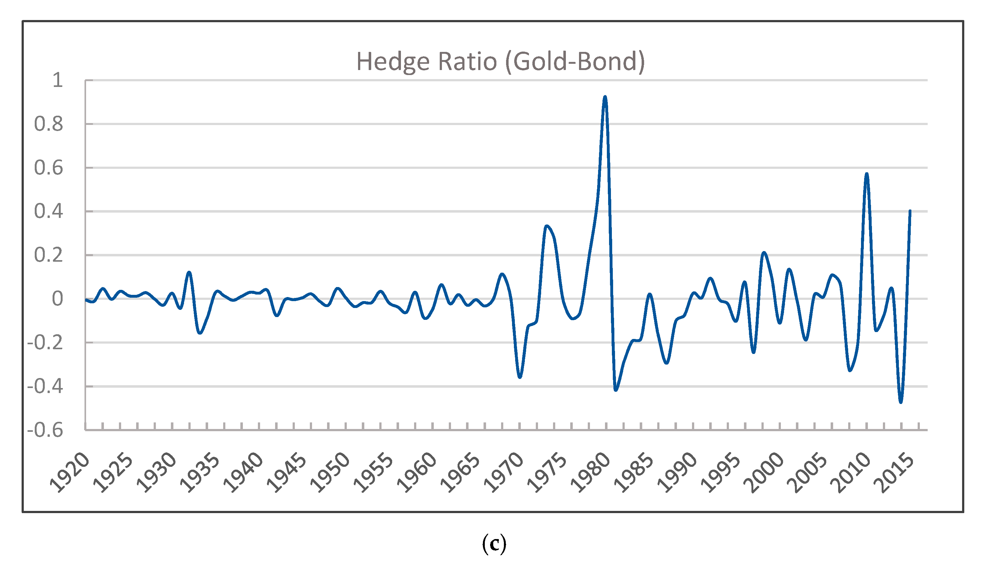
In Table 8, we summarize the average of optimal portfolio weights and hedge ratios over the sample period. The time-varying optimal hedging ratios are presented in Figure 8.
As shown in Table 8, the hedge ratios of portfolios are very close to zero, indicating the hedging effectiveness of gold as a hedge asset in the portfolio. Thus, the inclusion of gold in a diversified portfolio of the other three assets increases the risk-adjusted performance of the resulting portfolio. The negative hedging ratio reflects the fact that asset prices move in opposite directions in the short term. The weight of the gold–stock portfolio means that in a 1-unit portfolio of gold and stock, 58.8% should be invested in gold, with the remaining 41.2% should be invested in stocks. Similarly, for a 1-unit portfolio of gold and oil, 65.2% is invested in gold, and 34.8% in oil. However, in a 1-unit portfolio of gold and bond, 72.7% should be invested in gold and 27.3% in bonds, suggesting that investors prefer gold rather than bonds during periods of financial turmoil. It is worth noting that during the periods of rare disaster risks, investors are likely to invest more in gold than in the other three assets in their portfolio.
As shown in Figure 8, the hedging ratios are relatively stable in most periods and fluctuate around a value of zero, indicating that the constructed portfolio has good hedging effectiveness. However, there are some large fluctuations in hedging ratios from 1970–1980, suggesting that the role of gold in diversified portfolios is likely to change in the presence of the large fluctuations in gold prices, which may be due to the collapse of the Bretton Woods System and the cancellation of the dollar’s convertibility into gold during the 1970s. In periods of high hedging ratio, the hedgers are required to adjust their future positions frequently.
Moreover, we use the method proposed by Ku et al. [58] to check the effectiveness of portfolio diversification. The hedging errors (HE) are defined as: , where represents the variance of the returns on the gold–stock/bond/oil portfolio; is the variance of the returns on the gold. A higher HE ratio indicates that hedging is more effective in reducing the variance of the portfolio; namely, the portfolio can be regarded as an effective hedging strategy.
Table 9 summarizes the results of hedging effectiveness. As shown in Table 9, the portfolio consisting of gold and stock has the largest HE ratio of 44.3%. Therefore, the risk of hedging gold is more effective on stock returns than on bond or oil returns, indicating that the introduction of gold into the stock portfolio can significantly improve its risk–return performance. As for oil, the HE of the portfolio is negative, which may be due to the higher variance of its portfolio returns.
6. Conclusions
In this paper, we aim to provide a flexible framework for the estimation of the time variation in rare disaster risk, and thus to further investigate the role of rare disaster risk in the price dynamics of major commodity and financial assets. First, we apply the approach proposed by Berkman et al. [6] to construct the crisis severity index by aggregating the values of six crisis indicators. Next, we use VAR approaches to investigate the responses of asset markets to the shock of rare disasters, as well as to quantify the fraction of asset volatility attributed to rare disaster risk. Moreover, the possibly nonlinear causal effects of rare disaster risk on asset returns and volatility are examined based on a nonparametric causality-in-quantiles method. We further compare the differences in the effects of rare disaster risks between commodity and financial assets. In addition, the diversified portfolios and the time-varying hedging ratios are constructed to provide the optimal risk hedging strategy for investors. All the findings provide insights into uncovering the role of rare disaster risk in determining the dynamic nature of asset prices.
Our main empirical results are as follows: First, there exists a drastic time variation in the movements of international political crises over the sample period of 1918–2015. We also find substantial differences in the fluctuations of the asset returns, as well as the volatility across major assets in the nearly century-long history. Second, we find a different pattern of the time-varying effects of rare disaster risk on asset markets. The evolution of the impulse responses to rare disaster risk differs greatly between commodity and financial assets over the sample period: the responses are generally positive for commodity except in the recent two decades, whereas they are negative for financial assets. In addition, disaster risk exerts a more intense and persistent influence on oil and stock markets, when compared to gold and bond markets. Third, rare disaster risk is more likely to affect asset market volatility rather than returns. There is no significant evidence of nonlinear causality between rare disaster risk and asset returns at different quantiles, except for crude oil. In contrast, rare disaster risk has a significant nonlinear causal impact on the volatility of asset returns, with some exceptions for the extreme low or high quantiles. In general, we demonstrate a large difference in the role of rare disaster risk between commodity and financial assets.
Our findings have important policy implications. First, understanding the difference of the reactions to rare disaster risk between financial and commodity assets may be of particular interest to financial investors in terms of asset allocation and risk management decisions. The empirical evidence sheds light on the fact that gold can be used as a hedge against other assets during periods of economic turmoil or political crises. In particular, for investment portfolios, the risk hedging of gold is more effective on stock returns than on bonds and oil. Second, the empirical results indicate that close attention to the impact of rare disaster risks should be paid by financial investors as well as policymakers. As rare disaster risk has a strong impact on the fluctuations of commodity and financial markets, it implies that it is necessary to take measures and stage interventions for policymakers to stabilize asset markets, and thus the financial system. This might lead to raising good public expectations and restoring market confidence, thereby reducing the impact of rare disaster risk shocks. For financial investors, it is also crucial to give importance to assessing the impact of disaster events on asset prices when aiming to minimize their investment risk. Financial investors should be aware that rare disaster risks might lead to disruptive fluctuations of asset markets, and furthermore, have a severe impact on their investments.
This study has several limitations and thus also offers some avenues for future research. First, our paper uses low-frequency (i.e., annual) data to investigate the relationship between rare disaster risk and asset prices from a long-term perspective. This is limited to capturing the characteristics of the dynamic relationship; in particular, the short-term responses of high-frequency asset prices to rare disaster shocks. One interesting direction for future research is to explore the role of rare disaster risk in asset markets in both short- and long-term perspectives simultaneously when using the mixed-frequency data model, which allows one to incorporate higher frequency asset prices (such as daily data) with low-frequency rare disaster risk (such as monthly, quarterly, or annual data). Second, the outbreak of the current COVID-19 pandemic (as a special type of rare disaster risk) has a substantial impact on the fluctuations as well as the connectedness among globally traded commodity and financial markets. A natural extension of the research is to explore the role of the COVID-19 pandemic in the fluctuations, as well as risk transmission across commodities and financial assets markets. Third, due to the lack of long-term crisis data for certain categories of crises, the constructed measure of crisis severity index is based on the major representative crisis dimensions, rather than all crisis dimensions in the ICB’s crisis database. One interesting direction is to further understand the role of disaster risk via using all crisis dimensions of the ICB database to construct a more comprehensive proxy of disaster risk in recent decades.
Author Contributions
Conceptualization, methodology, writing, writing—review and editing, supervision, P.C.; methodology, software, formal analysis, investigation, writing, writing—review and editing, T.H. All authors have read and agreed to the published version of the manuscript.
Funding
Peng Chen is grateful for the grant from the Humanities and Social Science Foundation of the Ministry of Education of China (No. 20YJC790012) and the National Natural Science Foundation of China (No. 72071095).
Institutional Review Board Statement
Not applicable.
Informed Consent Statement
Not applicable.
Data Availability Statement
The crises data were obtained from the International Crisis Behavior (ICB) database (https://sites.duke.edu/icbdata/ (accessed on 16 October 2018).); data on stock price indices and bond indices were taken from Robert Shiller’s publication Irrational Exuberance; data of oil prices in dollars are from British Petroleum and data of gold prices in dollars are from the National Mining Association. All the data are also available from the authors on request.
Conflicts of Interest
The authors declare no conflict of interest.
References
- Rietz, T.A. The equity risk premium a solution. J. Monet. Econ. 1988, 22, 117–131. [Google Scholar] [CrossRef]
- Gabaix, X. Variable Rare Disasters: A Tractable Theory of Ten Puzzles in Macro-Finance. Am. Econ. Rev. 2008, 98, 64–67. [Google Scholar] [CrossRef] [Green Version]
- Barro, R.J. Rare disasters and asset markets in the twentieth century. Q. J. Econ. 2006, 121, 823–866. [Google Scholar] [CrossRef]
- Gabaix, X. Variable Rare Disasters: An Exactly Solved Framework for Ten Puzzles in Macro-Finance. Q. J. Econ. 2012, 127, 645–700. [Google Scholar] [CrossRef] [Green Version]
- Veronesi, P. The Peso problem hypothesis and stock market returns. J. Econ. Dyn. Control 2004, 28, 707–725. [Google Scholar] [CrossRef]
- Berkman, H.; Jacobsen, B.; Lee, J.B. Time-varying rare disaster risk and stock returns. J. Financ. Econ. 2011, 101, 313–332. [Google Scholar] [CrossRef]
- Wachter, J.A. Can time-varying risk of rare disasters explain aggregate stock market volatility? J. Financ. 2013, 68, 987–1035. [Google Scholar] [CrossRef] [Green Version]
- Seo, S.B.; Wachter, J.A. Option prices in a model with stochastic disaster risk. Manag. Sci. 2019, 65, 3449–3469. [Google Scholar] [CrossRef] [Green Version]
- Zhang, Q. One hundred years of rare disaster concerns and commodity prices. J. Futures Mark. 2021, 41, 1891–1915. [Google Scholar] [CrossRef]
- Farhi, E.; Gabaix, X. Rare Disasters and Exchange Rates. Q. J. Econ. 2016, 131, 1–52. [Google Scholar] [CrossRef] [Green Version]
- Berkman, H.; Jacobsen, B.; Lee, J.B. Rare disaster risk and the expected equity risk premium. Account. Financ. 2015, 57, 351–372. [Google Scholar] [CrossRef]
- Lee, C.C.; Lee, C.C.; Li, Y.Y. Oil price shocks, geopolitical risks, and green bond market dynamics. N. Am. J. Econ. Financ. 2021, 55, 101309. [Google Scholar] [CrossRef]
- Demirer, R.; Gupta, R.; Suleman, T.; Wohar, M.E. Time-varying rare disaster risks, oil returns and volatility. Energy Econ. 2018, 75, 239–248. [Google Scholar] [CrossRef] [Green Version]
- Cunado, J.; Gupta, R.; Lau, C.K.M.; Sheng, X. Time-Varying Impact of Geopolitical Risks on Oil Prices. Def. Peace Econ. 2020, 31, 692–706. [Google Scholar] [CrossRef]
- Gkillas, K.; Gupta, R.; Pierdzioch, C. Forecasting (downside and upside) realized exchange-rate volatility: Is there a role for realized skewness and kurtosis? Phys. A Stat. Mech. Appl. 2019, 532, 121867. [Google Scholar] [CrossRef]
- Salisu, A.A.; Cunado, J.; Gupta, R. Geopolitical risks and historical exchange rate volatility of the BRICS. Int. Rev. Econ. Financ. 2022, 77, 179–190. [Google Scholar] [CrossRef]
- Sharif, A.; Aloui, C.; Yarovaya, L. COVID-19 pandemic, oil prices, stock market, geopolitical risk and policy uncertainty nexus in the US economy: Fresh evidence from the wavelet-based approach. Int. Rev. Financ. Anal. 2020, 70, 101496. [Google Scholar] [CrossRef]
- Liu, L.; Wang, E.Z.; Lee, C.C. Impact of the COVID-19 pandemic on the crude oil and stock markets in the US: A time-varying analysis. Energy Res. Lett. 2020, 1, 13154. [Google Scholar] [CrossRef]
- Umar, Z.; Jareño, F.; Escribano, A. Dynamic return and volatility connectedness for dominant agricultural commodity markets during the COVID-19 pandemic era. Appl. Econ. 2021, 1–25. [Google Scholar] [CrossRef]
- Barro, R.J.; Jin, T. On the Size Distribution of Macroeconomic Disasters. Econometrica 2011, 79, 1567–1589. [Google Scholar] [CrossRef] [Green Version]
- Balcilar, M.; Bekiros, S.; Gupta, R. The role of news-based uncertainty indices in predicting oil markets: A hybrid nonparametric quantile causality method. Empir. Econ. 2017, 53, 879–889. [Google Scholar] [CrossRef] [Green Version]
- Gourio, F. Time-Varying Risk of Disaster, Time-Varying Risk Premia, and Macroeconomic Dynamics. In Time-Varying Risk Premia, and Macroeconomic Dynamics (18 March 2009); SSRN: New York, NY, USA, 2009. [Google Scholar]
- Gourio, F.; Siemer, M.; Verdelhan, A. International risk cycles. J. Int. Econ. 2013, 89, 471–484. [Google Scholar] [CrossRef] [Green Version]
- Tsai, J.; Wachter, J.A. Rare booms and disasters in a multisector endowment economy. Rev. Financ. Stud. 2016, 29, 1113–1169. [Google Scholar] [CrossRef] [Green Version]
- Barro, R.J.; Misra, S. Gold Returns. Econ. J. 2016, 126, 1293–1317. [Google Scholar] [CrossRef]
- Barro, R.J.; Liao, G.Y. Rare disaster probability and options pricing. J. Financ. Econ. 2021, 139, 750–769. [Google Scholar] [CrossRef]
- Skoufias, E. Economic Crises and Natural Disasters: Coping Strategies and Policy Implications. World Dev. 2003, 31, 1087–1102. [Google Scholar] [CrossRef]
- Huang, T.; Wu, F.; Yu, J.; Zhang, B. Political risk and dividend policy: Evidence from international political crises. J. Int. Bus. Stud. 2015, 46, 574–595. [Google Scholar] [CrossRef]
- Meng, Y.W.; Imran, M.; Zakaria, M.; Linrong, Z.; Farooq, M.U.; Muhammad, S.K. Impact of terrorism and political instability on equity premium: Evidence from Pakistan. Phys. A Stat. Mech. Appl. 2018, 492, 1753–1762. [Google Scholar] [CrossRef]
- Gkillas, K.; Floros, C.; Suleman, M.T. Quantile dependencies between discontinuities and time-varying rare disaster risks. Eur. J. Financ. 2021, 27, 932–962. [Google Scholar] [CrossRef]
- Gupta, R.; Suleman, T.; Wohar, M.E. The role of time-varying rare disaster risks in predicting bond returns and volatility. Rev. Financ. Econ. 2019, 37, 327–340. [Google Scholar] [CrossRef]
- van Eyden, R.; Gupta, R.; Nel, J.; Bouri, E. Rare Disaster Risks and Volatility of the Term-Structure of US Treasury Securities: The Role of El Nino and La Nina Events (No. 202155); Dept. of Economics Working Paper Series; University of Pretoria: Pretoria, South Africa, 2021. [Google Scholar]
- Demirer, R.; Gupta, R.; Nel, J.; Pierdzioch, C. Effect of rare disaster risks on crude oil: Evidence from El Niño from over 145 years of data. Theor. Appl. Climatol. 2021, 147, 691–699. [Google Scholar] [CrossRef]
- Adekoya, O.B.; Oliyide, J.A. How COVID-19 drives connectedness among commodity and financial markets: Evidence from TVP-VAR and causality-in-quantiles techniques. Resour. Policy 2020, 70, 101898. [Google Scholar] [CrossRef] [PubMed]
- Bissoondoyal-Bheenick, E.; Do, H.; Hu, X.; Zhong, A. Learning from SARS: Return and volatility connectedness in COVID-19. Financ. Res. Lett. 2021, 41, 101796. [Google Scholar] [CrossRef] [PubMed]
- Mensi, W.; Sensoy, A.; Vo, X.V.; Kang, S.H. Impact of COVID-19 outbreak on asymmetric multifractality of gold and oil prices. Resour. Policy 2020, 69, 101829. [Google Scholar] [CrossRef] [PubMed]
- Harjoto, M.A.; Rossi, F.; Lee, R.; Sergi, B.S. How do equity markets react to COVID-19? Evidence from emerging and developed countries. J. Econ. Bus. 2021, 115, 105966. [Google Scholar] [CrossRef] [PubMed]
- Primiceri, G.E. Time varying structural vector autoregressions and monetary policy. Rev. Econ. Stud. 2005, 72, 821–852. [Google Scholar] [CrossRef]
- Nakajima, J. Time-Varying Parameter VAR Model with Stochastic Volatility: An Overview of Methodology and Empirical Applications. Monet. Econ. Stud. 2011, 29, 107–142. [Google Scholar]
- Degiannakis, S.; Filis, G.; Panagiotakopoulou, S. Oil price shocks and uncertainty: How stable is their relationship over time? Econ. Model. 2018, 72, 42–53. [Google Scholar] [CrossRef] [Green Version]
- Paul, P. The time-varying effect of monetary policy on asset prices. Rev. Econ. Stat. 2020, 102, 690–704. [Google Scholar] [CrossRef] [Green Version]
- Nishiyama, Y.; Hitomi, K.; Kawasaki, Y.; Jeong, K. A consistent nonparametric test for nonlinear causality—Specification in time series regression. J. Econ. 2011, 165, 112–127. [Google Scholar] [CrossRef] [Green Version]
- Jebabli, I.; Arouri, M.; Teulon, F. On the effects of world stock market and oil price shocks on food prices: An empirical investigation based on TVP-VAR models with stochastic volatility. Energy Econ. 2014, 45, 66–98. [Google Scholar] [CrossRef]
- Chib, S.; Greenberg, E. Hierarchical analysis of SUR models with extensions to correlated serial errors and time-varying parameter models. J. Econ. 1995, 68, 339–360. [Google Scholar] [CrossRef]
- Chib, S. Markov Chain Monte Carlo Methods: Computation and Inference. Handb. Econom. 2001, 5, 3569–3649. [Google Scholar] [CrossRef]
- Kim, S.; Shepherd, N.; Chib, S. Stochastic Volatility: Likelihood Inference and Comparison with ARCH Models. Rev. Econ. Stud. 1998, 65, 361–393. [Google Scholar] [CrossRef]
- Omori, Y.; Chib, S.; Shephard, N.; Nakajima, J. Stochastic volatility with leverage: Fast and efficient likelihood inference. J. Econ. 2007, 140, 425–449. [Google Scholar] [CrossRef] [Green Version]
- Jeong, K.; Härdle, W.K.; Song, S. A consistent nonparametric test for causality in quantile. Econ. Theory 2012, 28, 861–887. [Google Scholar] [CrossRef] [Green Version]
- Sim, N.; Zhou, H. Oil prices, US stock return, and the dependence between their quantiles. J. Bank. Financ. 2015, 55, 1–8. [Google Scholar] [CrossRef]
- Baur, D.G.; Lucey, B.M. Is gold a hedge or a safe haven? An analysis of stocks, bonds and gold. Financ. Rev. 2010, 45, 217–229. [Google Scholar] [CrossRef]
- Goyenko, R.Y.; Ukhov, A.D. Stock and bond market liquidity: A long-run empirical analysis. J. Financ. Quant. Anal. 2009, 44, 189–212. [Google Scholar] [CrossRef] [Green Version]
- Lieber, R.J. Oil and power after the Gulf War. Int. Secur. 1992, 17, 155–176. [Google Scholar] [CrossRef]
- Rigobon, R.; Sack, B. The effects of war risk on US financial markets. J. Bank. Financ. 2005, 29, 1769–1789. [Google Scholar] [CrossRef] [Green Version]
- Leigh, A.; Wolfers, J.; Zitzewitz, E. What Do Financial Markets Think of War in Iraq? Working Paper No. 9587; National Bureau of Economic Research: Cambridge, MA, USA, 2003. [Google Scholar] [CrossRef]
- Urquhart, A. An Empirical Analysis of the Adaptive Market Hypothesis and Investor Sentiment in Extreme Circumstances. Doctoral Dissertation, Newcastle University, Newcastle, UK, 2013. [Google Scholar]
- Kroner, K.F.; Ng, V.K. Modeling asymmetric movement of asset prices. Rev. Financ. Stud. 1998, 11, 844–871. [Google Scholar] [CrossRef]
- Kroner, K.F.; Sultan, J. Time-Varying Distributions and Dynamic Hedging with Foreign Currency Futures. J. Financ. Quant. Anal. 1993, 28, 535. [Google Scholar] [CrossRef]
- Ku, Y.H.H.; Chen, H.C.; Chen, K. On the application of the dynamic conditional correlation model in estimating optimal time-varying hedge ratios. Appl. Econ. Lett. 2007, 14, 503–509. [Google Scholar] [CrossRef]
Figure 1.
Annual number of international crises and crisis severity index.

Figure 2.
Estimation results for selected parameters in the TVP–VAR model.

Figure 3.
Simultaneous impulse response of asset returns to CSI shocks. Notes: Figure 3 presents the results of simultaneous impulse response of asset returns to CSI shocks for (a) stock, (b) bond, (c) oil, and (d) gold, respectively.
Figure 3.
Simultaneous impulse response of asset returns to CSI shocks. Notes: Figure 3 presents the results of simultaneous impulse response of asset returns to CSI shocks for (a) stock, (b) bond, (c) oil, and (d) gold, respectively.

Figure 4.
Impulse response of asset returns to CSI shock after 3 years.

Figure 5.
Impulse response of asset returns to CSI shock after 5 years.

Figure 6.
Impulse responses of assets return to disaster risk shocks in particular periods. Notes: The figure presents the impulse responses of asset return to disaster risk shocks in (a) 1950, (b) 1981, (c) 1992, and (d) 2007, respectively. The responses of asset return tend to be nearly zero after the sixth period for the case of 1950, whereas they are nearly zero after the fourth period for the cases of 1981 and 1992, and nearly zero after the third period for the case of 2007.


Figure 7.
Causality-in-quantiles of asset prices to rare disaster risk. Notes: Figure 7 presents the results of causality-in-quantiles of asset prices to rare disaster risk for (a) stock, (b) bond, (c) oil, and (d) gold, respectively. Horizontal axis refers to the quantiles; vertical axis refers to the test statistics corresponding to the null hypothesis that rare disaster risk does not cause Granger asset prices. The dark solid line represents the standardized test statistics of the results based on the causality-in-quantiles tests for asset returns or volatility, respectively. The grey horizontal line is the 5% critical value, around 1.96 (if the dark solid line is above the grey horizontal line (denoting critical value), indicating a significant causality effect of disaster risk on asset prices; otherwise, indicating there is no significant causality effect).

Figure 8.
Dynamic hedging ratio . Notes: Figure 8 shows the results of dynamic hedge ratios between (a) gold and stock, (b) gold and oil, and (c) gold and bond, respectively.
Figure 8.
Dynamic hedging ratio . Notes: Figure 8 shows the results of dynamic hedge ratios between (a) gold and stock, (b) gold and oil, and (c) gold and bond, respectively.


Table 1.
The definition of six dummy variables.
| Variables | Description | Value |
|---|---|---|
| BREAK ) | Crisis that began with a violent act | value 9: Violent act |
| VIOL ) | Violence used during the crisis or full-scale wars | value 3: Serious clashes; value 4: Full-scale wars. |
| WAR ) | Full-scale wars | value 4: Full-scale wars. |
| GRAVCR ) | Subset of “Gravity of value threat”—grave threat | value 3: Territorial threat; value 5: Threat of grave damage; value 6: Threat to existence. |
| PROTRAC ) | - | value 3: Long power protracted conflict. |
| GPINV ) | Great power or Superpower is involved on both sides of conflict | value 3: One or more powers high involvement; value 4: One or two powers as crisis actors, the others low or no involvement; value 5: One or two powers as crisis actor, the others high, low or no involvement; value 6: More than two powers as crisis actors, the other low or no involvement; value 7: More than two powers as crisis actors, the other high, low or no involvement |
Table 2.
Summary statistics of CSI subsets across categories.
| Variables | BREAK | VIOL | WAR | GRAVCR | MAJPOW | PROTRAC |
|---|---|---|---|---|---|---|
| Total | 194 | 211 | 83 | 258 | 159 | 66 |
Note: Here Total refers to the total number of crisis events (i.e., crisis categories) over the sample periods.
Table 3.
Summary statistics.
| Mean | Median | Max | Min | Std. Dev. | Skewness | Kurtosis | |
|---|---|---|---|---|---|---|---|
| CSI | 62.316 | 54.500 | 279.000 | 0.000 | 43.737 | 1.797 | 9.126 |
| Returns | |||||||
| Stock | 5.466 | 8.970 | 39.649 | −65.508 | 18.775 | −0.978 | 4.507 |
| Bond | −0.827 | 0.405 | 40.372 | −54.280 | 16.400 | −0.297 | 4.005 |
| Oil | 3.586 | 0.000 | 125.839 | −64.706 | 26.118 | 0.774 | 8.191 |
| Gold | 4.197 | 0.048 | 69.804 | −29.040 | 15.400 | 1.421 | 6.658 |
Notes: Crisis Severity Index (CSI) is constructed of six crisis dimensions, which are introduced above. The annual returns on assets are defined as logarithmic a difference of asset prices (measured in percent), i.e., ∗100%.
Table 4.
Variance decomposition of asset returns due to rare disaster risk.
| Period | Stock | Bond | Oil | Gold |
|---|---|---|---|---|
| 1 | 0.39 | 0.00 | 3.23 | 0.36 |
| 2 | 0.40 | 2.19 | 3.14 | 1.49 |
| 3 | 8.08 | 2.01 | 2.74 | 2.57 |
| 4 | 10.09 | 2.58 | 2.69 | 4.15 |
| 5 | 10.02 | 2.46 | 7.34 | 3.93 |
| 10 | 13.17 | 2.79 | 9.70 | 4.55 |
| 15 | 13.04 | 2.93 | 9.83 | 4.85 |
| 20 | 13.07 | 2.97 | 9.85 | 4.85 |
| 25 | 13.07 | 2.97 | 9.85 | 4.85 |
| 30 | 13.07 | 2.97 | 9.85 | 4.85 |
Notes: The VAR system consists of rare disaster risk, stock, bond, oil, and gold. The table reports the estimation results which are based on the Cholesky variance decompositions for different asset returns. The shares attributable to rare disaster risk for different assets at different time durations are reported in the table, respectively.
Table 5.
Estimates of TVP-VAR model.
| Parameter | Mean | Std Dev. | 95% U | 95% L | Geweke CD | Inefficiency |
|---|---|---|---|---|---|---|
| 0.2305 | 0.0414 | 0.1575 | 0.32 | 0.734 | 14.13 | |
| 0.0023 | 0.0003 | 0.0018 | 0.0029 | 0.078 | 5.35 | |
| 0.0059 | 0.0017 | 0.0035 | 0.0102 | 0.243 | 40.69 | |
| 0.0087 | 0.0032 | 0.0043 | 0.0166 | 0.000 | 87.62 | |
| 0.0055 | 0.0015 | 0.0034 | 0.0094 | 0.812 | 27.09 | |
| 0.0056 | 0.0017 | 0.0034 | 0.0101 | 0.971 | 39.11 |
Notes: Here, 95% U and 95% L refer to the lower and upper bounds of 95% confidence intervals of the estimates of the posterior distributions. Geweke CD is the convergence diagnostic (CD) statistics suggested by Geweke, which can be used to examine the convergence in the Markov chain. Inefficiency represents the inefficiency factor of the MCMC algorithm in replicating the posterior draws.
Table 6.
Causality-in-quantiles result.
| Quantiles | Stock–Mean | Stock–Variance | Bond–Mean | Bond–Variance | Oil–Mean | Oil–Variance | Gold–Mean | Gold–Variance |
|---|---|---|---|---|---|---|---|---|
| 0.05 | 0.04 | 1.64 | 0.00 | 1.38 | 0.79 | 5.74 | 0.15 | 3.93 |
| 0.1 | 0.00 | 2.36 | 0.04 | 1.65 | 1.44 | 3.89 | 0.19 | 2.95 |
| 0.15 | 0.01 | 2.50 | 0.00 | 1.73 | 1.12 | 3.19 | 0.13 | 3.00 |
| 0.2 | 0.01 | 2.84 | 0.01 | 2.06 | 1.13 | 3.16 | 0.18 | 3.14 |
| 0.25 | 0.01 | 3.44 | 0.01 | 2.01 | 1.06 | 3.18 | 0.20 | 3.05 |
| 0.3 | 0.01 | 3.40 | 0.01 | 2.26 | 1.00 | 3.19 | 0.28 | 3.13 |
| 0.35 | 0.02 | 3.30 | 0.02 | 2.71 | 0.99 | 3.39 | 0.20 | 3.63 |
| 0.4 | 0.00 | 3.39 | 0.02 | 2.44 | 2.96 | 3.35 | 0.10 | 3.75 |
| 0.45 | 0.03 | 3.30 | 0.03 | 2.49 | 1.94 | 3.29 | 0.71 | 3.60 |
| 0.5 | 0.00 | 3.16 | 0.00 | 2.42 | 1.25 | 3.23 | 0.23 | 3.17 |
| 0.55 | 0.01 | 3.03 | 0.01 | 3.05 | 0.77 | 3.18 | 0.19 | 2.89 |
| 0.6 | 0.01 | 3.03 | 0.01 | 2.67 | 0.82 | 3.33 | 0.40 | 2.74 |
| 0.65 | 0.01 | 2.99 | 0.00 | 2.57 | 0.73 | 3.11 | 0.24 | 2.50 |
| 0.7 | 0.02 | 2.64 | 0.00 | 2.56 | 0.45 | 2.97 | 0.66 | 2.11 |
| 0.75 | 0.03 | 2.38 | 0.03 | 2.42 | 0.80 | 2.51 | 1.24 | 2.00 |
| 0.8 | 0.04 | 2.34 | 0.00 | 1.95 | 0.89 | 2.35 | 0.66 | 1.58 |
| 0.85 | 0.00 | 1.76 | 0.01 | 1.66 | 0.72 | 2.32 | 0.54 | 1.25 |
| 0.9 | 0.01 | 1.46 | 0.00 | 1.19 | 0.38 | 1.91 | 0.61 | 0.99 |
| 0.95 | 0.00 | 1.42 | 0.02 | 0.66 | 0.26 | 1.71 | 0.19 | 0.33 |
Table 7.
Significant quantiles of asset returns in mean and variance.
| Stock | Bond | Oil | Gold | |
|---|---|---|---|---|
| Mean | - | - | 0.35–0.45 | - |
| Variance | 0.10–0.85 | 0.20–0.80 | 0–0.85 | 0–0.75 |
Table 8.
Estimates of the weight of portfolios.
| Portfolios | |||
|---|---|---|---|
| Gold–Stock | 0.588 | 0.412 | −0.009 |
| Gold–Oil | 0.652 | 0.348 | 0.099 |
| Gold–Bond | 0.727 | 0.273 | −0.004 |
Table 9.
Hedging errors.
| Portfolios | Gold–Stock | Gold–Oil | Gold–Bond |
|---|---|---|---|
| Variance | 0.013 | 0.026 | 0.014 |
| HE | 0.443 | −0.113 | 0.397 |
Publisher’s Note: MDPI stays neutral with regard to jurisdictional claims in published maps and institutional affiliations. |
© 2022 by the authors. Licensee MDPI, Basel, Switzerland. This article is an open access article distributed under the terms and conditions of the Creative Commons Attribution (CC BY) license (https://creativecommons.org/licenses/by/4.0/).
Share and Cite
MDPI and ACS Style
Chen, P.; Huang, T. Do Commodities React More to Time-Varying Rare Disaster Risk? A Comparison of Commodity and Financial Assets. Mathematics 2022, 10, 445. https://0-doi-org.brum.beds.ac.uk/10.3390/math10030445
AMA Style
Chen P, Huang T. Do Commodities React More to Time-Varying Rare Disaster Risk? A Comparison of Commodity and Financial Assets. Mathematics. 2022; 10(3):445. https://0-doi-org.brum.beds.ac.uk/10.3390/math10030445
Chicago/Turabian StyleChen, Peng, and Ting Huang. 2022. "Do Commodities React More to Time-Varying Rare Disaster Risk? A Comparison of Commodity and Financial Assets" Mathematics 10, no. 3: 445. https://0-doi-org.brum.beds.ac.uk/10.3390/math10030445
Note that from the first issue of 2016, this journal uses article numbers instead of page numbers. See further details here.