Dynamical Analysis of a Delayed Diffusive Predator–Prey Model with Additional Food Provided and Anti-Predator Behavior

Abstract

We studied a delayed predator–prey model with diffusion and anti-predator behavior. Assume that additional food is provided for predator population. Then the stability of the positive equilibrium is considered. The existence of Hopf bifurcation is also discussed based on the Hopf bifurcation theory. The property of Hopf bifurcation is derived through the theory of center manifold and normal form method. Finally, we analyze the effect of time delay on the model through numerical simulations.

1. Introduction

The interaction between predator and prey is ordinary and widespread in nature, it could affect the ecological balance. There exists an interesting phenomena in prey called anti-predator behavior, that is, adult prey kills young predators in order to overcome the predation pressure and improve their population density in the future [1,2,3,4,5]. Sometimes, this behavior may lead to species outbreak and do harm to the stability of the ecosystem. Hence, providing additional food for predator is a manner to avoid it [6]. Complex dynamics would be shown if anti-predator behavior happens.

The following predator–prey model (1) was proposed in [7]. In the absence of predators, the growth of the prey population follows the logistic equation. Assume Holling IV functional response exists in this system.

$$\begin{array}{c}\hfill \left\{\begin{array}{c}\frac{\mathrm{d}N}{\mathrm{d}T}=rN(1-\frac{N}{K})-\frac{cNP}{(q{N}^2+1)(a+\alpha {\eta }_{1}A)}\hfill \\ \frac{\mathrm{d}P}{\mathrm{d}T}=\frac{b\left(N+(q{N}^2+1){\eta }_{1}A\right)P}{(q{N}^2+1)(a+\alpha {\eta }_{1}A)}-mP-\overline{\eta }NP\hfill \end{array}\right.\end{array}$$

(1)

All parameters are positive and their biological description could be found from [7] as

Table 1. Biological description of parameters in model (1).

Parameter	Definition	Parameter	Definition
T	Time	r	Prey intrinsic growth rate
N	Prey population	P	Predator population
K	Carrying capacity of prey	c	Maximum rate of predation
b	Maximum growth rate of predator	m	Predator mortality rate
q	Group defense in prey	$\overline{\eta }$	Rate of anti-predator behavior
$\overline{{\eta }_1}$	Effectual ability of the predators to detect additional food relative to the prey	A	Quantity of additional food provided to the predators
a	Normalization coefficient relating the densities of prey and predator to the environment in which they interact	$\alpha$	Ratio between the handling times towards the additional food and the prey

. In addition to the main food prey u, the predator has additional food sources A in the model (1). An the term $\overline{\eta }NP$ represents the anti-predator behavior in prey. K. D. Prasad et al. [7] investigated various bifurcations of the system (1), including Bogd- anov–Takens bifurcation, Saddle-node bifurcation, and Hopf bifurcation. They also considered the global dynamics of this system.

The predator–prey model has important research value in biomathematics; therefore, many experts have investigated it and obtained plenty of valuable results [8,9,10,11,12]. For example, time delay is an element that cannot be ignored in population dynamics. In nature, the development of population is not only related to the current state, but also related to the past time state, which is often called time delay. Generally, time delay often causes instability and periodic oscillation. In this paper, we are going to study the effect of time delay on the model (1), and intend to observe whether some new dynamic phenomenon happens.

Further, the distribution of prey and predator are usually nonhomogeneous and different concentration levels of them would cause different population movements [13]; then, the diffusion phenomenon occurs. Some scholars provide different approaches of mathematical modeling of some ecological interaction in the presence of spatial diffusion [14,15,16,17]. In [15], the authors considered a predator–prey model with herd behavior and the cross-diffusion and fear effect, they mainly studied the Turing patterns and Turing–Hopf bifurcation induced by cross-diffusion. In [17], S. Djilali and S. Bentout studied a diffusive predator–prey model in the presence of predator rivalry and prey social behavior. They mainly studied the stability and Hopf bifurcation, and they show the nonhomogeneous periodic solution induced by diffusion. These works show that the diffusion term often causes the Turing pattern, spatial non-uniform periodic oscillation and so on.

Inspired by the above works, we incorporate the diffusion term and time delay to the model (1) and investigate the following model (2). We mainly study the Hopf bifurcation by the theory of center manifold and normal form method by using time delay as the bifurcation parameter.

$$\begin{array}{c}\hfill \left\{\begin{array}{c}\frac{\partial N(x,t)}{\partial t}=D_1\Delta N+rN(1-\frac{N(T-T_1)}{K})-\frac{cNP}{(q{N}^2+1)(a+\alpha {\eta }_{1}A)}\hfill \\ \frac{\partial P(x,t)}{\partial t}=D_2\Delta P+\frac{b\left(N+(q{N}^2+1){\eta }_{1}A\right)P}{(q{N}^2+1)(a+\alpha {\eta }_{1}A)}-mP-\overline{\eta }NP\hfill \end{array}\right.\end{array}$$

(2)

where $D_1$ and $D_2$ represents the diffusion coefficients of prey and predator, respectively. Suppose there exists a time delay $T_1$, which denotes the resource limitation of the prey logistic equation. It is convenient to non-dimensionalize the model with the transformations as $u=\frac{N}{a}$, $v=\frac{CP}{ar}$, and $t=rT$. Then, the following model is obtained.

$$\begin{array}{c}\hfill \left\{\begin{array}{cc}\frac{\partial u(x,t)}{\partial t}=d_1\Delta u+u(1-\frac{u(t-\tau )}{\gamma })-\frac{uv}{(w{u}^2+1)(1+\alpha ϵ)},\hfill & x\in (0,l\pi ),t>0,\hfill \\ \frac{\partial v(x,t)}{\partial t}=d_2\Delta v+\frac{\beta \left(u+(w{u}^2+1)ϵ\right)v}{(w{u}^2+1)(1+\alpha ϵ)}-\delta v-suv,\hfill & x\in (0,l\pi ),t>0,\hfill \\ u_x(0,t)=v_x(0,t)=0,u_x(l\pi ,t)=v_x(l\pi ,t)=0,\hfill & t>0,\hfill \\ u(x,\theta )=u_0(x,\theta )\ge 0,v(x,\theta )=v_0(x,\theta )\ge 0,\hfill & x\in [0,l\pi ],\theta \in [-\tau ,0].\hfill \end{array}\right.\end{array}$$

(3)

where

$$\gamma =\frac{K}{a},w=q{a}^2,ϵ=\frac{{\eta }_{1}A}{a},\beta =\frac{b}{r},\delta =\frac{m}{r},s=\frac{\overline{\eta }a}{r},d_1=\frac{D_1}{r},d_2=\frac{D_2}{r}.$$

All parameters in the model (3) are non-negative. $\frac{\partial u(x,t)}{\partial t}$ and $\frac{\partial v(x,t)}{\partial t}$ denote the gradient of prey and predator densities, respectively. The boundary condition is Neumann boundary condition, based on the hypothesis that the region where prey and predators live is closed and no prey and predator entering or leaving the region.

In this paper, we mainly study the effect of time delay and diffusion term on the model (3), such as delay inducing instability, homogeneous or inhomogeneous bifurcating periodic solutions. The rest of our paper is divided as follows. In Section 2, the local stability of the equilibrium is studied, some conditions under which Hopf bifurcation occurs are also derived. The property of Hopf bifurcation is investigated in Section 3 and numerical simulations are presented in Section 4. At last, we give a short conclusion.

2. Analysis of the Characteristic Equations

The equilibria of system (3) are the roots of the following equations

$$\begin{array}{c}\hfill \left\{\begin{array}{c}u(1-\frac{u}{\gamma })-\frac{uv}{(w{u}^2+1)(1+\alpha ϵ)}=0,\hfill \\ \frac{\beta \left(u+(w{u}^2+1)ϵ\right)v}{(w{u}^2+1)(1+\alpha ϵ)}-\delta v-suv=0.\hfill \end{array}\right.\end{array}$$

(4)

The existence of positive equilibrium is exactly investigated in [7]. The results are as follows.

Lemma 1.

Ref. [7]For the model (3), the following conclusions about the existence of positive equilibrium are true.

1. 

$(0,0)$ and $(\gamma ,0)$ are two boundary equilibria.

2. 

There exists a unique interior equilibrium $E_1(u_1,v_1)$, when $\beta -s(1+\alpha ϵ)>0,\beta ϵ-\delta (1+\alpha ϵ)\le 0$ and $f\left(u_c\right)<0$, $u_1<\gamma <u_2$.

3. 

There exists two interior equilibria $E_1(u_1,v_1)$ and $E_2(u_2,v_2)$, when $\beta -s(1+\alpha ϵ)>0,\beta ϵ-\delta (1+\alpha ϵ)\le 0$ and $f\left(u_c\right)<0$, $u_1<u_2<\gamma$.

4. 

There exists an instantaneous equilibrium $E_c(u_c,v_c)$, when $\beta -s(1+\alpha ϵ)>0,\beta ϵ-\delta (1+\alpha ϵ)\le 0$ and $f\left(u_c\right)=0$, $u_c<\gamma$.

5. 

There exists one equilibrium $E_2(u_2,v_2)$ if $\beta ϵ-\delta (1+\alpha ϵ)>0$ and $u_2<\gamma$.

where

$$\begin{array}{cc}\hfill f\left(u\right)=& sw(1+\alpha ϵ)u^3-[\beta ϵ-\delta (1+\alpha ϵ)]w{u}^2\hfill \\ \hfill & -[\beta -s(1+\alpha ϵ\left)\right]u-[\beta ϵ-\delta (1+\alpha ϵ\left)\right],\hfill \\ \hfill f^{\prime }\left(u\right)=& 3sw(1+\alpha ϵ)u^2-2w[\beta ϵ-\delta (1+\alpha ϵ)]u\hfill \\ \hfill & -[\beta -s(1+\alpha ϵ\left)\right],\hfill \\ \hfill f^{″}\left(u\right)=& 6sw(1+\alpha ϵ)u-2w[\beta ϵ-\delta (1+\alpha ϵ\left)\right].\hfill \end{array}$$

(5)

Proof of Lemma 1.

Case 1. For $u>0$, suppose $\beta ϵ-\delta (1+\alpha ϵ)\le 0$, then $f^{″}\left(u\right)>0$ and $f\left(0\right)\ge 0$. If $\beta -s(1+\alpha ϵ)>0$, $f\left(u\right)=0$ has a local minimum value at $u_c(u_c>0)$. Because by analyzing $f^{\prime }\left(u\right)$, we know $f\left(u\right)$ is decreasing in $(0,u_c)$ and increasing in $(u_c,+\infty )$. When $f\left(u_c\right)<0$, $f\left(u\right)$ has two positive equilibrium written as $E_1(u_1,v_1)$ and $E_2(u_2,v_2)$ with $0<u_1<u_2$; when $f\left(u_c\right)=0$, $f\left(u\right)$ has only one positive root $E_c(u_c,v_c)$. If $\beta -s(1+\alpha ϵ)\le 0$, then $f^{\prime }\left(u\right)\ge 0$ for all u. Thus, $f\left(u\right)$ has no positive root in $(0,+\infty )$.

Case 2. Suppose $\beta ϵ-\delta (1+\alpha ϵ)>0$, then $f\left(0\right)<0$ and $f^{″}\left(u\right)=0$ admits a positive real root $u_{cc}$. We know $f^{\prime }\left(u\right)$ is decreasing in $(0,u_{cc})$ and increasing in $(u_{cc},+\infty )$. If $\beta -s(1+\alpha ϵ)>0$, easily know $f^{\prime }\left(0\right)<0$. The equation $f\left(u\right)=0$ has one positive real root $u_2$ because its discriminant is either positive or negative. If $\beta -s(1+\alpha ϵ)\le 0$, then $f^{\prime }\left(0\right)>0$. The equation $f\left(u\right)=0$ has one positive real root $u_2$ and a pair of complex conjugate roots because its discriminant is always negative. To know the detailed discussion, one can refer to the literature [7]. □

Next, suppose the model (3) has a positive equilibrium $P=(u_0,v_0)$, then analyze its stability.

Denote

$$u_1\left(t\right)=u(·,t),u_2\left(t\right)=v(·,t),U={(u_1,u_2)}^T,$$

$$X=\{u,v^{2,2}(0,l\pi ):(u_x,v_x){|}_{x=0,l\pi }=0\},and{\mathcal{C}}_{\tau }:=C([-\tau ,0],X).$$

Linearizing the model (3) at $P=(u_0,v_0)$, it becomes

$$\dot{U}=\mathbb{D}\Delta U\left(t\right)+L\left(U_t\right),$$

(6)

where

$$\mathbb{D}=\left(\begin{array}{cc}{d}_1& 0\\ 0& d_2\end{array}\right),\mathrm{dom}(\mathbb{D}\Delta )=\{{(u,v)}^T:u,v\in C^2([0,l\pi ],{\mathbb{R}}^2),u_x,v_x=0,x=0,l\pi \},$$

while $L:{\mathcal{C}}_{\tau }\mapsto X$ is represented as

$$\begin{array}{c}\hfill L\left({\varphi }_t\right)=L_1\varphi \left(0\right)+L_2\varphi (-\tau ),\end{array}$$

and $\varphi ={({\varphi }_1,{\varphi }_2)}^T\in {\mathcal{C}}_{\tau }$ with

$$L_1=\left(\begin{array}{cc}{a}_1& a_2\\ b_1& 0\end{array}\right),L_2=\left(\begin{array}{cc}-\frac{u_0}{\gamma }& 0\\ 0& 0\end{array}\right),$$

$$\varphi \left(t\right)={({\varphi }_1\left(t\right),{\varphi }_2\left(t\right))}^T,\varphi \left(t\right)(·)={({\varphi }_1(t+·),{\varphi }_2(t+·))}^T.$$

$$\begin{array}{cc}\hfill & a_1:=\frac{2u_0^{2}w(\gamma -u_0)}{\gamma +u_0^{2}w\gamma },a_2:=\frac{u_0(u_0-\gamma )}{v_0\gamma },b_1:=-s{v}_0+\frac{\beta (u_0^{2}w-1)(u_0-\gamma )}{\gamma +u_0^{2}w\gamma }\hfill \end{array}$$

(7)

The characteristic equation of model (6) can be known through [18], that is

$$\lambda y-d\Delta y-L\left(e^{\lambda }y\right)=0,y\in \mathrm{dom}(d\Delta ),y\ne 0.$$

(8)

Then, ${\mu }_n=n^2/l^2(n=0,1,\cdots )$ are the eigenvalues of

$$-{\phi }^{″}=\mu \phi ,x\in (0,l\pi );{\phi }^{\prime }\left(0\right)={\phi }^{\prime }\left(l\pi \right)=0.$$

and the corresponding eigenfunctions are

$${\phi }_n\left(x\right)=cos\frac{n\pi }{l},n=0,1,\cdots .$$

Substituting

$$y=\sum _{n=0}^{\infty }\left(\begin{array}{c}{y}_{1n}\\ y_{2n}\end{array}\right)cos\frac{n\pi }{l}$$

into the Equation (8), we have

$$\left(\begin{array}{cc}{a}_1-\frac{d_1{n}^2}{l^2}-\frac{u_0}{\gamma }{e}^{-\lambda \tau }& a_2\\ b_1& -\frac{d_2{n}^2}{l^2}\end{array}\right)\left(\begin{array}{c}{y}_{1n}\\ y_{2n}\end{array}\right)=\lambda \left(\begin{array}{c}{y}_{1n}\\ y_{2n}\end{array}\right),n=0,1,\cdots .$$

Hence, the characteristic Equation (8) is the same as

$${\Delta }_n(\lambda ,\tau )={\lambda }^2+\lambda A_n+B_n+(C_n+\frac{\lambda u_0}{\gamma })e^{-\lambda \tau }=0,$$

(9)

where

$$A_n=(d_1+d_2)\frac{n^2}{l^2}-a_1,B_n=d_1{d}_2\frac{n^4}{l^4}-a_1{d}_2\frac{n^2}{l^2}-a_2{b}_1,C_n=\frac{d_2{u}_0{n}^2}{\gamma l^2}$$

Make the following hypothesis,

$$\left(\mathbf{H}\right)a_1-\frac{u_0}{\gamma }<0,a_2{b}_1<0.$$

(10)

Then we obtain the following lemma.

Lemma 2.

Suppose $\left(\mathbf{H}\right)$ and $\tau =0$ hold, then $P(u_0,v_0)$ is locally asymptotically stable.

Proof of Lemma 2.

If $\tau =0$, Equation (9) turns into

$${\lambda }^2+(A_n+\frac{u_0}{\gamma })\lambda +B_n+C_n=0,n\in {\mathcal{N}}_0.$$

(11)

By direct calculation, we have $A_n+\frac{u_0}{\gamma }>A_0+\frac{u_0}{\gamma }>0$ and $B_n+C_n>B_0+C_0>0$. That is to say all eigenvalues have negative real parts. Thus, $P(u_0,v_0)$ is locally asymptotically stable. □

Based on $\left(\mathbf{H}\right)$, easily to obtain ${\Delta }_n(0,\tau )=B_n+C_n>0$. Then the following conclusion could be established.

Lemma 3.

Suppose $\left(\mathbf{H}\right)$ holds, when $n\in {\mathbb{N}}_0$, we know $\lambda =0$ is not a root of Equation (9).

To find the critical values of $\tau$. Suppose $i\omega (\omega >0)$ is a solution of (9), next

$$-{\omega }^2+i\omega A_n+B_n+(C_n+\frac{i\omega u_0}{\gamma })(cos\omega \tau -isin\omega \tau )=0.$$

We obtain

$$\begin{array}{c}\hfill \left\{\begin{array}{c}-{\omega }^2+B_n+C_{n}cos\omega \tau +\frac{u_0\omega sin\omega \tau }{\gamma }=0,\hfill \\ A_n\omega -C_{n}sin\omega \tau +\frac{u_0\omega cos\omega \tau }{\gamma }=0,\hfill \end{array}\right.\end{array}$$

which leads to

$${\omega }^4+(A_n^2-2B_n-\frac{u_0^2}{{\gamma }^2}){\omega }^2+B_n^2-C_n^2=0.$$

(12)

Denote $z={\omega }^2$, then (12) becomes

$$z^2+(A_n^2-2B_n-\frac{u_0^2}{{\gamma }^2})z+B_n^2-C_n^2=0,$$

(13)

and its roots are

$$z_{\pm }=\frac{1}{2}[-(A_n^2-2B_n-\frac{u_0^2}{{\gamma }^2})\pm \sqrt{{(A_n^2-2B_n-\frac{u_0^2}{{\gamma }^2})}^2-4(B_n^2-C_n^2)}].$$

If $\left(\mathbf{H}\right)$ holds

$$A_n^2-2B_n-\frac{u_0^2}{{\gamma }^2}={(d_1\frac{n^2}{l^2}-a_1)}^2+d_2^2\frac{n^4}{l^4}+2a_2{b}_1-\frac{u_0^2}{{\gamma }^2},$$

$$B_n+C_n=d_1{d}_2\frac{n^4}{l^4}-(a_1{d}_2-d_2\frac{u_0}{\gamma })\frac{n^2}{l^2}-a_2{b}_1>0,$$

$$B_n-C_n=d_1{d}_2\frac{n^4}{l^4}-(a_1{d}_2+d_2\frac{u_0}{\gamma })\frac{n^2}{l^2}-a_2{b}_1.$$

Define

$$\mathbb{G}=\{n\in {\mathbb{N}}_0|Equation\left(13\right)haspositiveroots\}.$$

(14)

Then the following lemma holds.

Lemma 4.

Suppose $\left(\mathbf{H}\right)$ and $\mathbb{G}\ne \varnothing$ hold, then Equation (9) has a pair of purely imaginary roots $\pm i{\omega }_n^{+}$ or $\pm i{\omega }_n^{-}$$(n\in \mathbb{G})$ at

$${\tau }_n^{j,\pm }={\tau }_n^{0,\pm }+\frac{2j\pi }{{\omega }_n},j\in {\mathbb{N}}_0,$$

(15)

where

$$\begin{array}{c}\hfill {\tau }_n^{0,\pm }=\left\{\begin{array}{cc}\frac{1}{{\omega }_n^{\pm }}arccos\left(V_{cos}^{\pm }\right),\hfill & V_{sin}^{\pm }\ge 0;\hfill \\ \frac{1}{{\omega }_n^{\pm }}[2\pi -arccos\left(V_{cos}^{\pm }\right)],\hfill & V_{sin}^{\pm }<0.\hfill \end{array}\right.\end{array}$$

(16)

and

$$\begin{array}{cc}\hfill & V_{cos}^{\pm }=\frac{\gamma \left(-B_n{C}_n\gamma -A_n{u}_0{\left({\omega }_n^{\pm }\right)}^2+C_n\gamma {\left({\omega }_n^{\pm }\right)}^2\right)}{C_n^2{\gamma }^2+u_0^2{\left({\omega }_n^{\pm }\right)}^2},\hfill \\ \hfill & V_{sin}^{\pm }=\frac{{\omega }_n^{\pm }\gamma \left(-B_n{u}_0+A_n{C}_n\gamma +u_0{\left({\omega }_n^{\pm }\right)}^2\right)}{C_n^2{\gamma }^2+u_0^2{\left({\omega }_n^{\pm }\right)}^2},\hfill \\ \hfill & {\omega }_n^{\pm }=\sqrt{z_{\pm }}.\hfill \end{array}$$

(17)

Assume ${\lambda }_n\left(\tau \right)={\alpha }_n\left(\tau \right)+i{\omega }_n\left(\tau \right)$ is the root of (9), which satisfies ${\alpha }_n\left({\tau }_n^j\right)=0$ and ${\omega }_n\left({\tau }_n^j\right)={\omega }_n$ if $\tau$ is close to ${\tau }_n^j$. Calculate the transversality condition.

Lemma 5.

If $\left(\mathbf{H}\right)$ holds, we have

$${\alpha }_n^{\prime }\left({\tau }_n^j\right)=\frac{d\lambda }{d\tau }{{|}_{\tau ={\tau }_n^{j,+}}>0,{\alpha }_n^{\prime }\left({\tau }_n^j\right)=\frac{d\lambda }{d\tau }|}_{\tau ={\tau }_n^{j,-}}<0,withn\in \mathbb{G},j\in {\mathbb{N}}_0.$$

Proof of Lemma 5.

Differentiate both sides of the Equation (9) with respect to $\tau$, that is

$${\left(\frac{d\lambda }{d\tau }\right)}^{-1}=\frac{2\lambda +A_n+\frac{u_0}{\gamma }{e}^{-\lambda \tau }}{(\lambda C_n+u_0\frac{{\lambda }^2}{\gamma })e^{-\lambda \tau }}-\frac{\tau }{\lambda }.$$

By calculation,

$$Re{\left(\frac{d\lambda }{d\tau }\right)}_{\tau ={\tau }_n^{j,\pm }}^{-1}={\frac{A_n^2-2B_n+2{\omega }_n^2-\frac{u_0^2}{{\gamma }^2}}{C_n^2+\frac{u_0^2{\omega }_n^2}{{\gamma }^2}}}_{\tau ={\tau }_n^{j,\pm }}=\frac{\pm \sqrt{{(A_n^2-2B_n-\frac{u_0^2}{{\gamma }^2})}^2-4(B_n^2-C_n^2)}}{C_n^2+\frac{u_0^2{\omega }_n^2}{{\gamma }^2}}.$$

Thus ${\alpha }_n^{\prime }\left({\tau }_n^{j,+}\right)>0$, and ${\alpha }_n^{\prime }\left({\tau }_n^{j,-}\right)<0$. □

Assume $m\ne n$, then ${\tau }_m^j={\tau }_n^k$ could happen sometimes; however, we ignore that and only think about

$$\tau \in \mathcal{D}:=\{{\tau }_n^j:{\tau }_m^j\ne {\tau }_n^k,m\ne n,m,n\in \mathbb{G},j,k\in {\mathbb{N}}_0\}.$$

Let ${\tau }_{\ast }=min\{\tau \in \mathcal{D}\}$. In conclusion, the following theorem is given.

Theorem 1.

In the model (3), if $\left(\mathbf{H}\right)$ holds, the following statements are true.

(1)

Suppose $\mathbb{G}=\varnothing ,\tau \ge 0$, then $P(u_0,v_0)$ is locally asymptotically stable.

(2)

Suppose $\mathbb{G}\ne \varnothing$, when $\tau \in [0,{\tau }_{\ast })$, $P(u_0,v_0)$ is locally asymptotically stable, and it is unstable when ${\tau }_{\ast }<\tau <{\tau }_{\ast }+ϵ$ for some $ϵ>0$.

(3)

When $\tau ={\tau }_n^j$ ($j\in {\mathbb{N}}_0$), the system (3) undergoes a Hopf bifurcation. There exists inhomogeneous bifurcating periodic solutions for $\tau \in \mathcal{D}/\{{\tau }_0^k:k\in {\mathbb{N}}_0\}$.

3. Stability and Direction of Hopf Bifurcation

In this section, we obtain some formulas for determining the property of Hopf bifurcation through the method in [18], the following are detail computation. Fix $j\in {\mathbb{N}}_0$, $n\in \mathbb{G}$, make $\tilde{\tau }={\tau }_n^j$. Assume $\tilde{u}(x,t)=u(x,\tau t)-u_0$, $\tilde{v}(x,t)=v(x,\tau t)-v_0$. Then drop the tilde for the sake of simplicity. The model (3) becomes

$$\begin{array}{c}\hfill \left\{\begin{array}{c}\frac{\partial u}{\partial t}=\tau [d_1\Delta u+(u+u_0)\left(1-\frac{u(t-1)+u_0}{\gamma }-\frac{v+v_0}{(w{(u+u_0)}^2+1)(1+\alpha ϵ)}\right)],\hfill \\ \frac{\partial v}{\partial t}=\tau [d_2\Delta v+(v+v_0)\left(\frac{\beta (u+u_0+(w{(u+u_0)}^2+1)ϵ)}{(w{(u+u_0)}^2+1)(1+\alpha ϵ)}-\delta -s(u+u_0)\right)],\hfill \end{array}\right.\end{array}$$

(18)

with $x\in (0,l\pi )$, $t>0$. Suppose

$$\tau =\tilde{\tau }+\mu ,u_1\left(t\right)=u(·,t),u_2\left(t\right)=v(·,t)\mathrm{and}U(x,t)={(u_1(x,t),u_2(x,t))}^T.$$

For convenience, we denote $U_t\left(\theta \right)=U(x,t+\theta )$. Under the phase space ${\mathcal{C}}_1:=C([-1,0],X)$, (18) could be denoted by

$$\frac{dU\left(t\right)}{dt}=\tilde{\tau }D\Delta U\left(t\right)+L_{\tilde{\tau }}\left(U_t\right)+F(U_t,\mu ),$$

(19)

where

$$\begin{array}{c}\hfill L_{\mu }\left(\varphi \right)=\mu \left(\begin{array}{c}{a}_1{\varphi }_1\left(0\right)+a_2{\varphi }_2\left(0\right)-\frac{u_0}{\gamma }{\varphi }_1(-1)\\ b_1{\varphi }_1\left(0\right)\end{array}\right)\end{array}$$

(20)

$$F(\varphi ,\mu )=\mu D\Delta \varphi +L_{\mu }\left(\varphi \right)+f(\varphi ,\mu ),$$

(21)

and

$$\begin{array}{cc}\hfill f(\varphi ,\mu )& =(\tilde{\tau }+\mu ){(F_1(\varphi ,\mu ),F_2(\varphi ,\mu ))}^T,\hfill \\ \hfill F_1(\varphi ,\mu )& =({\varphi }_1\left(0\right)+u_0)\left(1-\frac{{\varphi }_1(-1)+u_0}{\gamma }-\frac{{\varphi }_2\left(0\right)+v_0}{(w{({\varphi }_1\left(0\right)+u_0)}^2+1)(1+\alpha ϵ)}\right)\hfill \\ \hfill & -a_1{\varphi }_1\left(0\right)-a_2{\varphi }_2\left(0\right)+\frac{u_0}{\gamma }{\varphi }_1(-1),\hfill \\ \hfill F_2(\varphi ,\mu )& =({\varphi }_2\left(0\right)+v_0)\left(\frac{\beta ({\varphi }_1\left(0\right)+u_0+(w{({\varphi }_1\left(0\right)+u_0)}^2+1)ϵ)}{(w{({\varphi }_1\left(0\right)+u_0)}^2+1)(1+\alpha ϵ)}-\delta -s({\varphi }_1\left(0\right)+u_0)\right)\hfill \\ \hfill & -b_1{\varphi }_1\left(0\right),\hfill \end{array}$$

with $\varphi \left(\theta \right)={({\varphi }_1\left(\theta \right),{\varphi }_2\left(\theta \right))}^T\in {\mathcal{C}}_1$.

Consider the linear equation

$$\frac{dU\left(t\right)}{dt}=\tilde{\tau }D\Delta U\left(t\right)+L_{\tilde{\tau }}\left(U_t\right).$$

(22)

By the previous analysis, we know the origin $(0,0)$ is an equilibrium of (18), and for $\tau =\tilde{\tau }$, ${\mathsf{\Lambda }}_n:=\{i{\omega }_n\tilde{\tau },-i{\omega }_n\tilde{\tau }\}$ are eigenvalues of system (22) and the liner functional differential equation

$$\frac{dz\left(t\right)}{dt}=-\tilde{\tau }D\frac{n^2}{l^2}z\left(t\right)+L_{\tilde{\tau }}\left(z_t\right).$$

(23)

From Riesz representation theorem [19], a $2\times 2$ matrix function ${\eta }^n(\sigma ,\tilde{\tau })$$-1\le \sigma \le 0$ exists, whose entries are of bounded variation such that, then

$$-\tilde{\tau }D\frac{n^2}{l^2}\varphi \left(0\right)+L_{\tilde{\tau }}\left(\varphi \right)={\int }_{-1}^{0}d{\eta }^n(\sigma ,\tau )\varphi \left(\sigma \right),$$

with $\varphi \left(\theta \right)\in C([-1,0],{\mathbb{R}}^2)$.

In fact, we can choose

$$\begin{array}{c}\hfill {\eta }^n(\sigma ,\tau )=\left\{\begin{array}{cc}\tau E\hfill & \sigma =0,\hfill \\ 0\hfill & \sigma \in (-1,0),\hfill \\ -\tau F\hfill & \sigma =-1,\hfill \end{array}\right.\end{array}$$

(24)

where

$$\begin{array}{c}\hfill E=\left(\begin{array}{cc}{a}_1-d_1\frac{n^2}{l^2}\hfill & a_2\hfill \\ b_1\hfill & -d_2\frac{n^2}{l^2}\hfill \end{array}\right),F=\left(\begin{array}{cc}-\frac{u_0}{\gamma }\hfill & 0\hfill \\ 0\hfill & 0\hfill \end{array}\right).\end{array}$$

(25)

Let $A\left(\tilde{\tau }\right)$ denote the infinitesimal generators of semigroup included by the solutions of Equation (23) and $A^{\ast }$ be the formal adjoint of $A\left(\tilde{\tau }\right)$ under the bilinear paring

$$\begin{array}{cc}\hfill (\psi ,\varphi )& =\psi \left(0\right)\varphi \left(0\right)-{\int }_{-1}^0{\int }_{\xi =0}^{\sigma }\psi (\xi -\sigma )d{\eta }^n(\sigma ,\tilde{\tau })\varphi \left(\xi \right)d\xi \hfill \\ \hfill & =\psi \left(0\right)\varphi \left(0\right)+\tilde{\tau }{\int }_{-1}^0\psi (\xi +1)F\varphi \left(\xi \right)d\xi .\hfill \end{array}$$

(26)

with $\varphi \left(\theta \right)\in C([-1,0],{\mathbb{R}}^2)$, $\psi \left(r\right)\in C([0,1],{\mathbb{R}}^2)$. Then $A\left(\tilde{\tau }\right)$ and $A^{\ast }$ are a pair of adjoint operators, see [20]. From the discussion in Section 2, we know $\pm i{\omega }_n\tilde{\tau }$ are two simple purely imaginary characteristic values of $A\left(\tilde{\tau }\right)$ as well as $A^{\ast }$. Suppose P and $P^{\ast }$ are the center subspace, that is, the generalized eigenspace of $A\left(\tilde{\tau }\right)$ and $A^{\ast }$ associated with ${\mathsf{\Lambda }}_n$, respectively. Then $P^{\ast }$ is the adjoint space of P and $\dim P=\dim P^{\ast }=2$, see [18].

We can obtain $p_1\left(\theta \right)={(1,\xi )}^T{e}^{i{\omega }_n\tilde{\tau }\theta }$, $p_2\left(\theta \right)=\overline{p_1\left(\theta \right)}(\theta \in [-1,0])$ is a basis of $A\left(\tilde{\tau }\right)$ associated with ${\mathsf{\Lambda }}_n$ and $q_1\left(r\right)=(1,\eta )e^{-i{\omega }_n\tilde{\tau }r}$, $q_2\left(r\right)=\overline{q_1\left(r\right)}(r\in [0,1])$ is a basis of $A^{\ast }$ with ${\mathsf{\Lambda }}_n$, where

$$\xi =\frac{b_1}{d_2\frac{n^2}{l^2}+i{\omega }_n},\eta =\frac{a_2}{d_2\frac{n^2}{l^2}-i{\omega }_n}.$$

Let $\mathsf{\Phi }=({\mathsf{\Phi }}_1,{\mathsf{\Phi }}_2)$, ${\mathsf{\Psi }}^{\ast }={({\mathsf{\Psi }}_1^{\ast },{\mathsf{\Psi }}_2^{\ast })}^T$, with

$$\begin{array}{c}\hfill {\mathsf{\Phi }}_1\left(\theta \right)=\frac{p_1\left(\theta \right)+p_2\left(\theta \right)}{2}=\left(\begin{array}{c}\mathrm{Re}\left(e^{i{\omega }_n\tilde{\tau }\theta }\right)\\ \mathrm{Re}\left(\xi {\mathrm{e}}^{i{\omega }_n\tilde{\tau }\theta }\right)\end{array}\right),{\mathsf{\Phi }}_2\left(\theta \right)=\frac{p_1\left(\theta \right)-p_2\left(\theta \right)}{2i}=\left(\begin{array}{c}\mathrm{Im}\left(e^{i{\omega }_n\tilde{\tau }\theta }\right)\\ \mathrm{Im}\left(\xi {\mathrm{e}}^{i{\omega }_n\tilde{\tau }\theta }\right)\end{array}\right)\end{array}$$

for $\theta \in [-1,0]$,

$$\begin{array}{cc}\hfill {\mathsf{\Psi }}_1^{\ast }\left(r\right)& =\frac{q_1\left(r\right)+q_2\left(r\right)}{2}=\left(\begin{array}{c}\mathrm{Re}\left(e^{-i{\omega }_n\tilde{\tau }\mathrm{r}}\right)\\ \mathrm{Re}\left(\eta {\mathrm{e}}^{-i{\omega }_n\tilde{\tau }\mathrm{r}}\right)\end{array}\right),{\mathsf{\Psi }}_2^{\ast }\left(r\right)=\frac{q_1\left(r\right)-q_2\left(r\right)}{2i}=\left(\begin{array}{c}\mathrm{Im}\left(e^{-i{\omega }_n\tilde{\tau }\mathrm{r}}\right)\\ \mathrm{Im}\left(\eta {\mathrm{e}}^{-i{\omega }_n\tilde{\tau }\mathrm{r}}\right)\end{array}\right)\hfill \end{array}$$

for $r\in [0,1]$. Then we can compute by (26),

$$D_1^{\ast }:=({\mathsf{\Psi }}_1^{\ast },{\mathsf{\Phi }}_1),D_2^{\ast }:=({\mathsf{\Psi }}_1^{\ast },{\mathsf{\Phi }}_2),D_3^{\ast }:=({\mathsf{\Psi }}_2^{\ast },{\mathsf{\Phi }}_1),D_4^{\ast }:=({\mathsf{\Psi }}_2^{\ast },{\mathsf{\Phi }}_2).$$

Let $({\mathsf{\Psi }}^{\ast },\mathsf{\Phi })=({\mathsf{\Psi }}_j^{\ast },{\mathsf{\Phi }}_k)=\left(\begin{array}{c}{D}_1^{\ast }{D}_2^{\ast }\\ D_3^{\ast }{D}_4^{\ast }\end{array}\right)$ and construct a new basis $\mathsf{\Psi }$ for $P^{\ast }$ by $\mathsf{\Psi }={({\mathsf{\Psi }}_1,{\mathsf{\Psi }}_2)}^T={({\mathsf{\Psi }}^{\ast },\mathsf{\Phi })}^{-1}{\mathsf{\Psi }}^{\ast }.$ Then $(\mathsf{\Psi },\mathsf{\Phi })=I_2$. Furthermore, define $f_n:=({\beta }_n^1,{\beta }_n^2)$ and $c·f_n=c_1{\beta }_n^1+c_2{\beta }_n^2,forc={(c_1,c_2)}^T\in {\mathcal{C}}_1,$ where

$${\beta }_n^1=\left(\begin{array}{c}cos\frac{n}{l}x\\ 0\end{array}\right),{\beta }_n^2=\left(\begin{array}{c}0\\ cos\frac{n}{l}x\end{array}\right).$$

Therefore, the center subspace of linear Equation (22) is given by $P_{CN}{\mathcal{C}}_1\oplus P_S{\mathcal{C}}_1$ and $P_S{\mathcal{C}}_1$ represents the complement subspace of $P_{CN}{\mathcal{C}}_1$ in ${\mathcal{C}}_1$,

$$<u,v>:=\frac{1}{l\pi }{\int }_0^{l\pi }{u}_1\overline{v_1}dx+\frac{1}{l\pi }{\int }_0^{l\pi }{u}_2\overline{v_2}dx,$$

where $u=(u_1,u_2)$, $v=(v_1,v_2)$, $u,v\in X$, $<\varphi ,f_0>={(<\varphi ,f_0^1>,<\varphi ,f_0^2>)}^T$.

Let $A_{\tilde{\tau }}$ be the infinitesimal generator of an analytic semigroup induced by the solution of linear system (22), then Equation (18) becomes

$$\begin{array}{c}\hfill \frac{dU\left(t\right)}{dt}=A_{\tilde{\tau }}{U}_t+R(U_t,\mu ),\end{array}$$

(27)

with

$$\begin{array}{c}\hfill R(U_t,\mu )=\left\{\begin{array}{cc}0,\hfill & \theta \in [-1,0);\hfill \\ F(U_t,\mu ),\hfill & \theta =0.\hfill \end{array}\right.\end{array}$$

(28)

Through the decomposition of ${\mathcal{C}}_1$, the solution of (19) can be written as

$$\begin{array}{c}\hfill U_t=\mathsf{\Phi }\left(\begin{array}{c}{x}_1\hfill \\ x_2\hfill \end{array}\right)f_n+h(x_1,x_2,\mu ),\end{array}$$

(29)

where

$$\left(\begin{array}{c}{x}_1\hfill \\ x_2\hfill \end{array}\right)=(\mathsf{\Psi },<U_t,f_n>),$$

moreover,

$$h(x_1,x_2,\mu )\in P_S{\mathcal{C}}_1,h(0,0,0)=0,Dh(0,0,0)=0.$$

In particular, the solution of (19) on the center manifold is given by

$$\begin{array}{c}\hfill U_t=\mathsf{\Phi }\left(\begin{array}{c}{x}_1\left(t\right)\hfill \\ x_2\left(t\right)\hfill \end{array}\right)f_n+h(x_1,x_2,0).\end{array}$$

(30)

Suppose $z=x_1-i{x}_2$ and $\mathsf{\Psi }\left(0\right)={({\mathsf{\Psi }}_1\left(0\right),{\mathsf{\Psi }}_2\left(0\right))}^T$, find that $p_1={\mathsf{\Phi }}_1+i{\mathsf{\Phi }}_2$, then we have

$$\mathsf{\Phi }\left(\begin{array}{c}{x}_1\hfill \\ x_2\hfill \end{array}\right)f_n=({\mathsf{\Phi }}_1,{\mathsf{\Phi }}_2)\left(\begin{array}{c}\frac{z+\overline{z}}{2}\hfill \\ \frac{i(z-\overline{z})}{2}\hfill \end{array}\right)f_n=\frac{1}{2}(p_{1}z+\overline{p_1}\overline{z})f_n,$$

and

$$h(x_1,x_2,0)=h(\frac{z+\overline{z}}{2},\frac{i(z-\overline{z})}{2},0).$$

Thus, (30) becomes

$$\begin{array}{cc}\hfill U_t& =\frac{1}{2}(p_{1}z+\overline{p_1}\overline{z})f_n+h(\frac{z+\overline{z}}{2},\frac{i(z-\overline{z})}{2},0)\hfill \\ \hfill & =\frac{1}{2}(p_{1}z+\overline{p_1}\overline{z})f_n+W(z,\overline{z}),\hfill \end{array}$$

(31)

and

$$W(z,\overline{z})=h(\frac{z+\overline{z}}{2},\frac{i(z-\overline{z})}{2},0).$$

Based on [18], z satisfies

$$\begin{array}{c}\hfill \dot{z}=i{\omega }_n\tilde{\tau }z+g(z,\overline{z}),\end{array}$$

(32)

with

$$\begin{array}{c}\hfill g(z,\overline{z})=({\mathsf{\Psi }}_1\left(0\right)-i{\mathsf{\Psi }}_2\left(0\right))<F(U_t,0),f_n>.\end{array}$$

(33)

Assume

$$\begin{array}{c}\hfill W(z,\overline{z})=W_{20}\frac{z^2}{2}+W_{11}z\overline{z}+W_{02}\frac{{\overline{z}}^2}{2}+\cdots ,\end{array}$$

(34)

$$\begin{array}{c}\hfill g(z,\overline{z})=g_{20}\frac{z^2}{2}+g_{11}z\overline{z}+g_{02}\frac{{\overline{z}}^2}{2}+\cdots ,\end{array}$$

(35)

by Equations (31) and (34), we obtain

$$u_t\left(0\right)=\frac{1}{2}(z+\overline{z})cos\left(\frac{nx}{l}\right)+W_{20}^{\left(1\right)}\left(0\right)\frac{z^2}{2}+W_{11}^{\left(1\right)}\left(0\right)z\overline{z}+W_{02}^{\left(1\right)}\left(0\right)\frac{{\overline{z}}^2}{2}+\cdots ,$$

$$v_t\left(0\right)=\frac{1}{2}(\xi z+\overline{\xi }\overline{z})cos\left(\frac{nx}{l}\right)+W_{20}^{\left(2\right)}\left(0\right)\frac{z^2}{2}+W_{11}^{\left(2\right)}\left(0\right)z\overline{z}+W_{02}^{\left(2\right)}\left(0\right)\frac{{\overline{z}}^2}{2}+\cdots ,$$

$$u_t(-1)=\frac{1}{2}(z{e}^{-i{\omega }_n\tilde{\tau }}+\overline{z}{e}^{i{\omega }_n\tilde{\tau }})cos\left(\frac{nx}{l}\right)+W_{20}^{\left(1\right)}(-1)\frac{z^2}{2}+W_{11}^{\left(1\right)}(-1)z\overline{z}+W_{02}^{\left(1\right)}(-1)\frac{{\overline{z}}^2}{2}+\cdots ,$$

then

$$\begin{array}{cc}\hfill {\overline{F}}_1(U_t,0)=\frac{1}{\tilde{\tau }}{F}_1=& {\alpha }_1{u}_t^2\left(0\right)+{\alpha }_2{u}_t\left(0\right)v_t\left(0\right)+{\alpha }_3{u}_t\left(0\right)u_t(-1)+{\alpha }_4{u}_t^3\left(0\right)\hfill \\ \hfill +& {\alpha }_5{u}_t^2\left(0\right)v_t\left(0\right)+O\left(4\right),\hfill \end{array}$$

(36)

$$\begin{array}{c}\hfill {\overline{F}}_2(U_t,0)=\frac{1}{\tilde{\tau }}{F}_2={\beta }_1{u}_t^2\left(0\right)+{\beta }_2{u}_t\left(0\right)v_t\left(0\right)+{\beta }_3{u}_t^3\left(0\right)+{\beta }_4{u}_t^2\left(0\right)v_t\left(0\right)+O\left(4\right),\end{array}$$

(37)

with

$$\begin{array}{cc}\hfill & {\alpha }_1=\frac{w{u}_0{v}_0(3-w{u}_0^2)}{{(1+w{u}_0^2)}^3(1+\alpha ϵ)},{\alpha }_2=\frac{w{u}_0^2-1}{{(1+w{u}_0^2)}^2(1+\alpha ϵ)},{\alpha }_3=-\frac{1}{\gamma },\hfill \\ \hfill & {\alpha }_4=\frac{w{v}_0(1-6w{u}_0^2+w^2{u}_0^4)}{{(1+w{u}_0^2)}^4(1+\alpha ϵ)},{\alpha }_5=\frac{w{u}_0(3-w{u}_0^2)}{{(1+w{u}_0^2)}^3(1+\alpha ϵ)},{\beta }_1=\frac{w{u}_0{v}_0(w{u}_0^2-3)\beta }{{(1+w{u}_0^2)}^3(1+\alpha ϵ)},\hfill \\ \hfill & {\beta }_2=\frac{\beta (1-w{u}_0^2)-s{(1+w{u}_0^2)}^2(1+\alpha ϵ)}{{(1+w{u}_0^2)}^2(1+\alpha ϵ)},{\beta }_3=\frac{w{v}_0\beta (6w{u}_0^2-w^2{u}_0^4-1)}{{(1+w{u}_0^2)}^4(1+\alpha ϵ)},\hfill \\ \hfill & {\beta }_4=\frac{w{u}_0\beta (w{u}_0^2-3)}{{(1+w{u}_0^2)}^3(1+\alpha ϵ)}.\hfill \end{array}$$

Hence,

$$\begin{array}{cc}\hfill {\overline{F}}_1(U_t,0)=& {cos}^2\left(\frac{nx}{l}\right)(\frac{z^2}{2}{\chi }_{20}+z\overline{z}{\chi }_{11}+\frac{{\overline{z}}^2}{2}{\overline{\chi }}_{20})+\frac{z^2\overline{z}}{2}{\chi }_{1}cos\frac{nx}{l}+\frac{z^2\overline{z}}{2}{\chi }_2{cos}^3\frac{nx}{l}+\cdots ,\hfill \end{array}$$

(38)

$$\begin{array}{cc}\hfill {\overline{F}}_2(U_t,0)=& {cos}^2\left(\frac{nx}{l}\right)(\frac{z^2}{2}{\varsigma }_{20}+z\overline{z}{\varsigma }_{11}+\frac{{\overline{z}}^2}{2}{\overline{\varsigma }}_{20})+\frac{z^2\overline{z}}{2}{\varsigma }_{1}cos\frac{nx}{l}+\frac{z^2\overline{z}}{2}{\varsigma }_2{cos}^3\frac{nx}{l}+\cdots ,\hfill \end{array}$$

(39)

$$\begin{array}{cc}\hfill <F(U_t,0),f_n>=& \tilde{\tau }({\overline{F}}_1(U_t,0)f_n^1+{\overline{F}}_2(U_t,0)f_n^2)\hfill \\ \hfill =& \frac{z^2}{2}\tilde{\tau }\left(\begin{array}{c}{\chi }_{20}\\ {\varsigma }_{20}\end{array}\right)\mathsf{\Gamma }+z\overline{z}\tilde{\tau }\left(\begin{array}{c}{\chi }_{11}\\ {\varsigma }_{11}\end{array}\right)\mathsf{\Gamma }+\frac{{\overline{z}}^2}{2}\tilde{\tau }\left(\begin{array}{c}{\overline{\chi }}_{20}\\ {\overline{\varsigma }}_{20}\end{array}\right)\mathsf{\Gamma }+\frac{z^2\overline{z}}{2}\tilde{\tau }\left(\begin{array}{c}{\kappa }_1\\ {\kappa }_2\end{array}\right)+\cdots .\hfill \end{array}$$

(40)

with

$$\begin{array}{cc}\hfill \mathsf{\Gamma }& =\frac{1}{l\pi }{\int }_0^{l\pi }{cos}^3\left(\frac{nx}{l}\right)dx,\hfill \\ \hfill {\chi }_{20}& =\frac{1}{2}({\alpha }_1+{\alpha }_2\xi +{\alpha }_3{e}^{-i\tilde{\tau }{\omega }_n}),\hfill \\ \hfill {\chi }_{11}& =\frac{1}{4}\left(2{\alpha }_1+{\alpha }_2(\xi +\overline{\xi })+{\alpha }_3(e^{-i\tilde{\tau }{\omega }_n}+e^{i\tilde{\tau }{\omega }_n})\right),\hfill \\ \hfill {\chi }_1& =W_{11}^1\left(0\right)(2{\alpha }_1+{\alpha }_2\xi +{\alpha }_3{e}^{-i\tilde{\tau }{\omega }_n})+\frac{1}{2}{W}_{20}^1\left(0\right)(2{\alpha }_1+{\alpha }_2\overline{\xi }+{\alpha }_3{e}^{i\tilde{\tau }{\omega }_n})\hfill \\ & +W_{11}^2\left(0\right){\alpha }_2+\frac{1}{2}{W}_{20}^2\left(0\right){\alpha }_2+W_{11}^1(-1){\alpha }_3+\frac{1}{2}{W}_{20}^1(-1){\alpha }_3,\hfill \\ \hfill {\chi }_2& =\frac{1}{4}\left(3{\alpha }_4+{\alpha }_5(2\xi +\overline{\xi })\right),\hfill \\ \hfill {\varsigma }_{20}& =\frac{1}{2}({\beta }_1+{\beta }_2\xi ),\hfill \\ \hfill {\varsigma }_{11}& =\frac{1}{4}(2{\beta }_1+{\beta }_2(\xi +\overline{\xi })),\hfill \\ \hfill {\varsigma }_1& =W_{11}^1\left(0\right)(2{\beta }_1+{\beta }_2\xi )+W_{11}^2\left(0\right){\beta }_2+W_{20}^1\left(0\right)({\beta }_1+\frac{{\beta }_2\overline{\xi }}{2})+W_{20}^2\left(0\right)\frac{{\beta }_2}{2},\hfill \\ \hfill {\varsigma }_2& =\frac{1}{4}(3{\beta }_3+{\beta }_4(2\xi +\overline{\xi })),\hfill \\ \hfill {\kappa }_1& ={\chi }_1\frac{1}{l\pi }{\int }_0^{l\pi }{cos}^2\left(\frac{nx}{l}\right)dx+{\chi }_2\frac{1}{l\pi }{\int }_0^{l\pi }{cos}^4\left(\frac{nx}{l}\right)dx,\hfill \\ \hfill {\kappa }_2& ={\varsigma }_1\frac{1}{l\pi }{\int }_0^{l\pi }{cos}^2\left(\frac{nx}{l}\right)dx+{\varsigma }_2\frac{1}{l\pi }{\int }_0^{l\pi }{cos}^4\left(\frac{nx}{l}\right)dx.\hfill \end{array}$$

(41)

Denote

$${\mathsf{\Psi }}_1\left(0\right)-i{\mathsf{\Psi }}_2\left(0\right):=\left({\gamma }_1{\gamma }_2\right).$$

Notice that

$$\frac{1}{l\pi }{\int }_0^{l\pi }{cos}^3\left(\frac{nx}{l}\right)dx=0,n=1,2,3,\cdots ,$$

then

$$\begin{array}{cc}\hfill & ({\mathsf{\Psi }}_1\left(0\right)-i{\mathsf{\Psi }}_2\left(0\right))<F(U_t,0),f_n>=\hfill \\ \hfill & \frac{z^2}{2}({\gamma }_1{\chi }_{20}+{\gamma }_2{\varsigma }_{20})\mathsf{\Gamma }\tilde{\tau }+z\overline{z}({\gamma }_1{\chi }_{11}+{\gamma }_2{\varsigma }_{11})\mathsf{\Gamma }\tilde{\tau }+\frac{{\overline{z}}^2}{2}({\gamma }_1{\overline{\chi }}_{20}+{\gamma }_2{\overline{\varsigma }}_{20})\mathsf{\Gamma }\tilde{\tau }\hfill \\ \hfill & +\frac{z^2\overline{z}}{2}\tilde{\tau }[{\gamma }_1{\kappa }_1+{\gamma }_2{\kappa }_2]+\cdots ,\hfill \end{array}$$

(42)

$g_{20}=g_{11}=g_{02}=0$ can be derived from (33), (35), and (42), with $n=1,2,3,\cdots$. If $n=0$, we have

$$g_{20}={\gamma }_1\tilde{\tau }{\chi }_{20}+{\gamma }_2\tilde{\tau }{\varsigma }_{20},g_{11}={\gamma }_1\tilde{\tau }{\chi }_{11}+{\gamma }_2\tilde{\tau }{\varsigma }_{11},g_{02}={\gamma }_1\tilde{\tau }{\overline{\chi }}_{20}+{\gamma }_2\tilde{\tau }{\overline{\varsigma }}_{20}.$$

(43)

and for $n\in {\mathbb{N}}_0$, $g_{21}=\tilde{\tau }({\gamma }_1{\kappa }_1+{\gamma }_2{\kappa }_2)$.

Now, a complete description for $g_{20}$ is derived. Next, we need to calculate $W_{20}\left(\theta \right)$ and $W_{11}\left(\theta \right)$ for $\theta \in [-1,0]$ because they appear in $g_{21}$. It follows from (34) that

$$\dot{W}(z,\overline{z})=W_{20}z\dot{z}+W_{11}\dot{z}\overline{z}+W_{11}z\dot{\overline{z}}+W_{02}\overline{z}\dot{\overline{z}}+\cdots ,$$

$$A_{\tilde{\tau }}W(z,\overline{z})=A_{\tilde{\tau }}{W}_{20}\frac{z^2}{2}+A_{\tilde{\tau }}{W}_{11}z\overline{z}+A_{\tilde{\tau }}{W}_{02}\frac{{\overline{z}}^2}{2}+\cdots .$$

Furthermore, by [18], $W(z,\overline{z})$ should satisfy

$$\dot{W}(z,\overline{z})=A_{\tilde{\tau }}W+H(z,\overline{z}),$$

where

$$\begin{array}{cc}\hfill H(z,\overline{z})& =H_{20}\frac{z^2}{2}+W_{11}z\overline{z}+H_{02}\frac{{\overline{z}}^2}{2}+\cdots \hfill \\ \hfill & =X_{0}F(U_t,0)-\mathsf{\Phi }(\mathsf{\Psi },<X_{0}F(U_t,0),f_n>·f_n).\hfill \end{array}$$

(44)

Thus, we have

$$\begin{array}{c}\hfill (2i{\omega }_n\tilde{\tau }-A_{\tilde{\tau }})W_{20}=H_{20},-A_{\tilde{\tau }}{W}_{11}=H_{11},(-2i{\omega }_n\tilde{\tau }-A_{\tilde{\tau }})W_{02}=H_{02},\end{array}$$

(45)

Noticing that $A_{\tilde{\tau }}$ has only two eigenvalues $\pm i{\omega }_n\tilde{\tau }$; therefore, (45) has unique solution $W_{ij}$ in $P^{\ast }$ given by

$$\begin{array}{c}\hfill W_{20}={(2i{\omega }_n\tilde{\tau }-A_{\tilde{\tau }})}^{-1}{H}_{20},W_{11}=-A_{\tilde{\tau }}^{-1}{H}_{11},W_{02}={(-2i{\omega }_n\tilde{\tau }-A_{\tilde{\tau }})}^{-1}{H}_{02}.\end{array}$$

(46)

From (42), we know that for $\theta \in [-1,0)$,

$$\begin{array}{c}H(z,\overline{z}) =-\mathsf{\Phi }\left(0\right)\mathsf{\Psi }\left(0\right)<F(U_t,0),f_n>·f_n\hfill \\ =-(\frac{p_1\left(\theta \right)+p_2\left(\theta \right)}{2},\frac{p_1\left(\theta \right)-p_2\left(\theta \right)}{2i})\left(\begin{array}{c}{\mathsf{\Phi }}_1\left(0\right)\\ {\mathsf{\Phi }}_2\left(0\right)\end{array}\right)<F(U_t,0),f_n>·f_n\hfill \\ =-\frac{1}{2}[p_1\left(\theta \right)({\mathsf{\Phi }}_1\left(0\right)-i{\mathsf{\Phi }}_2\left(0\right))+p_2\left(\theta \right)({\mathsf{\Phi }}_1\left(0\right)+i{\mathsf{\Phi }}_2\left(0\right))]<F(U_t,0),f_n>·f_n\hfill \\ =-\frac{1}{2}[(p_1\left(\theta \right)g_{20}+p_2\left(\theta \right){\overline{g}}_{02})\frac{z^2}{2}+(p_1\left(\theta \right)g_{11}+p_2\left(\theta \right){\overline{g}}_{11})z\overline{z}+(p_1\left(\theta \right)g_{02}+p_2\left(\theta \right){\overline{g}}_{20})\frac{{\overline{z}}^2}{2}]+\cdots .\hfill \end{array}$$

Therefore, by (44), for $\theta \in [-1,0)$,

$$\begin{array}{c}\hfill H_{20}\left(\theta \right)=\left\{\begin{array}{cc}0\hfill & n\in \mathbb{N},\hfill \\ -\frac{1}{2}(p_1\left(\theta \right)g_{20}+p_2\left(\theta \right){\overline{g}}_{02})·f_0\hfill & n=0,\hfill \end{array}\right.\end{array}$$

$$\begin{array}{c}\hfill H_{11}\left(\theta \right)=\left\{\begin{array}{cc}0\hfill & n\in \mathbb{N},\hfill \\ -\frac{1}{2}(p_1\left(\theta \right)g_{11}+p_2\left(\theta \right){\overline{g}}_{11})·f_0\hfill & n=0,\hfill \end{array}\right.\end{array}$$

$$\begin{array}{c}\hfill H_{02}\left(\theta \right)=\left\{\begin{array}{cc}0\hfill & n\in \mathbb{N},\hfill \\ -\frac{1}{2}(p_1\left(\theta \right)g_{02}+p_2\left(\theta \right){\overline{g}}_{20})·f_0\hfill & n=0,\hfill \end{array}\right.\end{array}$$

and

$$H(z,\overline{z})\left(0\right)=F(U_t,0)-\mathsf{\Phi }(\mathsf{\Psi },<F(U_t,0),f_n>)·f_n,$$

$$\begin{array}{c}\hfill H_{20}\left(0\right)=\left\{\begin{array}{cc}\tilde{\tau }\left(\begin{array}{c}{\chi }_{20}\\ {\varsigma }_{20}\end{array}\right){cos}^2\left(\frac{nx}{l}\right),\hfill & n\in \mathbb{N},\hfill \\ \tilde{\tau }\left(\begin{array}{c}{\chi }_{20}\\ {\varsigma }_{20}\end{array}\right)-\frac{1}{2}(p_1\left(0\right)g_{20}+p_2\left(0\right){\overline{g}}_{02})·f_0,\hfill & n=0.\hfill \end{array}\right.\end{array}$$

(47)

$$\begin{array}{c}\hfill H_{11}\left(0\right)=\left\{\begin{array}{cc}\tilde{\tau }\left(\begin{array}{c}{\chi }_{11}\\ {\varsigma }_{11}\end{array}\right){cos}^2\left(\frac{nx}{l}\right),\hfill & n\in \mathbb{N},\hfill \\ \tilde{\tau }\left(\begin{array}{c}{\chi }_{11}\\ {\varsigma }_{11}\end{array}\right)-\frac{1}{2}(p_1\left(0\right)g_{11}+p_2\left(0\right){\overline{g}}_{11})·f_0,\hfill & n=0.\hfill \end{array}\right.\end{array}$$

(48)

By the definition of $A_{\tilde{\tau }}$, and from (45), the following equation holds.

$${\dot{W}}_{20}=A_{\tilde{\tau }}{W}_{20}=2i{\omega }_n\tilde{\tau }{W}_{20}+\frac{1}{2}(p_1\left(\theta \right)g_{20}+p_2\left(\theta \right){\overline{g}}_{02})·f_n,-1\le \theta <0.$$

Note that $p_1\left(\theta \right)=p_1\left(0\right)e^{i{\omega }_n\tilde{\tau }\theta },-1\le \theta \le 0$. Hence

$$\begin{array}{c}\hfill W_{20}\left(\theta \right)=\frac{i}{2i{\omega }_n\tilde{\tau }}(g_{20}{p}_1\left(\theta \right)+\frac{{\overline{g}}_{02}}{3}{p}_2\left(\theta \right))·f_n+E_1{e}^{2i{\omega }_n\tilde{\tau }\theta },\end{array}$$

(49)

where

$$\begin{array}{c}\hfill E_1=\left\{\begin{array}{cc}{W}_{20}\left(0\right)\hfill & n=1,2,3,\cdots ,\hfill \\ W_{20}\left(0\right)-\frac{i}{2i{\omega }_n\tilde{\tau }}(g_{20}{p}_1\left(\theta \right)+\frac{{\overline{g}}_{02}}{3}{p}_2\left(\theta \right))·f_0\hfill & n=0.\hfill \end{array}\right.\end{array}$$

Using the definition of $A_{\tilde{\tau }}$ by (45) and (49), we have that

$$\begin{array}{cc}\hfill & -(g_{20}{p}_1\left(0\right)+\frac{{\overline{g}}_{02}}{3}{p}_2\left(0\right))·f_0+2i{\omega }_n\tilde{\tau }{E}_1-A_{\tilde{\tau }}(\frac{i}{2{\omega }_n\tilde{\tau }}(g_{20}{p}_1\left(0\right)+\frac{{\overline{g}}_{02}}{3}{p}_2\left(0\right))·f_0)\hfill \\ \hfill & -A_{\tilde{\tau }}{E}_1-L_{\tilde{\tau }}(\frac{i}{2{\omega }_n\tilde{\tau }}(g_{20}{p}_1\left(0\right)+\frac{{\overline{g}}_{02}}{3}{p}_2\left(0\right))·f_n+E_1{e}^{2i{\omega }_n\tilde{\tau }\theta })\hfill \\ \hfill & =\tilde{\tau }\left(\begin{array}{c}{\chi }_{20}\\ {\varsigma }_{20}\end{array}\right)-\frac{1}{2}(p_1\left(0\right)g_{20}+p_2\left(0\right){\overline{g}}_{02})·f_0.\hfill \end{array}$$

Notice that

$$A_{\tilde{\tau }}{p}_1\left(0\right)+L_{\tilde{\tau }}(p_1·f_0)=i{\omega }_0{p}_1\left(0\right)·f_0,$$

and

$$A_{\tilde{\tau }}{p}_2\left(0\right)+L_{\tilde{\tau }}(p_2·f_0)=-i{\omega }_0{p}_2\left(0\right)·f_0,$$

Then for $n\in {\mathbb{N}}_0$, we know

$$\begin{array}{c}\hfill 2i{\omega }_n{E}_1-A_{\tilde{\tau }}{E}_1-L_{\tilde{\tau }}{E}_1{e}^{2i{\omega }_n}=\tilde{\tau }\left(\begin{array}{c}{\chi }_{20}\\ {\varsigma }_{20}\end{array}\right){cos}^2\left(\frac{nx}{l}\right),n=0,1,2,\cdots .\end{array}$$

From the above expression, we can obtain that

$$E_1=\tilde{\tau }E\left(\begin{array}{c}{\chi }_{20}\\ {\varsigma }_{20}\end{array}\right){cos}^2\left(\frac{nx}{l}\right),$$

where

$$E={\left(\begin{array}{cc}2i{\omega }_n\tilde{\tau }+d_1\frac{n^2}{l^2}-a_1+\frac{u_0}{\gamma }{e}^{-2i{\omega }_n\tilde{\tau }}& -a_2\\ -b_1& 2i{\omega }_n\tilde{\tau }+d_2\frac{n^2}{l^2}\end{array}\right)}^{-1}.$$

By the same way, from (46), we have

$$-{\dot{W}}_{11}=\frac{i}{2{\omega }_n\tilde{\tau }}(p_1\left(\theta \right)g_{11}+p_2\left(\theta \right){\overline{g}}_{11})·f_n,-1\le \theta <0.$$

That is

$$W_{11}\left(\theta \right)=\frac{i}{2i{\omega }_n\tilde{\tau }}(p_1\left(\theta \right){\overline{g}}_{11}-p_1\left(\theta \right)g_{11})+E_2.$$

Similar to the above procedure, we can obtain

$$E_2=\tilde{\tau }{E}^{\ast }\left(\begin{array}{c}{\chi }_{11}\\ {\varsigma }_{11}\end{array}\right){cos}^2\left(\frac{nx}{l}\right),$$

where

$$E^{\ast }={\left(\begin{array}{cc}{d}_1\frac{n^2}{l^2}-a_1+\frac{u_0}{\gamma }& -a_2\\ -b_1& d_2\frac{n^2}{l^2}\end{array}\right)}^{-1}.$$

So far, $W_{20}\left(\theta \right)$ and $W_{11}\left(\theta \right)$ have been expressed by the parameters of the system (3). Hence, $g_{21}$ can also be expressed. Then, we can calculate the following quantities:

$$\begin{array}{c}\hfill \left\{\begin{array}{cc}{c}_1\left(0\right)=\frac{i}{2{\omega }_n\tilde{\tau }}(g_{20}{g}_{11}-2|g_{11}{|}^2-\frac{|g_{02}{|}^2}{3})+\frac{1}{2}{g}_{21},\hfill & {\mu }_2=-\frac{Re\left(c_1\left(0\right)\right)}{Re\left({\lambda }^{\prime }\left({\tau }_n^j\right)\right)},\hfill \\ T_2=-\frac{1}{{\omega }_n\tilde{\tau }}[Im\left(c_1\left(0\right)\right)+{\mu }_{2}Im\left({\lambda }^{\prime }\left({\tau }_n^j\right)\right)],\hfill & {\widehat{\beta }}_2=2Re\left(c_1\left(0\right)\right),\hfill \\ {ϵ}^2=\frac{\tau -\tilde{\tau }}{{\mu }_2}+o(\tau -{\tilde{\tau }}^2).\hfill & \hfill \end{array}\right.\end{array}$$

(50)

From [18], we can obtain the system (3) has a family of bifurcating periodic solutions when $\mu$ is near 0 (that is $\tau$ near $\tilde{\tau }$) with the following representations

$$U_t(\mu ,\theta )=ϵRe\left(p_1\left(\theta \right)\right)e^{i{\omega }_n\tilde{\tau }t}·f_n+O\left({ϵ}^2\right),$$

where $\mu \left(ϵ\right)$, the period $T\left(ϵ\right)$, and the nontrivial Floquet exponent of the periodic solutions are given by

$$\mu \left(ϵ\right)={\mu }_2{ϵ}^2+O\left({ϵ}^3\right),T\left(ϵ\right)=\frac{2\pi }{{\omega }_n}(1+T_2{ϵ}^2)+O\left({ϵ}^3\right),\widehat{\beta }\left(ϵ\right)={\widehat{\beta }}_2{ϵ}^2+O\left({ϵ}^3\right).$$

In particular, we have the following conclusion.

• ${\mu }_2$ determines the directions of the Hopf bifurcation: if ${\mu }_2>0$ (respectively, < 0), then the Hopf bifurcation is forward (respectively, backward), that is, the bifurcating periodic solutions exists for $\tau >{\tau }_n^j$ (respectively, $\tau <{\tau }_n^j$).
• ${\widehat{\beta }}_2$ determines the stability of the bifurcating periodic solutions on the center manifold: if ${\widehat{\beta }}_2<0$ (respectively, ${\widehat{\beta }}_2>0$), then the bifurcating periodic solutions are orbitally asymptotically stable (respectively, unstable).
• $T_2$ determines the period of bifurcating periodic solutions: if $T_2>0$ (respectively, $T_2<0$), then the period increases (respectively, decreases).

4. Numerical Simulations

Here, in order to prove the above theoretical results, some numerical simulations are shown by using Matlab. For the system (3), fix parameters:

$$\begin{array}{cc}\hfill & d_1=2,d_2=2,\alpha =0.5,\beta =0.5,\gamma =4,\hfill \\ \hfill & \delta =0.4,w=0.3,ϵ=0.6,s=0.01,l=5.\hfill \end{array}$$

(51)

Then, we know $u_0\approx 0.4845$, $v_0\approx 1.2230$, and

$$a_1-\frac{u_0}{\gamma }\approx -0.0055<0,a_2{b}_1\approx -0.1286<0.$$

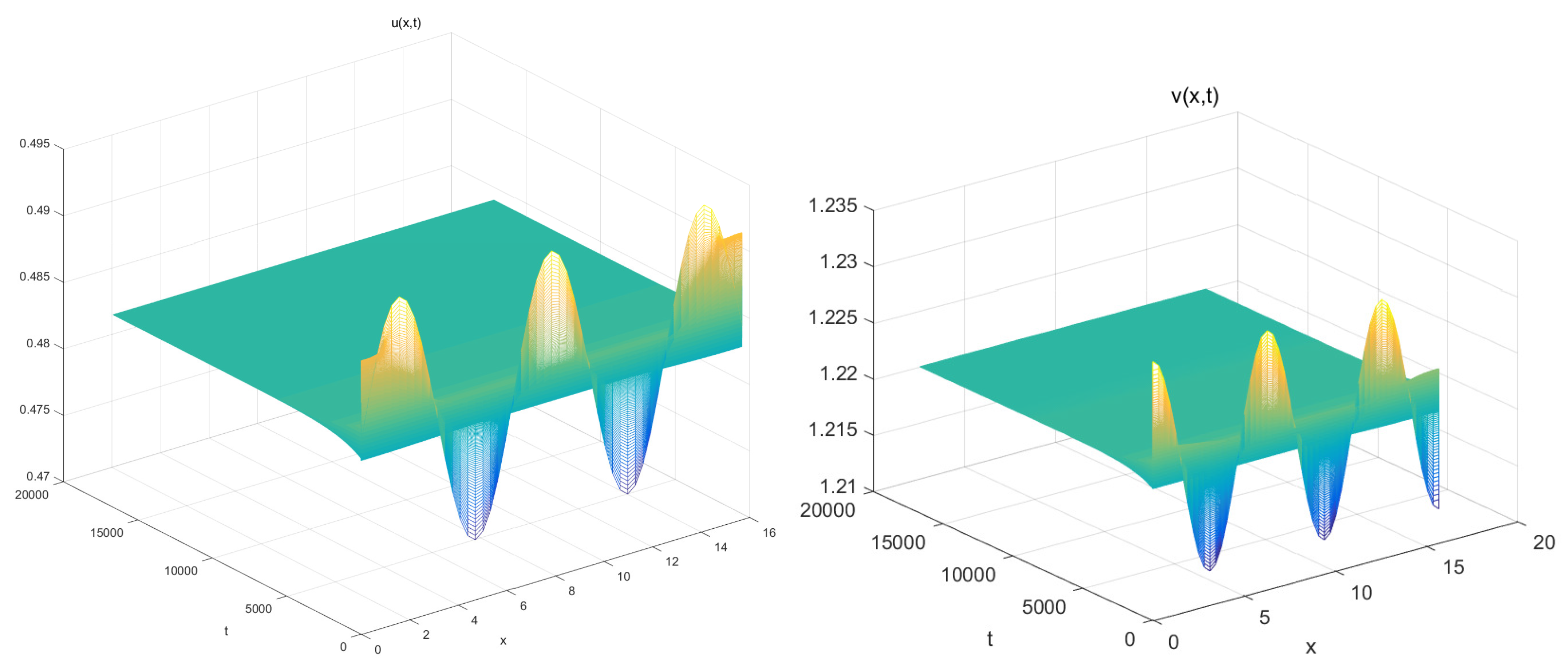
Hence, $\left(\mathbf{H}\right)$ holds. $\mathbb{G}=\{0,1\}\ne \varnothing$. Let $n=0$, then ${\tau }_{\ast }={\tau }_0^0\approx 0.8015$ and ${\omega }_0\approx 0.3771$ are obtained through calculation. From Theorem 1, $P(u_0,v_0)$ is stable for $\tau \in [0,{\tau }_{\ast })$. It is shown in Figure 1, here $\tau =0.5$. In Figure 1, we can see that the predator and prey coexist, and as time goes on, they tend to the positive equilibrium $(u_0,v_0)$. $P(u_0,v_0)$ is unstable and Hopf bifurcation occurs when $\tau ={\tau }_{\ast }$. From last section, we have $\xi \approx -0.9796i,$$\eta \approx -0.9232i.$ Next,

$$\begin{array}{c}\hfill {\mathsf{\Phi }}_1\left(0\right)=\left(\begin{array}{c}1\\ 0\end{array}\right),{\mathsf{\Phi }}_2\left(0\right)\approx \left(\begin{array}{c}0\\ -0.9796\end{array}\right),\end{array}$$

$$\begin{array}{cc}\hfill {\mathsf{\Psi }}_1^{\ast }\left(0\right)& =\left(\begin{array}{c}1\\ 0\end{array}\right),{\mathsf{\Psi }}_2^{\ast }\left(0\right)\approx \left(\begin{array}{c}0\\ -0.9232\end{array}\right).\hfill \end{array}$$

$n=0$, through (43), easily know

$$g_{20}\approx 0.1632+0.2342i,g_{11}\approx 0.0378-0.0672i,$$

$$g_{02}\approx -0.0876-0.3686i,g_{21}\approx -0.0341+0.1860i.$$

By Lemma 4 and its proof, we obtain

$$\frac{d\lambda }{d\tau }\approx 0.0079+0.0239i.$$

Finally, we can calculate the following parameters

$${\mu }_2\approx 1.7199>0,{\widehat{\beta }}_2\approx -0.0271<0,\mathrm{and}{T}_2\approx -0.2369<0.$$

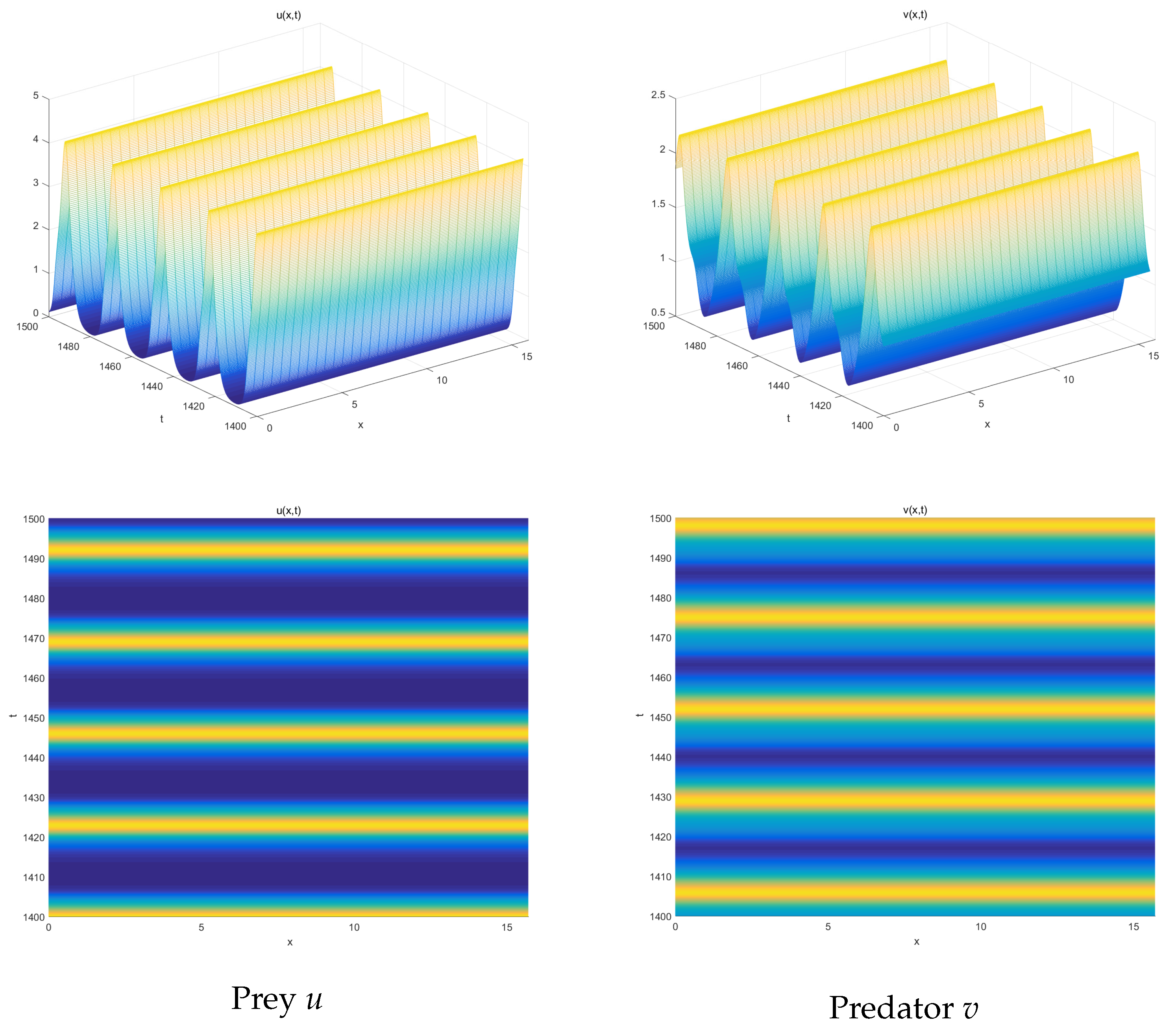
Thus, the direction of Hopf bifurcation is forward because ${\mu }_2>0$. There exists the locally asymptotically stable bifurcating periodic solutions whose period is decreasing (see Figure 2). At this moment, $\tau =1.3$, prey and predator will coexist in the form of periodic oscillation.

If we choose other parameters, Hopf bifurcation with period-2 can also occur. For the system (3), fix parameters

$$\begin{array}{cc}\hfill & d_1=2,d_2=2,\alpha =0.5,\beta =0.5,\gamma =4.1,\hfill \\ \hfill & \delta =0.4,w=0.3,ϵ=0.7,s=0.01,l=5.\hfill \end{array}$$

(52)

Then, we know $u_0\approx 0.4109$, $v_0\approx 1.2762$, and

$$a_1-\frac{u_0}{\gamma }\approx -0.0135<0,a_2{b}_1\approx -0.1141<0.$$

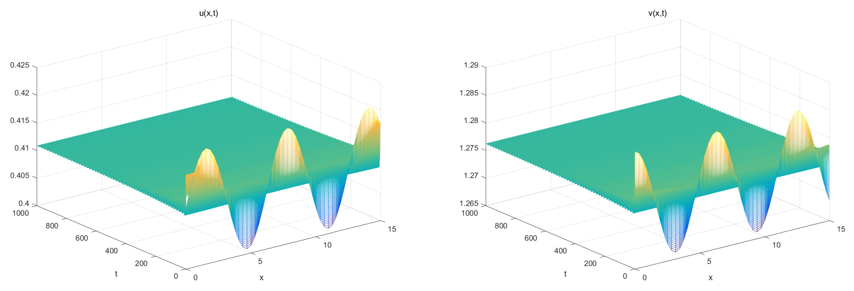
Hence, $\left(\mathbf{H}\right)$ holds. $\mathbb{G}=\{0,1\}\ne \varnothing$. Let $n=0$, ${\tau }_{\ast }={\tau }_0^0\approx 1.4414$ and ${\omega }_0\approx 0.3638$ are obtained through calculation. From Theorem 1, $P(u_0,v_0)$ is stable for $\tau \in [0,{\tau }_{\ast })$. It is shown in Figure 3, here $\tau =1$. In Figure 3, we can see that the predator and prey coexist, and as time goes on, they tend to the positive equilibrium $(u_0,v_0)$. $P(u_0,v_0)$ is unstable and Hopf bifurcation occurs when $\tau ={\tau }_{\ast }$. From last section, we have $\xi \approx -1.0825i,$$\eta \approx -0.7964i.$ Next,

$$\begin{array}{c}\hfill {\mathsf{\Phi }}_1\left(0\right)=\left(\begin{array}{c}1\\ 0\end{array}\right),{\mathsf{\Phi }}_2\left(0\right)=\left(\begin{array}{c}0\\ -1.0825\end{array}\right),\end{array}$$

$$\begin{array}{cc}\hfill {\mathsf{\Psi }}_1^{\ast }\left(0\right)& =\left(\begin{array}{c}1\\ 0\end{array}\right),{\mathsf{\Psi }}_2^{\ast }\left(0\right)=\left(\begin{array}{c}0\\ -0.7964\end{array}\right).\hfill \end{array}$$

$n=0$, through (43), we easily know that

$$g_{20}\approx 0.3125+0.5641i,g_{11}\approx 0.0668-0.0999i,$$

$$g_{02}\approx -0.1789-0.7639i,g_{21}\approx -0.3361-1.4048i.$$

By Lemma 4 and its proof, we obtain

$$\frac{d\lambda }{d\tau }\approx 0.0112+0.0177i.$$

Finally, we can calculate the following parameters:

$${\mu }_2\approx 15.4938>0,{\widehat{\beta }}_2\approx -0.3484<0,\mathrm{and}{T}_2\approx 1.1019>0.$$

Thus, the direction of Hopf bifurcation is forward because ${\mu }_2>0$. There exists the locally asymptotically stable bifurcating periodic solutions whose period is increasing (see Figure 4). At this moment, $\tau =1.5$, bifurcating periodic solutions with period-2 appears.

5. Conclusions

In this paper, we incorporated time delay and diffusion on the model (1), and studied the dynamics in a delayed diffusive system with anti-predator and additional food provided for a predator. By using time delay as a parameter, we mainly studied the local stability of coexisting equilibrium, the existence of Hopf bifurcation induced by delay, and the property of Hopf bifurcation by the theory of the center manifold and normal form method.

Compared with the model (1), we prove that under some conditions, time delay can destabilize the stable equilibrium, and can even lead to the existence of periodic solutions. Especially, there exists a critical value ${\tau }_{\ast }$. When the time delay is smaller than the critical value, prey and predator will coexist, and tend toward the coexisting equilibrium, and are evenly distributed homogeneous in the region; however, when the time delay crosses the critical value, the coexisting equilibrium is unstable, and Hopf bifurcation occurs. In this case, the prey and predator may also coexist, but they will coexist in the form of periodic oscillation. Further, diffusion may also cause inhomogeneous periodic solutions. Unfortunately, we found the inhomogeneous periodic solution of our model is unstable and could not be shown through numerical simulations. In a future work, we will conduct a more general study, using a generalized logistic function, which allows us to study the Allee effect. That is relevant in several areas of application, namely biology and ecology.

References

- Ford, J.K.; Reeves, R.R. Fight or flight: Antipredator strategies of baleen whales. Mamm. Rev. 2008, 38, 50–86. [Google Scholar] [CrossRef]
- Ge, D.; Chesters, D.; Gomez-Zurita, J. Anti-predator defence drives parallel morphological evolution in flea beetles. Proc. R. Soc. Lond. B Biol. Sci. 2011, 278, 2133–2141. [Google Scholar] [CrossRef] [PubMed] [Green Version]
- Lima, S.L. Nonlethal effectsin the ecology of predator-prey interactions. Bioscience 1998, 48, 25–34. [Google Scholar] [CrossRef] [Green Version]
- Matassa, C.M.; Donelan, S.C.; Luttbeg, B. Resource levels and prey state influence antipredator behavior and the strength of nonconsumptive predator effects. Oikos 2016, 125, 1478–1488. [Google Scholar] [CrossRef]
- Khater, M.; Murariu, D.; Gras, R. Predation risk tradeoffs in prey: Effects on energy and behaviour. Theor. Ecol. 2016, 9, 251–268. [Google Scholar] [CrossRef]
- Srinivasu, P.D.N.; Prasad, B.S.R.V.; Venkatesulu, M. Biological control through provision of additional food to predators: A theoretical study. Theor. Popul. Biol. 2007, 72, 111–120. [Google Scholar] [CrossRef] [PubMed]
- Prasad, K.D.; Prasad, B.S.R.V. Qualitative analysis of additional food provided predator-prey system with anti-predator behaviour in prey. Nonlinear Dyn. 2019, 96, 1765–1793. [Google Scholar] [CrossRef]
- Eskandari, Z.; Alidousti, J.; Avazzadeh, Z. Dynamics and bifurcations of a discrete-time prey-predator model with Allee effect on the prey population. Ecol. Complex. 2021, 48, 100962. [Google Scholar] [CrossRef]
- Zhang, X.; Liu, Z. Hopf bifurcation analysis in a predator-prey model with predator-age structure and predator-prey reaction time delay. Appl. Math. Model. 2021, 91, 530–548. [Google Scholar] [CrossRef]
- Duque, C.; Lizana, M. On the dynamics of a predator-prey model with nonconstant death rate and diffusion. Nonlinear Anal. Real World Appl. 2011, 12, 2198–2210. [Google Scholar] [CrossRef]
- Gan, Q.; Xu, R.; Yang, P. Bifurcation and chaos in a ratio-dependent predator-prey system with time delay. Chaos Solitons Fractals 2009, 39, 1883–1895. [Google Scholar] [CrossRef]
- Gilioli, G.; Pasquali, S.; Ruggeri, F. Nonlinear functional response parameter estimation in a stochastic predator-prey model. Math. Biosci. Eng. 2017, 9, 75–96. [Google Scholar]
- Wang, M. Stability and Hopf bifurcation for a prey-predator model with prey-stage structure and diffusion. Math. Biosci. 2008, 212, 149–160. [Google Scholar] [CrossRef] [PubMed]
- Guin, L.N.; Pal, S.; Chakravart, S. Pattern dynamics of a reaction-diffusion predator-prey system with both refuge and harvesting. Int. J. Biomath. 2021, 14, 2050084. [Google Scholar] [CrossRef]
- Djilali, S.; Bentout, S.; Ghanbari, B. Spatial patterns in a vegetation model with internal competition and feedback regulation. Eur. Phys. J. Plus 2021, 136, 1–24. [Google Scholar] [CrossRef]
- Souna, F.; Djilali, S.; Lakmeche, A. Spatiotemporal behavior in a predator–prey model with herd behavior and cross-diffusion and fear effect. Eur. Phys. J. Plus 2021, 136, 1–21. [Google Scholar] [CrossRef]
- Djilali, S.; Bentout, S. Pattern formations of a delayed diffusive predator–prey model with predator harvesting and prey social behavior. Math. Methods Appl. Sci. 2021, 44, 9128–9142. [Google Scholar] [CrossRef]
- Wu, J. Theory and Applications of Partial Functional Differential Equations; Springer: Berlin, Germany, 1996. [Google Scholar]
- Kreyszig, E. Introductory Functional Analysis with Applications; Wiley: New York, NY, USA, 1978; pp. 225–231. [Google Scholar]
- Hale, J. Theory of Functional Differential Equations; Springer: Berlin, Germany, 1977. [Google Scholar]
Figure 1.
The numerical simulations of system (3) with and other parameters is given by (51). Left: component u. Right: component v.
Figure 2.
The numerical simulations of system (3) with and other parameters is given by (51).
Figure 3.
The numerical simulations of system (3) with and other parameters is given by (52). Left: component u. Right: component v.
Figure 4.
The numerical simulations of system (3) with and other parameters is given by (52).