Painlevé Test and Exact Solutions for (1 + 1)-Dimensional Generalized Broer–Kaup Equations

Abstract

In this paper, the Painlevé integrable property of the (1 + 1)-dimensional generalized Broer–Kaup (gBK) equations is first proven. Then, the Bäcklund transformations for the gBK equations are derived by using the Painlevé truncation. Based on a special case of the derived Bäcklund transformations, the gBK equations are linearized into the heat conduction equation. Inspired by the derived Bäcklund transformations, the gBK equations are reduced into the Burgers equation. Starting from the linear heat conduction equation, two forms of N-soliton solutions and rational solutions with a singularity condition of the gBK equations are constructed. In addition, the rational solutions with two singularity conditions of the gBK equation are obtained by considering the non-uniqueness and generality of a resonance function embedded into the Painlevé test. In order to understand the nonlinear dynamic evolution dominated by the gBK equations, some of the obtained exact solutions, including one-soliton solutions, two-soliton solutions, three-soliton solutions, and two pairs of rational solutions, are shown by three-dimensional images. This paper shows that when the Painlevé test deals with the coupled nonlinear equations, the highest negative power of the coupled variables should be comprehensively considered in the leading term analysis rather than the formal balance between the highest-order derivative term and the highest-order nonlinear term.

1. Introduction

Painlevé analysis is an important method for testing Painlevé integrable property [1,2,3,4,5,6,7] of nonlinear partial differential equations (PDEs). If a given nonlinear PDE passes through the Painlevé test, then we say it has Painlevé property [1]. More specifically, Painlevé property or Painlevé integrability for nonlinear PDEs means that the solutions of the given PDE must be “single-valued” in the neighborhood of a movable singularity manifold (non-characteristic). The so-called WTC method of Painlevé analysis proposed by Weiss, Tabor, and Carnevale [2] is an effective approach for Painlevé test of nonlinear PDEs. As pointed out in [4], the celebrated BK equations can be used to describe the propagation with double directions of long waves located in shallow water. In 2013, Zhang, Han, and Tam [8] derived the following (1 + 1)-dimensional gBK equations:

$$v_t=v_{xx}-2v{v}_x-4w_x$$

(1)

$$w_t=-w_{xx}-2{(wv)}_x-2v_x$$

(2)

In soliton theory, besides the Painlevé analysis method [1,2,3], there are many alternative methods [9,10,11,12,13,14,15,16,17] for solving nonlinear PDEs. Generally, each of these methods has its advantages and disadvantages. Both the inverse scattering method [9] and the Darboux transformation [11] depends on the Lax pair of the solved equations; however, constructing the Lax pair sometimes is more difficult than solving the equation itself or even impossible. One of the key steps of the Hirota’s bilinear method [10] is finding an effective dependent variable transformation, which is often inseparable from attempts or known solutions. Most of other methods, such as [12,13,14,15,16], are relatively direct, but the hypothetical forms of ansatz solution limit the type of the constructing solutions. The Painlevé analysis method [1,2,3] can give the relative unified form of the solution of the equation to the greatest extent and can construct various formal solutions from this unified form as needed. It is worth mentioning that one of the advantages of the Painlevé analysis method [1,2,3] is to provide a useful tool for the reduction or linearization of nonlinear PDEs. The Lax integrability and multiple soliton solutions of Equations (1) and (2) were obtained in [8,18,19]. As far as we know, the Painlevé test of Equations (1) and (2) has not been reported. In this paper, we extend the WTC method [2] to prove the Painlevé property of Equations (1) and (2). At the same time, the Bäcklund transformations, two reductions, and some exact solutions of Equations (1) and (2) have been obtained by using the Painlevé truncation technique. This is due to our consideration of balancing $v_{xx}-4w_x$ and $2v{v}_x$ rather than the highest-order derivative term $v_{xx}$ and the highest-order nonlinear term $2v{v}_x$ in form for Equation (1) in the process of using the Painlevé test to deal with the leading term analysis.

2. Painlevé Test and Painlevé Integrability

Employing the WTC method [2] of Painlevé analysis, we suppose that

$$v={\varphi }^{-\alpha }{\displaystyle \sum _{j=0}^{\infty }{v}_j{\varphi }^j}, v_0\ne 0,$$

(3)

$$w={\varphi }^{-\beta }{\displaystyle \sum _{j=0}^{\infty }{w}_j{\varphi }^j}, w_0\ne 0,$$

(4)

where $\varphi$, $v_j$, and $w_j$ are functions of $x$ and $t$, $\alpha$, and $\beta$ are non-negative integers. Considering the leading term analysis, we take

$$v\sim v_0{\varphi }^{-\alpha }$$

(5)

$$w\sim w_0{\varphi }^{-\beta }$$

(6)

and therefore have

$$v_x\sim -\alpha v_0{\varphi }^{-\alpha -1}{\varphi }_x, v_{xx}\sim \alpha (\alpha +1)v_0{\varphi }^{-\alpha -2}{\varphi }_x^2,$$

(7)

$$w_x\sim -\beta w_0{\varphi }^{-\beta -1}{\varphi }_x, w_{xx}\sim \beta (\beta +1)w_0{\varphi }^{-\beta -2}{\varphi }_x^2.$$

(8)

Using Equations (5)–(8) to balance the following terms of Equations (1) and (2),

$$v_{xx}-2v{v}_x-4w_x=0,$$

(9)

$$-w_{xx}-2{(wv)}_x=0,$$

(10)

We arrive at

$$\alpha =1, v_0={\varphi }_x,$$

(11)

$$\beta =2, w_0=-\frac{1}{2}{\varphi }_x^2.$$

(12)

Thus, Equations (3) and (4) can be rewritten as

$$v={\displaystyle \sum _{j=0}^{\infty }{v}_j{\varphi }^{j-1}},$$

(13)

$$w={\displaystyle \sum _{j=0}^{\infty }{w}_j{\varphi }^{j-2}}.$$

(14)

Substituting Equations (13) and (14) into Equations (1) and (2), collecting the same power coefficients of $\varphi$, and then setting all the coefficients as zeros, we have

$${\varphi }^{-3}:2{\varphi }_x(v_0^2+4w_0+v_0{\varphi }_x)=0,$$

(15)

$${\varphi }^{-2}:4w_1{\varphi }_x-2{\varphi }_x{v}_{0,x}-4w_{0,x}+v_0({\varphi }_t+2v_1{\varphi }_x-2v_{0,x}-{\varphi }_{xx})=0,$$

(16)

$${\varphi }^{j-1}:v_{j+2}[j(j+1){\varphi }_x^2-2j{v}_0{\varphi }_x]-4j{w}_{j+2}{\varphi }_x=F_{j+2,1}, (j=0,1,2,\cdots ),$$

(17)

$${\varphi }^{-4}:6w_0{\varphi }_x(v_0-{\varphi }_x)=0,$$

(18)

$${\varphi }^{-3}:2[v_0(2w_1{\varphi }_x-w_{0,x})+{\varphi }_x(-w_1{\varphi }_x+2w_{0,x})+w_0({\varphi }_t+2v_1{\varphi }_x-v_{0,x}+{\varphi }_{xx})]=0,$$

(19)

$${\varphi }^{j-2}:v_{j+2}[-2(j-1)w_0{\varphi }_x]-2(j-1)w_{j+2}(j{\varphi }_x^2+v_0{\varphi }_x)=F_{j+2,2}, (j=0,1,2,\cdots ),$$

(20)

where $F_{j+2,1}$ and $F_{j+2,2}$ are functions of $v_0$, $w_0$, $v_1$, $w_1$, $v_2$, $w_2$, $\cdots$,$v_{j+1}$, $w_{j+1}$, $\varphi$ and their partial derivatives with respect to $x$ and $t$. It is easy to see that Equations (15) and (18) give the same $v_0$ and $w_0$ as Equations (11) and (12). From Equation (16), one has

$$v_1=-\frac{{\varphi }_t+{\varphi }_{xx}}{2{\varphi }_x}, w_1=\frac{1}{2}{\varphi }_{xx}.$$

(21)

In view of Equations (11), (12), (17), and (20), we drive the determinants of the coefficients of $v_j$ and $w_j$$(j=2,3,4,\cdots )$

$$\left|\begin{array}{cc}(j-2)(j-3){\varphi }_x^2& -4(j-2){\varphi }_x\\ (j-3){\varphi }_x^3& -2(j-3)(j-1){\varphi }_x^2\end{array}\right|=-2(j-2)(j-3)(j^2-4j+1){\varphi }_x^4.$$

(22)

Equation (22) hints that $j=2,3$ are the resonance points. Accordingly, $v_2$ and $w_3$ or $v_3$ and $w_2$ may be the corresponding resonance functions. Fortunately, when we select $v_2$ and $w_3$ as the resonance functions and set $v_2=0$ and $w_3=0$, Equation (20) gives

$$w_2=\frac{{\varphi }_{xx}({\varphi }_t+{\varphi }_{xx})-{\varphi }_x(4{\varphi }_x+{\varphi }_{xt}+{\varphi }_{xxx})}{4{\varphi }_x^2}.$$

(23)

Further set $v_j=0(j\ge 3)$ and $w_j=0(j\ge 4)$; then, Equations (3) and (4) can be truncated. This shows that the (1 + 1)-dimensional gBK Equations (1) and (2) pass the Painlevé test and hence possess the Painlevé integrability.

3. Bäcklund Transformations and Two Reductions

For the (1 + 1)-dimensional gBK Equations (1) and (2), the following Bäcklund transformations hold:

Theorem 1.

The (1 + 1)-dimensional gBK Equations (1) and (2) have the Bäcklund transformations:

$$v=\frac{{\varphi }_x}{\varphi }+v_1$$

(24)

$$w=-\frac{{\varphi }_x^2}{2{\varphi }^2}+\frac{{\varphi }_{xx}}{2\varphi }+\frac{1}{2}{v}_{1,x}-1,$$

(25)

where$\varphi$and$v_1$satisfy the following equations:

$${\varphi }_t+2v_1{\varphi }_x+{\varphi }_{xx}=0,$$

(26)

$$v_{1,t}+2v_1{v}_{1,x}+v_{1,xx}=0.$$

(27)

Proof of Theorem 1.

Setting $v_j=0(j\ge 2)$ and $w_j=0(j\ge 3)$, we can truncate Equations (3) and (4) as

$$v=v_0{\varphi }^{-1}+v_1$$

(28)

$$w=w_0{\varphi }^{-2}+w_1{\varphi }^{-1}+w_2$$

(29)

Substituting Equations (28) and (29), together with $v_0$, $w_0$, and $w_1$ in Equations (11), (12), and (21) into Equations (1) and (2), then collecting the same power coefficients of $\varphi$ and setting all the coefficients as zeros, we can arrive at Equation (26). At the same time, with the help of Equation (26), we have

$$v_{1,t}+2v_1{v}_{1,x}+4w_{2,x}-v_{1,xx}=0$$

(30)

$$w_2=\frac{1}{2}{v}_{1,x}-1.$$

(31)

Inserting Equation (31) into Equation (30), we reach Equation (27). Using Equations (11), (12), (21), and (31), we finally convert Equations (28) and (29) into Equations (24) and (25). □

Corollary 1.

Under the transformations:

$$v=\frac{{\varphi }_x}{\varphi }$$

(32)

$$w=-\frac{{\varphi }_x^2}{2{\varphi }^2}+\frac{{\varphi }_{xx}}{2\varphi }-1,$$

(33)

the (1 + 1)-dimensional gBK Equations (1) and (2) can be reduced to the linear heat conduction equation:

$${\varphi }_t+{\varphi }_{xx}=0$$

(34)

Proof of Corollary 1.

Obviously, when $v_1=0$, Equations (26) and (27) degenerate into Equation (34). Meanwhile, Equations (24) and (25) become Equations (32) and (33). □

Inspired by Equation (27) derived from the substitution of Equations (31) into Equation (30), we get the following Theorem 2.

Theorem 2.

Suppose that

$$w=\frac{1}{2}{v}_x-1$$

(35)

the (1 + 1)-dimensional gBK Equations (1) and (2) can be reduced to the Burgers equation:

$$v_t+2v{v}_x+v_{xx}=0$$

(36)

Proof of Theorem 2.

On the one hand, we can reduce Equation (1) into Equation (36) by using Equation (35). On the other hand, the substitution of Equation (35) into Equation (2) gives

$${(v_t+2v{v}_x+v_{xx})}_x=0$$

(37)

Since when Equation (36) is true, Equation (37) naturally holds, we then conclude that Equation (35) can transform Equations (1) and (2) into Equation (36). □

4. Soliton Solutions and Rational Solutions

To construct exact solutions of the (1 + 1)-dimensional gBK Equations (1) and (2), we consider Equations (32)–(34) and suppose that

$$\varphi =1+e^{k_1(x+c_{1}t+d_1)}$$

(38)

where $k_1$, $c_1$, and $d_1$ are constants. Then, Equation (34) dictates

$$c_1=-k_1$$

(39)

Thus, we obtain one-soliton solutions of Equations (1) and (2):

$$v=\frac{k_1{e}^{k_1(x-k_{1}t+d_1)}}{1+e^{k_1(x-k_{1}t+d_1)}}$$

(40)

$$w=-\frac{k_1^2{e}^{2k_1(x-k_{1}t+d_1)}}{2{(1+e^{k_1(x-k_{1}t+d_1)})}^2}+\frac{k_1^2{e}^{k_1(x-k_{1}t+d_1)}}{2(1+e^{k_1(x-k_{1}t+d_1)})}-1.$$

(41)

Considering the linearity of Equation (34), we know that

$$\varphi =1+{\displaystyle \sum _{i=1}^N{e}^{k_i(x-k_{i}t+d_i)}}, c_i=-k_i(i=1,2,\cdots ,N)$$

(42)

still solves Equation (34). Thus, we obtain N-soliton solutions of Equations (1) and (2):

$$v=\frac{{\displaystyle \sum _{i=1}^N{k}_i{e}^{k_i(x-k_{i}t+d_i)}}}{1+{\displaystyle \sum _{i=1}^N{e}^{k_i(x-k_{i}t+d_i)}}}={\left[\ln \left(1+{\displaystyle \sum _{i=1}^N{e}^{k_i(x-k_{i}t+d_i)}}\right)\right]}_x,$$

(43)

$$w=-\frac{{\left({\displaystyle \sum _{i=1}^N{k}_i{e}^{k_i(x-k_{i}t+d_i)}}\right)}^2}{2{\left(1+{\displaystyle \sum _{i=1}^N{e}^{k_i(x-k_{i}t+d_i)}}\right)}^2}+\frac{{\displaystyle \sum _{i=1}^N{k}_i^2{e}^{k_i(x-k_{i}t+d_i)}}}{2\left(1+{\displaystyle \sum _{i=1}^N{e}^{k_i(x-k_{i}t+d_i)}}\right)}-1=\frac{1}{2}{\left[\ln \left(1+{\displaystyle \sum _{i=1}^N{e}^{k_i(x-k_{i}t+d_i)}}\right)\right]}_{xx}-1$$

(44)

We note here that the more general N-soliton solutions,

$$v={\left\{\ln \left[\left(1+{\displaystyle \sum _{i=1}^N{e}^{k_{i}x+k_i(2A-k_i)t+{\xi }_i^0}}\right)/e^{A(x+At)+{\eta }^0}\right]\right\}}_x,$$

(45)

$$w=\frac{1}{2}{\left\{\ln \left[\left(1+{\displaystyle \sum _{i=1}^N{e}^{k_{i}x+k_i(2A-k_i)t+{\xi }_i^0}}\right)e^{A(x+At)+{\eta }^0}\right]\right\}}_{xx}-1,$$

(46)

which include Equations (43) and (44) as special cases, have been obtained in our previous work [19]. In order to construct other formal N-soliton solutions of Equations (1) and (2), we assume that

$$\varphi =\left(1+{\displaystyle \sum _{i=1}^N{e}^{k_i(x+c_{i}t+d_i)}}\right)e^{p(x+qt+r)},$$

(47)

where $k_i$, $c_i$, $d_i$, $p$, $q$, and $r$ are all constants. Then, the substitution of Equation (47) into Equation (34) determines the relations:

$$c_i=-k_i-2p, q=-p.$$

(48)

We therefore gain the formal N-soliton solutions of Equations (1) and (2):

$$v=\ln {\left[\left(1+{\displaystyle \sum _{i=1}^N{e}^{k_i[x-(k_i-2p)t+d_i]}}\right)e^{p(x-pt+r)}\right]}_x,$$

(49)

$$w=\frac{1}{2}{\left\{\ln \left[\left(1+{\displaystyle \sum _{i=1}^N{e}^{k_i[x-(k_i-2p)t+d_i]}}\right)e^{p(x-pt+r)}\right]\right\}}_{xx}-1.$$

(50)

Here, it should be noted when Equation (50) is equivalent to Equation (46), then Equation (49) is different from Equation (45). Besides, we easily see that Equations (43) and (44) are special cases of Equations (49) and (50). The equivalent forms of Equations (49) and (50) are also helpful for the comparison, which reads

$$v=\frac{{\displaystyle \sum _{i=1}^N{k}_i{e}^{k_i[x-(k_i-2p)t+d_i]}}}{1+{\displaystyle \sum _{i=1}^N{e}^{k_i[x-(k_i-2p)t+d_i]}}}+p$$

(51)

$$w=-\frac{{\left[{\displaystyle \sum _{i=1}^N{k}_i{e}^{k_i[x-(k_i-2p)t+d_i]}}\right]}^2}{2{\left[1+{\displaystyle \sum _{i=1}^N{e}^{k_i[x-(k_i-2p)t+d_i]}}\right]}^2}+\frac{{\displaystyle \sum _{i=1}^N{k}_i^2{e}^{k_i[x-(k_i-2p)t+d_i]}}}{2\left[1+{\displaystyle \sum _{i=1}^N{e}^{k_i[x-(k_i-2p)t+d_i]}}\right]}-1.$$

(52)

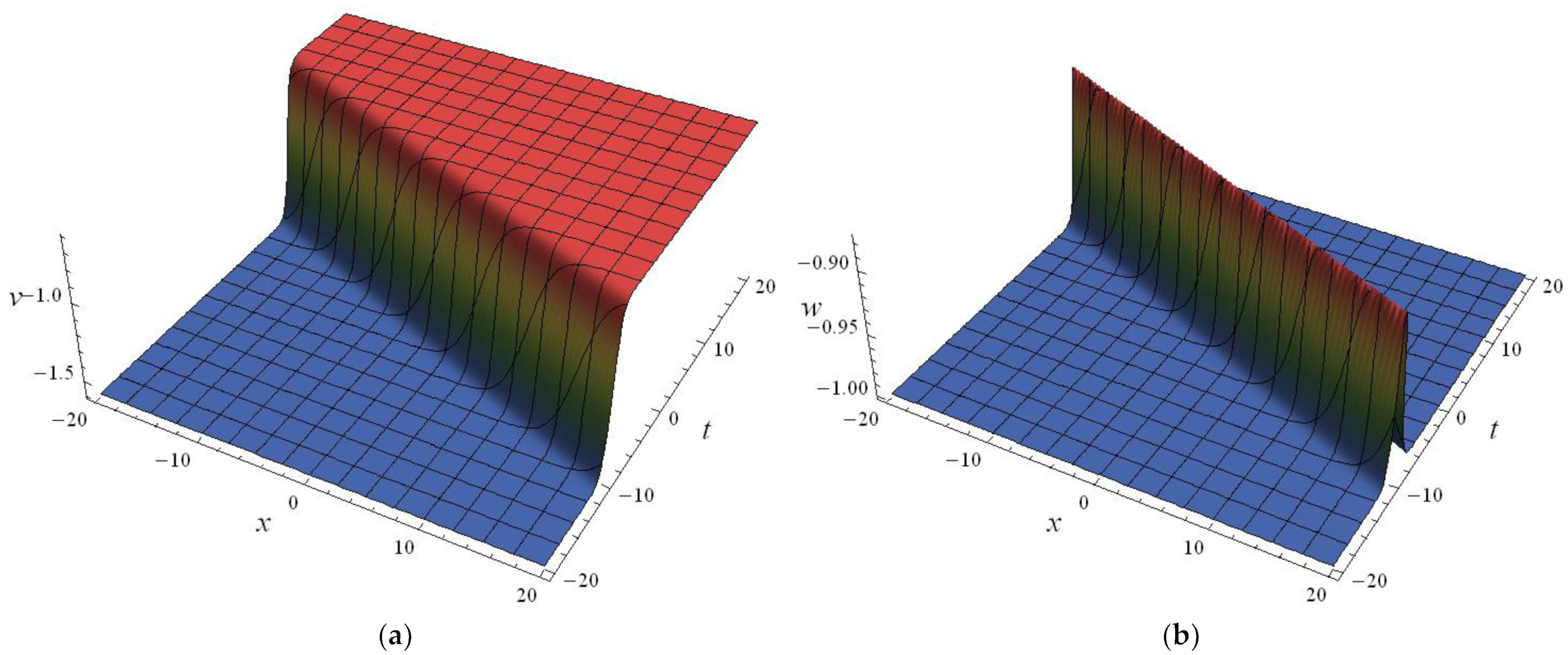
In Figure 1, the one-soliton solutions determined by Equations (51) and (52) are shown by setting $k_1=-1$, $d_1=0$, and $p=-0.6$. It can be seen from Figure 1 that the one-soliton solution determined by Equation (51) possesses kink structure, and the one-soliton solution determined by Equation (52) has bell structure.

The head-on two kink-soliton solution and the head-on two bell-soliton solution determined by Equations (51) and (52) are shown in Figure 2 by setting $k_1=1$, $k_2=-1.1$, $d_1=0$, $d_2=0$, and $p=-0.6$.

The interaction of three kink-soliton solution determined by Equation (51) and the interaction of three bell-soliton solution determined by Equation (52) are shown in Figure 3; there, the parameters are selected as $k_1=-1$, $k_2=-1.5$, $k_3=0.8$, $d_1=0$, $d_2=0$, $d_3=0$, and $p=-0.6$.

In addition to the soliton solutions obtained above, some other types of exact solutions of Equations (1) and (2) can also be obtained. For example, if we choose Equation (26) in the form

$$\varphi =k(x-ct)+d$$

(53)

where $k$, $c$, and $d$ are all constants, then one has

$$v_0=k, v_1=\frac{1}{2}c, w_0=-\frac{1}{2}{k}^2, w_1=0, w_2=-1.$$

(54)

The rational solutions of Equations (1) and (2) are then obtained as follows:

$$v=\frac{k}{k(x-ct)+d}+\frac{1}{2}c,$$

(55)

$$w=-\frac{k^2}{2{[k(x-ct)+d]}^2}-1.$$

(56)

In Figure 4, the rational solutions (55) and (56) are shown by selecting $c=1$, $k=-2$, and $d=3$. A direct computation shows that the singularities in Figure 4 occur at each point on the straight line $2(x-t)-3=0$.

The above results obtained benefit from the correct selection of the resonance coefficient functions for $v_2$ and $w_3$ in Equations (17) and (20). In fact, if we keep the generality of $v_2$, the equation $v_2{v}_{2,x}=0$ will appear in the operation of the above Painlevé test. When $v_2=0$ is selected, then the rational solutions (55) and (56) can be obtained by employing Equation (53). To avoid repetition, we omit them here. However, when we select $v_{2,x}=0$ together with Equation (53), the similar operations give

$$v_2=\frac{1}{2kt-s}$$

(57)

where $s$ is an arbitrary constant and hence produces the general rational solutions of Equations (1) and (2):

$$v=\frac{k}{k(x-ct)+d}+\frac{k(x-ct)+d}{2kt-s}+\frac{1}{2}c$$

(58)

$$w=-\frac{k^2}{2{[k(x-ct)+d]}^2}+\frac{k}{2(2kt-s)}-1$$

(59)

which causes singularities to occur in two straight lines, $k(x-ct)+d=0$ and $2kt-s=0$, in the case of $k\ne 0$. See Figure 5 for the rational solutions (58) and (59) with the parameters $c=1$, $k=-2$, $d=3$, and $s=-2$.

5. Conclusions

We have proved the Painlevé integrable property of the (1 + 1)-dimensional gBK Equations (1) and (2). This is due to the key step adopted in this paper to balance Equations (9) and (10) rather than the equation

$$v_{xx}-2v{v}_x=0$$

(60)

and Equation (10) in the process of using the Painlevé test to deal with the leading term analysis. If the leading terms of Equations (60) and (10) are balanced, then $\alpha =1$ and $v_0=-{\varphi }_x$ are derived from Equation (60) by similar computations using Equations (5) and (6). Substituting $\alpha =1$ and $v_0=-{\varphi }_x$ into Equation (10) and balancing the leading terms yields $\beta =-1$ or $\beta =-2$. This contradicts the prior assumption that $\beta$ is a nonnegative integer. Although the derivative of $v_{xx}$ is one order higher than that of $w_x$ in form, the highest negative power of $\varphi$ is balanced, and $v_{xx}\sim 2v_0{\varphi }_x^2{\varphi }^{-3}$ and $w_x\sim -2w_0{\varphi }_x{\varphi }^{-3}$ are the same power as discussed in this paper. For other coupled nonlinear PDEs, this should be noted in the leading term analysis. Of course, this noteworthy point will not appear in a single model. We think this point is very important and will directly affect whether the Painlevé test can be passed if the equation under consideration has Painlevé property. To the best of our knowledge, it has not been reported in the literature.

Based on the Painlevé truncation, the Bäcklund transformations (24)–(27) and exact solutions of Equations (1) and (2) have been obtained, including the N-soliton solutions (43) and (44), (49) and (50), rational solutions (55) and (56), and (58) and (59). These obtained soliton solutions and rational solutions may provide useful information for explaining some relevant nonlinear physical phenomena. This shows the importance of the Bäcklund transformations (24)–(27) in constructing exact solutions to a great extent. Using the Bäcklund transformations (24)–(27) to construct other types of exact solutions of Equations (1) and (2) is worthy of study. Besides, the gBK Equations (1) and (2) are reduced into two simple forms by the aid of the benefits of the Bäcklund transformations (24)–(27). One reduced form gives the linear heat conduction Equation (34), and the other ones arrive at the Burgers Equation (36). Compared with the bilinear forms (2.8a) and (2.8b) [19], which are nonlinear, of Equations (1) and (2), the linear heat conduction Equation (34) in this paper is much simpler. Based on the bilinear forms (2.8a) and (2.8b) [19], the perturbation truncation technique of the Hirtoa’s bilinear method [10] can obtain the truncated expansion with any finite terms consisting of the solutions to construct. However, the Painlevé truncation, as did in this paper for Equations (1) and (2), will generally stop at the resonance point, and the number of expansion terms of the solution is small. It is difficult for the Painlevé analysis method [1,2,3] to construct the formal solutions of Equations (1) and (2) with any number of expansion terms, and the convergence of the infinite term series expansion solution (3) or (4) is far from being solved.

References

- Ablowitz, M.J.; Clarkson, P.A. Solitons, Nonlinear Evolution Equations and Inverse Scattering; Cambridge University Press: New York, NY, USA, 1991. [Google Scholar]
- Weiss, J.; Tabor, M.; Carnvale, C. The Painlevé property for partial differential equations. J. Math. Phys. 1983, 24, 522–526. [Google Scholar] [CrossRef]
- Kruskal, M.D.; Joshi, N.; Halburd, R. Analytic and asymptotic methods for nonlinear singularity analysis: A review and extensions of tests for the Painlevé property. Lect. Notes Phys. 1997, 495, 171–205. [Google Scholar]
- Zhang, S.L.; Wu, B.; Lou, S.Y. Painlevé analysis and special solutions of generalized Broer-Kaup equations. Phys. Lett. A 2002, 300, 40–48. [Google Scholar] [CrossRef]
- Kumar, S.; Singh, K.; Gupta, R.K. Painlevé analysis, Lie symmetries and exact solutions for (2+1)-dimensional variable coefficients Broer-Kaup equations. Commun. Nonlinear Sci. Numer. Simulat. 2012, 17, 1529–1541. [Google Scholar] [CrossRef]
- Zhang, S.; Chen, M.T.; Qian, W.Y. Painleve analysis for a forced Korteveg-de Vries equation arisen in fluid dynamics of internal solitary waves. Therm. Sci. 2015, 19, 1223–1226. [Google Scholar] [CrossRef]
- Zhang, S.; Chen, M.T. Painlevé integrability and new exact solutions of the (4+1)-dimensional Fokas equation. Math. Probl. Engin. 2015, 2015, 367425. [Google Scholar] [CrossRef] [Green Version]
- Zhang, Y.F.; Han, Z.; Tam, H.W. An integrable hierarchy and Darboux transformations, bilinear Bäcklund transformations of a reduced equation. Appl. Math. Comput. 2013, 219, 5837–5848. [Google Scholar] [CrossRef]
- Gardner, C.S.; Greene, J.M.; Kruskal, M.D.; Miura, R.M. Method for solving the Korteweg-de Vries equation. Phys. Rev. Lett. 1967, 19, 1095–1197. [Google Scholar] [CrossRef]
- Hirota, R. Exact envelope-soliton solutions of a nonlinear wave equation. J. Math. Phys. 1973, 14, 805–809. [Google Scholar] [CrossRef]
- Matveev, V.B.; Salle, M.A. Darboux Transformation and Soliton; Springer: Berlin/Heidelberg, Germany, 1991. [Google Scholar]
- Wang, M.L. Exact solutions for a compound KdV-Burgers equation. Phys. Lett. A 1996, 213, 279–287. [Google Scholar] [CrossRef]
- Fan, E.G. Travelling wave solutions in terms of special functions for nonlinear coupled evolution systems. Phys. Lett. A 2002, 300, 243–249. [Google Scholar] [CrossRef]
- He, J.H.; Wu, X.H. Exp-function method for nonlinear wave equations. Chaos Soliton. Fract. 2006, 30, 700–708. [Google Scholar] [CrossRef]
- Zhang, S.; Xia, T.C. A generalized auxiliary equation method and its application to (2+1)-dimensional asymmetric Nizhnik-Novikov-Vesselov equations. Phys. A Math. Theor. 2007, 40, 227. [Google Scholar] [CrossRef]
- Ma, W.X.; Lee, J.H. A transformed rational function method and exact solutions to 3+1 dimensional Jimbo-Miwa equation. Chaos Soliton. Fract. 2009, 42, 1356–1363. [Google Scholar] [CrossRef] [Green Version]
- Tian, S.F.; Zhang, H.Q. Riemann theta functions periodic wave solutions and rational characteristics for the (1 + 1)-dimensional and (2 + 1)-dimensional Ito equation. Chaos Soliton. Fract. 2013, 47, 27–41. [Google Scholar] [CrossRef]
- Zhang, S.; Liu, D.D. The third kind of Darboux transformation and multisoliton solutions for generalized Broer-Kaup equations. Turk. J. Phys. 2015, 39, 165–177. [Google Scholar] [CrossRef]
- Zhang, S.; Zheng, X.W. N-soliton solutions and nonlinear dynamics for two generalized Broer-Kaup systems. Nonlinear Dyn. 2022, 107, 1179–1193. [Google Scholar] [CrossRef]
Figure 1.
One-soliton solutions determined by Equations (51) and (52) with the parameters , , and : (a) One kink-soliton solution; (b) one bell-soliton solution.
Figure 2.
Two-soliton solutions determined by Equations (51) and (52) with the parameters , , , , and : (a) Two kink-soliton solution; (b) two bell-soliton solution.
Figure 3.
Three-soliton solutions determined by Equations (51) and (52) with the parameters , , , , , , and : (a) Kink three-soliton solution; (b) bell three-soliton solution.
Figure 4.
Rational solutions (55) and (56) with the parameters , , and : (a) Rational solution (55); (b) rational solution (56).
Figure 5.
Rational solutions (58) and (59) with the parameters , , , and : (a) Rational solution (58); (b) rational solution (59).
Publisher’s Note: MDPI stays neutral with regard to jurisdictional claims in published maps and institutional affiliations. |
© 2022 by the authors. Licensee MDPI, Basel, Switzerland. This article is an open access article distributed under the terms and conditions of the Creative Commons Attribution (CC BY) license (https://creativecommons.org/licenses/by/4.0/).
Share and Cite
MDPI and ACS Style
Zhang, S.; Xu, B. Painlevé Test and Exact Solutions for (1 + 1)-Dimensional Generalized Broer–Kaup Equations. Mathematics 2022, 10, 486. https://0-doi-org.brum.beds.ac.uk/10.3390/math10030486
AMA Style
Zhang S, Xu B. Painlevé Test and Exact Solutions for (1 + 1)-Dimensional Generalized Broer–Kaup Equations. Mathematics. 2022; 10(3):486. https://0-doi-org.brum.beds.ac.uk/10.3390/math10030486
Chicago/Turabian StyleZhang, Sheng, and Bo Xu. 2022. "Painlevé Test and Exact Solutions for (1 + 1)-Dimensional Generalized Broer–Kaup Equations" Mathematics 10, no. 3: 486. https://0-doi-org.brum.beds.ac.uk/10.3390/math10030486
Note that from the first issue of 2016, this journal uses article numbers instead of page numbers. See further details here.