
Multiscale Balanced-Attention Interactive Network for Salient Object Detection


1
Electronic Information School, Wuhan University, Wuhan 430072, China
2
School of Information and Communication, Guilin University of Electronic Technology, Guilin 541004, China
*
Authors to whom correspondence should be addressed.
Mathematics 2022, 10(3), 512; https://0-doi-org.brum.beds.ac.uk/10.3390/math10030512
Submission received: 28 December 2021
/
Revised: 28 January 2022
/
Accepted: 30 January 2022
/
Published: 5 February 2022
(This article belongs to the Special Issue Advances of Data-Driven Science in Artificial Intelligence)
Abstract
:The purpose of saliency detection is to detect significant regions in the image. Great progress on salient object detection has been made using from deep-learning frameworks. How to effectively extract and integrate multiscale information with different depths is an open problem for salient object detection. In this paper, we propose a processing mechanism based on a balanced attention module and interactive residual module. The mechanism addressed the acquisition of the multiscale features by capturing shallow and deep context information. For effective information fusion, a modified bi-directional propagation strategy was adopted. Finally, we used the fused multiscale information to predict saliency features, which were combined to generate the final saliency maps. The experimental results on five benchmark datasets show that the method is on a par with the state of the art for image saliency datasets, especially on the PASCAL-S datasets, where the MAE reaches 0.092, and on the DUT-OMROM datasets, where the F-measure reaches 0.763.
1. Introduction and Background
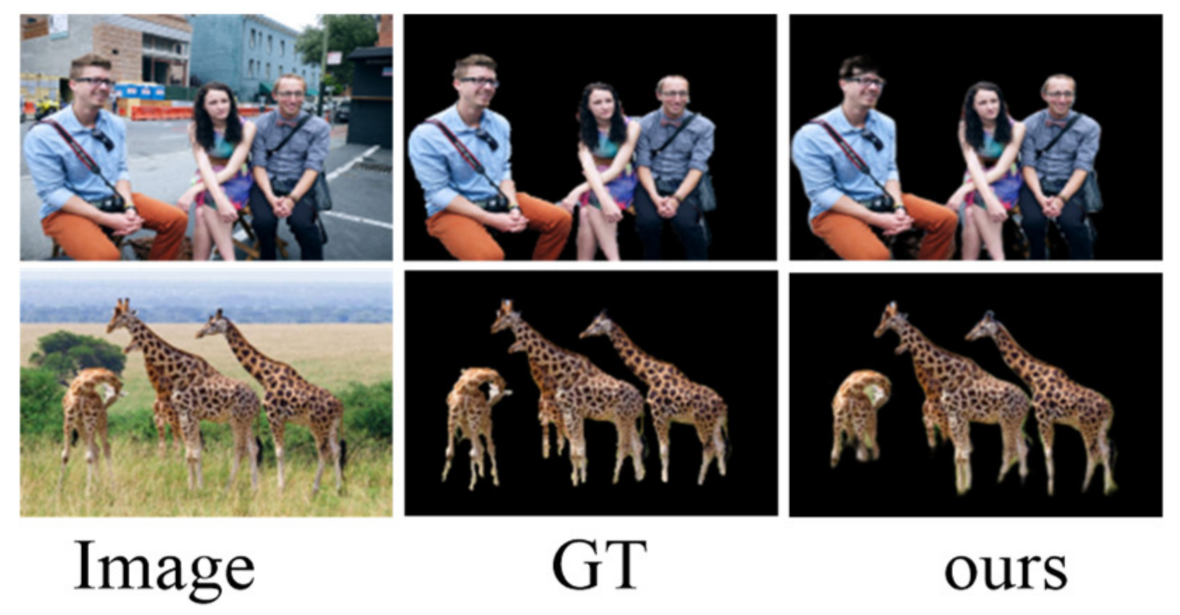
Salient object detection (SOD) aims to localize the most visually obvious regions in an image. SOD has been used in many computer-vision tasks, such as image retrieval [1,2], visual tracking [3], scene segmentation [4], object recognition [5], image contrast enhancement [6], assisted medicine [7,8,9], etc. Meanwhile, the specific scenarios of salient object detection in mobile communications applications, such as image background filtering and background atomization in mobile applications, all rely on the high accuracy of foreground target extraction, as shown in Figure 1. Scholars have also proposed many models [10,11,12], but the accurate extraction of salient objects in complex and changeable scenes is still a problem to be solved.
Traditional salient detection methods [13,14,15] used bottom-up computational models and low-level hand-crafted features to predict saliency, such as image contrast [15,16], center prior [17], background prior [18], and texture [19]. Although the artificially designed features can locate some salient areas, it is difficult to improve the accuracy of salient object detection due to the lack of high-level semantic information. In recent years, SOD has made with notable progress with the striking development of deep-learning techniques. Convolutional neural networks (CNNs), which are trained end-to-end, provide more discrimination and distinguishable features, thereby enhancing the performance of the salient object detection algorithm. Even so, the algorithm of SOD based on the deep-learning framework still has two issues of concern. First, the spatial correlation becomes worse due to continuous downsampling for the deeper layer. Second, the potential correlation was ignored due to the self-attention mechanism needed to extract deep-feature information.
The salient object detection algorithm based on the deep-learning framework actually extracts the features by layer [20,21]. The features of the deeper layer are a larger receptive field and stronger representation ability in semantic information. However, the deeper layer, obtained by continuous downsampling, results in the reduction of the resolution of the feature maps, which means that the spatial geometric features lack the ability to represent the detail of the object. On the contrary, the receptive field of the feature of the shallow network is relatively small, but the resolution of the extracted feature map is higher, which makes the representation ability of geometric detail information strong. In fact, the disadvantage of the shallow network is obvious, that is, the representation ability for semantic information is weak. Based on the above analysis, the multiscale features can be obtained from different layers, and aggregating multilevel features is undoubtedly one of the effective methods to solve the first problem mentioned above. Zhao et al. [22] extracted local and global context information from two different scales of super-pixel blocks, and then they used it in the multilevel perception of foreground and background classification. Wang et al. [23] used two CNNs to analyze the local super-pixel block and the global proposal for the salient object detection. Some literatures [24,25,26,27] adopted feature fusion from shallow layers to deep layers. Due to the continuous accumulation of depth features, some detailed features from the shallow layers were lost. Zhang et al. [28] proposed an Amulet network, which integrated multilevel feature maps into multiple resolutions and learned to combine feature maps. Although the positioning accuracy of salient targets has improved, external noise was also mixed with characteristic parameters, which makes it impossible to refine the edge contour of salient objects. Zhang et al. [29] proposed a saliency model that used a bi-directional structure to pass messages between multilevel features. This model implemented information fusion using a gate function to control the message passing rate. However, due to a large amount of noise in the shallow layer, the final predictions were blurred at the edges. In order to better integrate the features of different scales, inspired by the literature [30], we adopted an improved fusion scheme based on a bi-directional propagation model (BPM). Step-by-step fusion in two directions, from shallow to deep and from deep to shallow, can complement the IRM model, which can refine the feature edges and improve the accuracy of salient positioning. Not only are the detail parameters preserved in the shallow features, but also the external noise is suppressed. At the same time, the weight of high-level semantic information is implicitly increased to improve the accuracy of salient object detection.
The attention mechanism can be regarded as a mechanism for redistributing resources based on the importance of activation [31,32]. It plays a vital role in the human visual system, enabling us to find salient objects quickly and accurately from complex scenes. Therefore, the effect of salient object detection based on the attention mechanism is similar to that of the human visual system, which extracts the most salient parts from complex and changeable scenes. In deep learning, the attention method can capture rich semantic information by choosing to weight and aggregate the features of each target region through the contextual information of the feature map. Since the self-attention mechanism [33] can update the feature at each position within a single sequence to capture long-range dependency, some models [4,11,34] use a self-attention mechanism to detect semantic information in depth. However, self-attention has a quadratic complexity of location numbers in the sample and ignores the potential correlations between different samples. Guo et al. [35] proposed an external attention mechanism, based on two external, small, learnable, and shared memories, which uses two cascaded linear layers and two normalized layers to compute the feature maps by calculating the similarity between the query vector and the external learnable key memory. The feature map is multiplied by another external learnable value memory to refine the feature map. External attention has linear complexity and implicitly considers the correlations between all samples. Combining the advantages of the self-attention mechanism and the beyond-attention mechanism, this paper proposes a balanced attention mechanism (BAM). Firstly, the BAM inherits from self-attention mode and calculates the affinity between features at each position within a single sample. Then, with the help of the external attention mechanism, the whole data set is shared through linear and normalization operations, which improves the potential correlation between different samples and reduces the computational complexity.
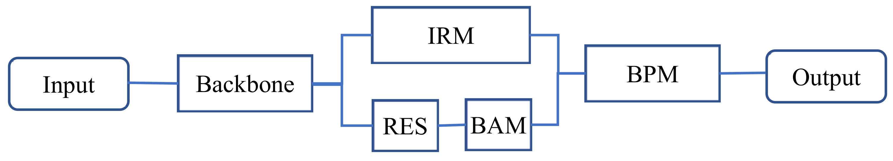
Pang et al. [12] proposed a self-interactive module (SIM) to extract features from the shallow and middle layers so that the multiscale information can be adaptively extracted from the data. The multiscale information was used to deal with the scale changes of salient objects, which effectively meets the multiscale requirements of SOD tasks. Inspired by reference [12], the interactive residual model (IRM) was designed in this paper. IRM models learned the multiscale features of a single convolution block in two different resolutions, interactively. To extract richer features and reduce redundant information, IRM removed the original feedback mechanism of SIM, optimized the internal sampling structure, and added a dropout block to prevent overfitting. For the deep semantic information, we used the BAM to extract the features in space and channels. The spatial attention module computed the affinity between any two feature parameters in the spatial position. For the channel information, balanced attention was also used to calculate the affinities between any two-channel maps. Finally, two attention modules were fused together to further enhance the feature representation. The complete flowchart is shown in Figure 2.
A multiscale balanced-aware interactive network (MBINet) is proposed for salient object detection. Our contributions are summarized as three items:
- An interactive residual model (IRM) was designed to capture the semantic information of multiscale features. The IRM can extract multiscale information adaptively from the samples and can deal with the scale changes better.
- We proposed a balanced-attention model (BAM), which not only captures the dependence between different features of a single sample, but considers the potential correlation between different samples, which improves the generalization ability of attention mechanism.
- To effectively fuse the output of IRMs and BAM cascade structure, an improved bi-directional propagation strategy was adopted, which can fully capture contextual in-formation of different scales, thereby improving detection performance.
2. Proposed Method
In this section, we first introduce the overall framework of the MBINet we have proposed. Figure 3 shows the network architecture. Next, we introduce the principle of the interactive residual model and formula derivation in detail in Section 2.2. In Section 2.3, we describe how to derive the balanced attention model step-by-step and the implementation details. Finally, we effectively merge all the features together by introducing the BPM to reflect the multiscale feature fusion further.
2.1. Network Architecture
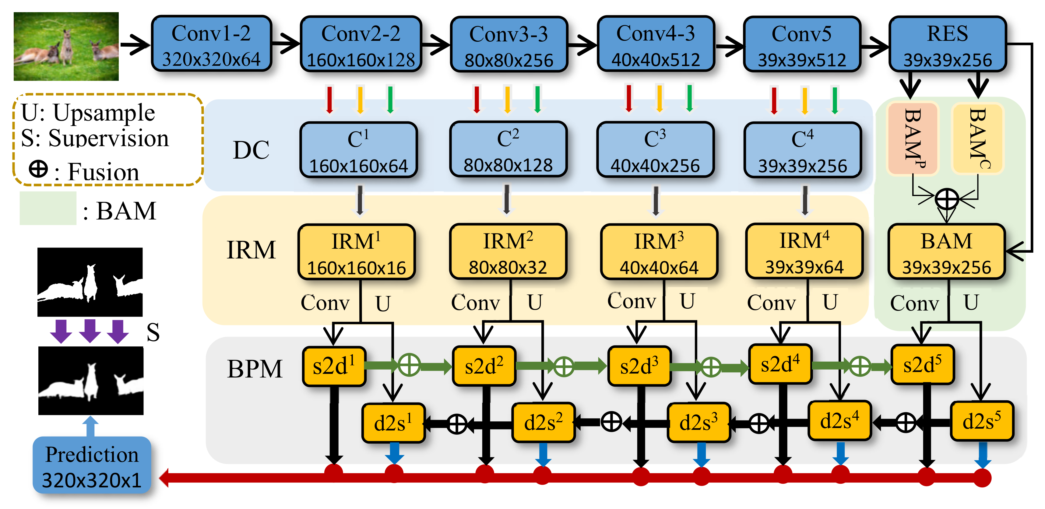
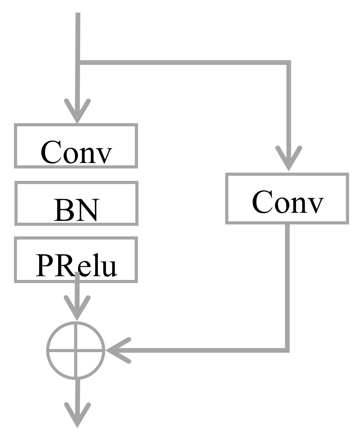
In our model, the VGG-16 [36] network is used as the pre-training backbone network. Similarly to other SOD methods, we removed all fully connected layers and the last pooling layer, and marked the side outputs of different scales as {Conv1, Conv2, Conv3, Conv4, Conv5}. Since the receptive field of Conv1 was too small and there was too much noise, we decided to only use the side output of Conv2–5 for feature extraction. First, we used the dilated convolution (DC) with the dilation rate of {1, 2, 4} to extract the features of the side output, denoted as C = {C1, C2, C3, C4}, and send the output result to the interactive residual networks (IRMs) model. The characteristic of DC is to expand the receptive field with a fixed-size convolution kernel. The larger the receptive field, the richer the semantic information captured. The purpose of introducing DC is to extract features of different scales from the same feature map. However, IRMs use fixed-size convolution kernels to extract feature maps of different scales. Through complementary learning of DC and IRMs, more effective multiscale features can be obtained. In addition, we added a residual structure (RES) after Conv5, as shown in Figure 4, in order to reduce channel numbers of in-depth features and to pass the output features to a BAM based on both spatial and channel directions. The in-depth information output by BAM was fused together, and the output of IRMs was used as input to the bidirectional propagation network [4]. A prediction graph was generated at each fusion node. Next, we will introduce these models in detail.
2.2. Interactive Residual Model
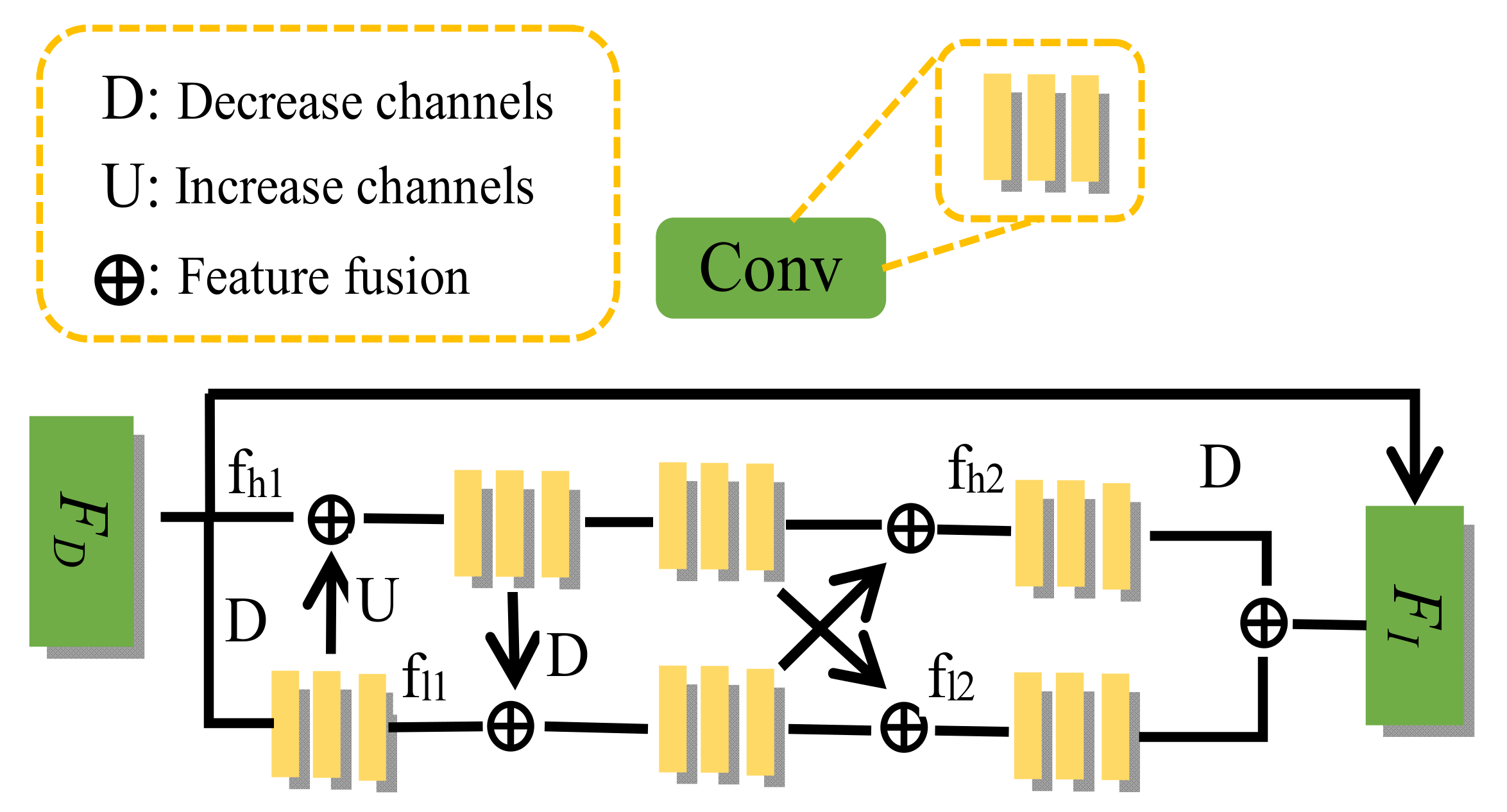
The side output of different depths contains different features of information. We use DC to extract the features from the side output of the encoder, and the output result is expressed as . The function of DC is to expand the receptive field, which can improve the representation ability of small features and ensure the integrity of feature extraction. However, while improving the integrity of the features, the noise is also preserved. In order to further refine the features and complement DC, we introduce an interactive residual model (IRM), as shown in Figure 5. IRM divides the input features into two in a pooling manner, denoted as and , where . To extract the features of two resolutions in parallel, and fuse the two output results with their respective sizes, denoted as and , the expressions are as follows:
where represents the level of the side output depth, and represent the de-convolution and pooling operations on the feature, and represents channel numbers for reducing the feature. Channel numbers of is 1/4 of the number of input channels, and the channel numbers of are the same as the number of input channels. To keep the input and output consistent and have the same size as the input, we upsampled , downchanneled , and merged the results of the two branches, denoted as . In order to facilitate optimization, each feature size change underwent normalization and nonlinear processing, and the input feature was processed again, and the was changed directly to the output port of IRMs after changing the channel. The whole process can be expressed by the following formula:
2.3. Balanced-Attention Model
The attention mechanism is widely used in computer vision, and it is also popular in salient detection. Some attention models [35,37,38,39,40] have also been proposed in recent years. Self-attention is used to compute similarity between local features in order to obtain large-scale dependence. Specifically, the input features are linearly projected into a query matrix , a key matrix , and a value matrix [33]. The self-attention model can be formulated as:
where represents the number of pixels, is the corresponding pixel value, and represent the number of feature dimensions, and represents the output. Obviously, the high computational complexity of self-attention is an obvious disadvantage. Based on this, the beyond-attention model uses two storage units and to substitute the three self-attention matrices , , and , for calculating the correlation between feature pixels and external storage unit , and using double-normalization to complete the normalization of features. Since is a learnable parameter, affected by the whole datasets, it acts as a medium for the association of all features and is the memory of the whole training datasets. Double-normalization is essentially the nesting of softmax, at the expense of computational cost. Although features can be further refined and the impact of noise can be reduced, the effect is not obvious for deep features that have been processed multiple times. To this end, combining the advantages of the two attention models above, we proposed a model named the balanced-attention model (BAM). The details of the BAM are shown in Figure 6.
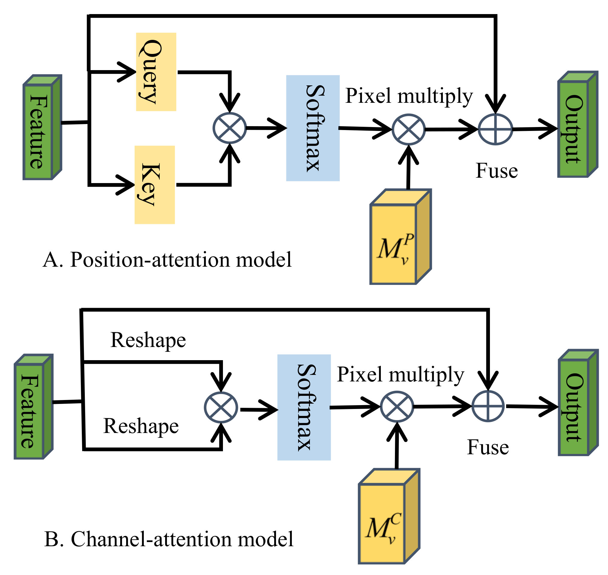
First of all, we extracted the deep features in the spatial position, and transformed the input feature projection into a query matrix and a key matrix , where is the number of pixels, then multiplied the transpose matrix of and , and calculated the resulting matrix using the soft max function. The result is the spatial correlation between different pixels. Then a linear layer was used as the memory to share the whole datasets, and the input was fused into the above operation results to get the final output . The whole process can be formulated as:
where represents the output feature in the spatial direction.
While paying attention to the affinity relationship between different location features, we also noticed that the interdependence between channel mappings would affect the feature representation of specific semantics. Therefore, we also used the attention mechanism in the channel direction to improve the interdependence between channels. First of all, the input feature was transformed into , and then the multiplication operation was performed between and its own transpose matrix, and the resulting square matrix was sent to the softmax classification function to calculate the pixel correlation degree in the channel direction. Then a linear layer was used as the memory to transform the result to , and the final result is represented by . The whole process can be expressed by the following formula:
2.4. Model Interaction and Integration
In order to strengthen the interdependence between different features, we fused the output results in the space and channel direction together and denoted it as . In addition, the BAM was regarded as an independent part, and the detected semantic information and the output characteristics of the IRMs were fused in a propagation mode. First, we changed the number of output feature channels for BAM and IRMs to 21 and produced two results of the same dimension simultaneously. Then, one of the results of each module was compiled into a group for cascade fusion in the direction from shallow to deep, and the other group was cascaded and fused in the direction from deep to shallow, and the output obtained after each level was fused as the predicted value. The above process is referred to as the bidirectional propagation model (BPM), as shown in BPM in Figure 3. Take as the IRMs output layer and as the BAM output layer. The features are gradually superimposed in two directions from shallow to deep and from deep to shallow, and the output of each side is used as the final prediction result. The whole process can be expressed by the following formula:
Among them, is the feature fusion operation, is the feature stitching operation according to the channel direction, and are the results of after the reduced channel, is the output of each level from shallow to deep, and is similar. Finally, we used the standard binary cross-entropy to train the predicted value; the expression is as follows:
where represents the true value of pixel , and represents the predicted value of pixel training. The calculation process is as follows:
3. Experiment
3.1. Experimental Setup
Datasets: We evaluated the proposed model on six benchmark datasets: DUT-OMRON [19], DUTS [41], ECSSD [42], PASCAL-S [43], HKU-IS [44], and SOD [45]. DUTS contains 10,553 training images and 5019 testing images, of which the images used for training are called DUTS-TR and the images used for testing are called DUTS-TE, and both contain complex scenes. ECSSD contains 1000 semantic images with various complex scenes. PASCAL-S contains 850 images with cluttered backgrounds and complex salient regions, which are from the verification set of the PASCAL VOC 2010 segmentation datasets. HKU-IS contains 4447 images with high-quality annotations, and has multiple unconnected salient objects in many images. DUT-OMRON contains 5168 challenging images. Most of the images in these datasets contain one or more salient objects with complex backgrounds. The SOD datasets have 300 very challenging images, most of which contain multiple objects with low contrast or connection with image boundaries.
Evaluation criteria: We used three metrics to evaluate the performance of the proposed model MBINet and other state-of-the-art SOD algorithms. The three metrics were -measure [46], mean absolute error (MAE) [15], and S-measure [47]. The -measure was computed by the weighted harmonic mean of precision value and recall value, and its expression is:
where is generally set to 0.3 for weight precision. Since the precision value and recall value are calculated on the basis of a binary image, we first needed to threshold the prediction map to a binary image. Threshold calculation is to combine multiple thresholds to calculate the appropriate value adaptively. Different thresholds corresponded to different scores. Here we reported the maximum score of all thresholds. MAE is calculated to measure the average difference between the predicted map and the ground-truth map . The expression of MAE is:
where W and H are the width and height of the image respectively. S-measure calculates the structural similarity of object perception and region perception between the predicted map and the ground-truth map, and the expression is:
where is set to 0.5 [47].
Implementation details: We implemented our proposed model based on the Pytorch framework. To facilitate comparison with other works, we chose VGG-16 [36] as the backbone network. Following most existing methods, we used the DUTS-TR datasets as a training set, the SOD datasets as a validation set to update best weights, the DUTS-TE, ECSSD, PASCAL-S, HKU-IS, and DUT-OMRON as testing sets, and the DUTS-TE datasets as the benchmark for ablation experiments. Our network was based on the NVIDIA GTX 1080 Ti GPU, and the operating system was trained on Ubuntu 16.04. To ensure that the model converges, we used the Adam [48] optimizer to train our model. The initial learning rate was set to 1e-4, the batch size was set to 8, and the resolution was adjusted to 320 × 320. The training process of our model took about 18 h and converged after 22 epochs.
3.2. Ablation Studies
The proposed model is composed of three parts: IRM, BAM, and BPM. In this section, we conducted ablation studies to verify the effectiveness of each module combination. The experimental setup follows Table 1, and we mainly report the results using the DUTS-TE datasets.
Effectiveness of the BAM: BAM combines the advantages of the self-attention and the beyond-attention models. These attention models are embedded into our model, and compared on the DUTS-TE datasets, and the results are recorded in Table 2.
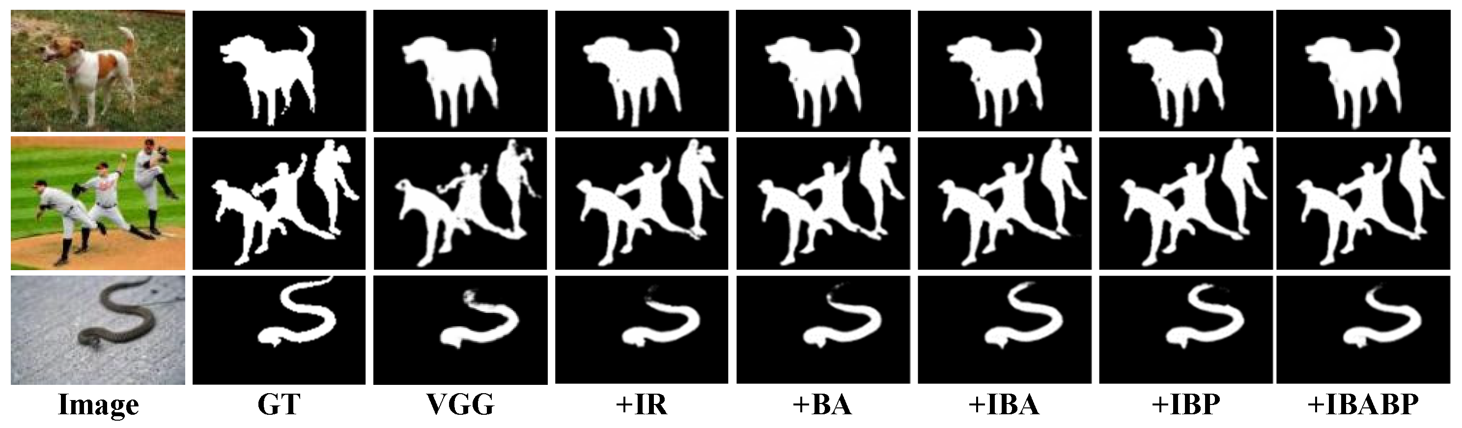
We found that the performance of BAM was better than that of the self-attention and the external attention models alone. Especially in terms of MAE, which increased by 1.72% and 3.45% compared with the beyond-attention and self-attention models respectively, and the visual effects are shown in Figure 7. We can see that BAM can capture richer contextual information.
Effectiveness of the IRM and BPM: IRM mainly processes the features of the shallow layer and the middle layer in order to further refine the features extracted by DC. BPM is a feature fusion mechanism between IRM and BAM. In Table 1, different combinations of the three models are shown. From Table 1, it is obviously that the integration of these independent modules can complement each other.
For a more comprehensive analysis of IRM, we further studied the impact of the number of dilate convolutions and the dilation rate. First of all, we tested the number of convolutions when the dilation rate is {1, 2, 4}. We conducted five different values experiments, and recorded the test results in Table 3. It can be found from Table 3 that = 3 has the best performance. Next, in order to test the influence of the dilation rate, we chose five different sets of dilation rates: {1,1,1}, {1,2,3}, {1,3,5}, {1,2,4} and {1,4,7}, and recorded the test results in Table 4. We found that the performance is the best when the dilation rate is {1,2,4}. Therefore, we finally determined the dilation rate of {1, 2, 4}.
3.3. Comparison with State-of-the-Art
In this section, we compare our proposed module with the state-of-the-art salient detection methods, including RFCN [10], MCDL [22], LEGS [23], Amulet [28], CANet [34], MDF [44], RSD [49], DSS [50], NLDF [51], DCL [52], BSCA [53], ELD [54], and UCF [55]. For fair comparison, the salient maps of the above methods are provided by the author or calculated by running the source code.
Quantitative comparison: We evaluated the proposed method from the three aspects of -measure, MAE, and S-measure, and also compared it with other SOD methods, as shown in Table 5. It can be seen from the results that our method is significantly better than other salient detection methods. In particular, in terms of MAE, the best scores are obtained on all five datasets, and the performance is improved on average compared to the second-best method.
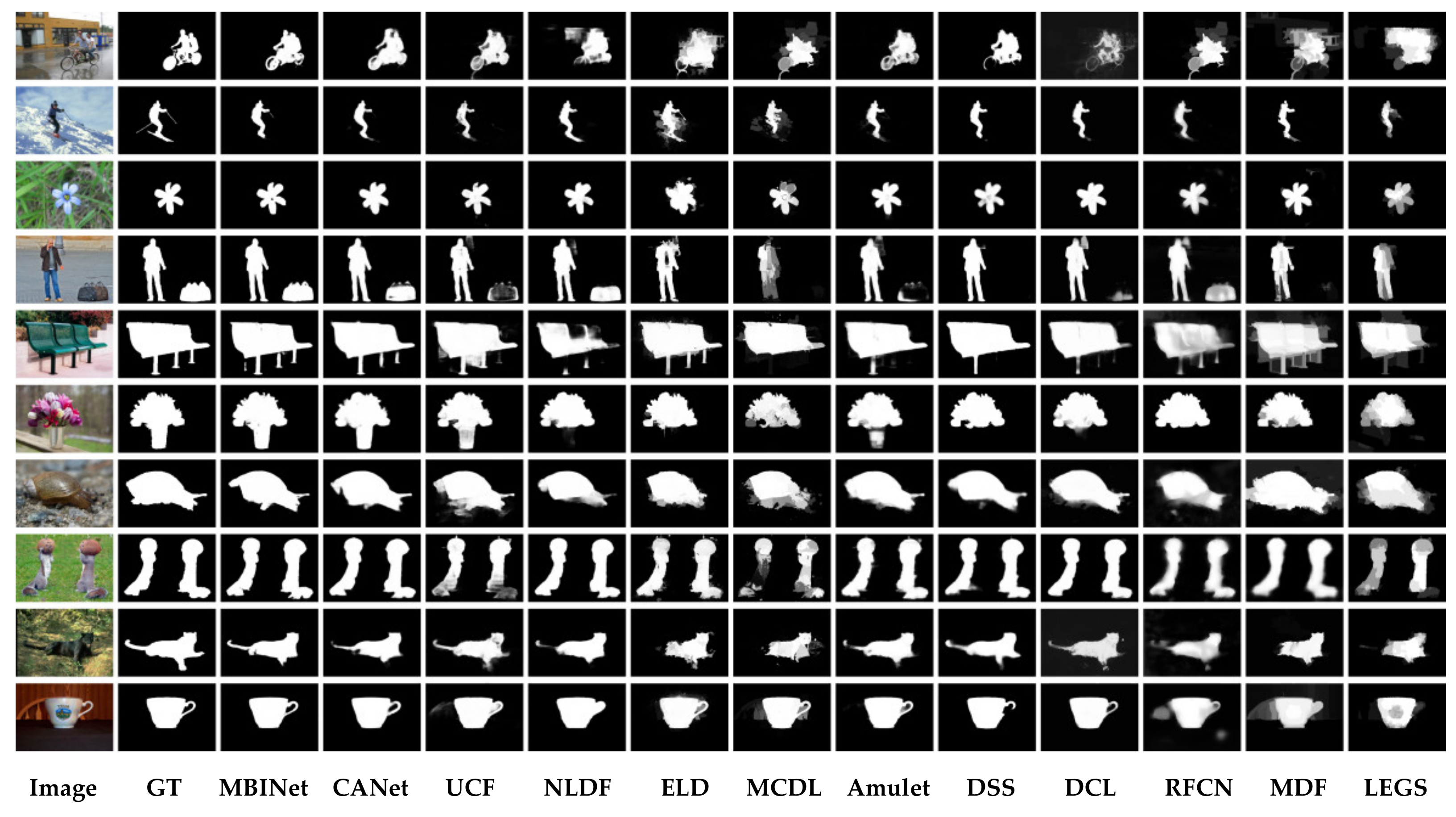
Qualitative evaluation: Figure 8 shows some representative examples. These examples reflect different scenes, including small objects, complex scenes, and images with low contrast between foreground and background. It can be seen from the figure that the proposed method can predict the foreground area more accurately and completely.
4. Conclusions
In this paper, we proposed a novel multiscale balanced-attention interactive perception network for salient object detection. First, we used dilated convolutions to extract multiscale features on the side output of the encoder. Next, interactive residual modules (IRMs) were designed to further refine the edge information of the multiscale features. Thus, the features, extracted by the interactive residual network and the dilated convolutions module, were complementary to each other, and the noise was suppressed. In addition, we proposed a balanced-attention model (BAM), which captured the deep context information of the objects in both spatial and channel directions respectively. The ablation experiments showed that the BAM’s and IRM’s cascade structures could extract richer semantic information for different scales features. Finally, in order to better describe and accurately locate the predicted object, we adopted the improved bi-directional propagation module (BPM) to improve the interdependence between different features. Whether IRM and BPM modules were cascaded for testing, or BAM and BPM modules were cascaded for testing, the results showed that the bi-directional propagation module could more effectively integrate multiscale features. In conclusion, the experimental evaluation on five datasets demonstrated that the designed method could predict the saliency map more accurately than the existing partial saliency detection methods under different evaluation metrics. In further research, we will plan to maintain the existing strengths of our method while considering the challenging problem of model lightweighting. In the future, we will try to further optimize our solution to achieve better predictive performance.
Author Contributions
H.Y. conceived the entire design method, and guided the creation of the model and participated in further improving the manuscript. R.C.’s responsibility was to build the entire network model, carry out the experiment and draft the initial manuscript. D.D. helped motivate the research. And all authors participated in further improving the manuscript. All authors have read and agreed to the published version of the manuscript.
Funding
This work was supported in part by the National Natural Science Foundation of China under Grant No. 62,167,002 and Grant No. 61862013, in part by the Guangxi Science and Technology Base and Talent Special Project under Grant No. AD18281084.
Institutional Review Board Statement
Not applicable.
Informed Consent Statement
Not applicable.
Data Availability Statement
The research uses the DUTS, SOD, PASCAL-S, ECSSD, HKU-IS and DUT-OMROM datasets from computer vision standard datasets. Datasets are available upon request.
Conflicts of Interest
All authors declare that they have no conflict of interest.
References
- Gkelios, S.; Sophokleous, A.; Plakias, S.; Boutalis, Y.; Chatzichristofis, S. Deep convolutional features for image retrieval. Expert Syst. Appl. 2021, 177, 114940. [Google Scholar] [CrossRef]
- Radenović, F.; Tolias, G.; Chum, O. Fine-Tuning CNN Image Retrieval with No Human Annotation. IEEE Trans. Pattern Anal. Mach. Intell. 2018, 41, 1655–1668. [Google Scholar] [CrossRef] [PubMed] [Green Version]
- Cheng, X.; Li, E.; Fu, Z. Residual Attention Siamese RPN for Visual Tracking. In Proceedings of the Chinese Conference on Pattern Recognition and Computer Vision (PRCV), Nanjing, China, 16–18 October 2020. [Google Scholar]
- Fu, J.; Liu, J.; Tian, H.; Li, Y.; Bao, Y.; Fang, Z.; Lu, H. Dual Attention Network for Scene Segmentation. In Proceedings of the 2019 IEEE/CVF Conference on Computer Vision and Pattern Recognition (CVPR), Long Beach, CA, USA, 15–20 June 2019; IEEE: Piscataway, NJ, USA, 2019. [Google Scholar]
- Liu, Y.; Han, J.; Zhang, Q.; Shan, C. Deep Salient Object Detection with Contextual Information Guidance. IEEE Trans. Image Process. 2019, 29, 360–374. [Google Scholar] [CrossRef] [PubMed] [Green Version]
- Gu, K.; Zhai, G.; Yang, X.; Zhang, W.; Chen, C.W. Automatic contrast enhancement technology with saliency preservation. IEEE Trans. Circ. Syst. Video Technol. 2015, 25, 1480–1494. [Google Scholar] [CrossRef]
- Wu, J.; Chang, L.; Yu, G. Effective Data Decision-Making and Transmission System Based on Mobile Health for Chronic Disease Management in the Elderly. IEEE Syst. J. 2021, 15, 5537–5548. [Google Scholar] [CrossRef]
- Chang, L.; Wu, J.; Moustafa, N.; Bashir, A.; Yu, K. AI-Driven Synthetic Biology for Non-Small Cell Lung Cancer Drug Effectiveness-Cost Analysis in Intelligent Assisted Medical Systems. IEEE J. Biomed. Health Inform. 2021, 34874878. [Google Scholar] [CrossRef] [PubMed]
- Yu, G.; Wu, J. Efficacy prediction based on attribute and multi-source data collaborative for auxiliary medical system in developing countries. Neural Comput. Appl. 2022, 1–16. [Google Scholar] [CrossRef]
- Wang, L.; Wang, L.; Lu, H.; Zhang, P.; Ruan, X. Salient Object Detection with Recurrent Fully Convolutional Networks. IEEE Trans. Pattern Anal. Mach. Intell. 2018, 41, 1734–1746. [Google Scholar] [CrossRef] [PubMed]
- Chen, S.; Tan, X.; Wang, B.; Hu, X. Reverse Attention for Salient Object Detection. Computer Vision—ECCV 2018. In Lecture Notes in Computer Science; Springer: Cham, Switzerland, 2018; Volume 11213. [Google Scholar]
- Pang, Y.; Zhao, X.; Zhang, L.; Lu, H. Multi-Scale Interactive Network for Salient Object Detection. In Proceedings of the 2020 IEEE/CVF Conference on Computer Vision and Pattern Recognition, Seattle, WA, USA, 13–19 June 2020. [Google Scholar]
- Itti, L.; Koch, C.; Niebur, E. A model of saliency-based visual attention for rapid scene analysis. IEEE Trans. Pattern Anal. Mach. Intell. 1998, 20, 1254–1259. [Google Scholar] [CrossRef] [Green Version]
- Borji, A.; Itti, L. Exploiting local and global patch rarities for saliency detection. In Proceedings of the 2012 IEEE Conference on Computer Vision and Pattern Recognition (CVPR), Providence, RI, USA, 16–21 June 2012; IEEE: Piscataway, NJ, USA, 2012. [Google Scholar]
- Perazzi, F.; Krahenbuhl, P.; Pritch, Y.; Hornung, A. Saliency filters: Contrast based filtering for salient region detection. In Proceedings of the 2012 IEEE Conference on Computer Vision and Pattern Recognition, Providence, RI, USA, 16–21 June 2012. [Google Scholar]
- Cheng, M.M.; Mitra, N.J.; Huang, X.; Torr, P.H.; Hu, S.M. Global contrast based salient region detection. IEEE Trans. Pattern Anal. Mach. Intell. 2014, 37, 569–582. [Google Scholar] [CrossRef] [PubMed] [Green Version]
- Jiang, Z.; Davis, L.S. Sub modular Salient Region Detection. In Proceedings of the 2013 IEEE Conference on Computer Vision and Pattern Recognition (CVPR), Portland, OR, USA, 23–28 June 2013. [Google Scholar]
- Li, X.; Lu, H.; Zhang, L.; Ruan, X.; Yang, M. Saliency Detection via Dense and Sparse Reconstruction. In Proceedings of the IEEE International Conference on Computer Vision, Sydney, NSW, Australia, 1–8 December 2013. [Google Scholar]
- Yang, C.; Zhang, L.; Lu, H.; Ruan, X.; Yang, M. Saliency detection via graph-based manifold ranking. In Proceedings of the IEEE Conference on Computer Vision and Pattern Recognition, Portland, OR, USA, 23–28 June 2013. [Google Scholar]
- Borji, A.; Cheng, M.M.; Jiang, H.; Li, J. Salient object detection: A benchmark. IEEE Trans. Image Process. 2015, 24, 5706–5722. [Google Scholar] [CrossRef] [PubMed] [Green Version]
- Sun, L.; Chen, Z.; Wu, Q.M.J.; Zhao, H.; He, W.; Yan, X. AMPNet: Average-and Max-Pool Networks for Salient Object Detection. IEEE Trans. Circuits Syst. Video Technol. 2021, 31, 4321–4333. [Google Scholar] [CrossRef]
- Rui, Z.; Ouyang, W.; Li, H.; Wang, X. Saliency detection by multi-context deep learning. In Proceedings of the 2015 IEEE Conference on Computer Vision and Pattern Recognition (CVPR), Boston, MA, USA, 7–12 June 2015. [Google Scholar]
- Wang, L.; Lu, H.; Xiang, R.; Ming, Y. Deep networks for saliency detection via local estimation and global search. In Proceedings of the 2015 IEEE Conference on Computer Vision and Pattern Recognition (CVPR), Boston, MA, USA, 7–12 June 2015. [Google Scholar]
- Zhang, X.; Wang, T.; Qi, J.; Lu, H.; Wang, H. Progressive Attention Guided Recurrent Network for Salient Object Detection. In Proceedings of the 2018 IEEE/CVF Conference on Computer Vision and Pattern Recognition, Salt Lake City, UT, USA, 18–23 June 2018. [Google Scholar]
- Qin, X.; Zhang, Z.; Huang, C.; Gao, C.; Dehghan, M.; Jagersand, M. BASNet: Boundary-Aware Salient Object Detection. In Proceedings of the 2019 IEEE/CVF Conference on Computer Vision and Pattern Recognition (CVPR), Long Beach, CA, USA, 15–20 June 2019. [Google Scholar]
- Wu, R.; Feng, M.; Guan, W.; Wang, D.; Lu, H.; Ding, E. A Mutual Learning Method for Salient Object Detection with Intertwined Multi-Supervision. In Proceedings of the 2019 IEEE/CVF Conference on Computer Vision and Pattern Recognition (CVPR), Long Beach, CA, USA, 15–20 June 2019. [Google Scholar]
- Wang, W.; Zhao, S.; Shen, J.; Hoi, S.; Borji, A. Salient Object Detection with Pyramid Attention and Salient Edges. In Proceedings of the 2019 IEEE/CVF Conference on Computer Vision and Pattern Recognition (CVPR), Long Beach, CA, USA, 15–20 June 2019. [Google Scholar]
- Zhang, P.; Wang, D.; Lu, H.; Wang, H.; Ruan, X. Amulet: Aggregating Multi-level Convolutional Features for Salient Object Detection. IEEE Comput. Soc. 2017, 202–211. [Google Scholar] [CrossRef] [Green Version]
- Lu, Z.; Ju, D.; Lu, H.; You, H.; Gang, W. A Bi-Directional Message Passing Model for Salient Object Detection. In Proceedings of the 2018 IEEE/CVF Conference on Computer Vision and Pattern Recognition (CVPR), Salt Lake City, UT, USA, 18–23 June 2018. [Google Scholar]
- He, J.; Zhang, S.; Yang, M.; Shan, Y.; Huang, T. BDCN: Bi-Directional Cascade Network for Perceptual Edge Detection. IEEE Trans. Pattern Anal. Mach. Intell. 2020, 44, 100–113. [Google Scholar] [CrossRef] [PubMed]
- Zhao, T.; Xiangqian, W. Pyramid feature attention network for saliency detection. In Proceedings of the 2019 IEEE/CVF Conference on Computer Vision and Pattern Recognition, Long Beach, CA, USA, 15–20 June 2019. [Google Scholar]
- Geng, Z.; Guo, M.H.; Chen, H.; Li, X.; Wei, K.; Lin, Z. Is attention better than matrix decomposition? In Proceedings of the 2015 International Conference on Learning Representation, A Virtual Event. 28 December 2021. [Google Scholar]
- Vaswani, A.; Shazeer, N.; Parmar, N.; Uszkoreit, J.; Jones, L.; Gomez, A.; Kaiser, L.; Polosukhin, I. Attention is all you need. In Proceedings of the Advances in Neural Information Processing Systems (NIPS), Long Beach, CA, USA, 4 December 2017. [Google Scholar]
- Li, J.; Pan, Z.; Liu, Q.; Cui, Y.; Sun, Y. Complementarity-Aware Attention Network for Salient Object Detection. IEEE Trans. Cybern. 2020, 1–14. [Google Scholar] [CrossRef] [PubMed]
- Guo, M.H.; Liu, Z.N.; Mu, T.J.; Hu, S.M. Beyond Self-attention: External Attention using Two Linear Layers for Visual Tasks. In Proceedings of the 2021 IEEE Conference on Computer Vision and Pattern Recognition (CVPR), A Virtual Event. 19 June 2021. [Google Scholar]
- Simonyan, K.; Zisserman, A. Very Deep Convolutional Networks for Large-Scale Image Recognition. In Proceedings of the 2015 International Conference on Learning Representation, San Diego, CA, USA, 9 May 2015. [Google Scholar]
- Guo, M.H.; Cai, J.X.; Liu, Z.N.; Mu, T.; Martin, R.; Hu, S. PCT: Point Cloud Transformer. Comput. Vis. Media 2020, 7, 187–199. [Google Scholar] [CrossRef]
- Hu, X.; Fu, C.-W.; Zhu, L.; Wang, T.; Heng, P.-A. SAC-Net: Spatial Attenuation Context for Salient Object Detection. IEEE Trans. Circuits Syst. Video Technol. 2021, 31, 1079–1090. [Google Scholar] [CrossRef]
- Liu, N.; Han, J. DHSNet: Deep Hierarchical Saliency Network for Salient Object Detection. In Proceedings of the 2016 IEEE/CVF Conference on Computer Vision & Pattern Recognition, Las Vegas, NV, USA, 27–30 June 2016. [Google Scholar]
- Huang, Z.; Wang, X.; Wei, Y.; Huang, L.; Shi, H.; Liu, W.; Huang, T. CCNet: Criss-Cross Attention for Semantic Segmentation. In Proceedings of the IEEE/CVF International Conference on Computer Vision, Seoul, Korea, 27 October 2019; pp. 603–612. [Google Scholar]
- Wang, L.; Lu, H.; Wang, Y.; Feng, M.; Wang, D.; Yin, B.; Ruan, X. Learning to Detect Salient Objects with Image-Level Supervision. In Proceedings of the IEEE Conference on Computer Vision & Pattern Recognition, Honolulu, HI, USA, 21–26 July 2017. [Google Scholar]
- Yan, Q.; Li, X.; Shi, J.; Jia, J. Hierarchical Saliency Detection. In Proceedings of the 2013 IEEE Conference on Computer Vision and Pattern Recognition (CVPR), Portland, OR, USA, 23–28 June 2013; IEEE: Piscataway, NJ, USA, 2013. [Google Scholar]
- Li, Y.; Hou, X.; Koch, C.; Rehg, J.; Yuille, A. The secrets of salient object segmentation. In Proceedings of the IEEE Conference on Computer Vision and Pattern Recognition, Columbus, OH, USA, 23–28 June 2014. [Google Scholar]
- Li, G.; Yu, Y. Visual Saliency Based on Multiscale Deep Features. In Proceedings of the 2015 IEEE Conference on Computer Vision and Pattern Recognition (CVPR), Boston, MA, USA, 7–12 June 2015. [Google Scholar]
- Movahedi, V.; Elder, J.H. Design and perceptual validation of performance measures for salient object segmentation. In Proceedings of the Computer Vision & Pattern Recognition Workshops, San Francisco, CA, USA, 13–18 June 2010. [Google Scholar]
- Achanta, R.; Hemami, S.; Estrada, F.; Susstrunk, S. Frequency-tuned salient region detection. In Proceedings of the 2009 IEEE Conference on Computer Vision and Pattern Recognition (CVPR), Miami, FL, USA, 20–25 June 2009. [Google Scholar]
- Fan, D.P.; Cheng, M.M.; Liu, Y.; Li, T.; Borji, A. Structure-measure: A New Way to Evaluate Foreground Maps. In Proceedings of the IEEE International Conference on Computer Vision, Venice, Italy, 22–29 October 2017; pp. 4548–4557. [Google Scholar]
- Kingma, D.; Ba, J. Adam: A Method for Stochastic Optimization. In Proceedings of the 2015 International Conference on Learning Representation, San Diego, CA, USA, 9 May 2015. [Google Scholar]
- Islam, M.A.; Kalash, M.; Bruce, N.D.B. Revisiting salient object detection: Simultaneous detection, ranking, and subitizing of multiple salient objects. In Proceedings of the 2018 IEEE/CVF Conference on Computer Vision and Pattern Recognition, Salt Lake City, UT, USA, 18–23 June 2018. [Google Scholar]
- Hou, Q.; Cheng, M.M.; Hu, X.; Borji., A.; Tu., Z.; Torr., P.H. Deeply Supervised Salient Object Detection with Short Connections. In Proceedings of the 2017 IEEE Conference on Computer Vision and Pattern Recognition (CVPR), Honolulu, HI, USA, 21–26 July 2017. [Google Scholar]
- Luo, Z.; Mishra, A.; Achkar, A.; Eichel, J.; Li, S.; Jodoin, P. Non-local Deep Features for Salient Object Detection. In Proceedings of the 2017 IEEE Conference on Computer Vision and Pattern Recognition (CVPR), Honolulu, HI, USA, 21–26 July 2017. [Google Scholar]
- Li, G.; Yu, Y. Deep Contrast Learning for Salient Object Detection. In Proceedings of the 2016 IEEE Conference on Computer Vision and Pattern Recognition (CVPR), Las Vegas, NV, USA, 27–30 June 2016. [Google Scholar]
- Yao, Q.; Lu, H.; Xu, Y.; Wang, H. Saliency detection via Cellular Automata. In Proceedings of the 2015 IEEE Conference on Computer Vision and Pattern Recognition (CVPR), Boston, MA, USA, 7–12 June 2015. [Google Scholar]
- Lee, G.; Tai, Y.W.; Kim, J. Deep Saliency with Encoded Low Level Distance Map and High Level Features. In Proceedings of the 2016 IEEE Conference on Computer Vision and Pattern Recognition (CVPR), Las Vegas, NV, USA, 27–30 June 2016. [Google Scholar]
- Zhang, P.; Dong, W.; Lu, H.; Wang, H.; Yin, B. Learning Uncertain Convolutional Features for Accurate Saliency Detection. In Proceedings of the 2017 IEEE International Conference on Computer Vision (ICCV), Venice, Italy, 22–29 October 2017. [Google Scholar]
Figure 1.
Example of background filtering based on salient object detection.

Figure 2.
Complete flowchart of MBINet.

Figure 3.
The overall framework of the model. IRM: interactive residual model. BAM: balanced-attention model. BPM: bidirectional propagation model. DC: hollow convolution. RES: residual structure. U: upsampling. S: supervision. s2d: from shallow to deep. d2s: from deep to shallow.
Figure 3.
The overall framework of the model. IRM: interactive residual model. BAM: balanced-attention model. BPM: bidirectional propagation model. DC: hollow convolution. RES: residual structure. U: upsampling. S: supervision. s2d: from shallow to deep. d2s: from deep to shallow.

Figure 4.
Structure of RES. Conv: convolution operation. BN: regularization. PRelu: activation function.
Figure 4.
Structure of RES. Conv: convolution operation. BN: regularization. PRelu: activation function.

Figure 5.
The structure of the interactive residual model.

Figure 6.
Balance the structure of the attention model. The details of the position-attention model and channel-attention model are illustrated in (A) and (B).
Figure 6.
Balance the structure of the attention model. The details of the position-attention model and channel-attention model are illustrated in (A) and (B).

Figure 7.
Visual comparison of each module. GT: ground truth; IR: IRM; BA: BAM; IBA: IRM + BAM; BP: IRM + BPM; IBABP: IRM + BAM + BPM.
Figure 7.
Visual comparison of each module. GT: ground truth; IR: IRM; BA: BAM; IBA: IRM + BAM; BP: IRM + BPM; IBABP: IRM + BAM + BPM.

Figure 8.
Visual comparisons of different methods.


Table 1.
Ablation analysis on the DUTS-TE datasets. BAMp is the BAM submodule at the position, BAMc is the BAM submodule at the channel, and BAM means BAMp+BAMc.
Table 1.
Ablation analysis on the DUTS-TE datasets. BAMp is the BAM submodule at the position, BAMc is the BAM submodule at the channel, and BAM means BAMp+BAMc.
| No. | Model | F-Measure↑ | MAE↓ | S-Measure↑ |
|---|---|---|---|---|
| a | VGG | 0.760 | 0.074 | 0.790 |
| b | VGG + IRM | 0.782 | 0.065 | 0.803 |
| c | VGG + BAMp | 0.775 | 0.066 | 0.804 |
| d | VGG + BAMc | 0.763 | 0.069 | 0.801 |
| e | VGG + BAMp + BAMc | 0.781 | 0.066 | 0.806 |
| f | VGG + BPM | 0.777 | 0.068 | 0.801 |
| g | VGG + IRM + BAM | 0.800 | 0.061 | 0.820 |
| h | VGG + IRM + BPM | 0.789 | 0.063 | 0.809 |
| i | VGG + BAM + BPM | 0.785 | 0.060 | 0.822 |
| j | VGG + IRM + BAM + BPM | 0.809 | 0.058 | 0.824 |
Table 2.
The different models embedded and measured on the DUTS-TE datasets.
| No. | Model | F-Measure↑ | MAE↓ | S-Measure↑ |
|---|---|---|---|---|
| a | +Self-attention | 0.804 | 0.060 | 0.824 |
| b | +Beyond-attention | 0.801 | 0.059 | 0.818 |
| c | +BAM | 0.809 | 0.058 | 0.824 |
Table 3.
Evaluate convolutions on DUTS-TE. k represents the number of dilate convolutions.
| F-Measure↑ | MAE↓ | S-Measure↑ | |
|---|---|---|---|
| 1 | 0.7534 | 0.0742 | 0.7860 |
| 2 | 0.7517 | 0.0756 | 0.7859 |
| 3 | 0.7634 | 0.0711 | 0.7927 |
| 4 | 0.7578 | 0.0741 | 0.7899 |
| 5 | 0.7588 | 0.0715 | 0.7881 |
Table 4.
Evaluation of different dilation rates with the DUTS-TE datasets.
| No. | F-Measure↑ | MAE↓ | S-Measure↑ |
|---|---|---|---|
| {1,1,1} | 0.7634 | 0.0711 | 0.7927 |
| {1,2,3} | 0.7658 | 0.0710 | 0.7988 |
| {1,3,5} | 0.7683 | 0.0694 | 0.7971 |
| {1,2,4} | 0.7768 | 0.0678 | 0.8014 |
| {1,4,7} | 0.7513 | 0.0760 | 0.7848 |
Table 5.
Quantitative evaluation. Comparison of different salient detection methods (the best three results are marked as red, green, and blue respectively).
Table 5.
Quantitative evaluation. Comparison of different salient detection methods (the best three results are marked as red, green, and blue respectively).
| Model | DUTS-TE | ECSSD | PASCAL-S | HKU-IS | DUT-OMROM | ||||||||||
|---|---|---|---|---|---|---|---|---|---|---|---|---|---|---|---|
| F↑ | M↓ | S↑ | F↑ | M↓ | S↑ | F↑ | M↓ | S↑ | F↑ | M↓ | S↑ | F↑ | M↓ | S↑ | |
| Ours | 0.809 | 0.058 | 0.824 | 0.909 | 0.058 | 0.886 | 0.821 | 0.092 | 0.806 | 0.901 | 0.042 | 0.880 | 0.763 | 0.069 | 0.781 |
| CANet [34] | 0.796 | 0.056 | 0.840 | 0.907 | 0.049 | 0.898 | 0.832 | 0.120 | 0.790 | 0.897 | 0.040 | 0.895 | 0.719 | 0.071 | 0.795 |
| NLDF [51] | 0.813 | 0.065 | 0.816 | 0.905 | 0.063 | 0.875 | 0.822 | 0.098 | 0.805 | 0.902 | 0.048 | 0.878 | 0.753 | 0.080 | 0.771 |
| Amulet [28] | 0.773 | 0.075 | 0.796 | 0.911 | 0.062 | 0.849 | 0.862 | 0.092 | 0.820 | 0.889 | 0.052 | 0.886 | 0.737 | 0.083 | 0.771 |
| DCL [52] | 0.782 | 0.088 | 0.795 | 0.891 | 0.088 | 0.863 | 0.804 | 0.124 | 0.791 | 0.885 | 0.072 | 0.861 | 0.739 | 0.097 | 0.764 |
| UCF [55] | 0.771 | 0.116 | 0.777 | 0.908 | 0.080 | 0.884 | 0.820 | 0.127 | 0.806 | 0.888 | 0.073 | 0.874 | 0.735 | 0.131 | 0.748 |
| DSS [50] | 0.813 | 0.065 | 0.812 | 0.906 | 0.064 | 0.882 | 0.821 | 0.101 | 0.796 | 0.900 | 0.050 | 0.878 | 0.760 | 0.074 | 0.765 |
| ELD [54] | 0.747 | 0.092 | 0.749 | 0.865 | 0.082 | 0.839 | 0.772 | 0.122 | 0.757 | 0.843 | 0.072 | 0.823 | 0.738 | 0.093 | 0.743 |
| RFCN [10] | 0.784 | 0.091 | 0.791 | 0.898 | 0.097 | 0.860 | 0.827 | 0.118 | 0.793 | 0.895 | 0.079 | 0.859 | 0.747 | 0.095 | 0.774 |
| BSCA [53] | 0.597 | 0.197 | 0.630 | 0.758 | 0.183 | 0.725 | 0.666 | 0.224 | 0.633 | 0.723 | 0.174 | 0.700 | 0.616 | 0.191 | 0.652 |
| MDF [44] | 0.729 | 0.093 | 0.732 | 0.832 | 0.105 | 0.776 | 0.763 | 0.143 | 0.694 | 0.860 | .0129 | 0.810 | 0.694 | 0.092 | 0.720 |
| RSD [49] | 0.757 | 0.161 | 0.724 | 0.845 | 0.173 | 0.788 | 0.864 | 0.155 | 0.805 | 0.843 | 0.156 | 0.787 | 0.633 | 0.178 | 0.644 |
| LEGS [23] | 0.655 | 0.138 | - | 0.827 | 0.118 | 0.787 | 0.756 | 0.157 | 0.682 | 0.770 | 0.118 | - | 0.669 | 0.133 | - |
| MCDL [22] | 0.461 | 0.276 | 0.545 | 0.837 | 0.101 | 0.803 | 0.741 | 0.143 | 0.721 | 0.808 | 0.092 | 0.786 | 0.701 | 0.089 | 0.752 |
Publisher’s Note: MDPI stays neutral with regard to jurisdictional claims in published maps and institutional affiliations. |
© 2022 by the authors. Licensee MDPI, Basel, Switzerland. This article is an open access article distributed under the terms and conditions of the Creative Commons Attribution (CC BY) license (https://creativecommons.org/licenses/by/4.0/).
Share and Cite
MDPI and ACS Style
Yang, H.; Chen, R.; Deng, D. Multiscale Balanced-Attention Interactive Network for Salient Object Detection. Mathematics 2022, 10, 512. https://0-doi-org.brum.beds.ac.uk/10.3390/math10030512
AMA Style
Yang H, Chen R, Deng D. Multiscale Balanced-Attention Interactive Network for Salient Object Detection. Mathematics. 2022; 10(3):512. https://0-doi-org.brum.beds.ac.uk/10.3390/math10030512
Chicago/Turabian StyleYang, Haiyan, Rui Chen, and Dexiang Deng. 2022. "Multiscale Balanced-Attention Interactive Network for Salient Object Detection" Mathematics 10, no. 3: 512. https://0-doi-org.brum.beds.ac.uk/10.3390/math10030512
Note that from the first issue of 2016, this journal uses article numbers instead of page numbers. See further details here.