Subclasses of Multivalent Meromorphic Functions with a Pole of Order p at the Origin

Abstract

In this paper, we carry out a systematic study to discover the properties of a subclass of meromorphic starlike functions defined using the Mittag–Leffler three-parameter function. Differential operators involving special functions have been very useful in extracting information about the various properties of functions belonging to geometrically defined function classes. Here, we choose the Prabhakar function (or a three parameter Mittag–Leffler function) for our study, since it has several applications in science and engineering problems. To provide our study with more versatility, we define our class by employing a certain pseudo-starlike type analytic characterization quasi-subordinate to a more general function. We provide the conditions to obtain sufficient conditions for meromorphic starlikeness involving quasi-subordination. Our other main results include the solution to the Fekete–Szegő problem and inclusion relationships for functions belonging to the defined function classes. Several consequences of our main results are pointed out.

1. Introduction

$\mathbb{C},{\mathbb{Z}}^{-}$ and $\mathbb{N}$ will represent the sets of complex numbers, negative integers and natural numbers, respectively. We let ${\mathsf{\Omega }}^{*}=\{z:z\in \mathbb{C}\mathrm{and}0<\mid z\mid <1\}=\mathsf{\Omega }\setminus \left\{0\right\}$ to denote a punctured open unit disk. Furthermore, we let ${\mathcal{M}}_p$ denote the class of all analytic functions, except for a pole of order p at the origin and p-valent in the unit disc of the form

$$f\left(z\right)=z^{-p}+\sum _{k=0}^{\infty }{a}_k{z}^{k+1-p}(p\in \mathbb{N}=1,2,3,\dots ;z\in {\mathsf{\Omega }}^{*}).$$

(1)

Two well-known subclasses of ${\mathcal{M}}_p$ are the so-called meromorphic starlike functions of order $\gamma$ and meromorphic convex functions of order $\gamma$, which have the analytic characterization of the form

$$Re\left(\frac{z{f}^{{}^{\prime }}\left(z\right)}{f\left(z\right)}\right)<-\gamma \mathrm{and}Re\left(1+\frac{z{f}^{″}\left(z\right)}{f^{{}^{\prime }}\left(z\right)}\right)<-\gamma ,(z\in {\mathsf{\Omega }}^{*};0\le \gamma <p),$$

respectively. We let ${\mathcal{MS}}_p^{*}\left(\gamma \right)$ and ${\mathcal{MC}}_p\left(\gamma \right)$ denote the class of meromorphic starlike functions of order $\gamma$ and meromorphic convex functions of order $\gamma$, respectively. Furthermore, we let ${\mathcal{P}}_p$ denote the class of functions $h\left(z\right)$ analytic in $\mathsf{\Omega }$ with $h\left(0\right)=p$ and $Re\left[h\left(z\right)\right]>0$. ${\mathcal{P}}_1=\mathcal{P}$ will denote the well-known class functions with a positive real part, which has the usual normalization $h\left(0\right)=1$. For the development and study of various subclasses of meromorphic functions, refer to [1,2].

Hadamard product and subordination are the two primary tools that are employed to study various geometrically defined subclasses of analytic and meromorphic functions. Here, we let * and ≺ denote the Hadamard product and subordination, respectively. For two functions $f\left(z\right)$ given by (1) and $g\left(z\right)=z^{-p}+{\sum }_{k=0}^{\infty }{b}_k{z}^{k+1-p}$, the Hadamard product (or convolution) of f and g is defined by

$$(f*g)\left(z\right)=z^{-p}+\sum _{k=0}^{\infty }{a}_k{b}_k{z}^{k+1-p}=:(g*f)\left(z\right).$$

(2)

The Hadamard product acts as a bridge for studying geometric function theory in duality with the theory of special functions. Pertaining to the class of meromorphic functions, the study by Liu and Srivastava [3] is the most prominent study of this duality theory. Using the Hadamard product, they defined a differential operator (popularly known as the Liu–Srivastava operator) involving a generalized hypergeometric function. Here, we avoid stating the Liu–Srivastava operator, as it requires much supplementary information to be disseminated.

Several families of integral operators and differential operators were introduced using the Hadamard product (or convolution). Motivated by the work of Aouf [4] (also see [5,6,7]), in this paper we will introduce a family of differential and integral operators involving the Mittag–Leffler three-parameter function.

First, we will begin with a brief introduction of the Mittag–Leffler function. The Mittag–Leffler function arises naturally in the solutions of fractional integro-differential equations. For a detailed study on the Mittag–Leffler function and its applications, refer to [8,9,10,11]. Prabhakar [12] Equation 1.3) studied a singular integral equation with a generalized Mittag–Leffler three-parameter function in the kernel, which is defined by

$$E_{\theta ,\vartheta }^{\rho }\left(z\right)=\sum _{k=0}^{\infty }\frac{{\left(\rho \right)}_k{z}^k}{\Gamma \left(\theta k+\vartheta \right)k!},z,\theta ,\vartheta ,\rho \in \mathbb{C},Re\left(\theta \right)>0,$$

(3)

where ${\left(x\right)}_k$ will be used to denote the usual Pochhammer symbol defined by

$${\left(x\right)}_k=\frac{\Gamma (x+k)}{\Gamma \left(x\right)}=\left\{\begin{array}{cc}1\hfill & \mathrm{if}k=0\hfill \\ x(x+1)(x+2)\dots (x+k-1)\hfill & \mathrm{if}k\in \mathbb{N}.\hfill \end{array}\right.$$

The function $E_{\theta ,\vartheta }^{\rho }\left(z\right)$ is an entire function of order ${\left(Re\theta \right)}^{-1}$. For particular values of the parameter, $E_{\theta ,\vartheta }^{\rho }\left(z\right)$ coincides with well-known elementary functions, and some special functions. For example,

$$E_{1,2}^1\left(z\right)=\frac{e^z-1}{z}{E}_{3,1}^1\left(z\right)=\frac{1}{2}\left[e^{z^{1/3}}+2e^{-\frac{1}{2}{z}^{1/3}}cos\left(\frac{\sqrt{3}}{2}{z}^{1/3}\right)\right]$$

$$E_{\frac{1}{2},1}^1\left(z\right)=e^{z^2}erfc(-z),E_{\frac{1}{2},1}^1(\pm z^{1/2})=e^z\left[1+erf(\pm z^{1/2})\right]$$

where error function $erf\left(z\right)$ and the complementary error function $erfc\left(z\right)$ are defined by the formula

$$erfc\left(z\right)=1-erf\left(z\right)=1-\frac{2}{\sqrt{\pi }}{\int }_0^z{e}^{-t^2}dt.$$

The following relationship between the Prabhakar function and generalized hypergeometric function is known to hold:

$$E_{m,\vartheta }^{\rho }\left(z\right)=\frac{1}{\Gamma \left(\vartheta \right)}{}_1{F}_m\left(\rho ;\frac{\vartheta }{m},\frac{\vartheta +1}{m},\dots ,\frac{\vartheta +m-1}{m};\frac{z}{m^m}\right),m\in \mathbb{N},$$

where ${}_r{F}_s$ (the generalized hypergeometric function) is defined by the formula

$${}_r{F}_s({\alpha }_1,{\alpha }_2,\dots ,{\alpha }_r;{\beta }_1,{\beta }_2,\dots ,{\beta }_s;z)=\sum _{k=0}^{\infty }\frac{{\left({\alpha }_1\right)}_k\dots {\left({\alpha }_r\right)}_k}{{\left({\beta }_1\right)}_k\dots {\left({\beta }_s\right)}_k}\frac{z^k}{k!}.$$

$$({\alpha }_1,\dots ,{\alpha }_r\in \mathbb{C}\mathrm{and}{\beta }_j\in \mathbb{C}\setminus {\mathbb{Z}}_0^{-};{\mathbb{Z}}_0^{-}=0,-1,-2,\dots ;j=1,\dots ,s).$$

Corresponding to $E_{\theta ,\vartheta }^{\rho }\left(z\right)$, we define the function

$${\mathcal{K}}_{\theta ,\vartheta }^{\rho }\left(z\right)=z^{-p}\Gamma \left(\vartheta \right)E_{\theta ,\vartheta }^{\rho }\left(z\right)=z^{-p}+\sum _{k=0}^{\infty }\frac{\Gamma \left(\vartheta \right){\left(\rho \right)}_{k+1}}{\Gamma \left[\vartheta +\theta (k+1)\right](k+1)!}{z}^{k+1-p}.$$

(4)

We now define the following operator ${\mathcal{R}}_{\lambda }^{m,p}(\theta ,\vartheta ,\rho )f:{\mathsf{\Omega }}^{*}⟶{\mathsf{\Omega }}^{*}$ by

$${\mathcal{R}}_{\lambda }^{0,p}(\theta ,\vartheta ,\rho )f\left(z\right)=(f*{\mathcal{K}}_{\theta ,\vartheta }^{\rho })\left(z\right)$$

$${\mathcal{R}}_{\lambda }^{1,p}(\theta ,\vartheta ,\rho )f\left(z\right)=(1-\lambda )(f*{\mathcal{K}}_{\theta ,\vartheta }^{\rho })\left(z\right)+\frac{\lambda }{p}z{\left[(f*{\mathcal{K}}_{\theta ,\vartheta }^{\rho })\left(z\right)\right]}^{{}^{\prime }}+\frac{2\lambda }{z^p}$$

(5)

$${\mathcal{R}}_{\lambda }^{m,p}(\theta ,\vartheta ,\rho )f\left(z\right)={\mathcal{R}}_{\lambda }^{1,p}\left[{\mathcal{R}}_{\lambda }^{m-1,p}(\theta ,\vartheta ,\rho )f\left(z\right)\right],$$

(6)

where $m\in {\mathbb{N}}_0$ and $0\le \lambda \le 1$. If $f\in {\mathcal{M}}_p$, then from (5) and (6) we may easily deduce that

$${\mathcal{R}}_{\lambda }^{m,p}(\theta ,\vartheta ,\rho )f\left(z\right)=z^{-p}+\sum _{k=0}^{\infty }{\left[\frac{p+\lambda (k+1-2p)}{p}\right]}^m\frac{\Gamma \left(\vartheta \right){\left(\rho \right)}_{k+1}}{\Gamma \left[\vartheta +\theta (k+1)\right](k+1)!}{a}_k{z}^{k+1-p}.$$

(7)

Remark 1. 

A new symmetric differential operator ${\Delta }_q^{m,\rho }f\left(z\right)$ introduced by Aldawish and Ibrahim in [13] is closely related to our operator ${\mathcal{R}}_{\lambda }^{m,p}(\theta ,\vartheta ,\rho )f\left(z\right)$.

Let ${\mathcal{MS}}_{\lambda }^m(\rho ,\theta ,\vartheta ;\gamma )$ denote the class of functions if ${\mathcal{R}}_{\lambda }^{m,p}(\theta ,\vartheta ,\rho )f\in {\mathcal{MS}}_p^{*}\left(\gamma \right)$ and let ${\mathcal{MC}}_{\lambda }^m(\rho ,\theta ,\vartheta ;\gamma )$ denote the class of functions if ${\mathcal{R}}_{\lambda }^{m,p}(\theta ,\vartheta ,\rho )f\in {\mathcal{MC}}_p\left(\gamma \right)$. Using the well-known Miller–Mocanu lemma and following the steps as in [14] (Theorem 2.1), we can obtain the following inclusion relationships if $\rho \in \mathbb{R}$ is greater than zero

$${\mathcal{MS}}_{\lambda }^m(\rho +1,\theta ,\vartheta ;\gamma )\subset {\mathcal{MS}}_{\lambda }^m(\rho ,\theta ,\vartheta ;\gamma )\subset {\mathcal{MS}}_{\lambda }^{m+1}(\rho ,\theta ,\vartheta ;\gamma )$$

and

$${\mathcal{MC}}_{\lambda }^m(\rho +1,\theta ,\vartheta ;\gamma )\subset {\mathcal{MC}}_{\lambda }^m(\rho ,\theta ,\vartheta ;\gamma )\subset {\mathcal{MC}}_{\lambda }^{m+1}(\rho ,\theta ,\vartheta ;\gamma ).$$

Haji Mohd and Darus in [15] brought the concept of quasi-subordination into spotlight, though introduced by Robertson [16] in 1970. The versatility of the quasi-subordination is that it unifies two popular tools of Univalent Function Theory, namely majorization and subordination. Recently, several authors have introduced and studied various classes of analytic functions using quasi-subordination; see [17,18,19,20,21] and the references provided therein. We let ${\prec }_q$ represent quasi-subordination. For detailed discussion and formal definition of the quasi-subordination, refer to [15].

The paper is structured as follows. In the present section, we define some presumably new subclasses of meromorphic functions using the operator ${\mathcal{R}}_{\lambda }^{m,p}(\theta ,\vartheta ,\rho )f$ and quasi-subordination. In Section 2, we provide and discuss some results which will be used to prove our main results. Our main results are provided in Section 3 and Section 4, which include the subordination condition and initial coefficient bounds of the Laurent’s series expansion.

Meromorphic multivalent functions have been studied by various authors, such as Mogra [22,23], Uralegaddi and Ganigi [24], Aouf [4,25,26], and Srivastava et al. [27]. For studies related to meromorphic functions involving linear operators, see [3,28,29]. Motivated by Aouf [4], Arif et al. [30] and [31] (Definition 2), we now define the following.

Definition 1. 

Let $\delta \ge 1$, $0\le \beta ,\lambda \le 1$, $b\in \mathbb{C}\setminus \left\{0\right\}$, $\theta ,\vartheta ,\rho \in \mathbb{C}$ and $Re\left(\theta \right)>0$. We denote the class ${\mathcal{KC}}_{\lambda }^m(\beta ,\rho ,\theta ,\vartheta ;b;\Phi )$ consisting of functions in ${\mathcal{M}}_p$ satisfying the subordination condition

$$-\frac{1}{b}\left\{\frac{z^{p(\delta -1)+\delta }{\left[{\mathcal{R}}_{\lambda }^{m,p}(\theta ,\vartheta ,\rho )f^{\prime }\left(z\right)\right]}^{\delta }}{\left[(1-\beta ){\mathcal{R}}_{\lambda }^{m,p}(\theta ,\vartheta ,\rho )f\left(z\right)+\beta z^{-p}\right]}-{(-p)}^{\delta }\right\}{\prec }_q\Phi \left(z\right)-p,$$

(8)

where $\Phi \left(z\right)=p+{\sum }_{n=1}^{\infty }{L}_n{z}^n\in {\mathcal{P}}_p$.

Definition 2. 

Let $0\le \lambda <1$, $b\in \mathbb{C}\setminus \left\{0\right\}$, $\theta ,\vartheta ,\rho \in \mathbb{C}$ and $Re\left(\theta \right)>0$. We denote the class ${\mathcal{MB}}_{\lambda }^m(\rho ,\theta ,\vartheta ;b;\Phi )$ consisting of functions in ${\mathcal{M}}_p$ satisfying the subordination condition

$$-\frac{1}{b}\left\{\frac{z{\left[{\mathcal{R}}_{\lambda }^{m,p}(\theta ,\vartheta ,\rho )f\left(z\right)\right]}^{{}^{\prime }}}{{\mathcal{R}}_{\lambda }^{m+1,p}(\theta ,\vartheta ,\rho )f\left(z\right)}+p\right\}{\prec }_q\Phi \left(z\right)-p,$$

(9)

where $\Phi \left(z\right)=p+{\sum }_{n=1}^{\infty }{L}_n{z}^n\in {\mathcal{P}}_p$.

Remark 2. 

The class ${\mathcal{KC}}_{\lambda }^m(\beta ,\rho ,\theta ,\vartheta ;b;\Phi )$ was mainly motivated by the recent study of Karthikeyan et al. [32]. The classes ${\mathcal{KC}}_{\lambda }^m(\beta ,\rho ,\theta ,\vartheta ;b;\Phi )$ and ${\mathcal{MB}}_{\lambda }^m(\rho ,\theta ,\vartheta ;b;\Phi )$ reduces to several well-known class by varying the parameters involved, for example refer to [33] (Remark 1.1).

2. Preliminaries

In this section, we will present some results that would help us to obtain our main results.

To obtain some conditions of starlikeness, we need the following well-known Miller–Mocanu lemma.

Lemma 1 

([34], Theorem 3.6.1). Let the function q be univalent in the open unit disc Ω. Let θ and ϕ be analytic in a domain D containing $q\left(\mathsf{\Omega }\right)$ with $\varphi \left(w\right)\ne 0$ when $w\in q\left(\mathsf{\Omega }\right)$. Set $Q\left(z\right)=z{q}^{\prime }\left(z\right)\varphi \left(q\left(z\right)\right)$, $k\left(z\right)=\theta \left(q\right(z\left)\right)+Q\left(z\right)$. Suppose that

1.

Q is starlike univalent in Ω, and

2.

$Re{\displaystyle \frac{z{k}^{\prime }\left(z\right)}{Q\left(z\right)}}>0,\mathrm{for}z\in \mathsf{\Omega }$.

If

$$\theta \left(p\left(z\right)\right)+z{p}^{\prime }\left(z\right)\varphi \left(p\left(z\right)\right)\prec \theta \left(q\left(z\right)\right)+z{q}^{\prime }\left(z\right)\varphi \left(q\left(z\right)\right),$$

then $p\left(z\right)\prec q\left(z\right)$ and q is the best dominant.

Now, we state the following results, which will be used in proving the coefficient inequalities.

Lemma 2 

([35], p. 41). If $p\left(z\right)=1+{\displaystyle \sum _{k=1}^{\infty }}{p}_k{z}^k\in {\mathcal{P}}_1$, then $|p_k|\le 2$ for all $k\ge 1$, and the inequality is sharp for $p_{\lambda }\left(z\right)={\displaystyle \frac{1+\lambda z}{1-\lambda z}}$, $\left|\lambda \right|\le 1$.

Lemma 3 

([36]). If $p\left(z\right)=1+{\displaystyle \sum _{k=1}^{\infty }}{p}_k{z}^k\in {\mathcal{P}}_1$, and v is complex number, then

$$\left|p_2-v{p}_1^2\right|\le 2max\left\{1;|2v-1|\right\},$$

and the result is sharp for the functions

$$p_1\left(z\right)=\frac{1+z}{1-z}and{p}_2\left(z\right)=\frac{1+z^2}{1-z^2}.$$

To highlight the applications of all our main results, we will use the following class introduced and studied by Aouf [37] (Equation 1.4) (also see [38]).

A function $h\left(z\right)\in \mathcal{R}(F,G,p,\alpha )$ if and only if

$$h\left(z\right)=\frac{p+\left[pG+(F-G)(p-\alpha )\right]w\left(z\right)}{\left[1+Gw\left(z\right)\right]},(-1\le G<F\le 1,0\le \alpha <1)$$

(10)

where $w\left(z\right)$ is the Schwartz function. The class $\mathcal{R}(F,G,p,\alpha )$ is a generalization of Janowski functions [39].

3. Starlikeness of ${\mathcal{MB}}_{\mathbf{\lambda }}^{\mathbf{m}}(\mathbf{\rho },\mathbf{\theta },\mathbf{\vartheta };\mathbf{b};\Phi )$ and ${\mathcal{KC}}_{\mathbf{\lambda }}^{\mathbf{m}}(\mathbf{\beta },\mathbf{\rho },\mathbf{\theta },\mathbf{\vartheta };\mathbf{b};\Phi )$ Using Quasi-Subordination

Henceforth, we let $\Theta \left(z\right)$ denote

$$\Theta \left(z\right)=d_0+d_{1}z+d_2{z}^2+\cdots (d_0\ne 0)\mathrm{and}\left|d_0\right|\le 1.$$

In this section, we will obtain conditions for starlikeness using quasi-subordination. Recall that $f{\prec }_{q}g$ if there exists a function $\Theta \left(z\right)$ such that $f/\Theta \prec g$.

Theorem 1. 

Let the function Φ be convex univalent in Ω with $Re\left[\Phi \left(z\right)-p\right]>0$. If the function ${\mathcal{R}}_{\lambda }^{m,p}(\theta ,\vartheta ,\rho )f\left(z\right)\in {\mathcal{M}}_p$ satisfies the conditions

$$\begin{array}{ccc}& & {\mathcal{R}}_{\lambda }^{m,p}(\theta ,\vartheta ,\rho )f^{\prime }\left(z\right)\ne 0,z\in \mathsf{\Omega },\hfill \end{array}$$

(11)

$$\begin{array}{ccc}& & \frac{{\mathcal{R}}_{\lambda }^{m+1,p}(\theta ,\vartheta ,\rho )f\left(z\right)}{z}\ne 0z\in \mathsf{\Omega },\hfill \end{array}$$

(12)

then

$$\begin{array}{c}\frac{1}{b\Theta \left(z\right)}\left\{\frac{z{\left[{\mathcal{R}}_{\lambda }^{m,p}(\theta ,\vartheta ,\rho )f\left(z\right)\right]}^{{}^{\prime }}}{{\mathcal{R}}_{\lambda }^{m+1,p}(\theta ,\vartheta ,\rho )f\left(z\right)}+p\right\}\left[\frac{p}{b\Theta \left(z\right)}+\frac{z{\mathcal{R}}_{\lambda }^{m+1,p}(\theta ,\vartheta ,\rho )f^{\prime }\left(z\right)}{{\mathcal{R}}_{\lambda }^{m+1,p}(\theta ,\vartheta ,\rho )f\left(z\right)}\right.\\ -\frac{z^2{\mathcal{R}}_{\lambda }^{m,p}(\theta ,\vartheta ,\rho )f^{\prime \prime }\left(z\right)+z{\mathcal{R}}_{\lambda }^{m,p}(\theta ,\vartheta ,\rho )f^{\prime }\left(z\right)+pz{\mathcal{R}}_{\lambda }^{m+1,p}(\theta ,\vartheta ,\rho )f^{\prime }\left(z\right)}{z{\left[{\mathcal{R}}_{\lambda }^{m,p}(\theta ,\vartheta ,\rho )f\left(z\right)\right]}^{{}^{\prime }}+p{\mathcal{R}}_{\lambda }^{m+1,p}(\theta ,\vartheta ,\rho )f\left(z\right)}\\ \left.+\frac{z{\left[{\mathcal{R}}_{\lambda }^{m,p}(\theta ,\vartheta ,\rho )f\left(z\right)\right]}^{{}^{\prime }}}{b\Theta \left(z\right){\mathcal{R}}_{\lambda }^{m+1,p}(\theta ,\vartheta ,\rho )f\left(z\right)}+\frac{z{\Theta }^{{}^{\prime }}\left(z\right)}{\Theta \left(z\right)}\right]\prec {\kappa }^2\left(z\right)+z{\kappa }^{\prime }\left(z\right),\end{array}$$

(13)

where $\kappa \left(z\right):=\Phi \left(z\right)-p$, implies $f\in {\mathcal{MB}}_{\lambda }^m(\rho ,\theta ,\vartheta ;b;\Phi )$. Moreover, the function $\Phi \left(z\right)-p$ is the best dominant of the left-hand side of (9).

Proof. 

If we define the function p by

$$p\left(z\right):=-\frac{1}{b}\left\{\frac{z{\left[{\mathcal{R}}_{\lambda }^{m,p}(\theta ,\vartheta ,\rho )f\left(z\right)\right]}^{{}^{\prime }}}{{\mathcal{R}}_{\lambda }^{m+1,p}(\theta ,\vartheta ,\rho )f\left(z\right)}+p\right\}.$$

Although the function ${\mathcal{R}}_{\lambda }^{m,p}(\theta ,\vartheta ,\rho )f\left(z\right)$ has a pole of order p at $z=0$, it can be seen that p is analytic in $\mathsf{\Omega }$ using the assumption (11) and (12). To prove the assertion of the theorem, we need to establish $p\left(z\right)/\Theta \left(z\right)\prec \Phi \left(z\right)-p$. Let $h\left(z\right)=p\left(z\right)/\Theta \left(z\right)$; using logarithmic differentiation we have

$$\begin{array}{c}z{h}^{\prime }\left(z\right)=h\left(z\right)\left[\frac{z^2{\mathcal{R}}_{\lambda }^{m,p}(\theta ,\vartheta ,\rho )f^{\prime \prime }\left(z\right)+z{\mathcal{R}}_{\lambda }^{m,p}(\theta ,\vartheta ,\rho )f^{\prime }\left(z\right)+pz{\mathcal{R}}_{\lambda }^{m+1,p}(\theta ,\vartheta ,\rho )f^{\prime }\left(z\right)}{z{\left[{\mathcal{R}}_{\lambda }^{m,p}(\theta ,\vartheta ,\rho )f\left(z\right)\right]}^{{}^{\prime }}+p{\mathcal{R}}_{\lambda }^{m+1,p}(\theta ,\vartheta ,\rho )f\left(z\right)}\right.\\ \left.-\frac{z{\mathcal{R}}_{\lambda }^{m+1,p}(\theta ,\vartheta ,\rho )f^{\prime }\left(z\right)}{{\mathcal{R}}_{\lambda }^{m+1,p}(\theta ,\vartheta ,\rho )f\left(z\right)}-\frac{z{\Theta }^{\prime }\left(z\right)}{\Theta \left(z\right)}\right].\end{array}$$

Then the subordination (1) is equivalent to

$$h^2\left(z\right)+z{h}^{\prime }\left(z\right)\prec {\kappa }^2\left(z\right)+z{\kappa }^{\prime }\left(z\right).$$

(14)

Setting

$${\rm Y}\left(w\right):=w^2\mathrm{and}\Lambda \left(w\right):=1,$$

then ${\rm Y}$ and $\Lambda$ are analytic functions in $\mathbb{C}$, with $\Lambda \left(0\right)\ne 0$. Therefore

$$Q\left(z\right)=z{\kappa }^{\prime }\left(z\right)\Lambda \left(\kappa \left(z\right)\right)=z{\kappa }^{\prime }\left(z\right)$$

and

$$K\left(z\right)={\rm Y}\left(\kappa \left(z\right)\right)+Q\left(z\right)={\kappa }^2\left(z\right)+z{\kappa }^{\prime }\left(z\right).$$

The function $\kappa \left(z\right)=\Phi \left(z\right)-p$ is convex univalent in $\mathsf{\Omega }$, since $\Phi$ is a convex univalent function in $\mathsf{\Omega }$. Now, using this fact, it follows that

$$\begin{array}{ccc}& & Re\frac{z{Q}^{\prime }\left(z\right)}{Q\left(z\right)}=Re\left(1+\frac{z{\kappa }^{″}\left(z\right)}{{\kappa }^{\prime }\left(z\right)}\right)>0,z\in \mathsf{\Omega },\hfill \\ & & Q^{\prime }\left(0\right)={\kappa }^{\prime }\left(0\right)\ne 0,\hfill \end{array}$$

hence Q is a starlike univalent function in $\mathsf{\Omega }$. Furthermore, the convexity of $\kappa$ together with the assumption that $\kappa \left(z\right)\in \mathcal{P}$ implies

$$Re\frac{z{K}^{\prime }\left(z\right)}{Q\left(z\right)}=Re\left(2\kappa \left(z\right)+1+\frac{z{\kappa }^{″}\left(z\right)}{{\kappa }^{\prime }\left(z\right)}\right)>0,z\in \mathsf{\Omega }.$$

Since both of the conditions of Lemma 1 are satisfied, it follows that (14) implies $p\left(z\right)/\Theta \left(z\right)\prec \kappa \left(z\right)$, and $\kappa =\Phi -p$ is the best dominant of $p/\Theta$, which proves the assertion of the theorem. □

Theorem 2. 

If the function ${\mathcal{R}}_{\lambda }^m(\theta ,\vartheta ,\rho )f\left(z\right)\in {\mathcal{M}}_1$ satisfies the conditions

$$\begin{array}{ccc}& & {\mathcal{R}}_{\lambda }^m(\theta ,\vartheta ,\rho )f^{\prime }\left(z\right)\ne 0,z\in \mathsf{\Omega },\hfill \\ & & \frac{{\mathcal{R}}_{\lambda }^{m+1}(\theta ,\vartheta ,\rho )f\left(z\right)}{z}\ne 0z\in \mathsf{\Omega },\hfill \end{array}$$

then

$$\begin{array}{c}\left\{\frac{z{\left[{\mathcal{R}}_{\lambda }^m(\theta ,\vartheta ,\rho )f\left(z\right)\right]}^{{}^{\prime }}}{{\mathcal{R}}_{\lambda }^{m+1}(\theta ,\vartheta ,\rho )f\left(z\right)}+1\right\}\left[1+\frac{z{\mathcal{R}}_{\lambda }^{m+1}(\theta ,\vartheta ,\rho )f^{\prime }\left(z\right)}{{\mathcal{R}}_{\lambda }^{m+1}(\theta ,\vartheta ,\rho )f\left(z\right)}\right.\\ -\frac{z^2{\mathcal{R}}_{\lambda }^m(\theta ,\vartheta ,\rho )f^{\prime \prime }\left(z\right)+z{\mathcal{R}}_{\lambda }^m(\theta ,\vartheta ,\rho )f^{\prime }\left(z\right)+z{\mathcal{R}}_{\lambda }^{m+1}(\theta ,\vartheta ,\rho )f^{\prime }\left(z\right)}{z{\left[{\mathcal{R}}_{\lambda }^m(\theta ,\vartheta ,\rho )f\left(z\right)\right]}^{{}^{\prime }}+{\mathcal{R}}_{\lambda }^{m+1}(\theta ,\vartheta ,\rho )f\left(z\right)}\\ \left.+\frac{z{\left[{\mathcal{R}}_{\lambda }^m(\theta ,\vartheta ,\rho )f\left(z\right)\right]}^{{}^{\prime }}}{{\mathcal{R}}_{\lambda }^{m+1}(\theta ,\vartheta ,\rho )f\left(z\right)}\right]\prec \frac{(F-G)z}{{(1+Gz)}^2}\left[1+(F-G)z\right],\end{array}$$

where $-1\le G<F\le 1$, implies

$$-\frac{z{\left[{\mathcal{R}}_{\lambda }^m(\theta ,\vartheta ,\rho )f\left(z\right)\right]}^{{}^{\prime }}}{{\mathcal{R}}_{\lambda }^{m+1}(\theta ,\vartheta ,\rho )f\left(z\right)}\prec {\displaystyle \frac{1+Fz}{1+Gz}}$$

and this result is sharp.

Proof. 

If we define the functions

$$\Phi \left(z\right)=\frac{1+Fz}{1+Gz},\Theta \left(z\right)=1\mathrm{and}p\left(z\right)=-\frac{z{\left[{\mathcal{R}}_{\lambda }^m(\theta ,\vartheta ,\rho )f\left(z\right)\right]}^{{}^{\prime }}}{{\mathcal{R}}_{\lambda }^{m+1}(\theta ,\vartheta ,\rho )f\left(z\right)},$$

then p has no singularity in $\mathsf{\Omega }$, and $g\left(z\right)=\Phi \left(z\right)-1$ is a convex univalent function in $\mathsf{\Omega }$ with $Reg\left(z\right)>0$, $z\in \mathsf{\Omega }$. Proceeding as in the proof of Theorem 1, we obtain

$$-\left\{\frac{z{\left[{\mathcal{R}}_{\lambda }^m(\theta ,\vartheta ,\rho )f\left(z\right)\right]}^{{}^{\prime }}}{{\mathcal{R}}_{\lambda }^{m+1}(\theta ,\vartheta ,\rho )f\left(z\right)}+1\right\}\prec {\displaystyle \frac{1+Fz}{1+Gz}}-1.$$

Since the principle of subordination is invariant under translation, we have

$$-\frac{z{\left[{\mathcal{R}}_{\lambda }^m(\theta ,\vartheta ,\rho )f\left(z\right)\right]}^{{}^{\prime }}}{{\mathcal{R}}_{\lambda }^{m+1}(\theta ,\vartheta ,\rho )f\left(z\right)}\prec {\displaystyle \frac{1+Fz}{1+Gz}}$$

which is an assertion of Theorem 2.   □

If we let $m=\theta =0$, $\rho =1$ in Theorem 2, we obtain

Corollary 1. 

If the function $f\left(z\right)\in {\mathcal{M}}_1$ satisfies the condition

$$\frac{{\mathcal{R}}_{\lambda }^{1,1}(0,\vartheta ,1)f\left(z\right)}{z}\ne 0,(z\in \mathsf{\Omega })$$

then

$$\begin{array}{c}\left\{\frac{z{f}^{\prime }\left(z\right)}{\left[(1-\lambda )f\left(z\right)+\lambda z{f}^{\prime }\left(z\right)+\frac{2\lambda }{z}\right]}+1\right\}\left[1+\frac{z{\left[(1-\lambda )f\left(z\right)+\lambda z{f}^{\prime }\left(z\right)+\frac{2\lambda }{z}\right]}^{\prime }}{\left[(1-\lambda )f\left(z\right)+\lambda z{f}^{\prime }\left(z\right)+\frac{2\lambda }{z}\right]}\right.\\ \left.-\frac{(\lambda +1)z^2{f}^{\prime \prime }\left(z\right)+z{f}^{\prime }\left(z\right)-\frac{2\lambda }{z}}{\left[(1-\lambda )f\left(z\right)+(\lambda +1)z{f}^{\prime }\left(z\right)+\frac{2\lambda }{z}\right]}+\frac{z{f}^{\prime }\left(z\right)}{\left[(1-\lambda )f\left(z\right)+\lambda z{f}^{\prime }\left(z\right)+\frac{2\lambda }{z}\right]}\right]\\ \prec \frac{(F-G)z}{{(1+Gz)}^2}\left[1+(F-G)z\right],\end{array}$$

where $-1\le G<F\le 1$, implies

$$-\frac{z{f}^{\prime }\left(z\right)}{\left[(1-\lambda )f\left(z\right)+\lambda z{f}^{\prime }\left(z\right)+\frac{2\lambda }{z}\right]}\prec {\displaystyle \frac{1+Fz}{1+Gz}},$$

and this result is sharp.

If we let $\lambda =0$ in Corollary 1, we obtain

Corollary 2. 

If the function $f\left(z\right)\in {\mathcal{M}}_1$ satisfies the condition $\frac{f\left(z\right)}{z}\ne 0,(z\in \mathsf{\Omega }),$ then

$$\begin{array}{c}\left\{\frac{z{f}^{\prime }\left(z\right)}{f\left(z\right)}+1\right\}\left[1+\frac{2z{f}^{\prime }\left(z\right)}{f\left(z\right)}-\frac{z^2{f}^{\prime \prime }\left(z\right)+z{f}^{\prime }\left(z\right)}{f\left(z\right)+z{f}^{\prime }\left(z\right)}\right]\prec \frac{(F-G)z}{{(1+Gz)}^2}\left[1+(F-G)z\right],\end{array}$$

where $-1\le G<F\le 1$, implies

$$-\frac{z{f}^{\prime }\left(z\right)}{f\left(z\right)}\prec {\displaystyle \frac{1+Fz}{1+Gz}},$$

and this result is sharp.

For completeness, we just state the conditions for starlikeness of the class ${\mathcal{KC}}_{\lambda }^m(\beta ,\rho ,\theta ,\vartheta ;b;\Phi )$.

Theorem 3. 

Let the function Φ be convex univalent in Ω with $Re\left[\Phi \left(z\right)-p\right]>0$. If the function ${\mathcal{R}}_{\lambda }^{m,p}(\theta ,\vartheta ,\rho )f\left(z\right)\in {\mathcal{M}}_p$ satisfies the conditions

$$\begin{array}{ccc}& & {\mathcal{R}}_{\lambda }^{m,p}(\theta ,\vartheta ,\rho )f^{\prime }\left(z\right)\ne 0,z\in \mathsf{\Omega },\hfill \\ & & \frac{{\mathcal{R}}_{\lambda }^{m,p}(\theta ,\vartheta ,\rho )f\left(z\right)}{z}\ne -\frac{\beta }{1-\beta }z\in \mathsf{\Omega },\hfill \end{array}$$

then

$$\begin{array}{c}\frac{1}{b\Theta \left(z\right)}\left\{\frac{z^{p(\delta -1)+\delta }{\left[{\mathcal{R}}_{\lambda }^{m,p}(\theta ,\vartheta ,\rho )f^{\prime }\left(z\right)\right]}^{\delta }}{\left[(1-\beta ){\mathcal{R}}_{\lambda }^{m,p}(\theta ,\vartheta ,\rho )f\left(z\right)+\beta z^{-p}\right]}-{(-p)}^{\delta }\right\}\left[\frac{\left[(1-\beta )z{\mathcal{R}}_{\lambda }^{m,p}(\theta ,\vartheta ,\rho )f^{\prime }\left(z\right)-p\beta z^{-p}\right]}{\left[(1-\beta ){\mathcal{R}}_{\lambda }^{m,p}(\theta ,\vartheta ,\rho )f\left(z\right)+\beta z^{-p}\right]}\right.\\ -\frac{z{\left\{z^{p(\delta -1)+\delta }{\left[{\mathcal{R}}_{\lambda }^{m,p}(\theta ,\vartheta ,\rho )f^{\prime }\left(z\right)\right]}^{\delta }-{(-p)}^{\delta }\left[(1-\beta ){\mathcal{R}}_{\lambda }^{m,p}(\theta ,\vartheta ,\rho )f\left(z\right)+\beta z^{-p}\right]\right\}}^{\prime }}{z^{p(\delta -1)+\delta }{\left[{\mathcal{R}}_{\lambda }^{m,p}(\theta ,\vartheta ,\rho )f^{\prime }\left(z\right)\right]}^{\delta }-{(-p)}^{\delta }\left[(1-\beta ){\mathcal{R}}_{\lambda }^{m,p}(\theta ,\vartheta ,\rho )f\left(z\right)+\beta z^{-p}\right]}\\ \left.+\frac{z^{p(\delta -1)+\delta }{\left[{\mathcal{R}}_{\lambda }^{m,p}(\theta ,\vartheta ,\rho )f^{\prime }\left(z\right)\right]}^{\delta }}{\Theta \left(z\right)\left[(1-\beta ){\mathcal{R}}_{\lambda }^{m,p}(\theta ,\vartheta ,\rho )f\left(z\right)+\beta z^{-p}\right]}-\frac{{(-p)}^{\delta }}{b\Theta \left(z\right)}+\frac{z{\Theta }^{{}^{\prime }}\left(z\right)}{\Theta \left(z\right)}\right]\prec {\kappa }^2\left(z\right)+z{\kappa }^{\prime }\left(z\right),\end{array}$$

where $\kappa \left(z\right):=\Phi \left(z\right)-p$, implies $f\in {\mathcal{KC}}_{\lambda }^m(\beta ,\rho ,\theta ,\vartheta ;b;\Phi )$. Moreover, the function $\Phi \left(z\right)-p$ is the best dominant of the left-hand side of (8).

Remark 3. 

Several well-known subordination results involving the class of meromorphic functions can be obtained as an application of our result by varying the parameters involved in Theorem 3.

4. Solution to Fekete–Szegő Problem for the Functions of ${\mathcal{MB}}_{\mathbf{\lambda }}^{\mathbf{m}}(\mathbf{\rho },\mathbf{\theta },\mathbf{\vartheta };\mathbf{b};\Phi )$ and ${\mathcal{KC}}_{\mathbf{\lambda }}^{\mathbf{m}}(\mathbf{\beta },\mathbf{\rho },\mathbf{\theta },\mathbf{\vartheta };\mathbf{b};\Phi )$

In this section, we obtain some interesting coefficient inequalities for functions belonging to the classes ${\mathcal{MB}}_{\lambda }^m(\rho ,\theta ,\vartheta ;b;\Phi )$ and ${\mathcal{KC}}_{\lambda }^m(\beta ,\rho ,\theta ,\vartheta ;b;\Phi )$.

Theorem 4. 

If $f\left(z\right)=z^{-p}+{\sum }_{k=0}^{\infty }{a}_k{z}^{k+1-p}\in {\mathcal{MB}}_{\lambda }^m(\rho ,\theta ,\vartheta ;b;\Phi )$ with $\Phi \left(z\right)=1+L_{1}z+L_2{z}^2+L_3{z}^3+\cdots ,(L_1>0;z\in \mathsf{\Omega })$, then for all $\mu \in \mathbb{C}$ we have

$$\begin{array}{c}\left|a_1-\mu a_0^2\right|\le \frac{2L_1{p}^m|b\Gamma \left[\vartheta +2\theta \right]|}{|\left[1+\lambda (1-p)\right]{\left[p+2\lambda (1-p)\right]}^m\Gamma \left(\vartheta \right){\left(\rho \right)}_2|}\left[\left|\frac{d_1}{d_0}\right|+max\left\{1;\left|\frac{L_2}{L_1}\right|+\right.\right.\\ \left.\left.\left|L_{1}b\right|\left|\frac{\mu p^m{\left[p+2\lambda (1-p)\right]}^m[1+\lambda (1-p)]{\left(\rho \right)}_2{(\Gamma \left[\vartheta +\theta \right])}^2}{{[1+\lambda (1-2p)]}^2{[p+\lambda (1-2p)]}^{2m}\Gamma \left(\vartheta \right){\left[{\left(\rho \right)}_1\right]}^2\Gamma \left[\vartheta +2\theta \right]}-\frac{\left[p+\lambda (1-2p)\right]}{p\left[1+\lambda (1-2p)\right]}\right|\right\}\right].\end{array}$$

The inequality is sharp for each $\mu \in \mathbb{C}$.

Proof. 

If $f\in {\mathcal{MB}}_{\lambda }^m(\rho ,\theta ,\vartheta ;b;\Phi )$, there exist the analytic functions $\Theta \left(z\right)$ and $w\left(z\right)$, with $\left|w\right(z\left)\right|<1$, $w\left(0\right)=0$, such that

$$\begin{array}{c}-\frac{1}{b}\left\{\frac{z{\left[{\mathcal{R}}_{\lambda }^{m,p}(\theta ,\vartheta ,\rho )f\left(z\right)\right]}^{{}^{\prime }}}{{\mathcal{R}}_{\lambda }^{m+1,p}(\theta ,\vartheta ,\rho )f\left(z\right)}+p\right\}=\Theta \left(z\right)\left[\Phi \left\{w\right(z\left)\right\}-p\right].\end{array}$$

Define the function $k\left(z\right)$ by

$$k\left(z\right)=1+{\ell }_{1}z+{\ell }_2{z}^2+\cdots =\frac{1+w\left(z\right)}{1-w\left(z\right)}\prec \frac{1+z}{1-z},(z\in \mathsf{\Omega }).$$

(15)

We can note that $k\left(0\right)=1$ and $k\in \mathcal{P}$ (see Lemma 2). Using (15), it is easy to see that

$$w\left(z\right)=\frac{k\left(z\right)-1}{k\left(z\right)+1}=\frac{1}{2}\left[{\ell }_{1}z+\left({\ell }_2-\frac{{\ell }_1^2}{2}\right)z^2+\left({\ell }_3-{\ell }_1{\ell }_2+\frac{{\ell }_1^3}{4}\right)z^3+\cdots \right],$$

From [19] (Equation 3.7) (also see [40]), we have

$$\begin{array}{c}\frac{z{\left[{\mathcal{R}}_{\lambda }^{m,p}(\theta ,\vartheta ,\rho )f\left(z\right)\right]}^{{}^{\prime }}}{{\mathcal{R}}_{\lambda }^{m+1,p}(\theta ,\vartheta ,\rho )f\left(z\right)}+p=\\ -b\left\{\frac{1}{2}{L}_1{d}_0{\ell }_{1}z+\left[d_0\left(\frac{1}{2}{L}_1\left({\ell }_2-\frac{{\ell }_1^2}{2}\right)+\frac{1}{4}{L}_2{\ell }_1^2\right)+\frac{d_1{L}_1{\ell }_1}{2}\right]z^2+\cdots \right\}.\end{array}$$

(16)

The left-hand side of (16) will be

$$\begin{array}{c}\frac{z{\left[{\mathcal{R}}_{\lambda }^{m,p}(\theta ,\vartheta ,\rho )f\left(z\right)\right]}^{{}^{\prime }}}{{\mathcal{R}}_{\lambda }^{m+1,p}(\theta ,\vartheta ,\rho )f\left(z\right)}+p=\frac{\Gamma \left(\vartheta \right){\left(\rho \right)}_1[1+\lambda (1-2p)]}{\Gamma \left[\vartheta +\theta \right]}\frac{{[p+\lambda (1-2p)]}^m}{p^m}{a}_{0}z+\\ \left[\frac{\Gamma \left(\vartheta \right){\left(\rho \right)}_2}{\Gamma \left[\vartheta +2\theta \right]}{\left(\frac{2[p+2\lambda (1-p\left)\right]}{p}\right)}^m[1+\lambda (1-p)]a_1\right.\\ \left.-{\left(\frac{\Gamma \left(\vartheta \right){\left(\rho \right)}_1}{\Gamma \left[\vartheta +\theta \right]}\right)}^2{\left(\frac{[p+\lambda (1-2p\left)\right]}{p}\right)}^{2m+1}[1+\lambda (1-2p)]a_0^2\right]z^2+\cdots .\end{array}$$

(17)

From (16) and (17), we have

$$a_0=-\frac{p^m\Gamma \left[\vartheta +\theta \right]b{L}_1{d}_0{\ell }_1}{2[1+\lambda (1-2p)]{[p+\lambda (1-2p)]}^m\Gamma \left(\vartheta \right){\left(\rho \right)}_1}$$

(18)

and

$$\begin{array}{c}{a}_1=-\frac{L_1{d}_0{p}^{m}b\Gamma \left[\vartheta +2\theta \right]}{2\left[1+\lambda (1-p)\right]{\left[p+2\lambda (1-p)\right]}^m\Gamma \left(\vartheta \right){\left(\rho \right)}_2}\left[{\ell }_2-\frac{1}{2}\left(1-\frac{L_2}{L_1}\right.\right.\\ \left.\left.+\frac{L_{1}b{d}_0\left[p+\lambda (1-2p)\right]}{p\left[1+\lambda (1-2p)\right]}\right){\ell }_1^2+\frac{d_1{\ell }_1}{d_0}\right].\end{array}$$

(19)

In view of (18) and (19), for $\mu \in \mathbb{C}$, we have

$$\begin{array}{c}\left|a_1-\mu a_0^2\right|=|-\frac{L_1{d}_0{p}^{m}b\Gamma \left[\vartheta +2\theta \right]}{2\left[1+\lambda (1-p)\right]{\left[p+2\lambda (1-p)\right]}^m\Gamma \left(\vartheta \right){\left(\rho \right)}_2}\left[{\ell }_2-\frac{1}{2}\left(1-\frac{L_2}{L_1}\right.\right.\\ \left.\left.+\frac{L_{1}b{d}_0\left[p+\lambda (1-2p)\right]}{p\left[1+\lambda (1-2p)\right]}\right){\ell }_1^2+\frac{d_1{\ell }_1}{d_0}\right]\\ -\frac{\mu p^{2m}{(\Gamma \left[\vartheta +\theta \right])}^2{b}^2{L}_1^2{d}_0^2{\ell }_1^2}{4{[1+\lambda (1-2p)]}^2{[p+\lambda (1-2p)]}^{2m}{(\Gamma \left(\vartheta \right))}^2{\left({\left(\rho \right)}_1\right)}^2}|.\end{array}$$

(20)

Using the well-known condition $|d_0|\le 1$ (see [19], p. 7115) along with Lemma 3 in (20), we obtain the assertion of Theorem 4. □

Corollary 3. 

If $f\left(z\right)=z^{-p}+{\sum }_{k=0}^{\infty }{a}_k{z}^{k+1-p}\in {\mathcal{M}}_p$ satisfies the condition

$$-\frac{1}{b}\left\{\frac{z{\left[{\mathcal{R}}_{\lambda }^{m,p}(\theta ,\vartheta ,\rho )f\left(z\right)\right]}^{{}^{\prime }}}{{\mathcal{R}}_{\lambda }^{m+1,p}(\theta ,\vartheta ,\rho )f\left(z\right)}+p\right\}{\prec }_q\frac{p+\left[pG+(F-G)(p-\alpha )\right]z}{\left[1+Gz\right]}-p,$$

then for all $\mu \in \mathbb{C}$ we have

$$\begin{array}{c}\left|a_1-\mu a_0^2\right|\le \frac{(F-G)(p-\alpha )p^m|b\Gamma \left[\vartheta +2\theta \right]|}{|\left[1+\lambda (1-p)\right]{\left[p+2\lambda (1-p)\right]}^m\Gamma \left(\vartheta \right){\left(\rho \right)}_2|}\left[\left|\frac{d_1}{d_0}\right|+max\left\{1;G+\right.\right.\\ (F-G)(p-\alpha )\left|b\right|\left|\frac{\mu p^m{\left[p+2\lambda (1-p)\right]}^m[1+\lambda (1-p)]{\left(\rho \right)}_2{(\Gamma \left[\vartheta +\theta \right])}^2}{{[1+\lambda (1-2p)]}^2{[p+\lambda (1-2p)]}^{2m}\Gamma \left(\vartheta \right){\left[{\left(\rho \right)}_1\right]}^2\Gamma \left[\vartheta +2\theta \right]}\right.\\ \left.\left.\left.-\frac{\left[p+\lambda (1-2p)\right]}{p\left[1+\lambda (1-2p)\right]}\right|\right\}\right].\end{array}$$

The inequality is sharp for each $\mu \in \mathbb{C}$.

Proof. 

The function $\Psi \left(z\right)=\frac{p+\left[pG+(F-G)(p-\alpha )\right]z}{\left[1+Gz\right]}$ has the Maclaurin series expansion of the form

$$\begin{array}{c}\Psi \left(z\right)=\Psi \left(0\right)+{\Psi }^{\prime }\left(0\right)z+{\Psi }^{\prime \prime }\left(0\right)z^2+\cdots \\ =p+(F-G)(p-\alpha )z-G(F-G)(p-\alpha )z^2+\cdots ,z\in \mathsf{\Omega }.\end{array}$$

Replacing $L_1$ and $L_2$ with $(F-G)(p-\alpha )$ and $-G(F-G)(p-\alpha )$, respectively, in Theorem 4, we obtain the assertion of the Theorem. □

Letting $p=b=1$ and $\alpha =0$ in Corollary 3, we obtain the following result.

Corollary 4. 

If $f\left(z\right)\in {\mathcal{M}}_1$ satisfies the condition

$$-\frac{z{\left[{\mathcal{R}}_{\lambda }^{m,p}(\theta ,\vartheta ,\rho )f\left(z\right)\right]}^{{}^{\prime }}}{{\mathcal{R}}_{\lambda }^{m+1,p}(\theta ,\vartheta ,\rho )f\left(z\right)}-1{\prec }_q\frac{1+Fz}{\left[1+Gz\right]}-1,$$

then for all $\mu \in \mathbb{C}$ we have

$$\begin{array}{c}\left|a_1-\mu a_0^2\right|\le \frac{(F-G)|\Gamma \left[\vartheta +2\theta \right]|}{{|\Gamma \left(\vartheta \right)\left(\rho \right)}_2|}\left[\left|\frac{d_1}{d_0}\right|+max\left\{1;G+\right.\right.\\ \left.\left.(F-G)\left|\frac{\mu {\left(\rho \right)}_2{(\Gamma \left[\vartheta +\theta \right])}^2}{{(1-\lambda )}^{2m+2}\Gamma \left(\vartheta \right){\left[{\left(\rho \right)}_1\right]}^2\Gamma \left[\vartheta +2\theta \right]}-1\right|\right\}\right].\end{array}$$

The inequality is sharp for each $\mu \in \mathbb{C}$.

Letting $\Theta \left(z\right)=1$, $\rho =p=m=1$ and $\theta =\alpha =0$ in Corollary 3, we obtain the following result.

Corollary 5. 

If $f\left(z\right)\in {\mathcal{M}}_1$ satisfies the condition

$$-\frac{z{f}^{\prime }\left(z\right)}{(1-\lambda )f\left(z\right)+\lambda z{f}^{\prime }\left(z\right)+\frac{2\lambda }{z}}\prec \frac{1+Fz}{\left[1+Gz\right]},(\lambda \ne 1),$$

then for all $\mu \in \mathbb{C}$ we have

$$\begin{array}{c}\left|a_1-\mu a_0^2\right|\le \frac{(F-G)}{2}max\left\{1;G+(F-G)\left|\frac{2\mu }{{(1-\lambda )}^4}-1\right|\right\}.\end{array}$$

The inequality is sharp for each $\mu \in \mathbb{C}$.

Remark 4. 

For the choice of $\lambda =0$, $F=1-2\gamma$ and $G=-1$ in Corollary 5, we obtain the Fekete–Szegő inequality for the class ${\mathcal{MS}}_1^{*}\left(\gamma \right)$.

Now, we will obtain the Fekete–Szegő inequality for functions in ${\mathcal{KC}}_{\lambda }^m(\beta ,\rho ,\theta ,\vartheta ;b;\Phi )$.

Theorem 5. 

If $f\left(z\right)=z^{-p}+{\sum }_{k=0}^{\infty }{a}_k{z}^{k+1-p}\in {\mathcal{KC}}_{\lambda }^m(\beta ,\rho ,\theta ,\vartheta ;b;\Phi )$ with $\Phi \left(z\right)=1+L_{1}z+L_2{z}^2+L_3{z}^3+\cdots ,(L_1>0;z\in \mathsf{\Omega })$, then for all $\mu \in \mathbb{C}$ we have

$$\begin{array}{c}\left|a_1-\mu a_0^2\right|\le \frac{L_1{p}^{m+\delta +1}|b\Gamma \left[\vartheta +2\theta \right]|}{{|[p+2\lambda (1-p)]}^m[\delta (2-p)+p(1-\beta )]\Gamma \left(\vartheta \right){\left(\rho \right)}_2|}\left[\left|\frac{d_1}{d_0}\right|+max\left\{1;\left|2\kappa -1\right|\right\}\right]\end{array}$$

where κ is given by

$$\begin{array}{c}\kappa :=\frac{1}{2}(1-\frac{L_2}{L_1}-\frac{L_{1}b{d}_0[2\delta p(1-p)(1-\beta )+\delta (\delta -1){(1-p)}^2+2p^2{(1-\beta )}^2]}{2p^{\delta +2}{(-1)}^{\delta }{[\delta (1-p)+p(1-\beta )]}^2}\\ +\frac{\mu p^{m-3\delta +1}b{L}_1{[p+2\lambda (1-p)]}^m[\delta (2-p)+p(1-\beta )]{\left(\rho \right)}_2{(\Gamma \left[\vartheta +\theta \right])}^2}{2{(-1)}^{\delta }{[p+\lambda (1-2p)]}^{2m}{[\delta (1-p)+p(1-\beta )]}^2\Gamma \left(\vartheta \right){\left[{\left(\rho \right)}_1\right]}^2\Gamma \left[\vartheta +2\theta \right]}).\end{array}$$

The inequality is sharp for each $\mu \in \mathbb{C}$.

Proof. 

Using (7) in the left hand side (8), we obtain by expanding

$$\begin{array}{c}\frac{z^{p(\delta -1)+\delta }{\left[{\mathcal{R}}_{\lambda }^{m,p}(\theta ,\vartheta ,\rho )f^{\prime }\left(z\right)\right]}^{\delta }}{\left[(1-\beta ){\mathcal{R}}_{\lambda }^{m,p}(\theta ,\vartheta ,\rho )f\left(z\right)+\beta z^{-p}\right]}-{(-p)}^{\delta }=-\left(\frac{\left[\delta \right(1-p)+(1-\beta \left)p\right]}{p}\right)\frac{\Gamma \left(\vartheta \right){\left(\rho \right)}_1}{\Gamma \left[\vartheta +\theta \right]}\\ {(-p)}^{\delta }{\left(\frac{p+\lambda (1-2p)}{p}\right)}^m{a}_{0}z-\left[\frac{\Gamma \left(\vartheta \right){\left(\rho \right)}_2}{\Gamma \left[\vartheta +2\theta \right]2!}{\left(\frac{p+2\lambda (1-p)}{p}\right)}^m\right.\\ \left(\frac{\left[\delta \right(2-p)+p(1-\beta \left)\right]}{p}\right){(-p)}^{\delta }{a}_1-\left\{\frac{\delta (1-p)(1-\beta )}{p}+\frac{\delta (\delta -1){(1-p)}^2}{2p^2}+{(1-\beta )}^2\right\}\\ \left.{\left(\frac{\Gamma \left(\vartheta \right){\left(\rho \right)}_1}{\Gamma \left[\vartheta +\theta \right]}\right)}^2{\left(\frac{p+\lambda (1-2p)}{p}\right)}^m{(-p)}^{\delta }{a}_0^2\right]z^2+\cdots .\end{array}$$

Retracing the steps as in Theorem 4, we obtain

$$\begin{array}{c}\left|a_1-\mu a_0^2\right|=|-\frac{L_1{(-1)}^{\delta }{d}_0{p}^{m+\delta +1}b\Gamma \left[\vartheta +2\theta \right]}{{[p+2\lambda (1-p)]}^m[\delta (2-p)+p(1-\beta )]\Gamma \left(\vartheta \right){\left(\rho \right)}_2}\left[\frac{d_1{\ell }_1}{d_0}+{\ell }_2-\frac{{\ell }_1^2}{2}\left(1-\frac{L_2}{L_1}\right.\right.\\ \left.\left.-\frac{L_{1}b{d}_0[2\delta p(1-p)(1-\beta )+\delta (\delta -1){(1-p)}^2+2p^2{(1-\beta )}^2]}{2p^{\delta +2}{(-1)}^{\delta }{[\delta (1-p)+p(1-\beta )]}^2}\right)\right]\\ -\frac{\mu {(\Gamma \left[\vartheta +\theta \right])}^2{b}^2{L}_1^2{p}^{2m+2}{d}_0^2{\ell }_1^2}{4p^{2\delta }{(\Gamma \left(\vartheta \right))}^2{[\delta (1-p)+p(1-\beta )]}^2{\left[p+\lambda (1-2p)\right]}^{2m}{\left[{\left(\rho \right)}_1\right]}^2}|.\end{array}$$

(21)

Using Lemma 3 in (4), we obtain the assertion of the Theorem.    □

Letting $p=b=1$ and $\Psi \left(z\right)=\frac{1+Fz}{1+Gz}$ in Theorem 5, we obtain the following result:

Corollary 6. 

If $f\left(z\right)\in {\mathcal{M}}_1$ satisfies the condition

$$-\frac{z{\left[{\mathcal{R}}_{\lambda }^{m,p}(\theta ,\vartheta ,\rho )f^{\prime }\left(z\right)\right]}^{\delta }}{\left[(1-\beta ){\mathcal{R}}_{\lambda }^{m,p}(\theta ,\vartheta ,\rho )f\left(z\right)+\beta z^{-p}\right]}-1{\prec }_q\frac{1+Fz}{\left[1+Gz\right]}-1,$$

then for all $\mu \in \mathbb{C}$ we have

$$\begin{array}{c}\left|a_1-\mu a_0^2\right|\le \frac{2(F-G)\left|\Gamma \left[\vartheta +2\theta \right]\right|}{[\delta +1-\beta ]\left|\Gamma \left(\vartheta \right){\left(\rho \right)}_2\right|}\left[\left|\frac{d_1}{d_0}\right|+max\{1;\left|G\right|+\right.\\ \left.\left.(F-G)\left|\frac{\mu [\delta -\beta +1]{\left(\rho \right)}_2{(\Gamma \left[\vartheta +\theta \right])}^2}{2{(1-\beta )}^2\Gamma \left(\vartheta \right){\left[{\left(\rho \right)}_1\right]}^2\Gamma \left[\vartheta +2\theta \right]{(1-\lambda )}^{2m}}-1\right|\right\}\right].\end{array}$$

The inequality is sharp for each $\mu \in \mathbb{C}$.

If we let $m=\lambda =\theta =\beta =0$ and $\rho =1$ in Corollary 6, we obtain

Corollary 7. 

If $f\left(z\right)\in {\mathcal{M}}_1$ satisfies the condition

$$-\frac{z{\left[f^{\prime }\left(z\right)\right]}^{\delta }}{f\left(z\right)}-1{\prec }_q\frac{1+Fz}{\left[1+Gz\right]}-1,$$

then for all $\mu \in \mathbb{C}$ we have

$$\begin{array}{c}\left|a_1-\mu a_0^2\right|\le \frac{(F-G)}{(\delta +1)}\left[\left|\frac{d_1}{d_0}\right|+max\left\{1;\left|G\right|+(F-G)\left|\mu (\delta +1)-1\right|\right\}\right].\end{array}$$

The inequality is sharp for each $\mu \in \mathbb{C}$.

Applications in the Bernoulli Lemniscate and Nephroid Domains

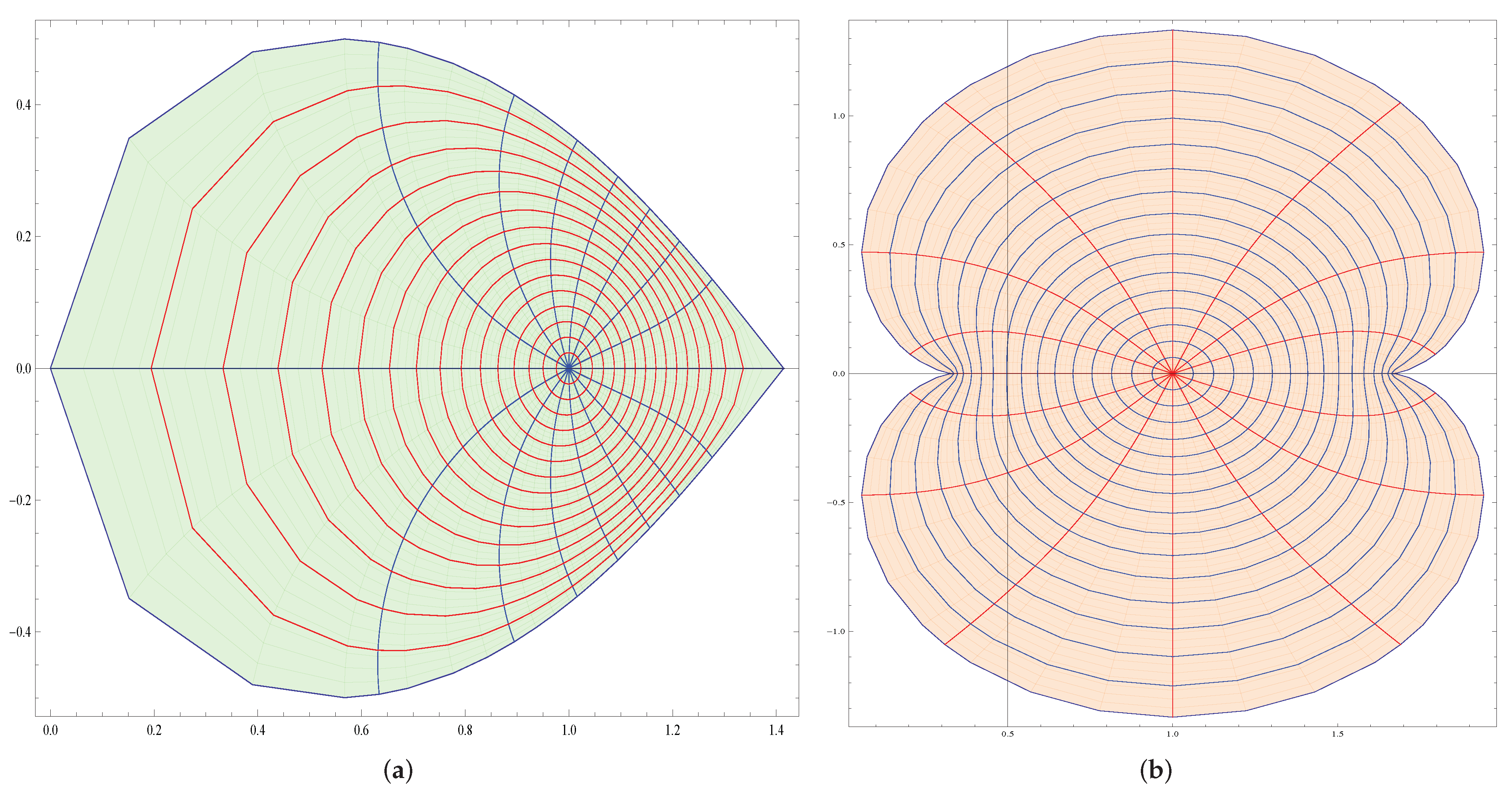
Mendiratta et al. in [41] defined a class of functions subordinate to

$$\Phi \left(z\right)=\sqrt{2}-(\sqrt{2}-1)\left(\sqrt{\frac{1-z}{1+2\left(\sqrt{2}-1\right)z}}\right).$$

The function $\Phi \left(z\right)=\sqrt{2}-\left(\sqrt{2}-1\right)\sqrt{\frac{1-z}{1+2\left(\sqrt{2}-1\right)z}}$ maps the unit disc onto interior of the left half of the shifted lemniscate of Bernoulli ${\left[{(u-\sqrt{2})}^2+v^2\right]}^2-\left[{(u-\sqrt{2})}^2+v^2\right]=0$ (see Figure 1a). The function $\Phi \left(z\right)$ has a Maclaurin series of the form

$$\Phi \left(z\right)=1+\left(\frac{5}{2}-\frac{3}{\sqrt{2}}\right)z+\left(\frac{71}{8}-\frac{51}{4\sqrt{2}}\right)z^2+\left(\frac{589}{16}-\frac{415}{8\sqrt{2}}\right)z^3+O{\left[z\right]}^4.$$

In [42], Wani and Swaminathan introduced and studied a class of functions subordinate to $\Phi \left(z\right)=1+z-z^3/3$. The function $\Phi \left(z\right)=1+z-z^3/3$ maps the unit disc onto a region bounded by the nephroid ${\left[{(u-1)}^2+v^2-\frac{4}{9}\right]}^2-\frac{4v^2}{3}=0$ (see Figure 1b), which is symmetric about the real axis.

If we let $m=\lambda =\theta =\beta =0$, $b=\delta =\rho =1$, $\Theta \left(z\right)=1$ and $\Phi \left(z\right)=\sqrt{2}-\left(\sqrt{2}-1\right)\sqrt{\frac{1-z}{1+2\left(\sqrt{2}-1\right)z}}$ in Theorem 5, we obtain

Corollary 8. 

If $f\left(z\right)\in {\mathcal{M}}_1$ satisfies the condition

$$-\frac{z{f}^{\prime }\left(z\right)}{f\left(z\right)}\prec \sqrt{2}-\left(\sqrt{2}-1\right)*\sqrt{\frac{1-z}{1+2\left(\sqrt{2}-1\right)z}},$$

then for all $\mu \in \mathbb{C}$ we have

$$\begin{array}{c}\left|a_1-\mu a_0^2\right|\le \frac{(5-3\sqrt{2})}{4}max\left\{1;\frac{6\sqrt{2}-7}{4}+\frac{5-3\sqrt{2}}{2}\left|2\mu -1\right|\right\}.\end{array}$$

The inequality is sharp for each $\mu \in \mathbb{C}$.

If we let $m=\lambda =\theta =\beta =0$, $b=\delta =\rho =1$, $\Theta \left(z\right)=1$ and $\Phi \left(z\right)=1+z-z^3/3$ in Theorem 5, we obtain

Corollary 9. 

If $f\left(z\right)\in {\mathcal{M}}_1$ satisfies the condition

$$-\frac{z{f}^{\prime }\left(z\right)}{f\left(z\right)}\prec 1+z-z^3/3,$$

then for all $\mu \in \mathbb{C}$ we have

$$\begin{array}{c}\left|a_1-\mu a_0^2\right|\le \frac{1}{2}max\left\{1;\frac{1}{3}+|2\mu -1|\right\}.\end{array}$$

The inequality is sharp for each $\mu \in \mathbb{C}$.

5. Discussion

As a preclude to the Conclusions section, in this section we will highlight the significance of our main results and their applications in detail. With a primary motive to consolidate the study of the famous $\alpha$-convex function with starlike and convex functions, Al-Oboudi in [43] defined an operator containing a convex combination of analytic functions. However, the same meromorophic analogue of the Al-Oboudi operator could not be defined to unify the meromorphic $\alpha$-convex function with other geometrically defined subclasses of ${\mathcal{M}}_p$. Aouf in [4] intelligently defined an Al-Oboudi-type operator for functions in ${\mathcal{M}}_p$ in such a way that normalization could be retained. In this paper, we extend the operator defined by Aouf in [4] by replacing f with $f*{\mathcal{K}}_{\theta ,\vartheta }^{\rho }\left(z\right)$, where * denotes the Hadamard product and ${\mathcal{K}}_{\theta ,\vartheta }^{\rho }\left(z\right)$ is the normalized meromorphic function with the Prahakar function in the kernel.

The family of functions ${\mathcal{KC}}_{\lambda }^m(\beta ,\rho ,\theta ,\vartheta ;b;\Phi )$ (see Definition 1) is defined to include or unify the study of $\delta$-pseudo starlike functions. Furthermore, to add more versatility to our study, we defined the class ${\mathcal{KC}}_{\lambda }^m(\beta ,\rho ,\theta ,\vartheta ;b;\Phi )$ by subjecting a certain analytic characterization quasi-subordinate to a more general function. The other class ${\mathcal{MB}}_{\lambda }^m(\rho ,\theta ,\vartheta ;b;\Phi )$ (see Definition 2) was defined to extend the study of Ghoos et al. [31].

The other significant deviation from previous studies is that we obtain conditions so that $\delta$-pseudo starlike functions are quasi-subordinate to a general function. Hence, if we let $\Theta \left(z\right)=1$, then our results in Section 3 will reduce to a subordination condition for starlikeness. The method to obtain the solution to the Fekete–Szegő problem of ${\mathcal{MB}}_{\lambda }^m(\rho ,\theta ,\vartheta ;b;\Phi )$ and ${\mathcal{KC}}_{\lambda }^m(\beta ,\rho ,\theta ,\vartheta ;b;\Phi )$ is the same as that employed by various authors. However, several new and classical results can be obtained as a special case of our main results.

6. Conclusions

The extension and unification of various well-known classes of functions were the main objective of this paper. We defined a new family of multivalent meromorphic functions of complex order using a differential operator, to unify the study of various classes of meromorphic functions. Inclusion relations, Fekete–Szegő inequalities and sufficient conditions for starlikeness for the defined function class were established.

References

- Goodman, A.W. Univalent Functions; Mariner Publishing Co., Inc.: Tampa, FL, USA, 1983; Volume I. [Google Scholar]
- Hayman, W.K. Multivalent Functions; Cambridge Tracts in Mathematics and Mathematical Physics, No. 48; Cambridge University Press: Cambridge, UK, 1958. [Google Scholar]
- Liu, J.-L.; Srivastava, H.M. A linear operator and associated families of meromorphically multivalent functions. J. Math. Anal. Appl. 2001, 259, 566–581. [Google Scholar] [CrossRef]
- Aouf, M.K. A class of meromorphic multivalent functions with positive coefficients. Taiwan. J. Math. 2008, 12, 2517–2533. [Google Scholar] [CrossRef]
- Aouf, M.K.; Seoudy, T.M. Some families of meromorphic p-valent functions involvinga new operator defined by generalized Mittag–Leffler function. J. Egypt. Math. Soc. 2018, 26, 406–411. [Google Scholar] [CrossRef] [Green Version]
- Murugusundaramoorthy, G.; Aouf, M.K. Families of meromorphic multivalent functions associated with the Dziok-Raina operator. Int. J. Anal. Appl. 2005, 2, 1–18. [Google Scholar]
- Liu, J.-L.; Srivastava, H.M. Classes of meromorphically multivalent functions associated with the generalized hypergeometric function. Math. Comput. Model. 2004, 39, 21–34. [Google Scholar] [CrossRef]
- Ayub, U.; Mubeen, S.; Abdeljawad, T.; Rahman, G.; Nisar, K.S. The new Mittag–Leffler function and its applications. J. Math. 2020, 2020, 2463782. [Google Scholar] [CrossRef]
- Gorenflo, R.; Kilbas, A.A.; Rogosin, S.V. On the generalized Mittag–Leffler type functions. Integral Transform. Spec. Funct. 1998, 7, 215–224. [Google Scholar] [CrossRef]
- Kilbas, A.A.; Srivastava, H.M.; Trujillo, J.J. Theory and Applications of Fractional Differential Equations; North-Holland Mathematics Studies 204; Elsevier Science B.V.: Amsterdam, The Netherlands, 2006. [Google Scholar]
- Purohit, S.D.; Kalla, S.L. A generalization of q-Mittag–Leffler function. Mat. Bilten 2011, 35, 15–26. [Google Scholar]
- Prabhakar, T.R. A singular integral equation with a generalized Mittag Leffler function in the kernel. Yokohama Math. J. 1971, 19, 7–15. [Google Scholar]
- Aldawish, I.; Ibrahim, R.W. Solvability of a New q-Differential Equation Related to q-Differential Inequality of a Special Type of Analytic Functions. Fractal Fract. 2021, 5, 228. [Google Scholar] [CrossRef]
- Selvaraj, C.; Karthikeyan, K.R. Some inclusion relationships for certain subclasses of meromorphic functions associated with a family of integral operators. Acta Math. Univ. Comen. (N.S.) 2009, 78, 245–254. [Google Scholar]
- Haji Mohd, M.; Darus, M. Fekete–Szegő problems for quasi-subordination classes. Abstr. Appl. Anal. 2012, 2012, 192956. [Google Scholar] [CrossRef] [Green Version]
- Robertson, M.S. Quasi-subordination and coefficient conjectures. Bull. Am. Math. Soc. 1970, 76, 1–9. [Google Scholar] [CrossRef] [Green Version]
- Altınkaya, S. Application of quasi-subordination for generalized Sakaguchi type functions. J. Complex Anal. 2017, 2017, 3780675. [Google Scholar] [CrossRef] [Green Version]
- Atshan, W.G.; Rahman, I.A.R.; Lupaş, A.A. Some results of new subclasses for bi-univalent functions using quasi-subordination. Symmetry 2021, 13, 1653. [Google Scholar] [CrossRef]
- Karthikeyan, K.R.; Murugusundaramoorthy, G.; Cho, N.E. Some inequalities on Bazilevič class of functions involving quasi-subordination. AIMS Math. 2021, 6, 7111–7124. [Google Scholar] [CrossRef]
- Ramachandran, C.; Soupramanien, T.; Sokół, J. The Fekete-Szegö functional associated with k-th root transformation using quasi-subordination. J. Anal. 2020, 28, 199–208. [Google Scholar] [CrossRef]
- Ramachandran, C.; Soupramanien, T.; Vanitha, T. Estimation of coefficient bounds for the subclasses of analytic functions associated with Chebyshev polynomial. J. Math. Comput. Sci. 2021, 11, 3232–3243. [Google Scholar]
- Mogra, M.L. Meromorphic multivalent functions with positive coefficients. I. Math. Jpn. 1990, 35, 1–11. [Google Scholar]
- Mogra, M.L. Meromorphic multivalent functions with positive coefficients. II. Math. Jpn. 1990, 35, 1089–1098. [Google Scholar]
- Uralegaddi, B.A.; Ganigi, M.D. Meromorphic multivalent functions with positive coefficients. Nepali Math. Sci. Rep. 1986, 11, 95–102. [Google Scholar]
- Aouf, M.K. On a class of meromorphic multivalent functions with positive coefficients. Math. Jpn. 1990, 35, 603–608. [Google Scholar] [CrossRef]
- Aouf, M.K. A generalization of meromorphic multivalent functions with positive coefficients. Math. Jpn. 1990, 35, 609–614. [Google Scholar]
- Srivastava, H.M.; Hossen, H.M.; Aouf, M.K. A unified presentation of some classes of meromorphically multivalent functions. Comput. Math. Appl. 1999, 38, 63–70. [Google Scholar] [CrossRef] [Green Version]
- Elrifai, E.A.; Darwish, H.E.; Ahmed, A.R. On certain subclasses of meromorphic functions associated with certain differential operators. Appl. Math. Lett. 2012, 25, 952–958. [Google Scholar] [CrossRef] [Green Version]
- Lashin, A.Y. On certain subclasses of meromorphic functions associated with certain integral operators. Comput. Math. Appl. 2010, 59, 524–531. [Google Scholar] [CrossRef] [Green Version]
- Arif, M.; Ahmad, B. New subfamily of meromorphic multivalent starlike functions in circular domain involving q-differential operator. Math. Slovaca 2018, 68, 1049–1056. [Google Scholar] [CrossRef]
- Ghoos Ali Shah, S.; Hussain, S.; Rasheed, A.; Shareef, Z.; Darus, M. Application of quasisubordination to certain classes of meromorphic functions. J. Funct. Spaces 2020, 2020, 4581926. [Google Scholar]
- Karthikeyan, K.R.; Murugusundaramoorthy, G.; Bulboacă, T. Properties of λ-pseudo-starlike functions of complex order defined by subordination. Axioms 2021, 10, 86. [Google Scholar] [CrossRef]
- Bulut, S.; Adegani, E.A.; Bulboacă, T. Majorization results for a general subclass of meromorphic multivalent functions. Politeh. Univ. Buchar. Sci. Bull. Ser. A Appl. Math. Phys. 2021, 83, 121–128. [Google Scholar]
- Bulboacă, T. Differential Subordinations and Superordinations; Recent Results; House of Science Book Publishing: Cluj-Napoca, Romania, 2005. [Google Scholar]
- Pommerenke, C. Univalent Functions; Vandenhoeck & Ruprecht: Göttingen, Germany, 1975. [Google Scholar]
- Ma, W.C.; Minda, D. A unified treatment of some special classes of univalent functions. In Lecture Notes Analysis, I, Proceedings of the Conference on Complex Analysis, Tianjin, China, 19–23 June 1992; International Press Inc.: Cambridge, MA, USA, 1992; pp. 157–169. [Google Scholar]
- Aouf, M.K. On a class of p-valent starlike functions of order α. Int. J. Math. Math. Sci. 1987, 10, 733–744. [Google Scholar] [CrossRef] [Green Version]
- Breaz, D.; Karthikeyan, K.R.; Senguttuvan, A. Multivalent Prestarlike Functions with Respect to Symmetric Points. Symmetry 2022, 14, 20. [Google Scholar] [CrossRef]
- Janowski, W. Some extremal problems for certain families of analytic functions I. Ann. Pol. Math. 1973, 10, 297–326. [Google Scholar] [CrossRef] [Green Version]
- Mohankumar, D.; Senguttuvan, A.; Karthikeyan, K.R.; Ganapathy Raman, R. Initial coefficient bounds and fekete-szego problem of pseudo-Bazilevič functions involving quasi-subordination. Adv. Dyn. Syst. Appl. 2021, 16, 767–777. [Google Scholar]
- Mendiratta, R.; Nagpal, S.; Ravichandran, V. A subclass of starlike functions associated with left-half of the lemniscate of Bernoulli. Int. J. Math. 2014, 25, 1450090. [Google Scholar] [CrossRef]
- Wani, L.A.; Swaminathan, A. Starlike and convex functions associated with a nephroid domain. Bull. Malays. Math. Sci. Soc. 2021, 44, 79–104. [Google Scholar] [CrossRef]
- Al-Oboudi, F.M. On univalent functions defined by a generalized Sălăgean operator. Int. J. Math. Math. Sci. 2004, 2004, 1429–1436. [Google Scholar] [CrossRef] [Green Version]
Figure 1.
(a) Mapping of under . (b) Mapping of under the transformation .
Publisher’s Note: MDPI stays neutral with regard to jurisdictional claims in published maps and institutional affiliations. |
© 2022 by the authors. Licensee MDPI, Basel, Switzerland. This article is an open access article distributed under the terms and conditions of the Creative Commons Attribution (CC BY) license (https://creativecommons.org/licenses/by/4.0/).
Share and Cite
MDPI and ACS Style
Breaz, D.; Karthikeyan, K.R.; Umadevi, E. Subclasses of Multivalent Meromorphic Functions with a Pole of Order p at the Origin. Mathematics 2022, 10, 600. https://0-doi-org.brum.beds.ac.uk/10.3390/math10040600
AMA Style
Breaz D, Karthikeyan KR, Umadevi E. Subclasses of Multivalent Meromorphic Functions with a Pole of Order p at the Origin. Mathematics. 2022; 10(4):600. https://0-doi-org.brum.beds.ac.uk/10.3390/math10040600
Chicago/Turabian StyleBreaz, Daniel, Kadhavoor R. Karthikeyan, and Elangho Umadevi. 2022. "Subclasses of Multivalent Meromorphic Functions with a Pole of Order p at the Origin" Mathematics 10, no. 4: 600. https://0-doi-org.brum.beds.ac.uk/10.3390/math10040600
Note that from the first issue of 2016, this journal uses article numbers instead of page numbers. See further details here.