Efficient Malware Classification by Binary Sequences with One-Dimensional Convolutional Neural Networks

Abstract

The rapid increase of malware attacks has become one of the main threats to computer security. Finding the best way to detect malware has become a critical task in cybersecurity. Previous work shows that machine learning approaches could be a solution to address this problem. Many proposed methods convert malware executables into grayscale images and apply convolutional neural networks (CNNs) for malware classification. However, converting malware executables into images could twist the one-dimensional structure of binary codes. To address this problem, we explore the bit and byte-level sequences from malware executables and propose efficient one-dimensional (1D) CNNs for the malware classification. Our experiments evaluate our proposed 1D CNN models with two benchmark datasets. Our proposed 1D CNN models achieve better performance from the experimental results than the existing 2D CNNs malware classification models by providing smaller resizing bit/byte-level sequences with less computational cost.

1. Introduction

Malware is software designed to damage computer networks and systems. The rapid increase of malware attacks has become one of the main threats to computer security. In addition to the scale of malware, recent reports also show that the malware variants have become more sophisticated [1]. Finding the best way to detect malware has become a critical task in cybersecurity. Many antivirus engines widely use signature-based detection for malware detection methods [2]. The signatures, such as particular patterns of byte code and text strings, are typically defined by the domain experts via inspecting malware instances. Once the signatures are determined, one can apply the pattern matching of the signatures to malware detection. However, the signature-based methods are not adaptive to the rapid changes of those malware variants since the signature matching can only detect malware that does not vary significantly.

Many machine learning approaches have been proposed to overcome these problems mentioned above [3,4,5,6,7]. Unlike the signature-based methods, machine learning approaches aim to build a data-driven model for malware detection based on defined features. There are typically two significant categories of malware analysis for feature extraction: static and dynamic methods [8,9,10]. The static analysis is conducted in a non-runtime environment, and the corresponding features could be extracted from executables by reverse engineering, such as byte-sequence and string features. For the dynamic analysis, one needs to run malware in an isolated environment to observe its behaviors and capture the malicious attacks. Based on static and dynamic analyses, domain experts could design valuable features of an executable for malware detection. Many feature extraction approaches have also been proposed for malware detection methods [9,10]. However, the process of extracting these manual features could be difficult, expensive, or time-consuming.

In addition to the features designed by domain experts, many works also used visual features in many malware detection methods [11,12,13,14,15,16,17]. More specifically, sequential chunks of binary executables are converted into two-dimensional grayscale images, as shown in Figure 1. Thus, we can represent each executable by visual features, such as SURF, GIST, and SIFT [11,18]. Once the visual features are extracted, many classic classification methods, such as support vector machines (SVM) or random forest, can be applied to classify the growing number of malicious executables. On the other hand, convolutional neural networks (CNNs) have achieved great success in computer vision, such as image classification and object detection. Similar to the applications in computer vision, CNNs can automatically extract the informative features by the learned filters. Many malware detection methods also have adopted CNNs as an end-to-end detector [12,13,16]. These works aim to classify malware executables acquired by binary executables into their corresponding families [19,20,21,22]. Unlike these CNN-based methods, we proposed one-dimensional convolutional neural networks to learn the features from raw binary sequences for the malware classification. That is, we designed a simple architecture of one-dimensional CNN in our proposed method by considering the structure of binary sequences from executables. In our experiments, we also compare traditional machine learning algorithms and other proposed deep learning algorithms [11,12,13,14,15,16,17] to evaluate the performance of our proposed method. In addition to converting malicious programs to images for classification, compressing images or binary sequences is also a key factor for the results. The lower the degree of compression, the more virus codes information maintained in an image or binary sequence. Thus, we also studied the influence of different resized images in our work. The main contributions of this work are listed as follows:

• We proposed a byte-level 1D CNN model to explore informative features from the one-dimensional structure of binary executables. The experimental results show that our 1D CNN model could achieve promising results by giving smaller resizing bit/byte-level sequences.
• In addition to the byte-level 1D CNN model, we also proposed a bit-level 1D CNN mode by expanding bytes into bits from byte sequences. Our experiments show that we could augment the information from the byte sequences with the bit expansion to achieve better performance.
• Our proposed 1D CNNs achieve better or comparable results with less computational cost compared with 2D CNNs in terms of the amount of multiply-add operations.
• Our experiments present comprehensive experimental results of applying different resizing lengths for 1D and 2D CNN models. The results could provide a guideline for considering different resizing lengths for CNN-based malware classification methods in the future.

The rest of this paper is organized as follows. In Section 2, we briefly review the related work on malware detection. Section 3 introduced our deep learning architecture and framework for malware classification. We discuss experimental results with various methods in Section 4. Finally, Section 5 concludes our work and addresses several feature works.

2. Related Work

In conventional machine learning approaches, one must define valuable features for the tasks. Domain experts could extract these features from static and dynamic analysis [9,23]. For example, Reference [23] defined the static features, such as function length frequency and printable string information. For the dynamic features, the authors extracted API features after running all the executable files and logging the Windows API calls. The number of occurrences of API features is encoded as a dynamic feature vector. Once the integrated static and dynamic features are obtained, classic classifiers, such as SVM and random forest, are applied for the malware classification. In [9], the authors also extract static and dynamic features from Android devices, such as instruction sequences and system call sequences. Rather than directly use the extracted features, the authors apply a deep auto-encoder to learn and combine new features for classification.

On the other hand, many works have focused on converting binary executables into images. For example, Reference [14] group binaries sequences of executables by 8-bit vectors. The transformed 8-bit vectors are then converted as grayscale images. After the process of conversion, Reference [14] directly applies random forest for malware classification by using pixel values as the features. In [11], the authors extract the visual features by classic computer vision feature extractors. For example, Reference [11] uses the GIST algorithm [24] to extract the characteristics of images and applied k-nearest neighbors for the malware classification. The results also show the improved performance by using these visual features. However, the classic visual features are designed for conventional image applications. These general-purpose features might not be suitable for malware classification. Besides, it also has been shown that it takes a large amount of memory space to search GIST features from an image dataset. Thus, some conventional visual features might not apply to malware classification since many large malicious programs are often produced in practice.

Recently, convolutional neural networks (CNNs) have shown powerful feature learning for image classification [25,26,27]. Many CNN-based approaches have been proposed for malware classification based on the conversion from binary executables to images [12,13,15,16,17,28,29,30,31]. Reference [17] applied different deep learning models, such as CNNs and GRUs, to classify malware families. The authors also applied LeakyReLU activation function and L2-SVM loss in their proposed methods. In [13], the authors compare their proposed CNN-based methods with conventional machine learning approaches. They show that malware classification methods based on CNNs can perform better than machine learning-based methods since appropriate features can be automatically learned. In [12], image-based malware classification using fine-tuned CNNs (IMCFN) is proposed. Unlike other CNN-based approaches, IMCFN converts raw malware binaries into color images. Rather than train CNNs from scratch, the authors use a pre-trained model with the ImageNet dataset. Moreover, data augmentation is also applied to handle the imbalance problem in malware classification. In [18], android malware detection experts studied APK files from different entry points. The authors convert binary data to RGB images or take the fragment data (input size: 512, 1024, 2048, 4096) for classification based on CNNs. In [32], the authors adopt the ResNet-like network with Bi-LSTM and attention mechanism to improve the performance of the detection method. MCFT-CNN [33] enhances the ResNet model by altering the last layer with a fully connected dense layer. MCFT-CNN model also has used transfer deep learning approaches from the natural image dataset.

Unlike previous works mentioned above, we proposed a simple architecture of one-dimensional CNN to classify malware executables. We directly use the sequences of binary executables with bit and byte levels. The one-dimensional structure keeps a program’s characteristics and avoids destroying the overall architecture of the malware executables. Our experiments show that our proposed methods improved the performance of the malware classification with much smaller resizing bit/byte-level sequences by comparing with 2D CNNs.

3. Malware Detection via Convolution Neural Networks

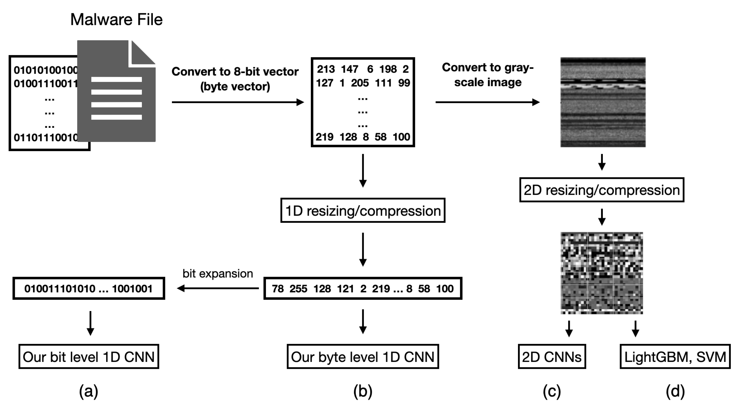
Typically, a program can be represented by different levels of representation, such as the assembly language or machine codes. Our work focuses on the machine codes: a binary sequence. These elements of one and zero can be regarded as the language of a computer system. Transforming these binary sequences into informative representations for malware classification is the most critical task in our work. By leveraging the powerful feature learning of CNNs, we aim to learn informative features from the binary executables. More specifically, there are two strategies to process binary executables, as shown in Figure 1. For the first one, i.e., Figure 1c,d, we convert the binary sequences into grayscale images and apply 2D CNNs to classify malware executables. Our second strategy is to directly apply 1D CNNs to the raw binary sequences with bit and byte levels, as shown in Figure 1a,b. Our work aims to automatically learn informative features from these unstructured data for malware detection. The details will be addressed in the following sections.

3.1. Malware Detection with 2D CNNs

The malicious files are constantly modified to avoid detection from rule-based models in malware detection. The obfuscation with various tactics also leads to detection difficulties. Previous work has studied malware by static analysis, such as assembly language or binary codes. However, the binary codes are only composed of zeros and ones. It is not easy to extract informative features or clues for malware classification. To overcome this problem, malware experts use visualization tools to analyze the structure of the binary codes and extract the features. Compared with the features extracted from domain knowledge, visual features can be extracted from malware images for malware classification.

In addition to the conventional visual features, such as SURF, GIST, and SIFT, CNNs can improve accuracy and efficiency by automatic feature learning [11,18]. In our first framework for malware detection, we apply conventional two-dimensional CNNs (2D CNNs) to learn the informative features from these converted images, as shown in Figure 1c. More specifically, we re-encode the binary data with an 8-bit converter. Every 8-bit segment is converted to the intensity of grayscale. It is worth noting that the sizes of converted images are often huge since the machine codes of executables are also large. Thus, we apply compression methods and resize the image to the proper size. More specifically, we resize the malware images to different sizes, such as 32 × 32, 48 × 48, 64 × 64, and 128 × 128, in our experiments. The comparisons of different resizing sizes will be addressed in our experiments. After the preprocessing, we adopt VGGNet [25], ResNet [27], and EfficientNet [34] as our 2D CNNs for malware detection.

VGGNet is proposed to explore how the depth of convolutional neural networks affects the accuracy of large-scale image classification and recognition. To balance the depth of neural networks and excessive parameters, 3 × 3 convolutional layers are used in all layers, and the step size is set to 1. There are five convolution blocks VGGNet, and each convolution block has 2 to 3 convolutional layers. It has been shown that the receptive field of two 3 × 3 convolutions has the same effect as a 5 × 5 convolution; three 3 × 3 convolutions linked together have the same effect as a 7 × 7 convolution. In addition, the three series of 3 × 3 convolutions have fewer parameters than a 7 × 7 convolution. Most importantly, the three 3 × 3 convolutions have more nonlinear transformations than a 7 × 7 convolution. It makes the model more capable of learning features. After that, each convolution block is connected to a max-pooling layer to reduce the size of the image.

ResNet [27] is proposed to address the problem of degradation while the depth of the neural network is increasing. ResNet is equivalent to changing the learning target. ResNet aims to fit the residuals rather than directly learn the mapping between the input and output. The entire network only needs to focus on learning the residuals, simplifying the learning objectives and difficulties. Besides, the projection shortcut in ResNet also avoids the excessive parameters used in the networks. EfficientNet [34] uses neural architecture search to design a new baseline network and scale it up to obtain a family of models (EfficientNet-B0 to EfficientNet-B7). Our experiments adopt EfficientNet-B0 to learn the malware classification models with the malware images. FractalNet [35] introduce a design strategy for neural network macro architecture based on self-similarity. The proposed networks contain interacting subpaths of different lengths but do not include any pass-through or residual connections. A filter and nonlinearity transform every internal signal before being seen by subsequent layers.

3.2. Malware Detection by 1D CNNs with Byte-Level Sequences

As described in Section 3.1, a malware executable is represented by a binary sequence and converted into an image. That is, a sequential machine code is converted into a 2-dimensional structure. However, the 2-dimensional conversion could twist the sequential structure of the machine codes since a fixed width will cut the sequential binary codes. More specifically, the binary codes representing a certain behavior might be broken into pieces because the image’s width must be determined. For example, assume that mov eax in assembly language is compiled as 8B C6 in machine code. 8B C6 could be split into different rows in the converted image, and the structure of mov eax will not be maintained. Besides, different widths of the conversion will represent different 2-dimensional structures for the same malware image. It is difficult to determine a fixed width that can maintain all inherited sequential structures within the binary codes.

Rather than convert the malware executables into images, we aim to apply one-dimensional CNNs to the binary codes for maintaining the sequential structures. In our proposed methods, we represent malware executables with different levels of sequences. The first one is the byte-level sequences, as shown in Figure 1b. We encode each 8-bit sequence into bytes to represent malware executables by byte-level sequences. However, the length of a byte sequence from a malware executable could be extremely large. Besides, different lengths of binary executables are not easy to apply for CNNs. Similar to converting malware executables as images, we also apply resizing or compression methods to fix the length of each byte-level sequence. We resize each byte-level executable to different lengths in our framework, including 1 × 1024, 1 × 2304, 1 × 4096, and 1 × 16,384. These different lengths correspond to the 32 × 32, 48 × 48, 64 × 64, and 128 × 128 malware images for the 2D CNNs. Once each binary executable is preprocessed, we apply these data to train our proposed byte-level malware classification model with the one-dimensional CNN.

In our proposed byte-level 1D CNN model for malware classification, there are five/six convolution blocks in the architecture, as shown in

Table 1. The network structure of our proposed byte-level 1D CNN for malware classification. The number after the @ symbol represents the size of channels produced by the convolution. The s and p represent the stride and the padding, respectively.

Input: 1 × 1 × 1024	Input: 1 × 1 × 2304	Input: 1 × 1 × 4096	Input: 1 × 1 × 16,384
-	-	-	kernel: 1 × 8 @16
			s: 8, p: 0
kernel: 1 × 3 @16	kernel: 1 × 3 @16	kernel: 1 × 3 @16	kernel: 1 × 3 @16
s: 1, p: 1	s: 2, p: 1	s: 2, p: 1	s: 1, p: 1
LeakyReLU	LeakyReLU	LeakyReLU	LeakyReLU
Max Pooling: 1 × 2
kernel: 1 × 3 @32
s: 2, p: 1
LeakyReLU
Max Pooling: 1 × 2
kernel: 1 × 3 @64	kernel: 1 × 3 @64	kernel: 1 × 3 @64	kernel: 1 × 3 @64
s: 1, p: 1	s: 1, p: 1	s: 2, p: 1	s: 2, p: 1
LeakyReLU	LeakyReLU	LeakyReLU	LeakyReLU
Max Pooling: 1 × 2
kernel: 1 × 3 @128
s: 2, p: 1
LeakyReLU
Max Pooling: 1 × 2
kernel: 1 × 3 @128
s: 2, p: 1
LeakyReLU
FC: 512
LeakyReLU
FC: class size
Softmax

. Most convolution blocks contain 1 × 3 convolution layers with the LeakyReLU activation function. The length of the convoluted sequences can be determined as follows:

$$L_{out}=\lfloor \frac{L_{in}+2\times padding-dilation\times (kernel\_size-1)-1}{stride}+1\rfloor ,$$

(1)

where $L_{in}$ and $L_{out}$ represent the lengths of sequences before and after the convolution, respectively. Similar to the conventional CNNs, we also apply the max-pooling layer after the convolution blocks. We add an extra 1 × 8 convolution layer with eight-striding and zero-padding for resizing 1 × 1 × 16,384 inputs, compared to other input sizes. The 1 × 8 convolution layer will dramatically reduce the size of inputs from 1 × 1 × 16,384 to 1 × 1 × 2048. After the final convolution block, we did not apply the max-pooling layer since we kept the most information from the one-dimensional features before forwarding it to the fully-connected layers. We aggregate all the convoluted sequences into a 512-dimensional vector in our fully-connected layer. Our proposed model uses two fully connected layers and the softmax layer with cross-entropy loss followed by the convolution blocks.

3.3. Malware Detection by 1D CNNs with Bit-Level Sequences

In addition to byte-level sequences, we also represent malware executables by the bit-level sequences. As mentioned in the strategy of adopting the byte-level sequence, we also resize the sequence to a fixed length. This resizing could be viewed as data compression. Rather than compress bit-level sequences directly, we first encode each 8-bit sequence into bytes by the same trick in converting byte-level sequences into malware images. Once the resizing byte-level sequences are obtained, we apply the bit transformation to expand them to bit-level sequences. This is because each machine instruction is encoded as 8 bits. Resizing the bit-level sequences directly twists the structure of the machine instruction. For example, as shown in

Table 2. The network structure of our proposed bit-level 1D CNN for malware classification. The number after the @ symbol represents the size of channels produced by the convolution. The s and p represent the stride and the padding, respectively.

Input: 1 × 1 × 1024	Input: 1 × 1 × 2304
bit expansion (byte to bit)
1 × 1 × 8192	1 × 1 × 18,432
kernel: 1 × 8 @16
s: 8, p: 0
kernel: 1 × 3 @16
s: 1, p: 1
LeakyReLU
Max Pooling: 1 × 2
kernel: 1 × 3 @32
s: 2, p: 1
LeakyReLU
Max Pooling: 1 × 2
kernel: 1 × 3 @64	kernel: 1 × 3 @64
s: 1, p: 1	s: 2, p: 1
LeakyReLU	LeakyReLU
Max Pooling: 1 × 2
kernel: 1 × 3 @128
s: 2 p: 1
LeakyReLU
Max Pooling: 1 × 2
kernel: 1 × 3 @128
s: 2, p: 1
LeakyReLU
FC: 512
LeakyReLU
FC: class size
Softmax

, we first apply the bit-to-byte transformation, resize the length of the byte-level sequences by 1 × 1024, and apply the bit expansion to obtain the 1 × 8192 bit-level sequences.

Similar to our proposed byte-level one-dimensional CNN, our bit-level one also adopts a similar architecture. There are six convolution blocks and two fully-connected layers in our bit-level 1D CNN model. We aim to determine kernel size and striding length with explainable values for the first convolution block rather than search these hyperparameters by the grid search approach. More specifically, we set it by eight to determine the kernel size since each machine instruction is encoded as 8 bits. Since it is the same in determining kernel size, the striding length is also set by eight due to the non-overlapping executing of machine executing. We adopt similar structures for the remainder convolution blocks as in our byte-level 1D CNN model. The lengths of the convoluted sequences can also be calculated with (1). In our experiments, byte-level and bit-level 1D CNN models are used for evaluation. The details are discussed in Section 4.

Compared to using malware images in Section 3.1, our proposed bit/byte-level 1D CNNs maintain the contextual information for the machine codes or instructions. Besides, the number of parameters required by our proposed 1D CNNs is much less than using 2D CNNs, such as VGGNet. Our experiments show that our proposed 1D CNN improves the accuracy of the malware classification while giving smaller resizing bit/byte-level sequences.

4. Experiments

4.1. Experimental Setting

Our experiments compare our proposed 1D CNNs with 2D CNNs and conventional machine learning approaches. As noted in Section 3.1, VGG-16, RestNet-18, and EfficientNet-B0 are included in our experiments to evaluate the effectiveness of 2D CNNs for malware classification. In addition to these popular CNN models, existing malware classification methods with visual features, such as [11,12,13,16,33], are also included in our experiments. Compared with conventional machine learning approaches, we select Decision Tree, SVM [17,36], Random Forest [14,37], and LightGBM [38] in our experiments.

We have two resizing strategies for 1D and 2D CNN models in our data preprocessing. As shown in Figure 1, we will first convert the binary executables into 8-bit vectors. We apply 2D nearest neighbors image resizing for all 2D CNN models and conventional machine learning approaches following the conversion. Unlike the 2D CNN models, we apply 1D nearest neighbors resizing for the byte-sequences. Once the resized byte-level sequences are obtained, we then apply the bit expansion for generating the bit-level sequences. Our experiments convert the binary executables into 32 × 32, 48 × 48, 64 × 64, and 128 × 128 malware images for all 2D CNN models. We also flatten them into one-dimensional arrays as the input of the conventional machine learning approaches. On the other hand, we convert the binary executables into 1 × 1024, 1 × 2304, 1 × 4096, and 1 × 16,384 byte-level sequences for our byte-level 1D CNN model. Among these different lengths of byte-sequences, we apply the bit expansion to 1 × 1024 and 1 × 2304 byte-level sequences and obtain 1 × 8192 and 1 × 18,432 byte-level sequences for our bit-level 1D CNN models.

We evaluate all the malware classification models with two real-world malware datasets by the accuracy. One is from Microsoft Malware Classification Challenge [39,40]. This dataset contains 10,868 instances and nine malware families as the training set in the contest. The other one is the Malimg dataset. There are 9339 instances and 25 malware families in this dataset. Our experiments split these datasets into a training set (80%), validation set (10%), and testing set (10%), respectively. The validation set is used to determine the optimal checkpoint during the training process. Once the optimal checkpoint is obtained, we apply the learned model to testing data to calculate the testing accuracy. To test the robustness of all the models, we repeat the random splits 10 times and report the averaged accuracy and the corresponding standard deviation.

For the implementation, VGG-16, RestNet-18, and EfficientNet-B0 are directly imported from the torchvision package of Pytorch. Our 1D CNN models are also implemented with Pytorch on our own. We train all the CNN modes with 100 epochs under the SGD optimizer where the learning rate and the momentum are 0.01 and 0.9, respectively. All the experiments are conducted with P100 GPU, 24 GB memory, and two vCPU. The detailed experimental results are also presented in Section 3 and Section 4.3.

4.2. Microsoft Malware Classification Challenge Dataset

Microsoft Malware Classification Challenge [39,40] is a competition held by Microsoft in Kaggle. The dataset contains 10,868 samples from nine different malware families, as shown in

Table 3. Data description of Microsoft Malware Classification Challenge (BIG 2015).

Label	Malware Family	Size
0	Ramnit	1541
1	Lollipop	2478
2	Kelihos_ver3	2942
3	Vundo	475
4	Simda	42
5	Tracur	751
6	Kelihos_ver1	398
7	Obfuscator. ACY	1228
8	Gatak	1013

. Each malware sample has two files as the raw presentation. The .bytes file contains the hexadecimal representation without the executable headers. On the other hand, the .asm file contains the code extracted by the IDA disassembler tool. We only use the .bytes files as the data instances in our experiments. These binary-coded files are converted into images and one-dimensional binary sequences, as described in Section 3.

For the evaluation, the results of conventional machine learning approaches with flattened raw features are presented in the first four rows of

Table 4. The reported accuracies of Microsoft Malware Classification Challenge dataset.

	Length of Resizing Executables (Bytes)
Method	32 × 32 (1 × 1024)	48 × 48 (1 × 2304)	64 × 64 (1 × 4096)	128 × 128 (1 × 16,384)
Decision Tree	0.7037 ± 0.0077	0.7050 ± 0.0089	0.7121 ± 0.0117	0.7173 ± 0.0149
SVM	0.8372 ± 0.0115	0.8439 ± 0.0111	0.8527 ± 0.0111	0.8541 ± 0.0138
Random Forest	0.8252 ± 0.0078	0.8277 ± 0.0118	0.8336 ± 0.0080	0.8375 ± 0.0070
LightGBM	0.8745 ± 0.0070	0.8778 ± 0.0065	0.8797 ± 0.0085	0.8813 ± 0.0078
VGG-16	0.9235 ± 0.0060	0.9404 ± 0.0095	0.9522 ± 0.0082	0.9666 ± 0.0059
ResNet-18	0.9011 ± 0.0088	0.9330 ± 0.0088	0.9463 ± 0.0065	0.9700 ± 0.0070
EfficientNet-B0	0.9091 ± 0.0048	0.9449 ± 0.0063	0.9589 ± 0.0060	0.9736 ± 0.0055
FractalNet	0.9456 ± 0.0068	0.9552 ± 0.0073	0.9583 ± 0.0083	0.9596 ± 0.0088
Ours (byte)	0.9244 ± 0.0083	0.9458 ± 0.0075	0.9542 ± 0.0085	0.9629 ± 0.0063
Ours (bit)	0.9549 ± 0.0055	0.9632 ± 0.0078	-	-

. The results show that the ensemble methods, such as random forest and LightGBM, could better perform these conventional machine learning approaches. The results also indicate that using flattened raw features might need more complicated models for the malware classification.

In addition to the results of using flattened raw features, the results of applying 2D CNNs and our proposed 1D CNNs are also shown in Table 4. The results of 2D CNNs show that 2D CNNs with malware images could achieve better performance through comparison with the conventional machine learning approaches. In our experiments, we also consider different lengths of resizing images as shown in Table 4. From the results, the retained information of 128 × 128 images is richer than others, and the best-improved performance can be achieved among all the different resized images. However, larger images require more computational cost and memory space. It is worth noting that we only experiment with the 128 × 128 images due to the limits of the device capability. Similar to other computer vision tasks, these popular CNN architectures benefit the malware classification. Of course, as with increasing image size, more complicated models also require a more computational cost.

From the results of Table 4, our proposed byte/bit-level 1D CNNs achieve better performance through comparison with 2D CNNs, while giving smaller resizing bit/byte-level sequences. For example, our bit-level 1D CNN model can achieve 0.9549 accuracies with 1 × 1024 byte sequences, whereas the 2D CNN models can only achieve 0.9235 accuracies at most. This shows that considering the 1D structure in the binary codes benefits malware classification, especially for a given smaller resizing sequence. It is worth noting that our proposed models did not outperform 2D CNNs for large resizing images. The reason could be that larger images might need a more complicated model for the learning task. However, in our 1D CNN model, only a simple architecture is designed for the learning task. Besides, we also found that our bit-level model achieves better performance by comparing the byte-level model under the exact size of byte sequences, although the byte-level 1D CNN requires less computation cost. The results also indicate that bit expansion for the byte sequences is a proper strategy for analyzing binary executables.

In addition to reporting accuracy, we also calculate the amount of multiply–accumulate (MAC) operations for all CNN models. All the amounts of MAC operations are presented by million units in

Table 5. The number of multiply–accumulate (MAC) operations of convolutional neural networks in our experiments.

	32 × 32 (1 × 1024)	48 × 48 (1 × 2304)	64 × 64 (1 × 4096)	128 × 128 (1 × 16,384)
Method	the Amount of MAC Operations (million Units)
VGG-16	442.35	823.22	1370.43	5112.78
ResNet-18	35.58	94.74	142.29	569.15
EfficientNet-B0	8.66	23.20	32.65	128.57
FractalNet	843.56	1898.00	3374.26	13,497.04
Ours (byte)	3.05	3.43	3.57	5.34
Ours (bit)	3.94	6.01	-	-

. As shown in Table 5, our proposed 1D CNN architectures learn the recognition models efficiently. For 1 × 1024 (32 × 32) and 1 × 2304 (48 × 48) input sizes, our proposed 1D CNN models not only achieve better accuracy but also require fewer MAC operations. On the other hand, our proposed methods only achieve comparable performance for 1 × 4096 (64 × 64) and 1 × 16,384 (128 × 128) input sizes. However, our proposed 1D CNN models require much fewer MAC operations for learning the classification model, especially for the 1 × 16,384 (128 × 128) input size. From Table 4 and Table 5, the results show that our proposed 1D CNNs are effective both in classification ability and computational cost.

4.3. Malimg Dataset

Malimg dataset is a public malware classification benchmark dataset in Kaggle. This dataset contains 9435 malware executables collected from 25 malware families, as shown in

Table 6. Data description of Malimg Dataset.

Label	Malware Family	Size	Label	Malware Family	Size
0	Lolyda. AT	159	13	Swizzot.gen!E	128
1	VB.AT	408	14	Swizzot.gen!I	132
2	Skintrim. N	80	15	Malex.gen!J	136
3	Lolyda. AA 2	184	16	Rbot!gen	158
4	Dialplatform. B	177	17	C2Lop.gen!G	200
5	Obfuscator. AD	142	18	Adialer. C	122
6	Agent. FYI	116	19	Yuner. A	800
7	Lolyda. AA 1	213	20	Wintrim. BX	97
8	Allaple. A	2949	21	Instantaccess	431
9	Allaple. L	1591	22	Autorun. K	106
10	Lolyda. AA 3	123	23	Dontovo. A	162
11	C2Lop. P	146	24	Fakerean	381
12	Alueron.gen!J	198

. However, the malware executables have been converted to 32 × 32 images using the nearest neighbor interpolation from Kaggle website. We visited the Vision Research Lab website (https://vision.ece.ucsb.edu/research/signal-processing-malware-analysis, accessed on 14 February 2022) to get the original converted images and download the images before compressed. With these original images, we can further flatten them to one-dimensional binary sequences for our proposed 1D CNNs.

For the first experiment with the Malimg dataset, we also apply conventional machine learning approaches with flattened raw features. The results are presented in

Table 7. The reported accuracies of Malimg Dataset.

	Length of Resizing Executables (Bytes)
Method	32 × 32 (1 × 1024)	48 × 48 (1 × 2304)	64 × 64 (1 × 4096)	128 × 128 (1 × 16,384)
Decision Tree	0.7990 ± 0.0136	0.9260 ± 0.0072	0.9257 ± 0.0068	0.9416 ± 0.0069
SVM	0.8471 ± 0.0086	0.9434 ± 0.0079	0.9461 ± 0.0060	0.9605 ± 0.0056
Random Forest	0.8557 ± 0.0079	0.9586 ± 0.0062	0.9605 ± 0.0054	0.9716 ± 0.0041
LightGBM	0.8638 ± 0.0070	0.9606 ± 0.0062	0.9591 ± 0.0049	0.9667 ± 0.0043
VGG-16	0.9198 ± 0.0164	0.9677 ± 0.0084	0.9815 ± 0.0042	0.9872 ± 0.0030
ResNet-18	0.8499 ± 0.0132	0.9564 ± 0.0062	0.9752 ± 0.0041	0.9810 ± 0.0044
EfficientNet-B0	0.8448 ± 0.0112	0.9617 ± 0.0066	0.9785 ± 0.0037	0.9852 ± 0.0031
FractalNet	0.9537 ± 0.0059	0.9714 ± 0.0063	0.9829 ± 0.0035	0.9841 ± 0.0039
Ours (byte)	0.9695 ± 0.0033	0.9777 ± 0.0046	0.9837 ± 0.0024	0.9891 ± 0.0022
Ours (bit)	0.9847 ± 0.0041	0.9870 ± 0.0040	-	-

. Similar to the Microsoft Malware Classification Challenge dataset results, Random Forest and LightGBM achieve the best performance compared with other conventional machine learning approaches. In the second experiment with the Malimg dataset, we also present the results of applying 2D CNNs and our proposed 1D CNNs in Table 7. From the results of applying 2D CNNs, all 2D CNN models outperform conventional machine learning approaches that directly use grayscales as features under different lengths of resizing. The results again show that feature learning via convolutional networks benefits malware classification with visual features. Among CNN models, our proposed bit-level 1D CNN achieves the best performance for malware classification compared with 2D CNNs under resizing lengths 1 × 1024 and 1 × 2304. The proposed byte-level 1D CNN also achieves better performance for the resizing lengths of 1 × 4096 and 1 × 16,384. Similar to the Microsoft Malware Classification Challenge dataset results, learning features from the 1D structure in the binary codes is a more appropriate feature extraction for malware classification.

In our final experiment with Malimg dataset, we compare our proposed 1D CNNs to other existing malware classification methods, including GIST + KNN [11], 2D CNN [16], M-CNN [13], IMCFN [12], and MCFT-CNN [33], as shown in

Table 8. The comparison to existing 2D CNN methods with our proposed bit-level 1D CNN for Malimg dataset.

Method	Resizing	Accuracy
GIST+KNN [11]	original images	0.9718
2D CNN [16]	128 × 128	0.9800
M-CNN [13]	224 × 224	0.9852
IMCFN [12]	224 × 224	0.9882
MCFT-CNN [33]	224 × 224	0.9918
Ours (byte)	1 × 16,384	0.9891 ± 0.0022
Ours (bit)	1 × 2304	0.9870 ± 0.0040

. GIST + KNN extracts the conventional visual features of images and applies k-nearest neighbors for classification. However, the classic visual features are designed for conventional image applications. These general-purpose features might not be suitable for malware classification. In the 2D CNN [16], all images are resized to 128 × 128 and a simple structure of convolutional networks is used. The results also show that features learned from the target domain data benefit the target task. M-CNN [13] resizes the images to 224 × 224; uses more complicated structures, such as VGGNet; and achieves better performance by comparing with 2D CNN [16]. In [12], IMCFN converts the raw malware binaries into 224 × 224 color images. Rather than train CNNs from scratch, the authors use a pre-trained model with the ImageNet dataset and achieve 0.9882 accuracies. MCFT-CNN [33] enhances the ResNet model by altering the last layer with a fully connected dense layer and achieving the best performance among 2D CNN models. Through comparison with the existing 2D CNN model in Table 8, our proposed 1D CNN models can produce comparable results among these existing methods by giving smaller resizing bit/byte-level sequences. The key difference is whether the 1D structure is adopted or not. The results also show that utilizing the 1D structure from binary executables to learn the features is more appropriate for malware classification.

4.4. Discussion

From the experiments of the Microsoft Malware Classification Challenge dataset and Malimg dataset, we show that, by converting the malware executables into malware images or byte sequences, the CNN-based models could automatically learn the informative features and classify the malware families without feature engineering and prior knowledge of binary code analysis or reverse engineering. We also found that the bit-level 1D CNN model could achieve very promising results for the smaller resizing bit/byte sequences. This also implies that we can learn the CNN models more efficiently since only smaller resizing bit/byte sequences are required.

The key difference between 1D CNN and 2D CNN models is that we explore the informative features by following the original one-dimensional structure of binary executables. Forcing the one-dimensional binary executables into a 2D image could twist the original information from the binary executables. Our proposed method did not always produce better performance while binary executables were converting and resizing to larger images, such as 128 × 128. The reason could be that larger images might need a more complicated model, such as ResNet or EfficientNet, for learning the informative features. However, in our 1D CNN models, only a simple architecture is designed for the learning task since the primary goal of our work is to show the effectiveness of considering one-dimensional sequences for malware classification.

5. Conclusions

In this work, we present 1D CNN models to classify malware executables. Rather than convert malware executables into images CNNs, our 1D CNN models explore the bit and byte-level sequences and learn the features automatically from malware executables. Our experiments show that our bit-level 1D CNN model can achieve 0.9632 and 0.9870 accuracies only 1 × 2304 byte sequences with bit expansion are given. Compared with these existing 2D CNN malware classification models, our proposed 1D CNN models achieve the highest accuracy with smaller resizing byte sequences and comparable accuracies with larger resizing byte sequences in Microsoft Malware Classification Challenge Malimg datasets. The results indicate that considering one-dimensional sequences will benefit the malware classification—not only the classification ability but also the computational cost.

References

- Malware Statistics and Facts. Available online: https://www.comparitech.com/antivirus/malware-statistics-facts/ (accessed on 14 February 2022).
- Schultz, M.G.; Eskin, E.; Zadok, F.; Stolfo, S.J. Data mining methods for detection of new malicious executables. In Proceedings of the 2001 IEEE Symposium on Security and Privacy, Oakland, CA, USA, 14–16 May 2001. [Google Scholar]
- Dahl, G.E.; Stokes, J.W.; Deng, L.; Yu, D. Large-scale malware classification using random projections and neural networks. In Proceedings of the 2013 IEEE International Conference on Acoustics, Speech and Signal Processing, Vancouver, BC, Canada, 26–31 May 2013. [Google Scholar]
- Saxe, J.; Berlin, K. Deep neural network based malware detection using two dimensional binary program features. In Proceedings of the 2015 10th International Conference on Malicious and Unwanted Software (MALWARE), Fajardo, PR, USA, 20–22 October 2015. [Google Scholar]
- Kolosnjaji, B.; Zarras, A.; Webster, G.; Eckert, C. Deep learning for classification of malware system call sequences. In Proceedings of the Australasian Joint Conference on Artificial Intelligence, Hobart, Tasmania, 5–8 December 2016. [Google Scholar]
- Yan, J.; Qi, Y.; Rao, Q. Detecting malware with an ensemble method based on deep neural network. Secur. Commun. Netw. 2018. [Google Scholar] [CrossRef] [Green Version]
- Hasegawa, C.; Iyatomi, H. One-dimensional convolutional neural networks for Android malware detection. In Proceedings of the 2018 IEEE 14th International Colloquium on Signal Processing & Its Applications (CSPA), Penang, Malaysia, 9–10 March 2018. [Google Scholar]
- Damodaran, A.; Di Troia, F.; Visaggio, C.A.; Austin, T.H.; Stamp, M. A comparison of static, dynamic, and hybrid analysis for malware detection. J. Comput. Virol. Hacking Tech. 2017, 13, 1–12. [Google Scholar] [CrossRef]
- Xu, L.; Zhang, D.; Jayasena, N.; Cavazos, J. HADM: Hybrid analysis for detection of malware. In Proceedings of the SAI Intelligent Systems Conference, London, UK, 21–22 September 2016. [Google Scholar]
- Abusitta, A.; Li, M.Q.; Fung, B.C.M. Malware classification and composition analysis: A survey of recent developments. J. Inf. Secur. Appl. 2021, 59, 102828. [Google Scholar] [CrossRef]
- Nataraj, L.; Karthikeyan, S.; Jacob, G.; Manjunath, B.S. Malware images: Visualization and automatic classification. In Proceedings of the 8th International Symposium on Visualization for Cyber Security, Pittsburgh, PA, USA, 20 July 2011. [Google Scholar]
- Vasana, D.; Alazabc, M.; Wassand, S.; Naeeme, H.; Safaeif, B.; Zhenga, Q. IMCFN: Image-based malware classification using fine-tuned convolutional neural network architecture. Comput. Netw. 2020, 171, 107138. [Google Scholar] [CrossRef]
- Kalash, M.; Rochan, M.; Mohammed, N.; Bruce, N.D.B.; Wang, Y.; Iqbal, F. Malware Classification with Deep Convolutional Neural Networks. In Proceedings of the 2018 9th IFIP International Conference on New Technologies, Mobility and Security, Paris, France, 26–28 February 2018. [Google Scholar]
- Garcia, F.C.C.; Muga, F.P. Random Forest for Malware Classification. arXiv 2016, arXiv:1609.07770. [Google Scholar]
- Roseline, S.A.; Geetha, S. Intelligent Malware Detection Using Deep Dilated Residual Networks for Cyber Security. In Countering Cyber Attacks and Preserving the Integrity and Availability of Critical Systems; IGI Global: Hershey, PA, USA, 2019. [Google Scholar]
- Kabanga, E.K.; Kim, C.H. Malware images classification using convolutional neural network. J. Comput. Commun. 2017, 6, 153–158. [Google Scholar] [CrossRef] [Green Version]
- Agarap, A.F.; Pepito, F.J.H. Towards Building an Intelligent Anti-Malware System: A Deep Learning Approach using Support Vector Machine for Malware Classification. arXiv 2017, arXiv:1801.00318. [Google Scholar]
- Huang, H.-D.; Kao, H.-Y. R2-D2: ColoR-inspired Convolutional NeuRal Network (CNN)-based AndroiD Malware Detections. In Proceedings of the 2018 IEEE International Conference on Big Data (Big Data), Seattle, WA, USA, 10–13 December 2018. [Google Scholar]
- Ahmadi, M.; Ulyanov, D.; Semenov, S.; Trofimov, M.; Giacinto, G. Novel feature extraction, selection and fusion for effective malware family classification. In Proceedings of the ACM Conference on Data and Application Security and Privacy, New Orleans, LA, USA, 9–11 March 2016. [Google Scholar]
- Su, J.; Vasconcellos, D.V.; Prasad, S.; Sgandurra, D.; Feng, Y.; Sakurai, K. Lightweight classification of IoT malware based on image recognition. In Proceedings of the IEEE Annual Computer Software and Applications Conference, Tokyo, Japan, 23–27 July 2018. [Google Scholar]
- Suciu, O.; Coull, S.E.; Johns, J. Exploring adversarial examples in malware detection. In Proceedings of the 2019 IEEE Security and Privacy Workshops (SPW), San Francisco, CA, USA, 19–23 May 2019. [Google Scholar]
- Zhang, J.; Qin, Z.; Yin, H.; Ou, L.; Hu, Y. IRMD: Malware variant detection using opcode image recognition. In Proceedings of the IEEE International Conference on Parallel and Distributed Systems, Wuhan, China, 13–16 December 2016. [Google Scholar]
- Islam, R.; Tian, R.; Batten, L.M.; Versteeg, S. Classification of malware based on integrated static and dynamic features. J. Netw. Comput. Appl. 2013, 36, 646–656. [Google Scholar] [CrossRef]
- Douze, M.; Jegou, H.; Harsimrat, S.; Amsaleg, L.; Schmid, C. Evaluation of GIST descriptors for web-scale image search. In Proceedings of the ACM International Conference on Image and Video Retrieval, Santorini, Greece, 8–10 July 2009. [Google Scholar]
- Simonyan, K.; Zisserman, A. Very Deep Convolutional Networks forLarge-Scale Image Recognition. arXiv 2014, arXiv:1409.1556. [Google Scholar]
- Szegedy, C.; Liu, W.; Jia, Y.; Sermanet, P.; Reed, S.; Anguelov, D.; Erhan, D.; Van, V.; Rabinovich, A. Going deeper with convolutions. In Proceedings of the IEEE Conference on Computer Vision and Pattern Recognition, Boston, MA, USA, 7–12 June 2015. [Google Scholar]
- He, K.; Zhang, X.; Ren, S.; Sun, J. Deep Residual Learning for Image Recognition. In Proceedings of the IEEE Conference on Computer Vision and Pattern Recognition, Las Vegas, NV, USA, 27–30 June 2016. [Google Scholar]
- HaddadPajouh, H.; Dehghantanha, A.; Khayami, R.; Choo, R. A deep Recurrent Neural Network based approach for Internet of Things malware threat hunting. Future Gener. Comput. Syst. 2018, 85, 88–96. [Google Scholar] [CrossRef]
- Cui, Z.; Xue, F.; Cai, X.; Cao, Y.; Wang, G.G.; Chen, J. Detection of malicious code variants based on deep learning. IEEE Trans. Ind. Inform. 2018, 14, 3187–3196. [Google Scholar] [CrossRef]
- Cakir, B.; Dogdu, E. Malware classification using deep learning methods. In Proceedings of the Annual ACM Southeast Conference, Richmond, KY, USA, 29–31 March 2018. [Google Scholar]
- Yue, S. Imbalanced malware images classification: A CNN based approach. arXiv 2017, arXiv:1708.08042. [Google Scholar]
- Jian, Y.; Kuang, H.; Ren, C.; Ma, Z.; Wang, H. A novel framework for image-based malware detection with a deep neural network. Comput. Secur. 2021, 109, 102400. [Google Scholar] [CrossRef]
- Kumar, S. MCFT-CNN: Malware classification with fine-tune convolution neural networks using traditional and transfer learning in Internet of Things. Future Gener. Comput. Syst. 2021, 125, 334–351. [Google Scholar]
- Tan, M.; Le, Q. Efficientnet: Rethinking model scaling for convolutional neural networks. In Proceedings of the International Conference on Machine Learning, Long Beach, CA, USA, 10–15 June 2019. [Google Scholar]
- Larsson, G.; Maire, M.; Shakhnarovich, G. FractalNet: Ultra-Deep Neural Networks without Residuals. In Proceedings of the International Conference on Learning Representations, Toulon, France, 24–26 April 2017. [Google Scholar]
- Sanjaa, B.; Chuluun, E. Malware detection using linear SVM. In Proceedings of the International Forum on Strategic Technology, Ulaanbaatar, Mongolia, 28 June–1 July 2013. [Google Scholar]
- Liaw, A.; Wiener, M. Classification and Regression by Random Forest. R News 2002, 2, 18–22. [Google Scholar]
- Ke, G.; Meng, Q.; Finley, T.; Wang, T.; Chen, W.; Ma, W.; Ye, Q.; Liu, T.-Y. LightGBM: A Highly Efficient Gradient Boosting Decision Tree. In Proceedings of the Conference on Neural Information Processing Systems, Long Beach, CA, USA, 4–9 December 2017. [Google Scholar]
- Ronen, R.; Radu, M.; Feuerstein, C.; Yom-Tov, E.; Ahmadi, M. Microsoft Malware Classification Challenge. arXiv 2018, arXiv:1802.10135. [Google Scholar]
- Kebede, T.M.; Djaneye-Boundjou, O.; Narayanan, B.N.; Ralescu, A.; Kapp, D. Classification of malware programs using autoencoders based deep learning architecture and its application to the microsoft malware classification challenge (Big 2015) dataset. In Proceedings of the IEEE National Aerospace and Electronics Conference, Dayton, OH, USA, 27–30 June 2017. [Google Scholar]
Figure 1.
The framework of using 1D/2D CNN models for malware classification: (a) our 1D CNNs with bit-level sequences, (b) our 1D CNNs with byte-level sequences (c) conventional 2D CNNs, and (d) conventional machine learning approaches.