Liouville-Type Results for a Three-Dimensional Eyring-Powell Fluid with Globally Bounded Spatial Gradients in Initial Data

Abstract

The analysis in the present paper provides insights into the Liouville-type results for an Eyring-Powell fluid considered as having an incompressible and unsteady flow. The gradients in the spatial distributions of the initial data are assumed to be globally (in the sense of energy) bounded. Under this condition, solutions to the Eyring-Powell fluid equations are regular and bounded under the $L^2$ norm. Additionally, a numerical assessment is provided to show the mentioned regularity of solutions in the travelling wave domain. This exercise serves as a validation of the analytical approach firstly introduced.

1. Introduction and Problem Formulation

In science and engineering, fluids such as air, oil, and water are typically formulated following a Newtonian description. Nonetheless, the rheological properties of a Newtonian approach may not be sufficient to reproduce the behaviour of other types of fluids. As an example, slurries and muds in the industries of mining, lubricating oils, or biomedical flows. The particular description of a viscosity term leads to different fluid conceptions under the general definition of non-Newtonian fluids. This is the case of the fluid studied in the presented analysis known as the Eyring-Powell flow.

Numerous studies have been conducted on the Eyring-Powell fluid flow (see [1,2,3,4,5,6,7,8,9,10] for some interesting articles). At the same time, there is not much literature focused on the development of the Liouville results for the velocity profiles of an Eyring-Powell fluid flowing along the z-axis. On the contrary, there is extensive literature developing the regularity criteria and Liouville-type results for stationary fluids under Navier–Stokes Newtonian descriptions. In this regard, the reader can refer to the applications to Magnetohydrodynamics (MHD) and Hall-MHD in [11,12,13,14,15,16].

Motivated by the described facts, our objective in this paper is to establish the Liouville-type results for a three-dimensional Eyring-Powell fluid flow with globally bounded spatial gradients in the initial data of the velocity profiles. In particular, the idea is to explore the regularity of velocity profiles in the $x,y$ directions while the fluid moves along the z-axis and with stretching initial velocity profiles.

The considered fluid in this analysis is electrically conducting in the presence of an applied magnetic field, $B_0$. Consider the Cartesian coordinate system in such an approach that the sheets of transversal planes correspond to the $xy$-plane and the fluid conquers the space, $z\ge 0.$ Admit the surface stretching velocities along the x and y directions to be $u_{z = 0}\left(x,y,z\right) = ax$ and $v_{z = 0}\left(x,y,z\right) = ay$, ($a \in R$), respectively. Note that the velocity components, continuity equations, and the governing equations of an Eyring-Powell fluid are as follows:

$$\mathbf{V} = \left[u\left(x,y,z,t\right),v\left(x,y,z,t\right),w\left(x,y,z,t\right)\right]\mathrm{and}div\mathbf{V} = 0,$$

(1)

$$\frac{\partial u}{\partial t}+u\frac{\partial u}{\partial x}+v\frac{\partial u}{\partial y}+w\frac{\partial u}{\partial z} = \left(\nu +\frac{1}{\beta d_1{\rho }_f}\right)\frac{{\partial }^{2}u}{\partial z^2}-\frac{1}{2\beta d_1^3{\rho }_f}{\left(\frac{\partial u}{\partial z}\right)}^2\frac{{\partial }^{2}u}{\partial z^2}-\frac{\sigma B_0^2}{{\rho }_f}u$$

(2)

$$\frac{\partial v}{\partial t}+u\frac{\partial v}{\partial x}+v\frac{\partial v}{\partial y}+w\frac{\partial v}{\partial z} = \left(\nu +\frac{1}{\beta d_1{\rho }_f}\right)\frac{{\partial }^{2}v}{\partial z^2}-\frac{1}{2\beta d_1^3{\rho }_f}{\left(\frac{\partial v}{\partial z}\right)}^2\frac{{\partial }^{2}v}{\partial z^2}-\frac{\sigma B_0^2}{{\rho }_f}v.$$

(3)

in $Q_T = \Omega \times (0,\infty ),$ where $\Omega = R \times R \times \left[0,\infty \right).$

The boundary and initial conditions for the present flow analysis are as follows:

$$\begin{array}{ccc}\hfill u& = & ax,v = ay,w = 0atz = 0.\hfill \\ \hfill u& \to & 0,v\to 0\mathrm{as}z\to \infty ,\hfill \\ \hfill u& = & 0,v = 0,w = 0\mathrm{if}\left(x,y\right)\to \left(-\infty ,-\infty \right)\hfill \\ \hfill u& = & 0,v = 0,w = 0\mathrm{if}\left(x,y\right)\to \left(\infty ,\infty \right)\hfill \\ \hfill u\left(x,y,z,0\right)& = & u_0\left(x,y,z\right)\mathrm{and}v\left(x,y,z,0\right) = v_0\left(x,y,z\right).\hfill \end{array}$$

(4)

Note that $u,v,w$ are the x, y, and z components of the velocity, respectively, while $\nu$ is the kinematic viscosity and is defined as a ratio of dynamic viscosity, $\mu$, and the fluid density, ${\rho }_f$. Note that $\beta$ and $d_1$ are two fluid parameters, and $\sigma$ is related to the charge distributions. In addition, let us assume that the shear stress is zero at $z = 0$, so that the condition $\frac{\partial u}{\partial z}$ $= \frac{\partial v}{\partial z} = 0$ holds. Moreover, admit that $u = v = 0$ for $t\to \infty .$

2. Statement of Result

The result obtained in this study is summarized in the following Theorem 1:

Theorem 1.

Admit the following conditions for the initial data:

$$\underset{\Omega }{\int \int \int }{\left|\nabla u_0\left(x,y,z\right)\right|}^{2}dxdydz\le 0,\underset{\Omega }{\int \int \int }{\left|\nabla v_0\left(x,y,z\right)\right|}^{2}dxdydz\le 0.$$

In addition, admit that:

$$\left(\frac{\partial u}{\partial z},\frac{\partial |\nabla u|}{\partial z}\right) \in L^2\left(\left(0,\infty \right),BMO\right).$$

(5)

Then, for $R\to \infty$, the solutions $u\left(x,y,z,t\right)$ $v\left(x,y,z,t\right)$ are bounded on $Q_T = \Omega \times \left[0,\infty \right],$ where $\Omega = R \times R \times \left[0,\infty \right).$

3. Preliminaries

Consider the Lebesgue space of real-valued functions $L^p\left(Q\right),Q = \Omega \times (0,\infty )$ with the norm ${∥∥}_{L^p}$.

$${∥f∥}_{L^p} = \left\{\begin{array}{c}{\left(\underset{Q}{\int }{\left|f\left(x,y,z\right)\right|}^{p}dxdydz\right)}^{\frac{1}{p}},1\le p < \infty \\ ess\underset{(x,y,z) \in Q}{sup}\left|f(x,y,z)\right|,p = \infty .\end{array}\right\}.$$

In addition, admit the homogenous space of bounded means oscillations (BMO) whose norm is defined as per [17]. To this end, define the set as follows:

$$B_R = \left\{\left(x,y,z,t\right) \in R^3 \times \left[0,T\right); \left|x\right| < R, \left|y\right| < R, \left|z\right| < R,t < R\right\},$$

(6)

such that

$${∥g∥}_{BMO} = \underset{{}_{R^3,r>0}}{SUP}\left(\frac{1}{\left|B_R\left(x\right)\right|}\right)\underset{B_R\left(x\right)}{\int }\left|g\left(y\right)-\left(\frac{1}{\left|B_R\left(y\right)\right|}\right)\underset{B_R\left(y\right)}{\int }g\left(z\right)\right|dy,$$

where the balls $B_R\left(x\right)$ and $B_R\left(y\right)$ are defined over the x and y directions, respectively.

Proposition 1 below is also shown in [18].

Proposition 1.

Let $1 < b < a < \infty .$ Then,

$${∥u_1∥}_{L^a}\le {∥u_1∥}_{BMO}^{1-\frac{b}{a}}{∥u_1∥}_{L^b}^{\frac{b}{a}}.$$

In addition, the following proposition is required to support the coming analysis.

Proposition 2.

Admit $f,g,h \in C_c^{\infty }\left(R^3\right)$, then

$$\underset{\Omega }{\int \int \int }\left|fgh\right|dxdydz\le \overline{C}{∥f∥}_{L^q}^{\frac{\alpha -1}{\alpha }}{∥\frac{\partial f}{\partial x}∥}_{L^s}^{\frac{1}{\alpha }}{∥g∥}_{L^2}^{\frac{\alpha -2}{\alpha }}{∥\frac{\partial g}{\partial y}∥}_{L^2}^{\frac{1}{\alpha }}{∥h∥}_{L^2},$$

where $\alpha >2,$ $1\le q,s < \infty ,$ $\frac{\alpha -1}{q}+\frac{1}{s} = 1.$

Now, the following definition is required.

Definition 1.

Once again, admit set (6) and $\varphi \in C_0^{\infty }\left(R^3\right)$ to be a cut-off function, such that $\varphi = 1$ in $B_1$ and $\varphi = 0$ outside $B_{2,}$ for $R>0$. The following test function is defined as follows:

$${\varphi }_R\left(x,t\right) = \varphi \left(\frac{x}{R},\frac{y}{R},\frac{z}{R},\frac{t}{R}\right)$$

which satisfies the following equation:

$${∥{\nabla }^k{\varphi }_R∥}_{L^{\infty }}\le \frac{C}{R^k}\mathrm{and}{∥\frac{{\partial }^k{\varphi }_R}{\partial t^k}∥}_{L^{\infty }}\le \frac{C}{R^k}.$$

4. Proof of Theorem 1

Taking the product in Equation (2) with $(\Delta u{\varphi }_R)$ and performing the integration by parts, the following equation holds:

$$-\frac{1}{2}\underset{B_{2R}\backslash B_R}{\int }\frac{\partial {\left|\nabla u\right|}^2}{\partial t}{\varphi }_{R}dxdydzdt-\underset{B_{2R}\backslash B_R}{\int }\frac{\partial u}{\partial t}\nabla {\varphi }_R\nabla udxdydzdt+I_6$$

$$= -\left(\nu +\frac{1}{\beta d_1{\rho }_f}\right)\underset{B_{2R}\backslash B_R}{\int }\nabla {\varphi }_R\nabla u\frac{{\partial }^{2}u}{\partial z^2}dxdydzdt+\left(\nu +\frac{1}{\beta d_1{\rho }_f}\right)\underset{B_{2R}\backslash B_R}{\int }\frac{\partial {\varphi }_R}{\partial z}\nabla u\frac{\partial \nabla u}{\partial z}dxdydzdt$$

$$+\left(\nu +\frac{1}{\beta d_1{\rho }_f}\right)\underset{B_{2R}\backslash B_R}{\int }{\left(\frac{\partial \nabla u}{\partial z}\right)}^2{\varphi }_{R}dxdydzdt-\frac{1}{2\beta d_1^3{\rho }_f}{I}_7$$

$$+\frac{\sigma B_0^2}{{\rho }_f}\left[\underset{B_{2R}\backslash B_R}{\int }{\varphi }_R{\left(\nabla u\right)}^{2}dxdydzdt+\underset{B_{2R}\backslash B_R}{\int }\nabla {\varphi }_R\nabla uudxdydzdt\right],$$

(7)

where

$$I_6 = \underset{B_{2R}\backslash B_R}{\int }\left(V\nabla u\right){\varphi }_R\Delta udxdydzdt,$$

$$I_7 = \underset{B_{2R}\backslash B_R}{\int }{\left(\frac{\partial u}{\partial z}\right)}^2\left(\frac{{\partial }^{2}u}{\partial z^2}\right){\varphi }_R\Delta udxdydzdt.$$

We solve $I_6$ and $I_7$ separately, and to this end consider the following:

$$I_6 = \underset{B_{2R}\backslash B_R}{\int }\left(V\nabla u\right){\varphi }_R\Delta udxdydzdt$$

$$= -\underset{B_{2R}\backslash B_R}{\int }\nabla \left(V\nabla u\right){\varphi }_R\nabla udxdydzdt-\underset{B_{2R}\backslash B_R}{\int }\nabla {\varphi }_R\left(V\nabla u\right)\nabla udxdydzdt$$

$$= -\underset{B_{2R}\backslash B_R}{\int }{\varphi }_R\nabla \left(u\frac{\partial u}{\partial x}+v\frac{\partial u}{\partial y}+w\frac{\partial u}{\partial z}\right)\nabla udxdydzdt-\underset{B_{2R}\backslash B_R}{\int }\nabla {\varphi }_R\left(V\nabla u\right)\nabla udxdydzdt$$

$$= -\underset{B_{2R}\backslash B_R}{\int }{\varphi }_R\nabla u\frac{\partial u}{\partial x}\nabla udxdydzdt-\underset{B_{2R}\backslash B_R}{\int }{\varphi }_{R}u\frac{\partial \nabla u}{\partial x}\nabla udxdydzdt$$

$$-\underset{B_{2R}\backslash B_R}{\int }{\varphi }_R\nabla v\frac{\partial u}{\partial y}\nabla udxdydzdt-\underset{B_{2R}\backslash B_R}{\int }{\varphi }_{R}v\frac{\partial \nabla u}{\partial y}\nabla udxdydzdt$$

$$-\underset{B_{2R}\backslash B_R}{\int }{\varphi }_R\nabla w\frac{\partial u}{\partial z}\nabla udxdydzdt-\underset{B_{2R}\backslash B_R}{\int }{\varphi }_{R}w\frac{\partial \nabla u}{\partial z}\nabla udxdydzdt$$

$$-\underset{B_{2R}\backslash B_R}{\int }\nabla {\varphi }_R\left(V\nabla u\right)\nabla udxdydzdt.$$

Integrating by parts, we get the equation below:

$$I_6 = -\underset{B_{2R}\backslash B_R}{\int }{\varphi }_R\nabla u\frac{\partial u}{\partial x}\nabla udxdydzdt+\frac{1}{2}\underset{B_{2R}\backslash B_R}{\int }\frac{\partial u}{\partial x}{\varphi }_R{\left(\nabla u\right)}^{2}dxdydzdt$$

$$+\frac{1}{2}\underset{B_{2R}\backslash B_R}{\int }\frac{\partial {\varphi }_R}{\partial x}u{\left(\nabla u\right)}^{2}dxdydzdt-\underset{B_{2R}\backslash B_R}{\int }{\varphi }_R\nabla v\frac{\partial u}{\partial y}\nabla udxdydzdt$$

$$+\frac{1}{2}\underset{B_{2R}\backslash B_R}{\int }\frac{\partial v}{\partial y}{\varphi }_R{\left(\nabla u\right)}^{2}dxdydzdt+\frac{1}{2}\underset{B_{2R}\backslash B_R}{\int }\frac{\partial {\varphi }_R}{\partial y}u{\left(\nabla u\right)}^{2}dxdydzdt$$

$$-\underset{B_{2R}\backslash B_R}{\int }{\varphi }_R\nabla w\frac{\partial u}{\partial z}\nabla udxdydzdt+\frac{1}{2}\underset{B_{2R}\backslash B_R}{\int }\frac{\partial w}{\partial z}{\varphi }_R{\left(\nabla u\right)}^{2}dxdydzdt$$

$$+\frac{1}{2}\underset{B_{2R}\backslash B_R}{\int }\frac{\partial {\varphi }_R}{\partial z}u{\left(\nabla u\right)}^{2}dxdydzdt-\underset{B_{2R}\backslash B_R}{\int }\nabla {\varphi }_R\left(V\nabla u\right)\nabla udxdydzdt.$$

The second, fifth, and eighth terms in the last expression vanish after making use of Equation (1). Then, the following holds:

$$I_6 = -\underset{B_{2R}\backslash B_R}{\int }{\varphi }_R\nabla u\frac{\partial u}{\partial x}\nabla udxdydzdt+\frac{1}{2}\underset{B_{2R}\backslash B_R}{\int }\frac{\partial {\varphi }_R}{\partial x}u{\left(\nabla u\right)}^{2}dxdydzdt$$

$$-\underset{B_{2R}\backslash B_R}{\int }{\varphi }_R\nabla v\frac{\partial u}{\partial y}\nabla udxdydzdt+\frac{1}{2}\underset{B_{2R}\backslash B_R}{\int }\frac{\partial {\varphi }_R}{\partial y}u{\left(\nabla u\right)}^{2}dxdydzdt$$

$$-\underset{\Omega }{\int \int \int }{\varphi }_R\nabla w\frac{\partial u}{\partial z}\nabla udxdydzdt+\frac{1}{2}\underset{B_{2R}\backslash B_R}{\int }\frac{\partial {\varphi }_R}{\partial z}u{\left(\nabla u\right)}^{2}dxdydzdt$$

$$-\underset{B_{2R}\backslash B_R}{\int }\nabla {\varphi }_R\left(V\nabla u\right)\nabla udxdydzdt$$

Integrating by parts, the following holds:

$$\begin{array}{ccc}\hfill I_6& = & \underset{B_{2R}\backslash B_R}{\int }\frac{\partial {\varphi }_R}{\partial x}{\left(\nabla u\right)}^{2}udxdydzdt+2\underset{B_{2R}\backslash B_R}{\int }u\nabla u{\varphi }_R\frac{\partial }{\partial x}\left(\nabla u\right)dxdydzdt\hfill \\ & & +\frac{1}{2}\underset{B_{2R}\backslash B_R}{\int }\frac{\partial {\varphi }_R}{\partial x}u{\left(\nabla u\right)}^{2}dxdydzdt+\underset{B_{2R}\backslash B_R}{\int }u\nabla u\nabla v\frac{\partial {\varphi }_R}{\partial y}dxdydzdt+\hfill \\ & & +\underset{B_{2R}\backslash B_R}{\int }u{\varphi }_R\nabla u\frac{\partial \nabla v}{\partial y}dxdydzdt+\underset{B_{2R}\backslash B_R}{\int }u{\varphi }_R\nabla v\frac{\partial \nabla u}{\partial y}dxdydzdt\hfill \\ & & \frac{1}{2}\underset{B_{2R}\backslash B_R}{\int }\frac{\partial {\varphi }_R}{\partial y}u{\left(\nabla u\right)}^{2}dxdydzdt+\underset{B_{2R}\backslash B_R}{\int }u\nabla u\nabla w\frac{\partial {\varphi }_R}{\partial z}dxdydzdt\hfill \\ & & +\underset{B_{2R}\backslash B_R}{\int }u{\varphi }_R\nabla u\frac{\partial \nabla w}{\partial z}dxdydzdt+\underset{B_{2R}\backslash B_R}{\int }u{\varphi }_R\nabla w\frac{\partial \nabla u}{\partial z}dxdydzdt\hfill \end{array}$$

$$\underset{B_{2R}\backslash B_R}{\int }\frac{\partial {\varphi }_R}{\partial z}u{\left(\nabla u\right)}^{2}dxdydzdt-\underset{B_{2R}\backslash B_R}{\int }\nabla {\varphi }_R\left(V\nabla u\right)\nabla udxdydzdt,$$

From Equation (1), the second, fifth, and ninth terms vanish, so that the equation above becomes:

$$I_6 = \underset{B_{2R}\backslash B_R}{\int }u{\varphi }_R\nabla u\frac{\partial }{\partial x}\left(\nabla u\right)dxdydzdt+\underset{B_{2R}\backslash B_R}{\int }u{\varphi }_R\nabla v\frac{\partial \nabla u}{\partial y}dxdydzdt$$

$$+\underset{B_{2R}\backslash B_R}{\int }u{\varphi }_R\nabla w\frac{\partial \nabla u}{\partial z}dxdydzdt+\frac{3}{2}\underset{B_{2R}\backslash B_R}{\int }\frac{\partial {\varphi }_R}{\partial x}u{\left(\nabla u\right)}^{2}dxdydzdt$$

$$+\underset{B_{2R}\backslash B_R}{\int }u\nabla u\nabla v\frac{\partial {\varphi }_R}{\partial y}dxdydzdt+\underset{B_{2R}\backslash B_R}{\int }u\nabla u\nabla w\frac{\partial {\varphi }_R}{\partial z}dxdydzdt$$

$$-\underset{B_{2R}\backslash B_R}{\int }\nabla {\varphi }_R\left(V\nabla u\right)\nabla udxdydzdt+\underset{B_{2R}\backslash B_R}{\int }\frac{\partial {\varphi }_R}{\partial y}u{\left(\nabla u\right)}^{2}dxdydzdt$$

$$+\underset{B_{2R}\backslash B_R}{\int }\frac{\partial {\varphi }_R}{\partial z}u{\left(\nabla u\right)}^{2}dxdydzdt$$

Integrating $I_7$, we have the following equation:

$$I_7 = -\frac{1}{3}\underset{B_{2R}\backslash B_R}{\int }\frac{\partial {\varphi }_R}{\partial z}\Delta u{\left(\frac{\partial u}{\partial z}\right)}^{3}dxdydzdt-\frac{1}{3}\underset{B_{2R}\backslash B_R}{\int }\frac{\partial \Delta u}{\partial z}{\varphi }_R{\left(\frac{\partial u}{\partial z}\right)}^{3}dxdydzdt$$

$$= -\frac{1}{3}\underset{B_{2R}\backslash B_R}{\int }\frac{\partial {\varphi }_R}{\partial z}\Delta u{\left(\frac{\partial u}{\partial z}\right)}^{3}dxdydzdt-\frac{1}{3}\underset{B_{2R}\backslash B_R}{\int }{\varphi }_R{\left(\frac{\partial u}{\partial z}\right)}^3\Delta \left(\frac{\partial u}{\partial z}\right)dxdydzdt,$$

Integrating the second term on the right-hand side once again, we have the following:

$$= -\frac{1}{3}\underset{B_{2R}\backslash B_R}{\int }\frac{\partial {\varphi }_R}{\partial z}\Delta u{\left(\frac{\partial u}{\partial z}\right)}^{3}dxdydzdt+\frac{1}{3}\underset{B_{2R}\backslash B_R}{\int }\nabla \left\{{\varphi }_R{\left(\frac{\partial u}{\partial z}\right)}^3\right\}\nabla \left(\frac{\partial u}{\partial z}\right)dxdydzdt$$

$$= -\frac{1}{3}\underset{B_{2R}\backslash B_R}{\int }\frac{\partial {\varphi }_R}{\partial z}\Delta u{\left(\frac{\partial u}{\partial z}\right)}^{3}dxdydzdt+\frac{1}{3}\underset{B_{2R}\backslash B_R}{\int }\nabla {\varphi }_R{\left(\frac{\partial u}{\partial z}\right)}^3\nabla \left(\frac{\partial u}{\partial z}\right)dxdydzdt$$

$$+\underset{B_{2R}\backslash B_R}{\int }{\varphi }_R{\left(\frac{\partial u}{\partial z}\right)}^2\nabla \left(\frac{\partial u}{\partial z}\right)\nabla \left(\frac{\partial u}{\partial z}\right)dxdydzdt$$

$$I_7 = -\frac{1}{3}\underset{B_{2R}\backslash B_R}{\int }\frac{\partial {\varphi }_R}{\partial z}\Delta u{\left(\frac{\partial u}{\partial z}\right)}^{3}dxdydzdt+\frac{1}{3}\underset{B_{2R}\backslash B_R}{\int }\nabla {\varphi }_R{\left(\frac{\partial u}{\partial z}\right)}^3\nabla \left(\frac{\partial u}{\partial z}\right)dxdydzdt$$

$$+\underset{B_{2R}\backslash B_R}{\int }{\varphi }_R{\left(\frac{\partial u}{\partial z}\right)}^2{\left(\frac{\partial \nabla u}{\partial z}\right)}^{2}dxdydzdt.$$

Introducing the determined expression for $I_6$ and $I_7$ into Equation (7) above, we get the following:

$$\underset{B_{2R}\backslash B_R}{\int }\frac{\partial {\left|\nabla u\right|}^2}{\partial t}{\varphi }_{R}dxdydzdt = -2\underset{B_{2R}\backslash B_R}{\int }\frac{\partial u}{\partial t}\nabla {\varphi }_R\nabla udxdydzdt$$

$$-2\underset{\Omega }{\int \int \int }u{\varphi }_R\nabla u\frac{\partial }{\partial x}\left(\nabla u\right)dxdydz-2\underset{\Omega }{\int \int \int }u{\varphi }_R\nabla v\frac{\partial \nabla u}{\partial y}dxdydz$$

$$-2\underset{\Omega }{\int \int \int }u{\varphi }_R\nabla w\frac{\partial \nabla u}{\partial z}dxdydz-3\underset{\Omega }{\int \int \int }u{\left(\nabla u\right)}^2\frac{\partial {\varphi }_R}{\partial x}dxdydz$$

$$-2\underset{\Omega }{\int \int \int }u\nabla u\nabla v\frac{\partial {\varphi }_R}{\partial y}dxdydz-2\underset{\Omega }{\int \int \int }u\nabla u\nabla w\frac{\partial {\varphi }_R}{\partial z}dxdydz$$

$$+2\underset{B_{2R}\backslash B_R}{\int }\nabla {\varphi }_R\left(V\nabla u\right)\nabla udxdydzdt-2\underset{B_{2R}\backslash B_R}{\int }\frac{\partial {\varphi }_R}{\partial y}u{\left(\nabla u\right)}^{2}dxdydzdt$$

$$-2\underset{B_{2R}\backslash B_R}{\int }\frac{\partial {\varphi }_R}{\partial z}u{\left(\nabla u\right)}^{2}dxdydzdt+2\left(\nu +\frac{1}{\beta d_1{\rho }_f}\right)\underset{B_{2R}\backslash B_R}{\int }\nabla {\varphi }_R\frac{{\partial }^{2}u}{\partial z^2}\nabla udxdydzdt$$

$$-2\left(\nu +\frac{1}{\beta d_1{\rho }_f}\right)\underset{B_{2R}\backslash B_R}{\int }\frac{\partial {\varphi }_R}{\partial z}\nabla u\frac{\partial \nabla u}{\partial z}dxdydzdt-2\left(\nu +\frac{1}{\beta d_1{\rho }_f}\right)\underset{B_{2R}\backslash B_R}{\int }{\left(\frac{\partial \nabla u}{\partial z}\right)}^2{\varphi }_{R}dxdydzdt$$

$$-\frac{1}{3\beta d_1^3{\rho }_f}\underset{B_{2R}\backslash B_R}{\int }\frac{\partial {\varphi }_R}{\partial z}\Delta u{\left(\frac{\partial u}{\partial z}\right)}^{3}dxdydzdt+\frac{1}{3\beta d_1^3{\rho }_f}\underset{B_{2R}\backslash B_R}{\int }\nabla {\varphi }_R{\left(\frac{\partial u}{\partial z}\right)}^3\nabla \left(\frac{\partial u}{\partial z}\right)dxdydzdt$$

$$+2\underset{B_{2R}\backslash B_R}{\int }{\varphi }_R{\left(\frac{\partial u}{\partial z}\right)}^2{\left(\frac{\partial \nabla u}{\partial z}\right)}^{2}dxdydzdt-\frac{2\sigma B_0^2}{{\rho }_f}\underset{B_{2R}\backslash B_R}{\int }{\left(\nabla u\right)}^2{\varphi }_{R}dxdydzdt.$$

$$+\frac{2\sigma B_0^2}{{\rho }_f}\underset{B_{2R}\backslash B_R}{\int }\nabla {\varphi }_R\nabla uudxdydzdt-\underset{B_{2R}\backslash B_R}{\int }\nabla {\varphi }_R\left(V\nabla u\right)\nabla udxdydzdt$$

Integrating with regards to t, we get the equations below:

$$\frac{2\sigma B_0^2}{{\rho }_f}\underset{B_{2R}\backslash B_R}{\int }{\left(\nabla u\right)}^2{\varphi }_{R}dxdydzdt+2\left(\nu +\frac{1}{\beta d_1{\rho }_f}\right)\underset{B_{2R}\backslash B_R}{\int }{\left(\frac{\partial \nabla u}{\partial z}\right)}^2{\varphi }_{R}dxdydzdt$$

$$= -\underset{\Omega }{\int \int \int }{\left|\nabla u_0\left(x,y,z\right)\right|}^{2}dxdydz+\underset{B_{2R}\backslash B_R}{\int }{\left|\nabla u\right|}^2\frac{\partial {\varphi }_R}{\partial t}dxdydzdt-2\underset{B_{2R}\backslash B_R}{\int }\frac{\partial u}{\partial t}\nabla {\varphi }_R\nabla udxdydzdt$$

$$-\underset{B_{2R}\backslash B_R}{\int }u{\varphi }_R\frac{\partial }{\partial x}{\left(\nabla u\right)}^{2}dxdydzdt-2\underset{B_{2R}\backslash B_R}{\int }u{\varphi }_R\nabla v\frac{\partial \nabla u}{\partial y}dxdydzdt$$

$$-2\underset{B_{2R}\backslash B_R}{\int }u{\varphi }_R\nabla w\frac{\partial \nabla u}{\partial z}dxdydzdt-3\underset{B_{2R}\backslash B_R}{\int }u{\left(\nabla u\right)}^2\frac{\partial {\varphi }_R}{\partial x}dxdydzdt$$

$$-2\underset{B_{2R}\backslash B_R}{\int }u\nabla u\nabla v\frac{\partial {\varphi }_R}{\partial y}dxdydzdt-2\underset{B_{2R}\backslash B_R}{\int }u\nabla u\nabla w\frac{\partial {\varphi }_R}{\partial z}dxdydzdt$$

$$+2\underset{B_{2R}\backslash B_R}{\int }\nabla {\varphi }_R\left(V\nabla u\right)\nabla udxdydzdt-2\underset{B_{2R}\backslash B_R}{\int }\frac{\partial {\varphi }_R}{\partial y}u{\left(\nabla u\right)}^{2}dxdydzdt$$

$$-2\underset{B_{2R}\backslash B_R}{\int }\frac{\partial {\varphi }_R}{\partial z}u{\left(\nabla u\right)}^{2}dxdydzdt+2\left(\nu +\frac{1}{\beta d_1{\rho }_f}\right)\underset{B_{2R}\backslash B_R}{\int }\nabla {\varphi }_R\nabla u\frac{{\partial }^{2}u}{\partial z^2}dxdydzdt$$

$$-2\left(\nu +\frac{1}{\beta d_1{\rho }_f}\right)\underset{B_{2R}\backslash B_R}{\int }\frac{\partial {\varphi }_R}{\partial z}\nabla u\frac{\partial \nabla u}{\partial z}dxdydzdt$$

$$-\frac{1}{3\beta d_1^3{\rho }_f}\underset{B_{2R}\backslash B_R}{\int }\frac{\partial {\varphi }_R}{\partial z}\Delta u{\left(\frac{\partial u}{\partial z}\right)}^{3}dxdydzdt+\frac{1}{3\beta d_1^3{\rho }_f}\underset{B_{2R}\backslash B_R}{\int }\nabla {\varphi }_R{\left(\frac{\partial u}{\partial z}\right)}^3\nabla \left(\frac{\partial u}{\partial z}\right)dxdydzdt$$

$$+2\underset{B_{2R}\backslash B_R}{\int }{\varphi }_R{\left(\frac{\partial u}{\partial z}\right)}^2{\left(\frac{\partial \nabla u}{\partial z}\right)}^{2}dxdydzdt-\frac{2\sigma B_0^2}{{\rho }_f}\underset{B_{2R}\backslash B_R}{\int }\nabla {\varphi }_R\nabla uudxdydzdt.$$

$$+2\underset{B_{2R}\backslash B_R}{\int }\nabla {\varphi }_R\left(V\nabla u\right)\nabla udxdydzdt.$$

After using the Holder inequality and Proposition 2, we have the following:

$$\frac{2\sigma B_0^2}{{\rho }_f}{∥\left(\nabla u\right)∥}_{L^2\left(B_{2R}\backslash B_R\right)}^2+2\left(\nu +\frac{1}{\beta d_1{\rho }_f}\right){∥\left(\frac{\partial \nabla u}{\partial z}\right)∥}_{L^2\left(B_{2R}\backslash B_R\right)}^2$$

$$\begin{array}{cc}\hfill & \le -\underset{\Omega }{\int \int \int }{\left|\nabla u_0\left(x,y,z\right)\right|}^{2}dxdydz+{∥\frac{\partial {\varphi }_R}{\partial t}∥}_{L^{\infty }}{∥\left(\nabla u\right)∥}_{L^2\left(B_{2R}\backslash B_R\right)}^2\hfill \\ & +2{∥\nabla {\varphi }_R∥}_{L^{\infty }}{∥\frac{\partial u}{\partial t}∥}_{L^2}{∥\nabla u∥}_{L^2\left(B_{2R}\backslash B_R\right)}\hfill \end{array}$$

$$+K_1{∥\frac{\partial }{\partial x}{\left(\nabla u\right)}^2∥}_{L^2}{∥u∥}_{L^4}^{\frac{3}{4}}{∥\frac{\partial u}{\partial x}∥}_{L^4}^{\frac{1}{2}}{∥\frac{\partial {\varphi }_R}{\partial y}∥}_{L^2\left(B_{2R}\backslash B_R\right)}^{\frac{1}{4}}$$

$$+K_2{∥\frac{\partial \nabla u}{\partial y}∥}_{L^2}{∥\left(u.\nabla v\right)∥}_{L^4}^{\frac{3}{4}}{∥\frac{\partial \left(u.\nabla v\right)}{\partial x}∥}_{L^4}^{\frac{1}{4}}{∥\frac{\partial {\varphi }_R}{\partial y}∥}_{L^2\left(B_{2R}\backslash B_R\right)}^{\frac{1}{2}}$$

$$+K_3{∥\frac{\partial \nabla u}{\partial z}∥}_{L^2}{∥\left(u.\nabla w\right)∥}_{L^2}^{\frac{3}{4}}{∥\frac{\partial \left(u.\nabla w\right)}{\partial x}∥}_{L^4}^{\frac{1}{4}}{∥\frac{\partial {\varphi }_R}{\partial y}∥}_{L^2\left(B_{2R}\backslash B_R\right)}^{\frac{1}{2}}$$

$$+3{∥u∥}_{L^2}{∥\left(\nabla u\right)∥}_{L^4\left(B_{2R}\backslash B_R\right)}^2{∥\frac{\partial {\varphi }_R}{\partial x}∥}_{L^{\infty }}+2{∥u∥}_{L^3}{∥\nabla u∥}_{L^3}{∥\nabla v∥}_{L^3\left(B_{2R}\backslash B_R\right)}{∥\frac{\partial {\varphi }_R}{\partial y}∥}_{L^{\infty }}$$

$$+{∥u∥}_{L^3}{∥\nabla u∥}_{L^3}{∥\nabla w∥}_{L^3\left(B_{2R}\backslash B_R\right)}{∥\frac{\partial {\varphi }_R}{\partial z}∥}_{L^{\infty }\left(B_{2R}\backslash B_R\right)}$$

$$2{∥u∥}_{L^2}{∥\left(\nabla u\right)∥}_{L^4\left(B_{2R}\backslash B_R\right)}^2{∥\frac{\partial {\varphi }_R}{\partial y}∥}_{L^{\infty }}+2{∥u∥}_{L^2}{∥\left(\nabla u\right)∥}_{L^4\left(B_{2R}\backslash B_R\right)}^2{∥\frac{\partial {\varphi }_R}{\partial z}∥}_{L^{\infty }}$$

$$+2\left(\nu +\frac{1}{\beta d_1{\rho }_f}\right){∥\nabla {\varphi }_R∥}_{L^{\infty }}{∥\frac{{\partial }^{2}u}{\partial z^2}∥}_{L^2}{∥\nabla u∥}_{L^2\left(B_{2R}\backslash B_R\right)}$$

$$+2\left(\nu +\frac{1}{\beta d_1{\rho }_f}\right){∥\frac{\partial {\varphi }_R}{\partial z}∥}_{L^{\infty }}{∥\nabla u∥}_{L^2}{∥\frac{\partial \nabla u}{\partial z}∥}_{L^2\left(B_{2R}\backslash B_R\right)}$$

$$+\frac{1}{3\beta d_1^3{\rho }_f}{∥\frac{\partial {\varphi }_R}{\partial z}∥}_{L^{\infty }}{∥\Delta u∥}_{L^2}{∥\left(\frac{\partial u}{\partial z}\right)∥}_{L^6\left(B_{2R}\backslash B_R\right)}^3$$

$$+\frac{1}{3\beta d_1^3{\rho }_f}{∥\nabla {\varphi }_R∥}_{L^{\infty }}{∥\left(\frac{\partial u}{\partial z}\right)∥}_{L^6}^3{∥\frac{\partial \nabla u}{\partial z}∥}_{L^2\left(B_{2R}\backslash B_R\right)}$$

$$2{∥\frac{\partial \nabla u}{\partial z}∥}_4^2{∥\frac{\partial u}{\partial z}∥}_{L^4}^2+\frac{2\sigma B_0^2}{{\rho }_f}{∥\nabla {\varphi }_R∥}_{L^{\infty }}{∥u∥}_{L^2}{∥\nabla u∥}_{L^2\left(B_{2R}\backslash B_R\right)}$$

$$2{∥\nabla {\varphi }_R∥}_{L^{\infty }}{∥\left(V\nabla u\right)∥}_{L^2}{∥\nabla u∥}_{L^2\left(B_{2R}\backslash B_R\right)}.$$

Applying Young’s inequality together with Proposition 1, the following holds:

$$2{∥\frac{\partial \nabla u}{\partial z}∥}_{L^4}^2{∥\frac{\partial {\varphi }_R}{\partial z}∥}_{L^4}^2\le {∥\frac{\partial \nabla u}{\partial z}∥}_{L^2}^2{∥\frac{\partial \nabla u}{\partial z}∥}_{BMO}^2+{∥\frac{\partial u}{\partial z}∥}_{L^2}^2{∥\frac{\partial u}{\partial z}∥}_{BMO}^2$$

Initially, it was assumed that the fluid motion along $z>0$ is such that the x-velocity satisfies $\left(\frac{\partial u}{\partial z},\frac{\partial \nabla u}{\partial z}\right) \in L^2\left(\left(0,\infty \right),BMO\right)$. In addition, the following holds as per Definition 1:

$$\begin{array}{ccc}\hfill {∥\frac{\partial {\varphi }_R}{\partial x}∥}_{L^{\infty }}& \le & {∥\nabla {\varphi }_R∥}_{L^{\infty }},{∥\frac{\partial {\varphi }_R}{\partial y}∥}_{L^{\infty }}\le {∥\nabla {\varphi }_R∥}_{L^{\infty }},\hfill \\ \hfill {∥\frac{\partial {\varphi }_R}{\partial z}∥}_{L^{\infty }}& \le & {∥\nabla {\varphi }_R∥}_{L^{\infty }},{∥\nabla {\varphi }_R∥}_{L^{\infty }}\le \frac{C}{R},\mathrm{and}{∥\frac{\partial {\varphi }_R}{\partial t}∥}_{L^{\infty }}\le \frac{C}{R}.\hfill \end{array}$$

Therefore, we have the following equations:

$$\left(\nu +\frac{1}{\beta d_1{\rho }_f}-K_4\right){∥\left(\frac{\partial \nabla u}{\partial z}\right)∥}_{L^2\left(B_{2R}\backslash B_R\right)}^2+\left(\frac{2\sigma B_0^2}{{\rho }_f}-K_5\right){∥\left(\nabla u\right)∥}_{L^2\left(B_{2R}\backslash B_R\right)}^2$$

$$\le -\underset{\Omega }{\int \int \int }{\left|\nabla u_0\left(x,y,z\right)\right|}^{2}dxdydz+\frac{2C}{R}{∥\left(\nabla u\right)∥}_{L^2\left(B_{2R}\backslash B_R\right)}^2+\frac{C}{R}{∥\frac{\partial u}{\partial t}∥}_{L^2}{∥\nabla u∥}_{L^2\left(B_{2R}\backslash B_R\right)}$$

$$+\frac{C}{R}{K}_1{∥\frac{\partial }{\partial x}{\left(\nabla u\right)}^2∥}_{L^2}{∥u∥}_{L^2}^{\frac{1}{2}}{∥\frac{\partial u}{\partial x}∥}_{L^2\left(B_{2R}\backslash B_R\right)}^{\frac{1}{2}}$$

$$+\frac{2C}{R}{K}_2{∥\frac{\partial \nabla u}{\partial y}∥}_{L^2}{∥\left(u\nabla v\right)∥}_{L^2}^{\frac{1}{2}}{∥\frac{\partial \left(u\nabla v\right)}{\partial x}∥}_{L^2}^{\frac{1}{2}}{∥{\varphi }_R∥}_{L^2\left(B_{2R}\backslash B_R\right)}^{\frac{1}{2}}$$

$$+\frac{2C}{R}{K}_3{∥\frac{\partial \nabla u}{\partial z}∥}_{L^2}{∥\left(u\nabla w\right)∥}_{L^2}^{\frac{1}{2}}{∥\frac{\partial \left(u\nabla w\right)}{\partial x}∥}_{L^2}^{\frac{1}{2}}+\frac{2C}{R}{∥u∥}_{L^2}{∥\left(\nabla u\right)∥}_{L^4\left(B_{2R}\backslash B_R\right)}^2$$

$$+\frac{2C}{R}{∥u∥}_{L^3}{∥\nabla u∥}_{L^3}{∥\nabla v∥}_{L^3\left(B_{2R}\backslash B_R\right)}+\frac{2C}{R}{∥u∥}_{L^3}{∥\nabla u∥}_{L^3}{∥\nabla w∥}_{L^3\left(B_{2R}\backslash B_R\right)}$$

$$\frac{2C}{R}{∥u∥}_{L^2}{∥\left(\nabla u\right)∥}_{L^4\left(B_{2R}\backslash B_R\right)}^2+\frac{2C}{R}{∥u∥}_{L^2}{∥\left(\nabla u\right)∥}_{L^4\left(B_{2R}\backslash B_R\right)}^2$$

$$+\frac{2C}{R}\left(\nu +\frac{1}{\beta d_1{\rho }_f}\right){∥\frac{{\partial }^{2}u}{\partial z^2}∥}_{L^2}{∥\nabla u∥}_{L^2\left(B_{2R}\backslash B_R\right)}$$

$$+\frac{2C}{R}\left(\nu +\frac{1}{\beta d_1{\rho }_f}\right){∥\nabla u∥}_{L^2}{∥\frac{\partial \nabla u}{\partial z}∥}_{L^2\left(B_{2R}\backslash B_R\right)}$$

$$+\frac{C}{3R\beta d_1^3{\rho }_f}{∥\Delta u∥}_{L^2}{∥\left(\frac{\partial u}{\partial z}\right)∥}_{L^6\left(B_{2R}\backslash B_R\right)}^3+\frac{C}{3R\beta d_1^3{\rho }_f}{∥\left(\frac{\partial u}{\partial z}\right)∥}_{L^6}^3{∥\nabla \left(\frac{\partial u}{\partial z}\right)∥}_{L^2\left(B_{2R}\backslash B_R\right)}$$

$$+\frac{C}{3R\beta d_1^3{\rho }_f}{∥\left(\frac{\partial u}{\partial z}\right)∥}_{L^6}^3{∥\nabla \left(\frac{\partial u}{\partial z}\right)∥}_{L^2\left(B_{2R}\backslash B_R\right)}$$

$$+\frac{2C\sigma B_0^2}{R{\rho }_f}{∥u∥}_{L^2}{∥\nabla u∥}_{L^2\left(B_{2R}\backslash B_R\right)}+\frac{2C}{R}{∥\left(V\nabla u\right)∥}_{L^2}{∥\nabla u∥}_{L^2\left(B_{2R}\backslash B_R\right)}.$$

Taking $R\to \infty$,

$$\begin{array}{cc}\hfill & 2\left(\nu +\frac{1}{\beta d_1{\rho }_f}-K_4\right){∥\left(\frac{\partial \nabla u}{\partial z}\right)∥}_{L^2}^2+\left(\frac{2\sigma B_0^2}{{\rho }_f}-K_5\right){∥\left(\nabla u\right)∥}_{L^2}^2\hfill \\ & \le -\underset{\Omega }{\int \int \int }{\left|\nabla u_0\left(x,y,z\right)\right|}^{2}dxdydz\le \underset{\Omega }{\int \int \int }{\left|\nabla u_0\left(x,y,z\right)\right|}^{2}dxdydz,\hfill \end{array}$$

that is,

$$\begin{array}{cc}\hfill & \left(\nu +\frac{1}{\beta d_1{\rho }_f}-K_4\right){∥\left(\frac{\partial \nabla u}{\partial z}\right)∥}_{L^2}^2+\left(\frac{2\sigma B_0^2}{{\rho }_f}-K_5\right){∥\left(\nabla u\right)∥}_{L^2}^2\hfill \\ & \le \underset{\Omega }{\int \int \int }{\left|\nabla u_0\left(x,y,z\right)\right|}^{2}dxdydz.\hfill \end{array}$$

As

$$\left(\nu +\frac{1}{\beta d_1{\rho }_f}-K_4\right)\ge 0,\left(\frac{2\sigma B_0^2}{{\rho }_f}-K_5\right)\ge 0,$$

which implies that

$$\begin{array}{cc}\hfill & {∥\left(\frac{\partial \nabla u}{\partial z}\right)∥}_{L^2}^2 = -\underset{\Omega }{\int \int \int }{∥u_0\left(x,y,z\right)∥}_{L^2}^{2}dxdydz,\hfill \end{array}$$

and

$${∥\left(\nabla u\right)∥}_{L^2}^2\le \underset{\Omega }{\int \int \int }{\left|\nabla u_0\left(x,y,z\right)\right|}^{2}dxdydz.$$

Considering Poincare’s inequality,

$${∥u∥}_{L^2}^2\le {∥\left(\nabla u\right)∥}_{L^2}^2\le \underset{\Omega }{\int \int \int }{\left|\nabla u_0\left(x,y,z\right)\right|}^{2}dxdydz,$$

(8)

which implies that u is bounded.

Similarly multiplying by $(\Delta v{\varphi }_R)$ in Equation (3) and repeating the same process, it is concluded that v is bounded as well.

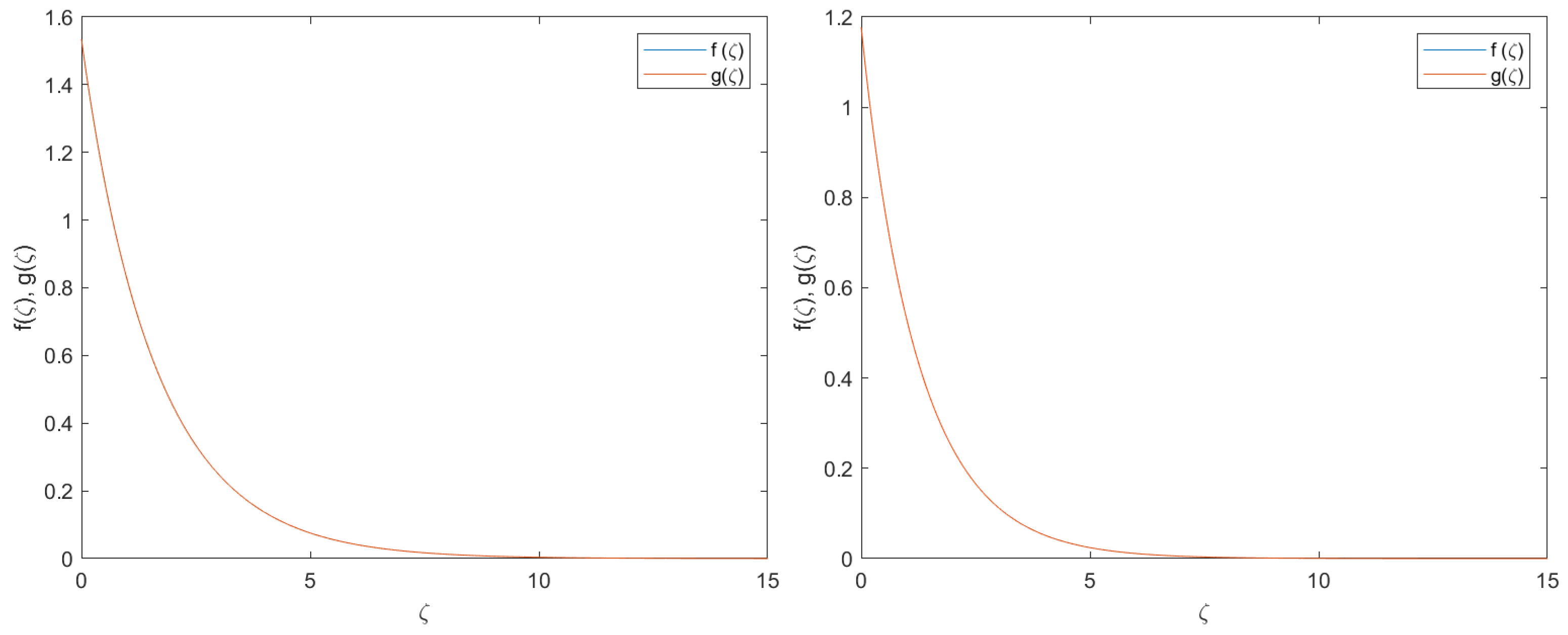
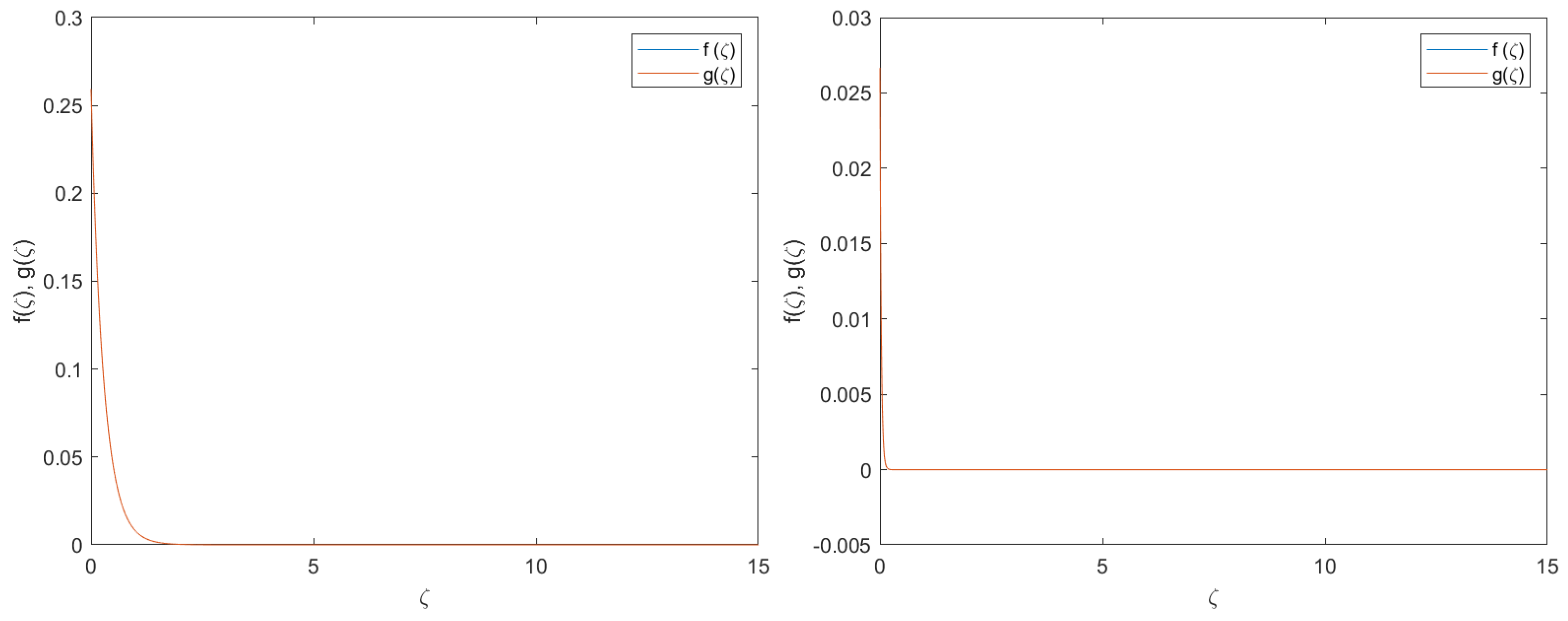
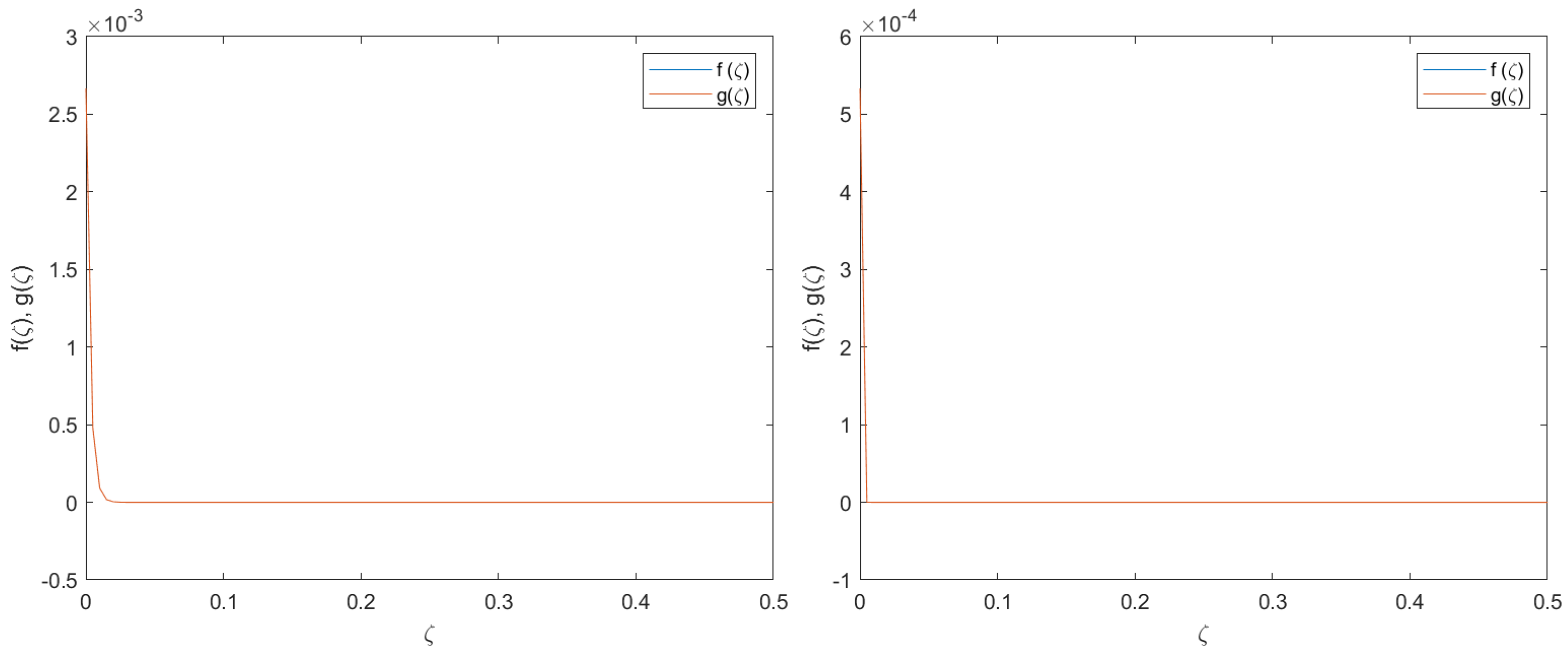
5. Numerical Assessment under the Travelling Waves Domain

This section has the objective of providing a validation of the previously introduced regularity assessments. To this end, the solutions are studied under the travelling waves domain.

The required travelling wave profiles are defined as $u\left(x,y,z,t\right) = f\left(\zeta \right),$ $v(x,y,z,t) = g\left(\zeta \right)$, $\zeta = \mathbf{x}{n}_d-ct \in R,$ where c is the travelling wave propagation speed, $n_d$ is the travelling direction; in this case, $n_d = (0,0,1)$ and $f,g:R\to \left(0,\infty \right)$ belongs to $L^{\infty }\left(R\right)$ as per the boundedness of solutions shown in (8). Then, the Equations (2) and (3) are converted to the travelling domain as follows:

$$-c{f}^{\prime }+w{f}^{\prime } = \left(\nu +\frac{1}{\beta d_1{\rho }_f}\right)f^{″}-\frac{1}{2\beta d_1^3{\rho }_f}{\left(f^{\prime }\right)}^2{f}^{″}-\frac{\sigma B_0^2}{{\rho }_f}f,$$

(9)

$$-c{g}^{\prime }+w{g}^{\prime } = \left(\nu +\frac{1}{\beta d_1{\rho }_f}\right)g^{″}-\frac{1}{2\beta d_1^3{\rho }_f}{\left(g^{\prime }\right)}^2{g}^{″}-\frac{\sigma B_0^2}{{\rho }_f}g.$$

(10)

with

$$f,g \in L^{\infty }\left(R\right),$$

and the following radially symmetrical initial functions:

$$u_0(x,y,z) = v_0(x,y,z) = e^{-(x^2+y^2+z^2)},$$

(11)

which comply with the globally bounded gradient condition, as postulated in Theorem 1. The choice of the bell-shaped initial condition is justified as follows: The problem is considered for a free geometry with no fixed boundaries, so that the bell-shaped initial conditions permit the consideration of a positive distribution that is null at $x\to \infty$, $y\to \infty$ and $z\to \infty$. Now, admit the following standard change of variable:

$$X_1 = f\left(\zeta \right),X_2 = f^{\prime }\left(\zeta \right),X_3 = g\left(\zeta \right),X_4 = g^{\prime }\left(\zeta \right)$$

so that the following system holds:

$$\begin{array}{ccc}\hfill X_1^{\prime }& = & X_2,\hfill \\ \hfill \left(\nu +\frac{1}{\beta d_1{\rho }_f}-\frac{1}{2\beta d_1^3{\rho }_f}{X}_2^2\right)X_2^{\prime }& = & -c{X}_2+\frac{\sigma B_0^2}{{\rho }_f}{X}_1\hfill \end{array}$$

(12)

$$\begin{array}{ccc}\hfill X_3^{\prime }& = & X_4,\hfill \\ \hfill \left(\nu +\frac{1}{\beta d_1{\rho }_f}-\frac{1}{2\beta d_1^3{\rho }_f}{X}_3^2\right)X_4^{\prime }& = & -c{X}_4+\frac{\sigma B_0^2}{{\rho }_f}{X}_3,\hfill \end{array}$$

(13)

where the velocity component, w, is considered as negligible compared to the velocity components $u,v$, i.e., ${\parallel w\parallel }_{\infty }\ll {\parallel u\parallel }_{L^2}$, ${\parallel w\parallel }_{\infty }\ll {\parallel v\parallel }_{L^2}$. This is equivalent to studying the profile of the flow in the $(x,y)$ plane along the z-axis (so that the velocity component, w, shall be understood as a local perturbation upon fluid motion) and along time, as per the travelling wave change of the variable.

Equations (12) and (13) are sharply solved to obtain the travelling wave profiles, $f,g$. To this end, a numerical assessment was performed according to the following main conditions:

• The numerical routine was compiled with the Matlab function, bvp4c. This function is based on a Runge–Kutta implicit approach with interpolant extensions [19]. The bvp4c collocation method required the specification of the boundary conditions, which in this case were given by the following equations:

  $$u\to 0,v\to 0,\zeta \to \infty ,$$

  (14)

  $$u = ax,v = ay,\zeta = 0,$$

  (15)

  where $a \in R$, for the numerical assessment, $a = 1$. To execute the numerical exercise, the profiles at $\zeta = 0$ were taken as a mean over a sufficiently large square so as to admit the conditions $\left|x\right|\to \infty$ and $\left|y\right|\to \infty$.
• The integration domain was considered as $\zeta \in (0,350)$, sufficiently large to admit the condition $\zeta \to \infty$, or equivalently a condition in which the collocation method in the boundaries does not impact the shape of the solution.
• The travelling wave domain was divided into 100,000 nodes, with an accumulated absolute error of ${10}^{-6}$ during the computation.
• Without loss of generality and for the sake of simplicity during the computational phase, the fluid constants in (2) and (3) were assumed to have a unity value.

Figure 1, Figure 2 and Figure 3 compile the results. It is possible to check on the regularity of solutions upon evolution along the travelling wave variable. The solutions are provided for a wide interval of travelling wave speeds, c. The increase of the speed value, c, beyond 5000 induces instabilities in the numerical computation due to the fact that the solution is within the interval error considered by the bvp4c solver.

6. Conclusions

The proposed theorem, Theorem 1, was demonstrated based on the supporting Propositions 1 and 2 and Definition 1 established in Section 3 and Section 4. Such proposed theorem permitted us to state on the $L^2$-regularity criteria the given initial data with the energetically bounded spatial gradient. The provided bounds and regularity conditions were applied to an Eyring–Powell fluid along $\Omega = R \times R \times \left[0,\infty \right)$ for $t>0$. Finally, a numerical assessment permitted the confirmation of the regularity of solutions, as proved in Theorem 1.

References

1. Ara, A.; Khan, N.A.; Khan, H.; Sultan, F. Radiation effect on boundary layer flow of an Eyring–Powell fluid over an exponentially shrinking sheet. Ain-Shams Eng. J. 2014, 5, 1337–1342. [Google Scholar] [CrossRef] [Green Version]
2. Hayat, T.; Iqbal, Z.; Qasim, M.; Obaidat, S. Steady flow of an Eyring Powell fluid over a moving surface with convective boundary conditions. Int. J. Heat Mass Transf. 2012, 55, 1817–1822. [Google Scholar] [CrossRef]
3. Hayat, T.; Awais, M.; Asghar, S. Radiative effects in a threedimensional flow of MHD Eyring-Powell fluid. J. Egypt. Math. Soc. 2013, 21, 379–384. [Google Scholar] [CrossRef] [Green Version]
4. Akbar, N.S.; Ebaid, A.; Khan, Z. Numerical analysis of magnetic field on Eyring-Powell fluid flow towards a stretching sheet. J. Magn. Magn. Mater. 2015, 382, 355–358. [Google Scholar] [CrossRef]
5. Jalil, M.; Asghar, S.; Imran, S. Self similar solutions for the flow and heat transfer of Powell-Eyring fluid over a moving surface in parallel free stream. Int. J. Heat Mass Transf. 2013, 65, 73–79. [Google Scholar] [CrossRef]
6. Khan, J.A.; Mustafa, M.; Hayat, T.; Farooq, M.A.; Alsaedi, A.; Liao, S. On model for three-dimensional flow of nanofluid: An application to solar energy. J. Mol. Liq. 2014, 194, 41–47. [Google Scholar] [CrossRef]
7. Javed, T.; Abbas, Z.; Ali, N.; Sajid, M. Flow of an Eyring–Powell nonnewtonian fluid over a stretching sheet. Chem. Eng. Commun. 2013, 200, 327–336. [Google Scholar] [CrossRef]
8. Riaz, A.; Ellahi, R.; Sait, S.M. Role of hybrid nanoparticles in thermal performance of peristaltic flow of Eyring–Powell fluid model. J. Therm. Anal. Calorim. 2021, 143, 1021–1035. [Google Scholar] [CrossRef]
9. Nadeem, S.; Malik, M.Y.; Hussain, A. Boundary layer flow of an Eyring–Powell model fluid due to a stretching cylinder with variable viscosity. Sci. Iran. 2013, 20, 313–321. [Google Scholar]
10. Bhatti, M.M.; Abbas, T.; Rashidi, M.M.; Ali, M.E.-S.; Yang, Z. Entropy generation on MHD Eyring–Powell nanofluid through a permeable stretching surface. Entropy 2016, 18, 224. [Google Scholar] [CrossRef] [Green Version]
11. Chae, D.; Wolf, J. On Liouville-type Theorems for the Steady-Navier Stokes equations in R3. J. Differ. Equ. 2016, 261, 5541–5560. [Google Scholar] [CrossRef]
12. Seregin, G. Liouville-type Theorems for the Stationary Navier-Stokes equations. Nonlineartiy 2016, 29, 2191–2195. [Google Scholar] [CrossRef] [Green Version]
13. Chamorro, D.; Jarrin, O.; Lemarie-Rieusset, P.G. Some Liouville Theorems for stationary Navier-Stokes equations in Lebesgue and Morrey Spaces. arXiv 2018, arXiv:1806.03003v1. [Google Scholar]
14. Chae, D. Liouville-type theorems for the forced Euler equations and the Navier-Stokes equations Commun. Math. Phys. 2014, 326, 37–48. [Google Scholar] [CrossRef] [Green Version]
15. Chae, D.; Yoneda, Y. On the Liouville theorem for the stationary Navier-Stokes equations in a critical space. J. Math. Anal. Appl. 2013, 405, 706–710. [Google Scholar] [CrossRef]
16. Koch, G.; Nadirashvili, N.; Seregin, G.; Šverák, V. Liouville theorems for the Navier-Stokes equations and applications. Acta Math. 2009, 203, 83–105. [Google Scholar] [CrossRef]
17. Solonnikov, V.A. Estimates of the solutions of the nonstationary Navier-Stokes system. In Boundary Value Problems of Mathematical Physics and Related Questions in the Theory of Functions, 7th ed.; Zapiski Nauchnykh Seminarov LOMI; Nauka: Sankt Petersburg, Russia, 1973; Volume 38, pp. 153–231. [Google Scholar]
18. Azzam, J.; Bedrossian, J. Bounded mean oscillation and the uniqueness of active scalar equations. Trans. Am. Math. Soc. 2015, 367, 30953118. [Google Scholar] [CrossRef] [Green Version]
19. Enright, H.; Muir, P.H. A Runge-Kutta Type Boundary Value ODE Solver with Defect Control; Tehnical Report 267/93; Department of Computer Sciences, University of Toronto: Toronto, ON, Canada, 1993. [Google Scholar]
Figure 1. c   =   0.1 (left), c   =   1 (right). Representation of the solutions in the travelling wave domain evolving along the ζ domain. Note that both solutions, f , g , are superimposed. It is possible to check the regularity of solutions.
Mathematics 10 00741 g001
Figure 2. c   =   10 (left), c   =   100 (right). Representation of the solutions in the travelling wave domain evolving along the ζ domain. Note that both solutions, f , g , are superimposed. Once again, it is possible to check the regularity of solutions.
Mathematics 10 00741 g002
Figure 3. c   =   1000 (left), c   =   5000 (right). Representation of the solutions in the travelling wave domain evolving along the ζ domain. Note that both solutions, f , g , are superimposed. It is possible to check the regularity of solutions.
Mathematics 10 00741 g003
Publisher’s Note: MDPI stays neutral with regard to jurisdictional claims in published maps and institutional affiliations.