Optimal Experimental Design for Parametric Identification of the Electrical Behaviour of Bioelectrodes and Biological Tissues

Abstract

The electrical behaviour of a system, such as an electrode–tissue interface (ETI) or a biological tissue, can be used for its characterization. One way of accomplishing this goal consists of measuring the electrical impedance, that is, the opposition that a system exhibits to an alternating current flow as a function of frequency. Subsequently, experimental impedance data are fitted to an electrical equivalent circuit (EEC model) whose parameters can be correlated with the electrode processes occurring in the ETI or with the physiological state of a tissue. The EEC used in this paper is a reasonable approach for simple bio-electrodes or cell membranes, assuming ideal capacitances. We use the theory of optimal experimental design to identify the frequencies in which the impedance is measured, as well as the number of measurement repetitions, in such a way that the EEC parameters can be optimally estimated. Specifically, we calculate approximate and exact D-optimal designs by optimizing the determinant of the information matrix by adapting two of the most algorithms that are routinely used nowadays (REX random exchange algorithm and KL exchange algorithm). The D-efficiency of the optimal designs provided by the algorithms was compared with the design commonly used by experimenters and it is shown that the precision of the parameter estimates can be increased.

1. Introduction

The electrical behaviour of cells, biological tissues, or electrode-tissue interfaces can be used for their characterization [1,2,3,4]. One way to do this is by measuring the electrical impedance, that is, the opposition that the system under study exhibits to an alternating current flow as a function of frequency. Subsequently, experimental impedance data are fitted to an electrical equivalent circuit (EEC), which is a mathematical model that approximates the electrical behaviour of the system under study. Thus, the EEC parameters give information about the physiological state of a tissue or about the electrode processes occurring in the electrode-tissue interface (ETI). For instance, it is useful to know the electrical/electrochemical behaviour of the ETI plays a significant role in the biopotential measurements or also in the propagation of an applied stimuli. It should be mentioned that the experimental impedance data are analysed by using an impedance function. This impedance function can be proposed from a plausible physical theory (that predicts the impedance) or from an EEC, that aids in the visualization of the physical processes occurring in the system under study [1].

In this paper, we work with linear time-invariant (LTI) circuits, that is, LTI systems that fulfil the properties of linearity and invariance in time, meaning that the superposition and proportionality principles are hold. From the study of the circuit theory, a LTI circuit in which the input $i\left(t\right)$ is an electrical current (amperes), the output $v\left(t\right)$ is a voltage (volts), and t is the time (seconds) can be described by an ordinary, linear differential equation (ODE) with constant coefficients $a_i,b_j\in \mathbb{R}$ and order n for $n,m\in \mathbb{N}$ as [5]:

$$\frac{d^{n}v\left(t\right)}{d{t}^n}+a_{n-1}\frac{d^{n-1}v\left(t\right)}{d{t}^{n-1}}+\cdots +a_{0}v\left(t\right)=b_m\frac{d^{m}i\left(t\right)}{d{t}^m}+b_{m-1}\frac{d^{m-1}i\left(t\right)}{d{t}^{m-1}}+\cdots +b_{0}i\left(t\right)$$

(1)

Without loss of generality, we have assumed that $a_n=1$.

Let us now consider the input $i\left(t\right)=e^{st}$, where s is a time-independent parameter. It can be shown that the output (refer to Equation (1)) can be written as $v\left(t\right)=Z\left(s\right)e^{st}$, where $Z\left(s\right)$ is an impedance function (in units of ohms, $\mathsf{\Omega }$), which relates the voltage to the current:

$$Z\left(s\right)=\frac{b_m{s}^m+b_{m-1}{s}^{m-1}+\cdots +b_0}{s^n+a_{n-1}{s}^{n-1}+\cdots +a_0}$$

(2)

The input given by $e^{st}$ is extremely versatile. It allows us to obtain the forced response to a constant input ($s=0$) or to a sinusoidal input ($s=j\omega$, where j is the imaginary unit and $\omega$ is the angular frequency in rad/s with $\omega =2\pi f$, where f is frequency in Hz). This latter response is known as frequency response of systems, that is, the response of a system to input sinusoids of different frequencies. Moreover, $e^{st}$ constitutes a basis function involving the Fourier series and the Fourier and Laplace transforms [5].

Note in particular that the parameter s in (2) can be interpreted as the variable that appears in the Laplace transform or as the differential operator ($\frac{d}{dt}$, typically denoted by p) [6]. When $s=j\omega$, the circuit is operating at sinusoidal steady-state. Specifically, by considering the Laplace transform of Equation (1), assuming zero initial conditions, we can write $V\left(s\right)=Z\left(s\right)I\left(s\right)$, where $I\left(s\right)$ and $V\left(s\right)$ are the Laplace transforms of the input $i\left(t\right)$ and the output $v\left(t\right)$, respectively. Interestingly, the unit-impulse ($i\left(t\right)=\delta \left(t\right)$, $I\left(s\right)=1$, where $\delta \left(t\right)$ is Dirac delta function) response is $V\left(s\right)=Z\left(s\right)$, that is, the Laplace transfom of the voltage output equal the impedance $Z\left(s\right)$.

Electrical impedance has been usually defined in the context of a single sinusoidal signal and phasor analysis [6]. The impedance $Z\left(j\omega \right)$ at the frequency $\omega$, is a complex number whose magnitude and phase are $\left|Z\right(j\omega \left)\right|$ and $arg\left[Z\right(j\omega \left)\right]$, respectively. Equivalently, $Z\left(j\omega \right)$ can also be expressed in terms of its real and imaginary components, that is, the resistance $R\left(\omega \right)$ and the reactance $X\left(\omega \right)$, respectively.

$$Z\left(j\omega \right)={\left|Z\left(j\omega \right)\right|}_{arg\left[Z\right(j\omega \left)\right]}=R\left(\omega \right)+jX\left(\omega \right)$$

(3)

Note that for physical frequencies ($s=j\omega$), the impedance in Equation (2) can be written according to Equation (3). Hereinafter, the impedance $Z\left(j\omega \right)$ is also denoted by $Z\left(\omega \right)$.

Regarding the sinusoidal signal, it should be mentioned that the square of the rms (root mean square) value of a sinusoidal signal is the average power associated with it, that is, the average power is concentrated at frequency $\omega$. Importantly, the average power associated with a periodic signal is the sum of the squared rms values (sum of the average powers) of all its components (Parseval’s theorem for periodic signals). Therefore, the power spectral density (which, when integrated over the whole spectrum frequency, gives the total average power) for a periodic signal (power signal) consists of a series of impulses [7].

In this paper, we focus on finding the input frequencies to the circuit which maximises the amount of information obtained from an experiment, given that the true system is a priori known. Optimal input designs concern finding the input signal, which assures that the estimates become as good as possible. The use of optimal input signals will increase the precision of the parameter estimators [8]. This problem, called optimal input design, arises from the works of Mehra [9,10]. The theory of optimal design of experiments for the construction of optimal input signals in control theory, involving the frequency domain, can be found in [11,12,13,14,15,16,17,18]. However, its use for electrical impedance models has been scarcely reported in the scientific literature. Considerations of optimal multisine input signals are analysed in [19,20,21]. Specifically, a D-optimal multisine excitation for broadband impedance spectroscopy measurements is proposed in [20]. These optimal designs are based on simple first-order LTI circuits, that is, they are described by an ODE of order 1. The objective of this work is to design the D-optimal frequencies in which to carry out the electrical impedance measurements to achieve the best statistical estimates. Specifically, we calculate approximate and exact optimal designs by optimizing the determinant of the information matrix by adapting the REX random exchange algorithm and KL exchange algorithm. To the best of the authors’ knowledge, there is no previous report of modifying those algorithms to calculate D-optimal designs in the frequency domain. In Section 2, we provide an introduction to the D-optimal input design applied to the study of a simple impedance model, which approaches the electrical behaviour of basic bio-electrodes or cell membranes. The definition of the Fisher Information Matrix (FIM) and the spectral density function are presented. Section 3 is devoted to the D-optimization criterion, the directional derivative, the equivalence theorem and the two algorithms adapted. Finally, in Section 4, we include a real application. The results obtained from an experimental test carried out with the two algorithms adapted to compare the efficiency of the design commonly used by experimenters with the D-optimal designs obtained from the algorithms are also discussed in this section.

2. Optimal Experimental Design for the Identification of LTI Systems

In general, the procedure for the identification of a system can be divided into three steps. The first one will be the experimental design, that is, planning and selecting the input signals to be introduced into the model. The set where to take the observations is known as the design space and is denoted by $\chi$. From now on we will assume that it is a compact set. Once the input signals have been selected within the design space, the second step will be to collect data. The third step will be to estimate the parameters of the model.

2.1. Design of Experiments Background

Let $\chi$ be the compact design space and $y\left(t\right)$ the response variable, assumed as a random variable of a parametric distribution with a vector of parameters $\theta$. We assume that the observations $y\left(t\right)$ verify the following model:

$$y\left(t\right)=\eta (t,\theta )+\epsilon \left(t\right)$$

(4)

The model exhibits a random error $\epsilon$ and the function $\eta$ is called the response surface and it is a partially known function, that is, it is within a parametric set of functions where the parameters ${\theta }^T=({\theta }_1,\dots ,{\theta }_k)\in {\mathbb{R}}^k$ are unknown and their specification determines $\eta$ totally. The response variable depends on the variable t, which we will call the independent or design variable, which can be freely chosen by the experimenter.

We will say that an exact design, ${\xi }_N$ is a collection of N different support points, $t_1,t_2,\dots ,t_N$, where there could be repetitions. An approximate design, $\xi$, is a collection of M different support points, $t_1,t_2,\dots ,t_M$, and weights, $\xi \left(t_1\right),\xi \left(t_2\right),\dots ,\xi \left(t_M\right)$, that defines a discrete probability at $\chi$. If the design $\xi$ has weight $\xi \left(t_i\right)$ at $t_i$, $i=1,\dots ,M$ and the total number of observations made is N, approximately $N\xi \left(t_i\right)$ observations will be taken at $t_i$, $i=1,\dots ,M$. By choosing a sufficiently large N, it is possible to approximate a design with these characteristics to an exact design. The approximations will be better the larger the N [22].

One of the most important tools in the optimal experimental design is the FIM induced by $\xi$. The variance-covariance matrix $Var\left[\widehat{\theta }\right]$ of the maximum likelihood estimator $\widehat{\theta }$ can be asymptotically approximated by the inverse of the FIM, $M^{-1}\left(\xi \right)$, and under certain regularity conditions it reaches the lower limit of Cramer-Rao [23]. Once the estimator has been specified, we can consider the optimal design problem, as the selection of predictors that somehow lead to the minimization of the variance-covariance matrix $Var\left[\widehat{\theta }\right]\approx M^{-1}\left(\xi \right)$, or equivalently to the maximization of $M\left(\xi \right)$. Therefore, the objective of the optimal design of experiments will be to find the best of the designs that maximizes $M\left(\xi \right)$ or minimizes $M^{-1}\left(\xi \right)$ in some sense.

Optimal design theory was initially developed for linear models. However, in practice it is common to find experiments where the response is explained from non-linear models in the parameters to be estimated, as this case study. The most common method for analysing data from a non-linear model is based on the use of the linear Taylor series approximation of the response surface.

$$\eta (t,\theta )\approx \eta (t,{\theta }^{\left(0\right)})+{\left[{\nabla }_{\theta }\eta (x,\theta ){|}_{{\theta }^{\left(0\right)}}\right]}^T(\theta -{\theta }^{\left(0\right)})$$

(5)

where ${\nabla }_{\theta }$ denotes the gradient with respect $\theta$ and being ${\theta }^{\left(0\right)}$ a prior value of $\theta$, for example an estimate calculated on the basis of an initial experiment or suitable values found in the literature. Thus, the FIM will depend on the values of the unknown parameters and, consequently, the optimal designs will also depend on these values,

$$M(\xi ,\theta )={\int }_{\xi }{\nabla }_{\theta }\eta (t,\theta ){\nabla }_{\theta }^T\eta (t,\theta )\xi \left(dt\right)$$

(6)

2.2. Electrical Circuit Model

Let us consider the EEC of Figure 1A. It comprises a resistance $R_1$ in series with the parallel combination of a capacitor C and a resistance $R_2$. Currents and voltages have been labelled in each element. $i\left(t\right)$ and $v\left(t\right)$ are the current input and the voltage output, respectively. $i_C\left(t\right)$ and $i_{R_2}\left(t\right)$ are the currents flowing through the capacitor C and the resistance $R_2$, respectively. $v_C\left(t\right)$ is the voltage across C (the same than that of $R_2$).

The ODE of the EEC shown in Figure 1A is written as (refer to Appendix A)

$$\frac{dv\left(t\right)}{dt}+a_{0}v\left(t\right)=b_1\frac{di\left(t\right)}{dt}+b_{0}i\left(t\right),t\in [0,T]$$

(7)

Let us define ${\theta }^T=(b_1,b_0,a_0)$ for $b_1,b_0,a_0\in \mathbb{R}$ and $k=3$ the unknown vector parameters with

$$\left\{\begin{array}{cc}\hfill b_1=& R_1\hfill \\ \hfill b_0=& \frac{R_1+R_2}{R_{2}C}\hfill \\ \hfill a_0=& \frac{1}{R_{2}C}\hfill \end{array}\right.$$

(8)

As we saw in Section 1, the impedance from Equation (7) is obtained as

$$Z\left(s\right)=\frac{b_{1}s+b_0}{s+a_0}$$

(9)

For physical frequencies $s=j\omega$, Equation (9) is written as

$$Z\left(\omega \right)=\frac{b_{1}j\omega +b_0}{j\omega +a_0}$$

(10)

where $\omega \in (0,\infty )$.

Figure 1B shows the Nyquist plot ($-X\left(\omega \right)$ vs. $R\left(\omega \right)$ in the complex plane). Equation (10) sketches a semicircle, which intersects the real axis at $R_1$ and $R_1+R_2$, at the frequencies $\omega =\infty$ and $\omega =0$, respectively ($\omega$ is positive and increases counterclockwise). The maximum of $-X\left(\omega \right)$ vs. $R\left(\omega \right)$ is reached at ${\omega }_{\max }=\frac{1}{R_{2}C}$.

Now, let the parameter s (refer to Equation (9)) be considered the differential operator, that is, $p=d/dt$ (see above). The unknown parameters $\theta$ must be estimated from measures of the form:

$$v\left(t\right)=Z\left(p\right)i\left(t\right)+\epsilon \left(t\right)$$

(11)

where $Z\left(p\right)$ is a new differential operator [6] and $\epsilon \left(t\right)$ is a random error $N(0,{\sigma }^2)$ that includes both the errors of the tests and the specification of the model. The Fourier transform of Equation (11) is given by

$$V\left(\omega \right)=Z\left(\omega \right)I\left(\omega \right)+E\left(\omega \right)$$

(12)

where $V\left(\omega \right)=\mathcal{F}\left[v\right]\left(\omega \right)\in \mathbb{C}$, $I\left(\omega \right)=\mathcal{F}\left[i\right]\left(\omega \right)\in \mathbb{C}$ and $E\left(\omega \right)=\mathcal{F}\left[\epsilon \right]\left(\omega \right)\in \mathbb{C}$, with $\mathcal{F}$ the Fourier transform.

It should be mentioned that the impedance of (9) can also be obtained by considering the impedance of each of $R_1$, $R_2$ and C, that is, $R_1$, $R_2$ and $\frac{1}{sC}$, respectively, resulting in $Z\left(s\right)=R_1+(R_2\Vert \frac{1}{sC})$, ‖ denotes parallel, which gives Equation (9).

2.3. The FIM for the Electrical Circuit Model

In this section, we will consider that the input signal $i\left(t\right)$ is a time stationary process and we will go from the time domain to the frequency domain in order to apply the optimal design theory for this type of LTI SISO (single-input, single-output) systems. In this domain, the properties for the approximation of the information matrices used in the theory of the optimal design of experiments, given by Kiefer-Wolfowitz [24], Karlin-Studden [25] and Fedorov [26], are preserved. According to Mehra [9], if a SISO system is LTI, the number of data points N is large and $i\left(t\right)$ is a stationary process, the optimal inputs can be calculated much more efficiently using frequency domain techniques.

Let Equation (10) be the impedance model to be estimated, where $\theta$ is the vector of parameters of the impedance model defined in (8). Then,

$${\nabla }_{\theta }Z\left(\omega \right)=\left(\begin{array}{c}\frac{j\omega }{j\omega +a_0}\\ \frac{1}{j\omega +a_0}\\ -\frac{j(b_1\omega -b_{0}j)}{{(j\omega +a_0)}^2}\end{array}\right)$$

(13)

By Parseval’s Theorem, we find that, for a continuous time model (10), the FIM in the frequency domain is given by (refer to Appendix B)

$$M\left(\mathsf{\Phi }\right)=\frac{1}{2\pi }{\int }_{-\infty }^{+\infty }\tilde{M}(\omega ,\theta )\mathsf{\Phi }\left(\omega \right)d\omega$$

(14)

where $\mathsf{\Phi }$ is the power spectral density of $i\left(t\right)$ and $\tilde{M}(\omega ,\theta )$ is the single-frequency FIM, which defines the information associated with the model (10) with respect to $\theta$, defined as

$$\tilde{M}(\omega ,\theta )=\Re \left\{{\nabla }_{\theta }Z\left(\omega \right)·{\nabla }_{\theta }Z{\left(\omega \right)}^H\right\}$$

(15)

where the superscript H denotes the conjugate transpose operator and $\Re \left\{z\right\}$ is the real part of the number $z\in \mathbb{C}$. From the model (10), the single-frequency FIM as defined in (15) is

$$\tilde{M}(\omega ,\theta )=\left(\begin{array}{ccc}\frac{{\omega }^2}{a_0^2+{\omega }^2}& 0& \frac{{\omega }^2(b_0-b_1{a}_0)}{{(a_0^2+{\omega }^2)}^2}\\ 0& \frac{1}{a_0^2+{\omega }^2}& -\frac{b_1{\omega }^2+b_0{a}_0}{{(a_0^2+{\omega }^2)}^2}\\ \frac{{\omega }^2(b_0-b_1{a}_0)}{{(a_0^2+{\omega }^2)}^2}& -\frac{b_1{\omega }^2+b_0{a}_0}{{(a_0^2+{\omega }^2)}^2}& \frac{b_1^2{\omega }^2+b_0^2}{{(a_0^2+{\omega }^2)}^2}\end{array}\right)$$

(16)

Note that in the frequency domain, the role of the probability measure is played by the power spectral density function $\mathsf{\Phi }$. Therefore, $\mathsf{\Phi }$ is the design measure (or design), $\xi$, that we call in the context of design of experiments.

We define by $\Xi$ the set of non-decreasing, continuous design measures of bounded variation, corresponding to input power spectral density functions, that is,

$$\Xi =\left\{\mathsf{\Phi }:{\int }_{{\omega }_I}^{{\omega }_E}\mathsf{\Phi }\left(\omega \right)d\omega =1\right\}$$

(17)

The design can be limited to a finite range $[{\omega }_I,{\omega }_E]$, where ${\omega }_I$ and ${\omega }_E$ are the lowest and highest angular frequencies, respectively, at which impedance has been measured. This frequency range will be the design space $\chi$.

3. Construction of D-Optimal Input Signals

Among a set of designs, it is not easy to decide which is “the best” of them. Therefore, we need to choose a criterion, a scalar measure of the FIM, $\mathsf{\Psi }:\mathcal{M}(\Xi )⟶\mathbb{R}\cup \{\infty \}$, called optimality criterion, that helps us to find the best design. The choice will depend on the interests sought by conducting the experiment. A design that minimizes $\mathsf{\Psi }$ over all the designs on $\chi$ is called an optimum design, that is

$${\mathsf{\Phi }}^{*}=arg\underset{\mathsf{\Phi }\in \Xi }{min}\mathsf{\Psi }\left[M\left(\mathsf{\Phi }\right)\right]$$

(18)

The most popular criterion is D-optimality. This criterion consists of minimizing the volume of the confidence ellipsoid of estimators of the parameters of the model, i.e., it maximizes the determinant of the FIM. For a given ${\theta }^{\left(0\right)}$, D-optimality is defined by the criterion function:

$${\mathsf{\Psi }}_D\left[M\left(\mathsf{\Phi }\right)\right]={[detM\left(\mathsf{\Phi }\right)]}^{-\frac{1}{k}}$$

(19)

When an optimal design is sought among all approximate designs on the design space and the design criterion is convex, it can be checked the optimality of a particular design using the celebrated General Equivalence Theorem (GET) [24]. If the criterion function, $\mathsf{\Psi }$, is differentiable the GET has a friendly version. Thus, a design ${\mathsf{\Phi }}_D^{*}$ is ${\mathsf{\Psi }}_D$-optimum if and only if $\forall \omega \in \chi$, the dispersion function

$$d(\omega ,{\mathsf{\Phi }}_D^{*})={\nabla }_{\theta }Z{\left(\omega \right)}^H{M}^{-1}\left({\mathsf{\Phi }}_D^{*}\right){\nabla }_{\theta }Z\left(\omega \right)=Tr\left[M^{-1}\left({\mathsf{\Phi }}_D^{*}\right)\tilde{M}(\omega ,\theta )\right]$$

(20)

achieves its maximum values at the support points. In particular, for the D-optimum criterion this condition proves the optimality of ${\mathsf{\Phi }}_D^{*}$ if and only if

$$d(\omega ,{\mathsf{\Phi }}_D^{*})\le k,\forall \omega \in \chi$$

(21)

being k the number of the parameters of the model.

The GET allows us to check the optimality of a design, but it does not tell us how to find it. However, this theorem is useful for building efficient algorithms that allow computing optimal designs.

Another fundamental tool commonly used by the algorithmic techniques is the efficiency of a design. This value is interpretated as the goodness of a design and is defined as $Ef{f}_{\mathsf{\Psi }}\left(\mathsf{\Phi }\right)=\mathsf{\Psi }\left[M\left(\mathsf{\Phi }\right)\right]/\mathsf{\Psi }\left[M\left({\mathsf{\Phi }}^{*}\right)\right]$, being ${\mathsf{\Phi }}^{*}$ the $\mathsf{\Psi }$-optimal design. Thus the D-efficiency of a design ${\mathsf{\Phi }}_D$ is computed as:

$$Ef{f}_D\left({\mathsf{\Phi }}_D\right)={\left[\frac{detM\left({\mathsf{\Phi }}_D\right)}{detM\left({\mathsf{\Phi }}_D^{*}\right)}\right]}^{-\frac{1}{k}}$$

(22)

If the criteron function has a homogeneity property, as in this case, there is a practical statistical interpretation. Thus, if a design has 50 % efficiency, then half of the observations with the optimal design will produce the same results with respect to the criterion function. Although this quantity cannot be calculated when the optimal design is unknown, it is possible to obtain lower limits of efficiency to make a stopping rule. An important bound for the D-optimization criterion is the one proposed by Atwood [27]

$$Ef{f}_D\left({\mathsf{\Phi }}_D\right)\ge \frac{k}{{max}_{\omega \in \chi }d(\omega ,{\mathsf{\Phi }}_D)}$$

(23)

Modified Algorithms

The search for analytical solutions for the problem of construction of optimal designs turns out to be a difficult task and, in most of the real problems, it is not possible to calculate analytically the designs under a certain criterion. There is a rich literature on numerical computational algorithms proposed to obtain optimal designs under different scenarios. In exact design problems, we do not have a convex optimization problem in general and, so, finding optimal design is not an easy task because it is a discrete optimization problem and there is no general analytical tool for confirming whether an exact design is optimal or not. There are several numerical algorithms for finding optimal exact designs based on exchange methods. In this paper, we proposed the Atkinson and Donev KL exchange algorithm [28] to calculate exact D-optimal designs. The procedure starts with a non-singular random design. Then, two sets of points are constructed from the dispersion function. One with K “least promising” support points of the current design, for which exchanges are attempted. The other one with L “most promising” candidate design points. Finally, it adds and deletes observation points that lead to the greatest increase in the determinant of the FIM, under the standard constraint of the required number of points and the maximum execution time of the algorithm. Each exchange of improvement is executed immediately. Because this is only a heuristic, it cannot be guaranteed to reach the global optimum, so it is convenient to run the algorithm several times. The end result is the best design found in all runs.

For optimal approximate design problems, there are many analytic methods to construct them. Due to the performance and the flexibility to be applied in a broad range of problem structures and sizes, the randomized exchange algorithm (REX) [29] has been considered in this work. The REX method, which is a simple batch-randomized exchange algorithm, can be viewed as an efficient extension or combination of both the vertex exchange method for D-optimality of Böhning [30] and the KL exchange algorithm. The procedure begins with a random design of non-singular points and their respective proportions. Then, a batch consisting of a pair of points is repeatedly selected: a random support point of the current design, ${\omega }_k$, and a random design point, ${\omega }_l$, where optimal ratio exchanges between these pairs are made. The batch selection depends on the dispersion function. The key to making the optimal random exchanges of proportions between the selected batch is the optimal step length value ${\alpha }_{k,l}^{*}\left({\mathsf{\Phi }}_D\right)$ (see Appendix A in [29]), which gives the value to be added or subtracted from the proportions of each observation point. Finally, it adds and deletes observation points that lead to the largest increase in the efficiency bound. This algorithm has a standard threshold constraint on the minimum design efficiency to stop the computation. The limit used as the stopping rule is the Atwood limit (23).

These algorithms were adapted to involve complex variables. The matrix of Equation (13) is given as input for both algorithms. We develop a complex type null matrix and then it is completed by creating a loop, where each row of the complex null matrix is replaced by the components of (13). Each row corresponds to a value of $\omega$ within $\chi$ previously defined. Next, we adapt the definition of the single frequency FIM (see Equation (15)) and the dispersion function (20). Modified codes to adapt the algorithms to this case study can be found in Appendix C.

The general procedure followed by these algorithms can be summarized as:

• An initial design is chosen. In principle, it can be any arbitrary design, ${\mathsf{\Phi }}_D^{\left(0\right)}$, such that the criterion function for this design verifies ${[detM\left({\mathsf{\Phi }}_D^{\left(0\right)}\right)]}^{-\frac{1}{k}}\ne 0$.
• A succession of designs ${\mathsf{\Phi }}_D^{\left(1\right)},{\mathsf{\Phi }}_D^{\left(2\right)},\dots$ is obtained computationally in an iterative way, where ${\mathsf{\Phi }}_D^{(q+1)}$ is calculated by slightly disturbing the previous design ${\mathsf{\Phi }}_D^{\left(q\right)}$ and requiring that ${[detM\left({\mathsf{\Phi }}_D^{(q+1)}\right)]}^{-\frac{1}{k}}\ne 0$.
• The process of generating the previous designs will end in the qth step after verifying that the design ${\mathsf{\Phi }}_D^{\left(q\right)}$ obtained is close enough to the optimum according to a stopping rule.

4. Real Applications

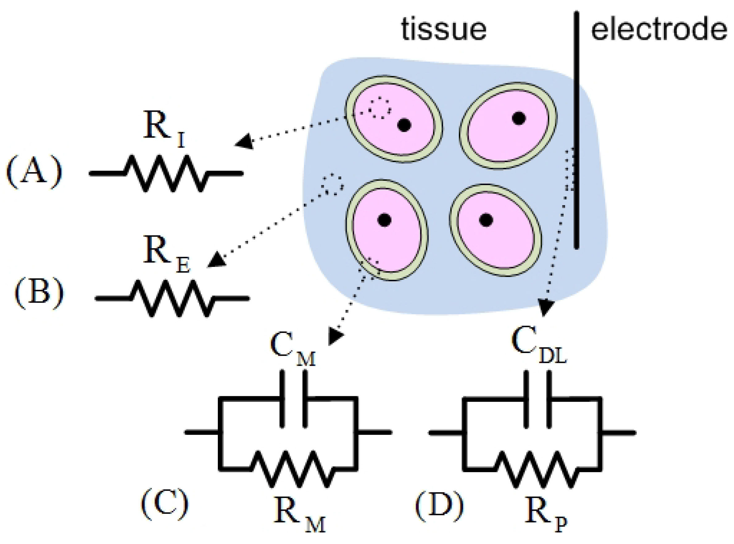
As mentioned earlier, biological tissues, cells, and ETIs can be characterized from their electrical behaviour. Figure 2 shows a portion of tissue (group of similar cells) with an implanted electrode. In general, the passive electrical behaviour of the tissue and the ETI involve electrical capacitance (capacity to store charges) and resistance (ability to oppose dc-current flow). Figure 2 also shows several basic EECs [1,2,3,4]. Intra- (pink colour) and extracellular (blue colour) media are resistive parts (electrolyte solutions), and thus are modelled by the resistances $R_I$ (Figure 2A) and $R_E$ (Figure 2B), respectively. The passive electrical behaviour of a cell membrane (green colour) is described by a parallel combination of a cell membrane capacitance $C_M$ and the membrane resistance $R_M$ (see Figure 2C). 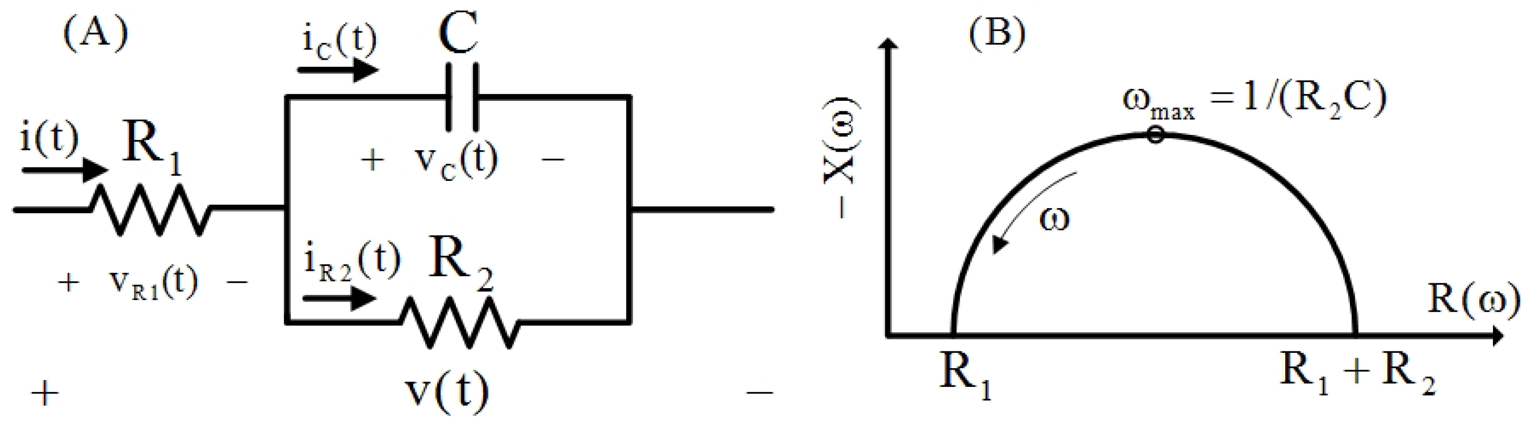A basic model of ETI is shown in the EEC of Figure 2D, that is, a double layer capacitance $C_{DL}$ in parallel with the polarization resistance $R_P$[1,3]. The EEC shown in Figure 1A involves those of Figure 2C,D with an additional resistance $R_1$. Moreover, the impedance of the EEC of Figure 1A is equivalent to that proposed by Cole when the biological tissue involves an ideal capacitance [2,4].

It should be mentioned that the optimal design of experiments is of great interest for two main reasons: to obtain an optimal characterization of the process and to minimize the measurement acquisition time.

4.1. Methods

The modified algorithms were applied to the circuit shown in Figure 1A. Let $R_1=100\Omega$, $R_2={10}^6\Omega$ and $C={10}^{-6}\mathrm{F}$ the nominal values of the parameters and $\chi =[2\pi {10}^{-1},2\pi 10]$ rad/s. For numerical study, we consider the frequency design space to be a set of grid points spread equidistantly by $0.01$.

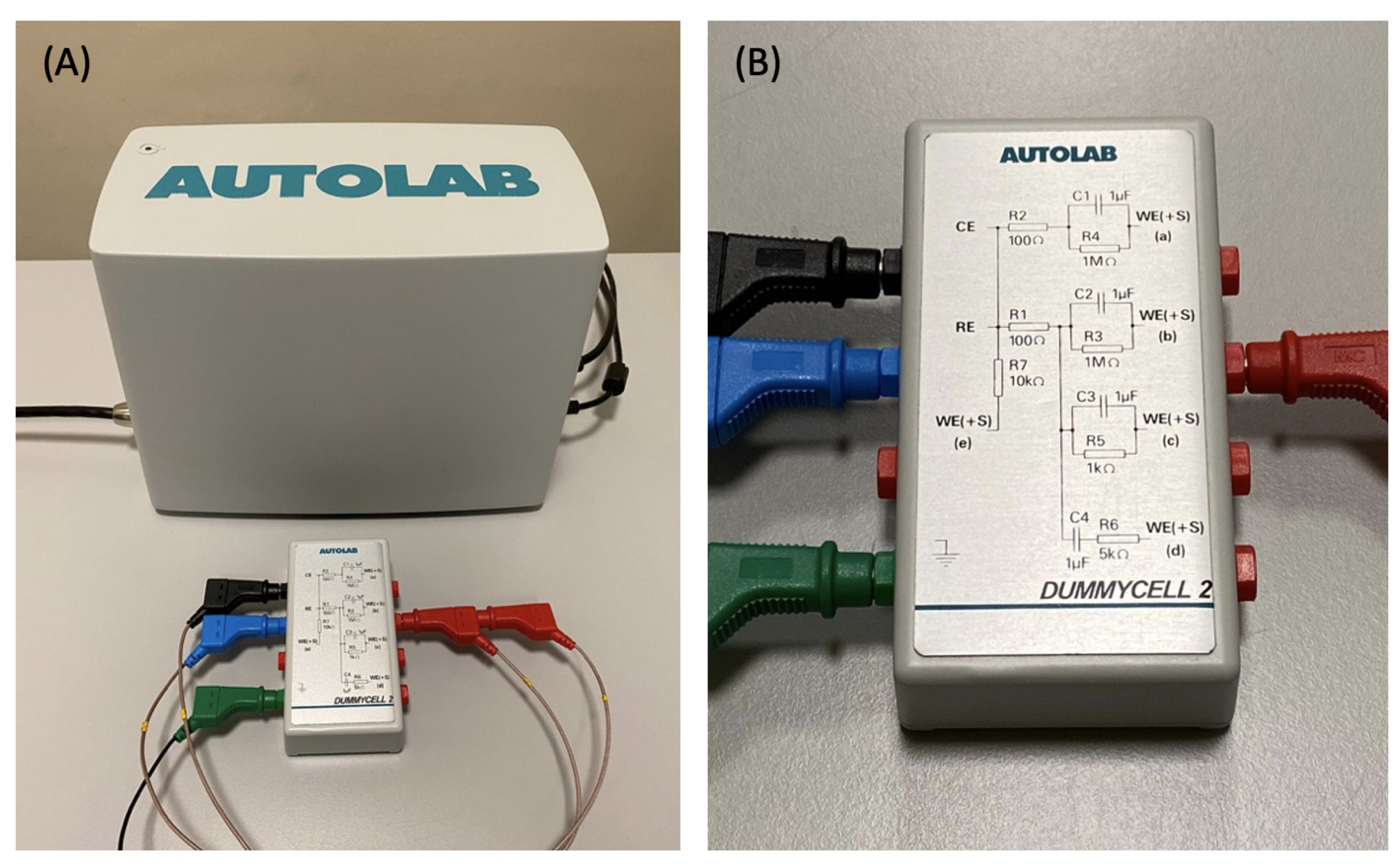
We have used the RStudio 1.3.1093 program to obtain the optimal designs. The Autolab PGSTAT204 potentiostat/galvanostat (Figure 3A), equipped with the FRA32M module, was used to perform the impedance measurements. The equipment, controlled by a computer and NOVA electrochemistry software, is connected to a dummy cell containing the circuit described above to perform the test (Figure 3B). We used sinusoidal current signals of ${10}^{-6}$ A peak amplitude.

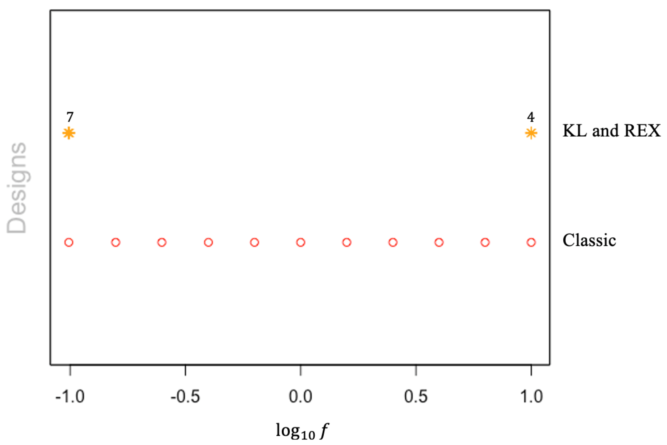
The objective of this experimental test was to compare the efficiency of the classical design commonly used by experimenters with the D-optimal designs obtained in the adapted KL and REX algorithms. The classic design is based on measuring impedance at certain frequencies equally spaced on a logarithmic scale. In particular

$${\mathsf{\Phi }}^{\mathrm{classic}}=\{2\pi {10}^{-1},2\pi {10}^{-0.8},2\pi {10}^{-0.6},\dots ,2\pi {10}^{0.8},2\pi 10\}$$

(24)

where $N=11$. For comparison purposes, the adapted KL algorithm was executed considering the same number of support points as the classic design ($N=11$). In the case of the REX algorithm, from a theoretical point of view, it is not necessary to set N. The algorithm provides points and the proportions to be measured at those points. In order to be able to compare the design obtained, the proportion was rounded to the nearest integer, that is, if the design puts weight $p_i$ on ${\omega }_i$, $i=1,\dots ,M$ and the total number of observations we want is $N=11$, then approximately $N·p_i$ observations will be taken at ${\omega }_i$, $i=1,\dots ,M$.

4.2. Results and Discussion

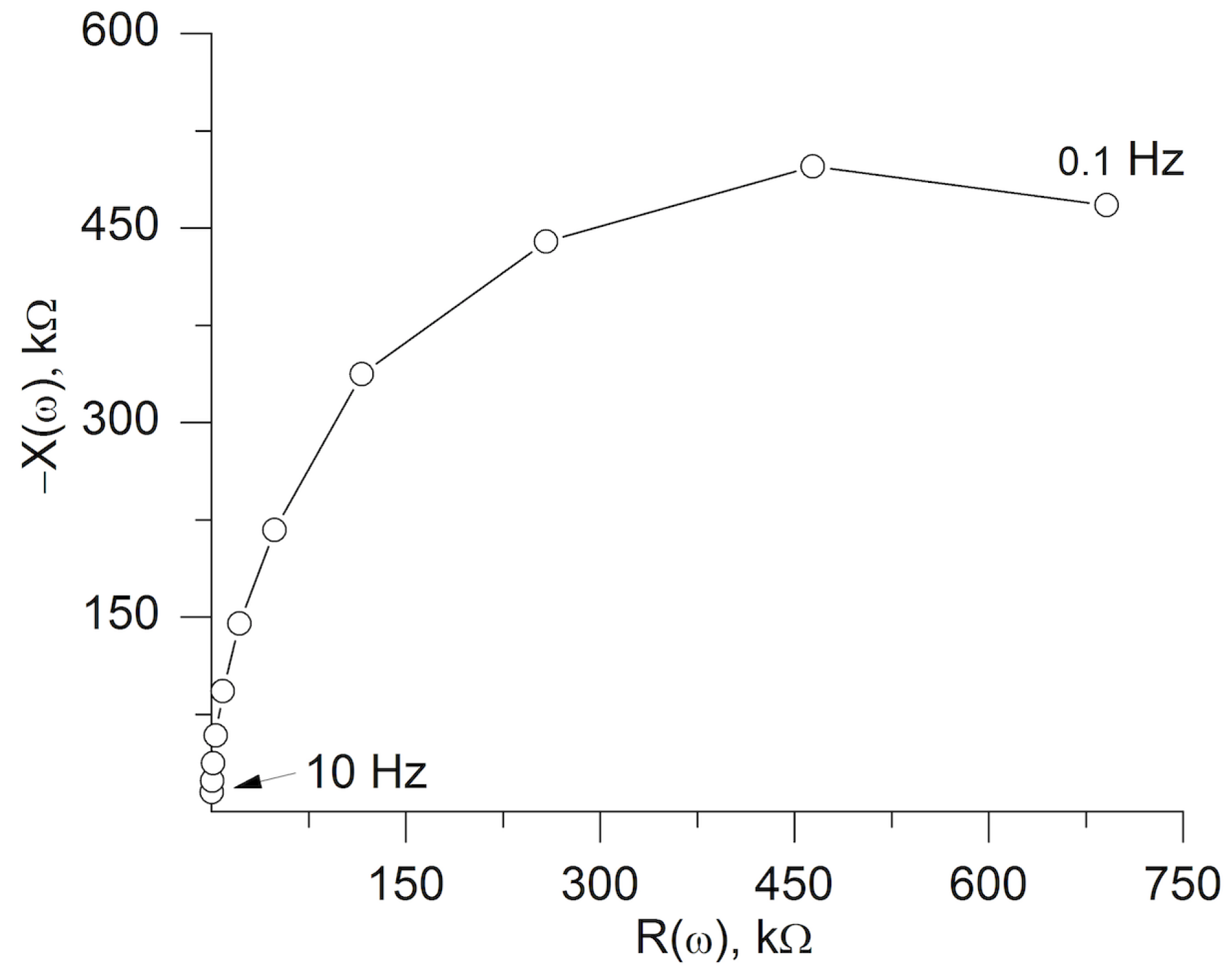
Figure 4 shows the Nyquist plot for the EEC of Figure 3B. Experimental impedance data obtained for the frequencies of (24) draw a semicircle like that of Figure 1B. Subsequently, experimental data have been fitted to the EEC of Figure 1A and the values of its parameters are given in

Table 1. EEC parameters values estimated using the different optimal designs.

Design	Iteration	N	${\mathbf{R}}_1,\mathsf{\Omega }$	${\mathbf{R}}_2,\mathsf{\Omega }$	$\mathbf{C},\mathbf{F}$
Classic	-	11	$90.86$	$1.0103\times {10}^6$	$1.0750\times {10}^{-6}$
KL	1	11	$263.9$	$1.0056\times {10}^6$	$1.0679\times {10}^{-6}$
KL	2	11	$100.7$	$1.0061\times {10}^6$	$1.0745\times {10}^{-6}$
REX	1	11	$99.62$	$1.0079\times {10}^6$	$1.0695\times {10}^{-6}$

.

In this experimental test, there was a prior knowledge of the EEC parameters with a certain tolerance. In this case, the following initial values were considered to execute the algorithms:

$$b_1=10,b_0=50500,a_0=50$$

(25)

where $R_1=10\Omega$, $R_2=1000\Omega$ and $C=20\times {10}^{-6}\mathrm{F}$. To avoid dependence on the value of these parameters, a sequential approach was applied with the estimates obtained in the previous step. The stabilization of the process was fast (Table 1). Finally, the optimal design obtained with the two algorithms was the following:

$${\mathsf{\Phi }}_D^{*}=\left\{\begin{array}{cc}2\pi 0.1& 2\pi 10\\ 7& 4\end{array}\right\}$$

(26)

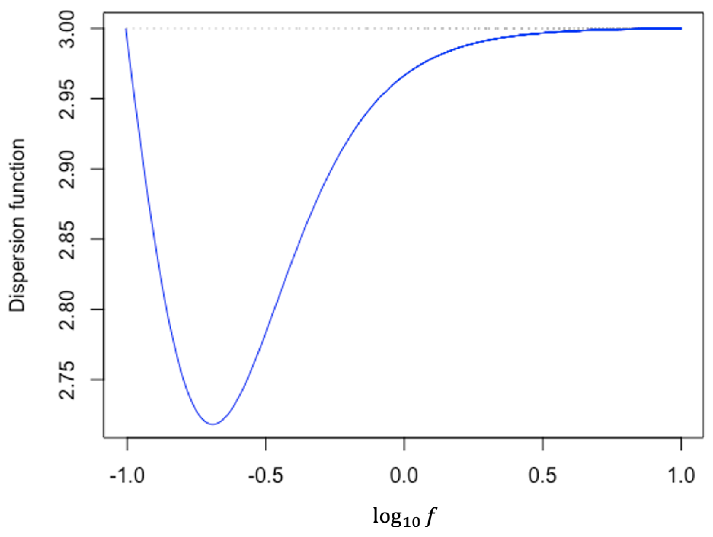
The dispersion function (20), shown in Figure 5, reaches the maximums at the support points (that is, the extremes of the interval) and remains less than 3 (the number of parameters) throughout the design space, so the design obtained is D-optimal.

Figure 6 illustrates the support points of the D-optimal designs obtained with $N=11$ after executing the algorithms and the classic design.

Table 2. Criterion values.

Design	${\mathbf{\Psi }}_{\mathit{D}}\left[\mathit{M}\left({\mathbf{\Phi }}_{\mathit{D}}^{*}\right)\right]$	${\mathit{Eff}}_{\mathit{D}}\left({\mathbf{\Phi }}_{\mathit{D}}\right)$
KL	$2488.52$
REX	$2488.52$
Classic	$1632.01$	$0.65$

shows the values of the D-optimal criterion (19) for the designs obtained from REX, KL and classical. It is observed that the values obtained with the algorithms are greater than the value obtained with the classical design, therefore, the value of the D-optimal criterion has been maximized. Optimal designs are an interesting tool to measure the value of an experimental design, through efficiency. This efficiency is the percentage of observations that the optimal design would need to achieve the precision of the experimental design being compared. The efficiency (22) of the classic design is also presented in Table 2. This shows how the same information can be obtained by reducing the number of experimental conditions by using optimal inputs.

Finally, a sensitivity study has been performed by analysing the fluctuations of the efficiency values against the initial variations of the parameters. In particular, each initial parameter was modified by $\pm 20\%$ of the real values. The efficiencies of the designs obtained have been calculated in relation to the $3^3=27$ possible designs. For all cases, as can be seen from Figure 7, the efficiency for both REX and the KL was never lower than $99.21\%$ and higher than $99.99\%$ for most variations.

5. Conclusions

This paper expands the existing tools to create optimal designs regarding SISO LTI systems in the context of electrical impedance measurements, based on the frequency domain description of an input signal. We have considered the most used optimization criterion, D-optimality. Two algorithms (KL and REX) were modified to calculate D-optimal designs and estimate the parameters of the EEC describing the electrical behaviour of bioelectrodes, cell membranes, or biological tissues. We have checked that the efficiency remains high for different initial values of the parameters. The estimation of the parameters has also been discussed. The application of a sequential approximation with the estimates obtained by means of least squares stabilize the process quickly. We have calculated the D-optimal designs with the same number of points as those of the classical design to obtain an efficiency comparison. It has been seen that optimal designs computed may save 35% of the observations to get the same results as the classic design.

The generation of new results for the design of optimal input signals in impedance models is very useful both in the characterization of biological tissues and the electrode–tissue interface. Specifically, the KL exchange and random exchange REX algorithms that we have adapted are a good option to be used by experimenters to obtain a good estimate of the parameters with lower time-consuming.

References

1. Barsoukov, E.; Macdonald, J.R. Impedance Spectroscopy: Theory, Experiment, and Applications, 3rd ed.; John Wiley and Sons: Hoboken, NJ, USA, 2018. [Google Scholar]
2. Hernández-Balaguera, E.; López-Dolado, E.; Polo, J.L. Obtaining electrical equivalent circuits of biological tissues using the current interruption method, circuit theory and fractional calculus. RSC Adv. 2016, 6, 22312–22319. [Google Scholar] [CrossRef]
3. Hernández-Balaguera, E.; Polo, J.L. On the potential-step hold time when the transient-current response exhibits a Mittag-Leffler decay. J. Electroanal. Chem. 2020, 856, 113631. [Google Scholar]
4. Grimnes, S.; Martinsen, ∅.G. Bioimpedance and Bioelectricity Basics, 3rd ed.; Academic Press: London, UK, 2015. [Google Scholar]
5. Oppenheim, A.V.; Willsky, A.S.; Nawab, H. Signals and Systems, 2nd ed.; Prentice Hall: Upper Saddle Rider, NJ, USA, 1997. [Google Scholar]
6. Ferris, C.D. A General Definition for Impedance. IEEE Trans. Educ. 1964, E-7, 6–8. [Google Scholar] [CrossRef]
7. Ziemer, R.E.; Tranter, W.H. Principles of Communications Systems: Modulation, and Noise, 7th ed.; John Wiley and Sons: Hoboken, NJ, USA, 2015. [Google Scholar]
8. Kalaba, R.; Spingarn, K. Control, Identification, and Input Optimization, 1st ed.; Plenum Press: New York, NY, USA, 1982. [Google Scholar]
9. Mehra, R.K. Optimal input signals for parameter estimation in dynamic systems-survey and new results. IEEE Trans. Autom. Control 1974, 19, 753–768. [Google Scholar] [CrossRef]
10. Mehra, R.K. Optimal inputs for linear system identification. IEEE Trans. Autom. Control 1974, 19, 192–200. [Google Scholar] [CrossRef]
11. Goodwin, G.C.; Payne, R.L. Dynamic System Identification: Experiment Design and Data Analysis, 1st ed.; Academic Press: New York, NY, USA, 1977. [Google Scholar]
12. Titterington, D.M. Aspects of Optimal Design in Dynamic Systems. Technometrics 1980, 22, 287–299. [Google Scholar] [CrossRef]
13. Rafajlowicz, E. Optimal experiment design for identification of linear distributed-parameter systems: Frequency domain approach. IEEE Trans. Autom. Control 1983, 28, 806–808. [Google Scholar] [CrossRef]
14. Walter, E.; Pronzato, L. Identification of Parametric Models from Experimental Data; Springer: Berlin/Heidelberg, Germany; New York, NY, USA, 1997. [Google Scholar]
15. Zarrop, M.B. Optimal Experiment Design for Dynamic System Identification; Springer: Berlin/Heidelberg, Germany; New York, NY, USA,, 1979. [Google Scholar]
16. Gevers, M. Identification for control. From the early achievements to the revival of experimental design. Eur. J. Control 2005, 11, 335–352. [Google Scholar] [CrossRef]
17. Hjalmarsson, H. From experiment design to closed-loop control. Automatica 2005, 41, 393–438. [Google Scholar] [CrossRef] [Green Version]
18. Ljung, L. System Identification, Theory for the User, 2nd ed.; Prentice Hall: Upper Saddle Rider, NJ, USA, 1999. [Google Scholar]
19. Sanchez, B.; Vandersteen, G.; Bragos, R.; Schoukens, J. Optimal multisine excitation design for broadband electrical impedance spectroscopy. Meas. Sci. Technol. 2011, 22, 1156011. [Google Scholar] [CrossRef]
20. Sanchez, B.; Rojas, C.R.; Vandersteen, G.; Bragos, R.; Schoukens, J. On the calculation of the D-optimal multisine excitation power spectrum for broadband impedance spectroscopy measurements. Meas. Sci. Technol. 2012, 23, 085702. [Google Scholar] [CrossRef]
21. Kwon, H.; Rojas, C.R.; Butkove, S.B.; Sanchez, B. Three-harmonic optimal multisine input power spectrum for bioimpedance identification. Physiol. Meas. 2019, 40, 05NT02. [Google Scholar] [CrossRef] [PubMed]
22. Imhof, L.; Lopez-Fidalgo, J.; Wong, W.K. Efficiencies of optimal approximate designs for small samples. Stat. Neerl. 2001, 55, 301–318. [Google Scholar] [CrossRef]
23. Kay, S.M. Fundamentals of Statistical Signal Processing: Estimation Theory; Prentice Hall: Upper Saddle River, NJ, USA, 1993. [Google Scholar]
24. Kiefer, J.; Wolfowitz, J. Optimum Designs in Regression Problems. Ann. Math. Stat. 1959, 30, 271–294. [Google Scholar] [CrossRef]
25. Karlin, S.; Studden, W.J. Optimal Experimental Designs. Ann. Math. Stat. 1966, 37, 783–815. [Google Scholar] [CrossRef]
26. Fedorov, V.V. Theory of Optimal Experiments; Academic Press: New York, NY, USA, 1972. [Google Scholar]
27. Atwood, C.L. Optimal and Efficient Designs of Experiments. Ann. Math. Stat. 1969, 40, 1570–1602. [Google Scholar] [CrossRef]
28. Atkinson, A.C.; Donev, A.N.; Tobias, R.D. Optimum Experimental Designs, with SAS; Oxford University Press: New York, NY, USA, 2007. [Google Scholar]
29. Harman, R.; Filová, L.; Richtárik, P. A Randomized Exchange Algorithm for Computing Optimal Approximate Designs of Experiments. J. Am. Stat. Assoc. 2020, 115, 348–361. [Google Scholar] [CrossRef] [Green Version]
30. Böhning, D. A Vertex-Exchange-Method in D-optimal Design Theory. Metrika 1986, 33, 337–347. [Google Scholar] [CrossRef]
Figure 1. Electrical circuit model (A) and Nyquist plot (B).
Mathematics 10 00837 g001
Figure 2. Biological tissue and basic EECs for intra- (A), extracellular media (B), cell membrane (C), and electrode-tissue interface (D).
Mathematics 10 00837 g002
Figure 3. Autolab PGSTAT potentiostat/galvanostat equipment (A) connected to the dummy cell (B) containing the EEC.
Mathematics 10 00837 g003
Figure 4. Nyquist plot obtained from the classic design.
Mathematics 10 00837 g004
Figure 5. Dispersion function for the D-optimal design for the EEC shown in Figure 1A. The abscissa axis represents the logarithm of the frequency f ( f = ω / 2 π ).
Mathematics 10 00837 g005
Figure 6. Support points of the D-optimal designs obtained by the adapted algorithms and the classic design. The values on the points obtained with the algorithms (7 and 4) are the number of replicas of each point.
Mathematics 10 00837 g006
Figure 7. Efficiencies of the 27 possible designs.
Mathematics 10 00837 g007