Article

Adaptive Evolutionary Computation for Nonlinear Hammerstein Control Autoregressive Systems with Key Term Separation Principle

by
Faisal Altaf
1,
Ching-Lung Chang
2,
Naveed Ishtiaq Chaudhary
3,*,
Muhammad Asif Zahoor Raja
3,
Khalid Mehmood Cheema
4,
Chi-Min Shu
5 and
Ahmad H. Milyani
6
1
Graduate School of Engineering Science and Technology, National Yunlin University of Science and Technology, 123 University Road, Section 3, Douliou, Yunlin 64002, Taiwan
2
Department of Computer Science and Information Engineering, National Yunlin University of Science and Technology, 123 University Road, Section 3, Douliou, Yunlin 64002, Taiwan
3
Future Technology Research Center, National Yunlin University of Science and Technology, 123 University Road, Section 3, Douliou, Yunlin 64002, Taiwan
4
Department of Electrical Engineering, Khwaja Fareed University of Engineering & Information Technology, Rahim Yar Khan 64200, Pakistan
5
Department of Safety, Health, and Environmental Engineering, National Yunlin University of Science and Technology, 123 University Road, Section 3, Douliou, Yunlin 64002, Taiwan
6
Department of Electrical and Computer Engineering, King Abdulaziz University, Jeddah 21589, Saudi Arabia
*
Author to whom correspondence should be addressed.
Submission received: 17 February 2022 / Revised: 10 March 2022 / Accepted: 18 March 2022 / Published: 21 March 2022

Abstract

:
The knacks of evolutionary and swarm computing paradigms have been exploited to solve complex engineering and applied science problems, including parameter estimation for nonlinear systems. The population-based computational heuristics applied for parameter identification of nonlinear systems estimate the redundant parameters due to an overparameterization problem. The aim of this study was to exploit the key term separation (KTS) principle-based identification model with adaptive evolutionary computing to overcome the overparameterization issue. The parameter estimation of Hammerstein control autoregressive (HC-AR) systems was conducted through integration of the KTS idea with the global optimization efficacy of genetic algorithms (GAs). The proposed approach effectively estimated the actual parameters of the HC-AR system for noiseless as well as noisy scenarios. The simulation results verified the accuracy, convergence, and robustness of the proposed scheme. While consistent accuracy and reliability of the designed approach was validated through statistical assessments on multiple independent trials.

1. Introduction

Parameter estimation is an essential and fundamental step for solving various engineering and applied science problems [1,2,3]. Parameter estimation and control of nonlinear systems is a challenging task and has been explored in various studies [4,5,6,7]. Nonlinear systems/processes can be modeled through block structure representation, i.e., Hammerstein, Wiener, and Hammerstein–Wiener models [8,9,10]. The Hammerstein model representation given in Figure 1 consists of two blocks where the first block normally represents the static nonlinearity, while the second block is a linear dynamical subsystem [11]. The Hammerstein structure has been used to model different nonlinear processes. For instance, joint stiffness dynamics [12], heating process [13], cascade water tanks [14], geochemical problems [15], pneumatic muscle actuator [16], financial analysis [17], electric load forecasting [18], and muscle dynamics [19,20].
The research community proposed various algorithms/methods for parameter estimation for the Hammerstein model owing to its significance in modeling different nonlinear systems: for example, gradient/least squares iterative methods [21,22,23,24,25], fractional gradient based adaptive strategies [26,27,28,29], Newton iterative scheme [30], Kalman filtering [31], reframed model [32], filtering technique [33], separable block approach [34], Levenberg–Marquardt optimization [35], orthogonal matching pursuit technique [36], and the maximum likelihood scheme [37]. The biological/nature-inspired computations through evolutionary/swarm optimization were also explored for Hammerstein system identification. For instance, Mehmood et al. exploited the strength of genetic algorithms (GA), differential evolution, pattern search, simulated annealing, and backtracking search optimization heuristics for Hammerstein structure identification [38,39,40]. Tariq et al. exploited the maximum likelihood-based adaptive DE for nonlinear system identification [41]. Raja et al. presented a detailed study of applying GAs to the Hammerstein control autoregressive (HC-AR) structure [42]. In [42], the identification of the HC-AR system through GAs was done through an overparameterization approach by making the system linear in parameters which causes the estimation of redundant parameters rather than identifying only the actual parameters of the HC-AR system.
In order to avoid the redundant parameters involved in the overparameterization identification approach used in genetic algorithms, we integrated the key term separation (KTS) principle with the evolutionary computing paradigm of a GA that allowed us to estimate only the actual parameters of the HC-AR system. The KTS principle identifies and separates the key term in the HC-AR identification model [43] and then exploits the global search competency of GAs to estimate only the actual parameters of the system. The performance of the proposed KTS-based scheme was assessed in terms of accuracy, convergence, robustness, consistency, and reliability for varying parameters of the proposed scheme. The main contributions of the proposed study are as follows:
  • A global search identification scheme through the integration of key term separation, KTS principle identification model with the evolutionary computing algorithm of GA is presented for parameter estimation of Hammerstein nonlinear systems.
  • The proposed scheme avoids identifying redundant parameters and effectively estimates only the actual parameters of Hammerstein control autoregressive (HC-AR) systems through minimizing the mean square error-based criterion function.
  • The accuracy, robustness, and convergence of the proposed approach is established through optimal values of estimation-error-based evaluation metrics.
  • The stability and reliability of the designed approach is ascertained through statistical inferences obtained after executing multiple independent trials of the scheme.
The remaining article is organized as follows: Section 2 provides the proposed key term separation-based identification model for HC-AR systems. Section 3 presents the evolutionary computing approach of GAs for the KTS-based identification model of HC-AR systems. Section 4 gives the results of numerical experimentation with elaborative discussion. Section 5 concludes the findings of the study and lists future research directions.

2. Key Term Separation Identification Model

The block diagram of the HC-AR system is given in Figure 1 while mathematically represented as [43,44]
h ( t ) = E ( z ) F ( z ) g ¯ ( t ) + 1 F ( z ) d ( t )
where h(t), g(t), and d(t) represent input, output, and disturbance signal, respectively, while g ¯ ( t ) is a nonlinear function of known basis and written as
g ¯ ( t ) = k 1 μ 1 [ g ( t ) ] + k 2 μ 2 [ g ( t ) ] + + k p μ p [ g ( t ) ]
E(z) and F(z) are defined as
E ( z ) = e 0 + e 1 z 1 + e 2 z 2 + , , + e n e z n e ,
F ( z ) = 1 + f 1 z 1 + f 2 z 2 + , , + f n f z n f
Rearrange Equation (1) as
h ( t ) = ( 1 F ( z ) ) h ( t ) + E ( z ) g ¯ ( t ) + d ( t )
while using Equations (2)–(4) in Equation (5) and assuming e 0 = 1 . Apply the key term separation (KTS) principle by considering g ¯ ( t ) as a key term
h ( t ) = i = 1 n f f i [ h ( t i ) ] + i = 0 n e e i [ g ¯ ( t i ) ] + d ( t ) = i = 1 n f f i [ h ( t i ) ] + e 0 [ g ¯ ( t ) ] + i = 1 n e e i [ g ¯ ( t i ) ] + d ( t ) = i = 1 n f f i [ h ( t i ) ] + i = 1 n e e i [ g ¯ ( t i ) ] + i = 1 p k i μ i [ g ( t ) ] + d ( t )
Write Equation (6) in terms of information and parameter vectors as
h ( t ) = α f T ( t ) f + α e T ( t ) e + μ T ( t ) k + d ( t )
where the information vectors are defined as
α f ( t ) = [ h ( t 1 ) , h ( t 2 ) , , h ( t n f ) ] T n f ,
α e ( t ) = [ g ¯ ( t 1 ) , g ¯ ( t 2 ) , , g ¯ ( t n e ) ] T n e ,
μ ( t ) = [ μ 1 [ g ( t ) ] , μ 2 [ g ( t ) ] , , μ p [ g ( t ) ] ] T p ,
and the corresponding parameter vectors are
f = [ f 1 , f 2 , , f n f ] T n f ,
e = [ e 1 , e 2 , , e n e ] T n e ,
k = [ k 1 , k 2 , , k p ] T p ,
Equations (7)–(13) represent the KTS identification model for HC-AR systems that avoids the estimation of redundant parameters due to the overparameterization approach.

3. Proposed Methodology for KTS System Model

The proposed methodology for parameter estimation of the KTS-based identification model of HC-AR systems was developed in two phases. First, the objective/fitness function was formulated for the KTS model of the HC-AR system presented in Section 2. Second, the HC-AR system was identified through estimating the actual parameters of the HC-AR system using optimization knacks of the evolutionary computing paradigm of a GA. The overall flow diagram of the proposed study in terms of fundamental compartments is provided in Figure 1.

3.1. Fitness Function Formulation

The iterative and recursive identification approaches for parameter estimation of nonlinear systems develop the identification model by expressing the system output as a product of information and parameter vectors [23]. However, the population-based stochastic computing techniques have no such requirement. The fitness function for a GA based on an evolutionary computing paradigm is formulated by exploiting the strength of approximation theory in mean square error sense as
δ = 1 N j = 1 N [ h ( t j ) h ^ ( t j ) ] 2 ,
where N represents the number of samples involved in the parameter identification of HC-AR systems. The desired response h is calculated using Equation (7) while the estimated response is given by the following:
h ^ ( t ) = α f T ( t ) f ^ + α e T ( t ) e ^ + μ T ( t ) k ^ ,
The estimated parameter is written as
θ ^ = [ f ^ , e ^ , k ^ ] ,
where
f ^ = [ f ^ 1 , f ^ 2 , , f ^ n f ] T n f ,
e ^ = [ e ^ 1 , e ^ 2 , , e ^ n e ] T n e ,
k ^ = [ k ^ 1 , k ^ 2 , , k ^ p ] T p ,
Now the objective was to estimate the parameters of the HC-AR system through minimizing the fitness of Equation (14) using a GA-based evolutionary computing approach such that the desired response given by Equation (7) approached the estimate calculated from Equation (15).

3.2. Optimization Procedure: Evolutionary Computing Paradigm

The legacy of global optimization knacks of genetic algorithms (GAs) belongs to a class of evolutionary computational paradigm that is narrated here which is used for learning the parameters of the HC-AR system as portrayed in the fitness function in Equation (14).
The GAs were introduced in a pioneer work conducted by Holland to mimic an optimization task [45]. Normally, the adaptative performance of GAs to find the appropriate candidate solution in a large search dimension is controlled by a reproduction mechanism consisting of the feasible selection of individuals in the nest population, viable crossover operation for the offspring generation, and the diversity maintenance procedure of mutation. GAs were implemented since their introduction in a variety of research domains such as the viable optimization of closed-loop supply chain design [46], optimization of the weights of neural networks representing the nonlinear singular prediction differential system [47], optimization of electroless NiB coating model [48], optimization of the solar selective absorber design [49], and the crack sensitivity control system for nickel-based laser coating [50]. We were motivated/inspired from these significant applications of GA-based evolutionary computing and used GAs for parameter identification of the HC-AR system.
The process flow structure, in terms of the fundamental steps the Gas used for the optimization of the HC-AR system is shown in Figure 2, i.e., representation of the population, fitness-based ranking, selection of the matting pair, crossover procedure, and mutation. A generic process workflow in the form of a block structure is portrayed in Figure 2 for the GAs that were used for the optimization mechanism of the HC-AR system. The simulation and experimentation of GAs was conducted with the help of the invoking routines/program/tools of optimization available in the MATLAB toolbox for optimization while Windows 10 was used as an operating system. The necessary details of GAs with their implementation procedure is given in pseudocode as provided in Algorithm 1.
Algorithm 1: Pseudocode of evolutionary computing with GAs for HC-AR system identification.
Start: Evolutionary computing of genetic algorithms (GAs)
Inputs: Chromosomes or individual representation as follows:
θ = [ θ f , θ e , θ k ] = [ ( f 1 , f 2 , , f n f )       ( e 1 , e 2 , , e n e )       ( k 1 , k 2 , , k n k ) ]
    Population for an ensemble of chromosomes or individuals is given as
P = [ θ 1 θ 2 θ l ] = [ ( f 1 , 1 , f 2 , 1 , , f n f , 1 ) ( e 1 , 1 , e 2 , 1 , , e n e , 1 ) ( k 1 , 1 , k 2 , 1 , , k n k , 1 ) ( f 1 , 2 , f 2 , 2 , , f n f , 2 ) ( e 1 , 2 , e 2 , 2 , , e n e , 2 ) ( k 1 , 2 , k 2 , 2 , , k n k , 2 ) ( f 1 , l , f 2 , l , , f n f , l ) ( e 1 , l , e 2 , l , , e n e , l ) ( k 1 , l , k 2 , l , , k n k , l ) ] ,
  for l members in θ in P
Output: Global Best θ in P
BeginGAs
  //Initialize
  Arbitrarily formulate θ with bounded pseudo real numbers.
  A group of l number of θ represents initial P.
  //Termination/Stoppage Criteria
  Set stoppage of execution of GAs for the following conditions:
    Desire fitness attained i.e., δ → 10−16,
    Fitness function-Tolerance attained i.e., TolFun → 10−20,
    Constrained-Tolerance attained, i.e., TolCon → 10−20,
    Set total number of generations = 600,
    Other default of GA routine in optimization toolbox
  //Main loop of GA
  While {until termination conditions attained} do %
    //Fitness calculation step
    Evaluate δ using Expression (14) and repeat the procedure for each θ in P
    //Check for termination requirements
    If any of termination level attained then go out of the while loop
    else continues
    //Ranking of individual step
    Rank each θ on the basis of quality of fitness θ achieved.
    //Reproduction step through GA operators
    Appropriate/suitable invoking for
    selection (Stochastic uniform via routine ‘@selectionstochunif’),
    crossover (heuristics via rountine ‘@crossoverheuristic’),
    mutations (adaptive feasible via routine ‘@mutationadaptfeasible’)
    Elitism operations up to 5%, i.e., elitism count set as 26 best ranking
    individuals in the population P
    Modify/update P and go to fitness calculation step
  End
  //Storage step of GAs outcomes
  Store the global best θ with credentials of fitness attained, time spent,
  generations exectuted and fitness function counts of the algorithm.
EndGAs
StatisticalAnalysis:
Dataset generation for the statistical observation by repetition of GAs for a sufficiently large number of multiple execution to identify the parameters of the HC-AR and analysis of these datasets was performed for exhaustive assessments.

3.3. Evaluation Metrics

In order to assess the performance of the evolutionary computing paradigm for parameter estimation of nonlinear systems through the KTS-based identification model of HC-AR systems, we defined three evaluation metrics. The formulated assessment criterions are mean square error based on the difference between the responses, i.e., ( MSE ) h ; as given in Equation (14), mean square error based on the difference between the desired and the estimated parameters, i.e., ( MSE ) θ ; and the normalized parameter deviation, i.e., NPD.
( MSE ) θ = mean ( θ θ ^ ) 2 ,
NPD = θ θ ^ θ
where · denote the 2-norm of a vector.

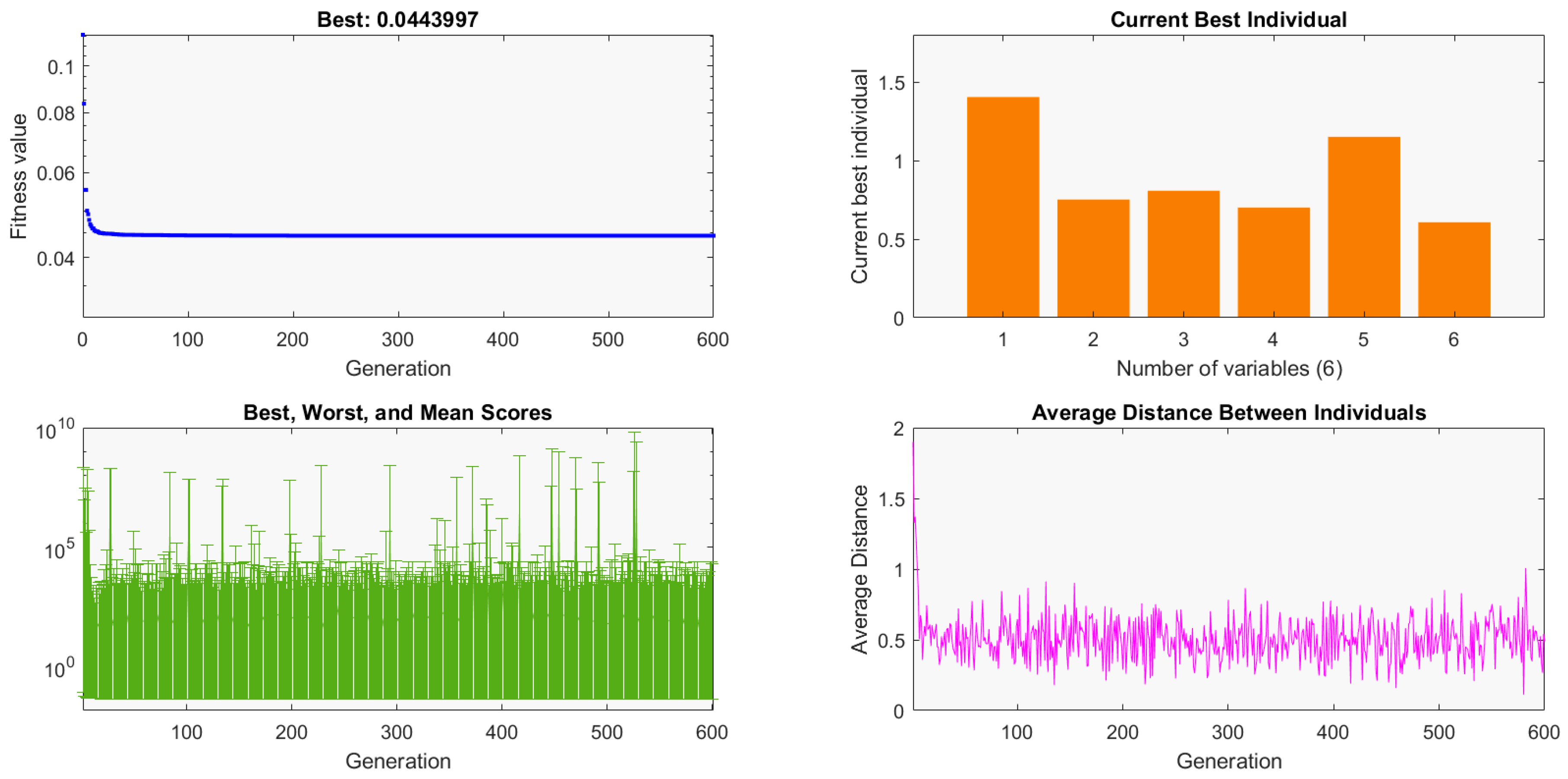
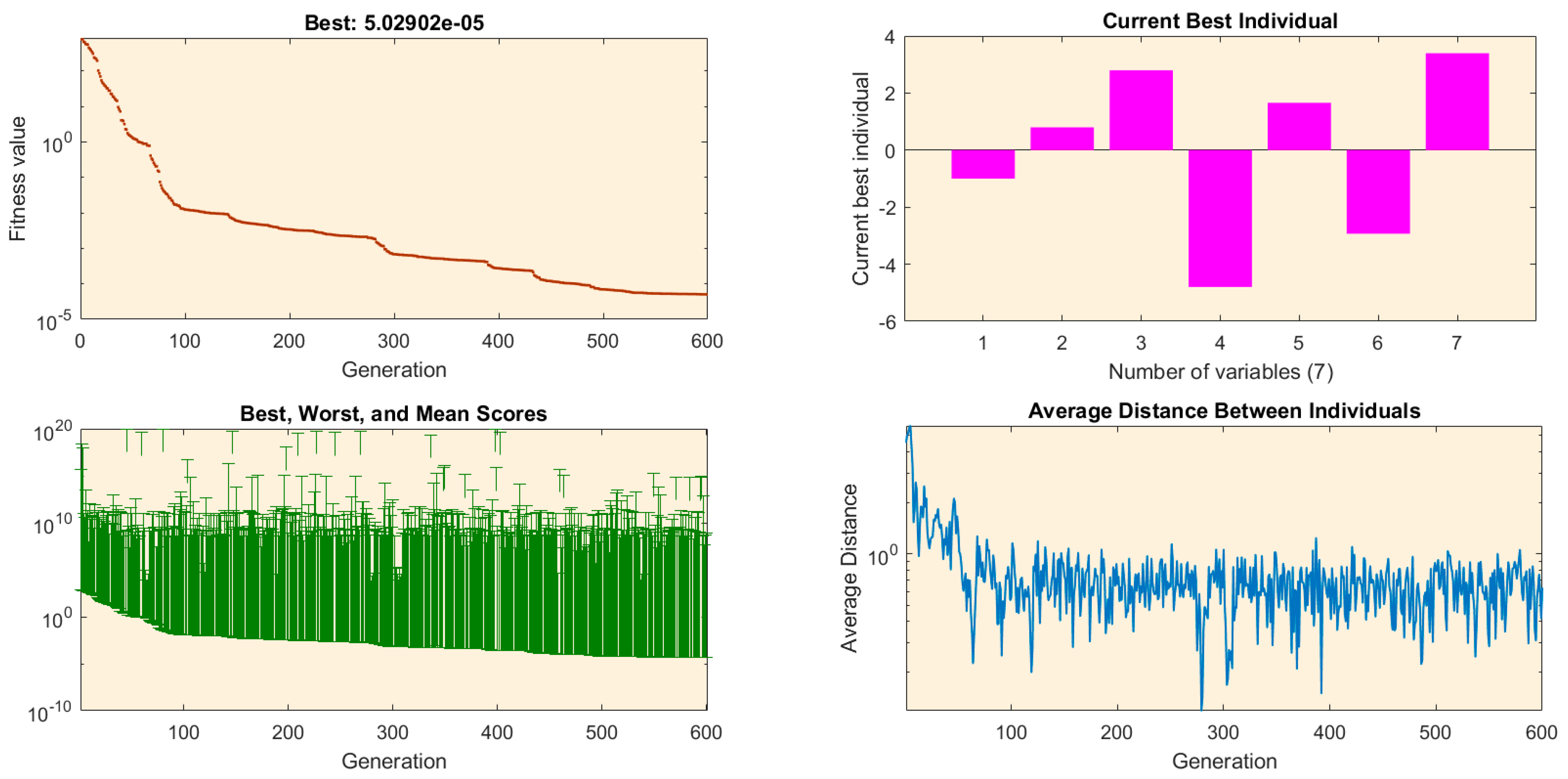
4. Results of Numerical Experimentation with Discussion

The results of the numerical experimentation for parameter estimation for two HC-AR systems are presented in this section. In problem 1, a standard HC-AR system was considered, while in problem 2, a practical application of an HC-AR system representing the dynamics of stimulated muscle model was considered.

4.1. Problem 1

In Problem 1, the HC-AR system was considered with the following parameters, as taken from recent relevant studies to demonstrate the effectiveness of the proposed schemes:
h ( t ) = E ( z ) F ( z ) g ¯ ( t ) + 1 F ( z ) d ( t ) , F ( z ) = 1 + 1.6 1 z 1 + 0.8 z 2 , E ( z ) = 0.85 z 1 + 0.65 z 2 , g ¯ ( t ) = k 1 μ 1 [ g ( t ) ] + k 2 μ 2 [ g ( t ) ] = 1.0 g ( t ) + 0.5 g 2 ( t )
The actual parameters of the HC-AR system were
θ = [ f , e , k ] T = [ f 1 ,   f 2 ,   e 1 ,   e 2   k 1 ,   k 2 ] T = [ θ 1 ,   θ 2 ,   θ 3 ,   θ 4 ,   θ 5 ,   θ 6 ] T = [ 1.6 ,   0.8 ,   0.85 ,   0.65 ,   1 ,   0.5 ] T
Simulations were performed in MATLAB 2020b running on an Asuspro Laptop core i7 with 16GB RAM. The input g was randomly generated with characteristics of zero-mean and unit variance. The disturbance signal was generated with characteristics of Gaussian distribution having zero-mean and constant variance. The robustness of the proposed scheme was assessed for three disturbance levels, i.e., 0, 0.01, and 0.1. The parameter settings of the GA used in the simulations are given in Algorithm 1. The performance of the proposed scheme was deeply investigated through the results of executing a single random run, the statistics through multiple autonomous trials, and evaluating the results for the three different evaluation metrics described in Section 3.3.
The results of the proposed scheme generated for a single random run based on evaluation criteria from Equation (14) in terms of learning curve, best individual scores (best, worst, and mean), and average distance between individuals are provided in Figure 3, Figure 4 and Figure 5 for 0, 0.01, and 0.1 noise levels, respectively. The results indicated that the proposed identification scheme accurately estimated the parameters of the HC-AR system by optimizing the cost function through minimizing the error between the desired and the estimated responses.
The one good run of the evolutionary approach does not guarantee consistently accurate performance. The identification of the HC-AR system through the proposed scheme was also investigated for multiple autonomous executions, and the results are given in Figure 6 and Figure 7 for standard and ascending order, respectively, in the case of all three evaluation metrics. The results verified the consistently accurate performance of the proposed methodology for 70 autonomous trials in the case of all three evaluation metrics given in Equations (14), (20) and (21).
The stability of the design approach was assessed through statistical measurements of the best, mean, and standard deviation. The results of the statistical indices are presented in Table 1 for all considered disturbances and evaluation metrics. The mean values for evaluation criteria (14) were 7.4405 × 10⁻⁷, 3.0590 × 10⁻⁴, and 1.7138 × 10⁻² for disturbance level 0, 0.001, and 0.1, respectively, while the respective mean values in the case of evaluation measures (20) and (21) were 8.0612 × 10⁻⁶, 2.8981 × 10⁻³, 1.4764 × 10⁻¹ and 2.0806 × 10⁻³, 4.7970 × 10⁻², 3.6962 × 10⁻¹, respectively. For a better interpretation, the statistical results are also given in Figure 8. It was witnessed that the proposed scheme consistently provided the accurate results for all considered disturbance levels in the HC-AR system (22). However, the precision level decreased with an increase in disturbance level. The statistical results endorsed the stability, consistently accurate performance, robustness, and reliability of the proposed scheme.
The comparison of the actual parameters of the HC-AR system (22) with the estimated parameters through the proposed scheme was conducted, and the results are presented in Figure 9 and Table 2 along with the actual system parameters. The results validated the accurate and convergent performance of the proposed scheme in estimating the parameters of the HC-AR system (22) for different evaluation measurements based on mean square error of the responses (14), mean square error of the parameters (20), and normalized parameter deviation (21).
While comparing the proposed scheme with the conventional evolutionary approaches [42], the KTS-based GA was more efficient than the conventional GA presented in [42] for the HC-AR identification in the sense that it avoided the estimation of redundant parameters and estimated only the actual parameters of the HC-AR system, thus, making it computationally more efficient than the conventional GA.

4.2. Problem 2

In Problem 2, a practical application of an HC-AR system representing the muscle dynamics required to restore the functional use of paralyzed muscles through automatically controlled stimulations was considered by taking the actual parameters from the real time experimentations performed in the rehabilitation center of the Southampton University [51].
h ( t ) = E ( z ) F ( z ) g ¯ ( t ) + 1 F ( z ) d ( t ) , F ( z ) = 1 z 1 + 0.8 z 2 , E ( z ) = 2.8 z 1 4.8 z 2 , g ¯ ( t ) = k 1 μ 1 [ g ( t ) ] + k 2 μ 2 [ g ( t ) ] = 1.68 g ( t ) 2.88 g 2 ( t ) + 3.42 g 3 ( t )
The actual parameters of the HC-AR system representing the dynamics of the stimulated muscle model are
θ = [ f , e , k ] T = [ f 1 ,   f 2 ,   e 1 ,   e 2   k 1 ,   k 2 ,   k 3 ] T = [ θ 1 ,   θ 2 ,   θ 3 ,   θ 4 ,   θ 5 ,   θ 6 ,   θ 7 ] T = [ 1.0 ,   0.8 ,   2.8 ,   4.8 ,   1.68 ,   2.88 ,   3.42 ] T
In this problem, the same input and disturbance signal were considered as taken from Problem 1. The robustness of the proposed scheme in Problem 2 was assessed for three disturbance levels, i.e., 0, 0.001, and 0.01.
The results of the proposed scheme for Problem 2 of the HC-AR system (23) generated from a single random run based on the evaluation criteria off Equation (14) in terms of learning curve, best individual scores (best, worst, and mean), and average distance between individuals are provided in Figure 10, Figure 11 and Figure 12 for 0, 0.001, and 0.01 noise levels, respectively. The results indicated that the proposed identification scheme accurately estimated the parameters of the HC-AR system (23) by optimizing the cost function through minimizing the error between the desired and the estimated responses.
The comparison of the actual parameters of the HC-AR system (23) with the estimated parameters through the proposed scheme was conducted, and the results based on the best run are presented in Figure 13 and Table 3 along with the actual system parameters. The results validated the accurate and convergent performance of the proposed scheme in estimating the parameters of the muscle model represented through the HC-AR system (23) for different evaluation measures based on the mean square error of the responses (14), the mean square error of the parameters (20), and the normalized parameter deviation (21). This case study presented a KTS-based GA approach for parameter estimation of an HC-AR system representing the parameters of muscle dynamics, while the details for the real rehabilitation procedure can be seen in [51].

5. Conclusions

The conclusions drawn from the study are
  • The integration of an evolutionary computing paradigm of genetic algorithms, GA, with a key term separation-based identification model was presented for parameter estimation of Hammerstein control autoregressive (HC-AR) systems.
  • The proposed identification scheme effectively estimated only the actual parameters of the HC-AR system without estimating the redundant parameters due to an overparameterization approach.
  • The accurate and convergent behavior of the proposed strategy was ascertained through achieving an optimal value of different evaluation metrics based on response error and parameter estimation error.
  • The results of the Monte Carlo simulations and statistical indices established the consistent accuracy of the proposed scheme.
  • The accurate estimation of HC-AR parameters representing the dynamics of a muscle model for the rehabilitation of paralyzed muscles further endorsed the efficacy of the design approach.
The proposed KTS-based evolutionary optimization scheme seems to be an attractive alternative to be exploited for solving complex nonlinear problems [52,53,54,55,56].

Author Contributions

Conceptualization, N.I.C. and M.A.Z.R.; methodology, N.I.C. and M.A.Z.R.; software, F.A.; validation, M.A.Z.R. and N.I.C.; resources, C.-L.C. and C.-M.S.; writing—original draft preparation, F.A.; writing—review and editing, N.I.C. and M.A.Z.R.; project administration, C.-L.C., K.M.C., C.-M.S. and A.H.M.; funding acquisition, K.M.C. and A.H.M. All authors have read and agreed to the published version of the manuscript.

Funding

This research received no external funding.

Institutional Review Board Statement

Not applicable.

Informed Consent Statement

Not applicable.

Data Availability Statement

Not applicable.

Conflicts of Interest

The authors declare no conflict of interest.

References

  1. Bock, H.G.; Carraro, T.; Jäger, W.; Körkel, S.; Rannacher, R.; Schlöder, J.P. (Eds.) Model Based Parameter Estimation: Theory and Applications; Springer Science & Business Media: Berlin/Heidelberg, Germany, 2013; Volume 4. [Google Scholar]
  2. Chaudhary, N.I.; Latif, R.; Raja, M.A.Z.; Machado, J.T. An innovative fractional order LMS algorithm for power signal parameter estimation. Appl. Math. Model. 2020, 83, 703–718. [Google Scholar] [CrossRef]
  3. Ćalasan, M.; Micev, M.; Ali, Z.M.; Zobaa, A.F.; Abdel Aleem, S.H. Parameter Estimation of Induction Machine Single-Cage and Double-Cage Models Using a Hybrid Simulated Annealing—Evaporation Rate Water Cycle Algorithm. Mathematics 2020, 8, 1024. [Google Scholar] [CrossRef]
  4. Billings, S.A.; Leontaritis, I.J. Parameter estimation techniques for nonlinear systems. IFAC Proc. Vol. 1982, 15, 505–510. [Google Scholar] [CrossRef]
  5. Shao, K.; Zheng, J.; Wang, H.; Wang, X.; Liang, B. Leakage-type adaptive state and disturbance observers for uncertain nonlinear systems. Nonlinear Dyn. 2021, 105, 2299–2311. [Google Scholar] [CrossRef]
  6. Fei, J.; Feng, Z. Fractional-order finite-time super-twisting sliding mode control of micro gyroscope based on double-loop fuzzy neural network. IEEE Trans. Syst. Man Cybern. Syst. 2020, 51, 7692–7706. [Google Scholar] [CrossRef]
  7. Fei, J.; Wang, Z.; Liang, X.; Feng, Z.; Xue, Y. Fractional sliding mode control for micro gyroscope based on multilayer recurrent fuzzy neural network. IEEE Trans. Fuzzy Syst. 2021. [Google Scholar] [CrossRef]
  8. Morales, J.Y.R.; Mendoza, J.A.B.; Torres, G.O.; Vázquez, F.D.J.S.; Rojas, A.C.; Vidal, A.F.P. Fault-Tolerant Control implemented to Hammerstein–Wiener model: Application to Bio-ethanol dehydration. Fuel 2022, 308, 121836. [Google Scholar] [CrossRef]
  9. Janczak, A. Identification of Nonlinear Systems Using Neural Networks and Polynomial Models: A Block-Oriented Approach; Springer Science & Business Media: Berlin/Heidelberg, Germany, 2004; Volume 310. [Google Scholar]
  10. Billings, S.A. Nonlinear System Identification: NARMAX Methods in the Time, Frequency, and Spatio-Temporal Domains; John Wiley & Sons: Hoboken, NJ, USA, 2013. [Google Scholar]
  11. Dong, S.; Liu, T.; Wang, Q.G. Identification of Hammerstein systems with time delay under load disturbance. IET Control Theory Appl. 2018, 12, 942–952. [Google Scholar] [CrossRef]
  12. Tehrani, E.S.; Golkar, M.A.; Guarin, D.L.; Jalaleddini, K.; Kearney, R.E. Methods for the identification of time-varying hammerstein systems with applications to the study of dynamic joint stiffness. IFAC-PapersOnLine 2015, 48, 1023–1028. [Google Scholar] [CrossRef]
  13. Hammar, K.; Djamah, T.; Bettayeb, M. Identification of fractional Hammerstein system with application to a heating process. Nonlinear Dyn. 2019, 96, 2613–2626. [Google Scholar] [CrossRef]
  14. Janjanam, L.; Saha, S.K.; Kar, R.; Mandal, D. Improving the Modelling Efficiency of Hammerstein System using Kalman Filter and its Parameters Optimised using Social Mimic Algorithm: Application to Heating and Cascade Water Tanks. J. Frankl. Inst. 2022, 359, 1239–1273. [Google Scholar] [CrossRef]
  15. Piao, H.; Cheng, D.; Chen, C.; Wang, Y.; Wang, P.; Pan, X. A High Accuracy CO2 Carbon Isotope Sensing System Using Subspace Identification of Hammerstein Model for Geochemical Application. IEEE Trans. Instrum. Meas. 2021, 71, 1–9. [Google Scholar] [CrossRef]
  16. Ai, Q.; Peng, Y.; Zuo, J.; Meng, W.; Liu, Q. Hammerstein model for hysteresis characteristics of pneumatic muscle actuators. Int. J. Intell. Robot. Appl. 2019, 3, 33–44. [Google Scholar] [CrossRef]
  17. Tissaoui, K. Forecasting implied volatility risk indexes: International evidence using Hammerstein-ARX approach. Int. Rev. Financ. Anal. 2019, 64, 232–249. [Google Scholar] [CrossRef]
  18. Zhang, Z.; Hong, W.C. Electric load forecasting by complete ensemble empirical mode decomposition adaptive noise and support vector regression with quantum-based dragonfly algorithm. Nonlinear Dyn. 2019, 98, 1107–1136. [Google Scholar] [CrossRef]
  19. Mehmood, A.; Zameer, A.; Chaudhary, N.I.; Raja, M.A.Z. Backtracking search heuristics for identification of electrical muscle stimulation models using Hammerstein structure. Appl. Soft Comput. 2019, 84, 105705. [Google Scholar] [CrossRef]
  20. Mehmood, A.; Zameer, A.; Chaudhary, N.I.; Ling, S.H.; Raja, M.A.Z. Design of meta-heuristic computing paradigms for Hammerstein identification systems in electrically stimulated muscle models. Neural Comput. Appl. 2020, 32, 12469–12497. [Google Scholar] [CrossRef]
  21. Mao, Y.; Ding, F.; Xu, L.; Hayat, T. Highly efficient parameter estimation algorithms for Hammerstein non-linear systems. IET Control Theory Appl. 2019, 13, 477–485. [Google Scholar] [CrossRef]
  22. Ding, F.; Chen, H.; Xu, L.; Dai, J.; Li, Q.; Hayat, T. A hierarchical least squares identification algorithm for Hammerstein nonlinear systems using the key term separation. J. Frankl. Inst. 2018, 355, 3737–3752. [Google Scholar] [CrossRef]
  23. Ding, F.; Ma, H.; Pan, J.; Yang, E. Hierarchical gradient-and least squares-based iterative algorithms for input nonlinear output-error systems using the key term separation. J. Frankl. Inst. 2021, 358, 5113–5135. [Google Scholar] [CrossRef]
  24. Shen, B.; Ding, F.; Xu, L.; Hayat, T. Data filtering based multi-innovation gradient identification methods for feedback nonlinear systems. Int. J. Control Autom. Syst. 2018, 16, 2225–2234. [Google Scholar] [CrossRef]
  25. Ding, J.; Cao, Z.; Chen, J.; Jiang, G. Weighted parameter estimation for Hammerstein nonlinear ARX systems. Circuits Syst. Signal Process. 2020, 39, 2178–2192. [Google Scholar] [CrossRef]
  26. Chaudhary, N.I.; Raja, M.A.Z.; He, Y.; Khan, Z.A.; Machado, J.T. Design of multi innovation fractional LMS algorithm for parameter estimation of input nonlinear control autoregressive systems. Appl. Math. Model. 2021, 93, 412–425. [Google Scholar] [CrossRef]
  27. Chaudhary, N.I.; Aslam, M.S.; Baleanu, D.; Raja, M.A.Z. Design of sign fractional optimization paradigms for parameter estimation of nonlinear Hammerstein systems. Neural Comput. Appl. 2020, 32, 8381–8399. [Google Scholar] [CrossRef]
  28. Xu, C.; Mao, Y. Auxiliary Model-Based Multi-Innovation Fractional Stochastic Gradient Algorithm for Hammerstein Output-Error Systems. Machines 2021, 9, 247. [Google Scholar] [CrossRef]
  29. Chaudhary, N.I.; Zubair, S.; Raja, M.A.Z.; Dedovic, N. Normalized fractional adaptive methods for nonlinear control autoregressive systems. Appl. Math. Model. 2019, 66, 457–471. [Google Scholar] [CrossRef]
  30. Li, J. Parameter estimation for Hammerstein CARARMA systems based on the Newton iteration. Appl. Math. Lett. 2013, 26, 91–96. [Google Scholar] [CrossRef] [Green Version]
  31. Ma, J.; Ding, F.; Xiong, W.; Yang, E. Combined state and parameter estimation for Hammerstein systems with time delay using the Kalman filtering. Int. J. Adapt. Control Signal Process. 2017, 31, 1139–1151. [Google Scholar] [CrossRef] [Green Version]
  32. Wang, D. Hierarchical parameter estimation for a class of MIMO Hammerstein systems based on the reframed models. Appl. Math. Lett. 2016, 57, 13–19. [Google Scholar] [CrossRef]
  33. Wang, D.; Zhang, Z.; Xue, B. Decoupled parameter estimation methods for Hammerstein systems by using filtering technique. IEEE Access 2018, 6, 66612–66620. [Google Scholar] [CrossRef]
  34. Zhang, S.; Wang, D.; Liu, F. Separate block-based parameter estimation method for Hammerstein systems. R. Soc. Open Sci. 2018, 5, 172194. [Google Scholar] [CrossRef] [PubMed] [Green Version]
  35. Li, J.; Zheng, W.X.; Gu, J.; Hua, L. Parameter estimation algorithms for Hammerstein output error systems using Levenberg–Marquardt optimization method with varying interval measurements. J. Frankl. Inst. 2017, 354, 316–331. [Google Scholar] [CrossRef]
  36. Mao, Y.; Ding, F.; Liu, Y. Parameter estimation algorithms for Hammerstein time-delay systems based on the orthogonal matching pursuit scheme. IET Signal Process. 2017, 11, 265–274. [Google Scholar] [CrossRef]
  37. Wang, D.Q.; Zhang, Z.; Yuan, J.Y. Maximum likelihood estimation method for dual-rate Hammerstein systems. Int. J. Control Autom. Syst. 2017, 15, 698–705. [Google Scholar] [CrossRef]
  38. Mehmood, A.; Aslam, M.S.; Chaudhary, N.I.; Zameer, A.; Raja, M.A.Z. Parameter estimation for Hammerstein control autoregressive systems using differential evolution. Signal Image Video Process. 2018, 12, 1603–1610. [Google Scholar] [CrossRef]
  39. Mehmood, A.; Chaudhary, N.I.; Zameer, A.; Raja, M.A.Z. Backtracking search optimization heuristics for nonlinear Hammerstein controlled auto regressive auto regressive systems. ISA Trans. 2019, 91, 99–113. [Google Scholar] [CrossRef] [PubMed]
  40. Mehmood, A.; Chaudhary, N.I.; Zameer, A.; Raja, M.A.Z. Novel computing paradigms for parameter estimation in Hammerstein controlled auto regressive auto regressive moving average systems. Appl. Soft Comput. 2019, 80, 263–284. [Google Scholar] [CrossRef]
  41. Tariq, H.B.; Chaudhary, N.I.; Khan, Z.A.; Raja MA, Z.; Cheema, K.M.; Milyani, A.H. Maximum-Likelihood-Based Adaptive and Intelligent Computing for Nonlinear System Identification. Mathematics 2021, 9, 3199. [Google Scholar] [CrossRef]
  42. Raja, M.A.Z.; Shah, A.A.; Mehmood, A.; Chaudhary, N.I.; Aslam, M.S. Bio-inspired computational heuristics for parameter estimation of nonlinear Hammerstein controlled autoregressive system. Neural Comput. Appl. 2018, 29, 1455–1474. [Google Scholar] [CrossRef]
  43. Chaudhary, N.I.; Raja, M.A.Z.; Khan, Z.A.; Cheema, K.M.; Milyani, A.H. Hierarchical Quasi-Fractional Gradient Descent Method for Parameter Estimation of Nonlinear ARX Systems Using Key Term Separation Principle. Mathematics 2021, 9, 3302. [Google Scholar] [CrossRef]
  44. Giri, F.; Bai, E.W. Block-Oriented Nonlinear System Identification, 1st ed.; Springer: London, UK, 2010; Volume 1. [Google Scholar]
  45. Holland, J.H. Genetic algorithms and the optimal allocation of trials. SIAM J. Comput. 1973, 2, 88–105. [Google Scholar] [CrossRef]
  46. Yun, Y.; Chuluunsukh, A.; Gen, M. Sustainable closed-loop supply chain design problem: A hybrid genetic algorithm approach. Mathematics 2020, 8, 84. [Google Scholar] [CrossRef] [Green Version]
  47. Sabir, Z.; Raja, M.A.Z.; Botmart, T.; Weera, W. A Neuro-Evolution Heuristic Using Active-Set Techniques to Solve a Novel Nonlinear Singular Prediction Differential Model. Fractal Fract. 2022, 6, 29. [Google Scholar] [CrossRef]
  48. Vijayanand, M.; Varahamoorthi, R.; Kumaradhas, P.; Sivamani, S.; Kulkarni, M.V. Regression-BPNN modelling of surfactant concentration effects in electroless NiB coating and optimization using genetic algorithm. Surf. Coat. Technol. 2021, 409, 126878. [Google Scholar] [CrossRef]
  49. Wang, Z.Y.; Hu, E.T.; Cai, Q.Y.; Wang, J.; Tu, H.T.; Yu, K.H.; Chen, L.Y.; Wei, W. Accurate design of solar selective absorber based on measured optical constants of nano-thin Cr Film. Coatings 2020, 10, 938. [Google Scholar] [CrossRef]
  50. Yu, J.; Sun, W.; Huang, H.; Wang, W.; Wang, Y.; Hu, Y. Crack sensitivity control of nickel-based laser coating based on genetic algorithm and neural network. Coatings 2019, 9, 728. [Google Scholar] [CrossRef] [Green Version]
  51. Le, F.; Markovsky, I.; Freeman, C.T.; Rogers, E. Recursive identification of Hammerstein systems with application to electrically stimulated muscle. Control Eng. Pract. 2012, 20, 386–396. [Google Scholar] [CrossRef] [Green Version]
  52. Cao, W.; Zhu, Q. Stability of stochastic nonlinear delay systems with delayed impulses. Appl. Math. Comput. 2022, 421, 126950. [Google Scholar] [CrossRef]
  53. Kong, F.; Zhu, Q.; Huang, T. New Fixed-Time Stability Criteria of Time-Varying Delayed Discontinuous Systems and Application to Discontinuous Neutral-Type Neural Networks. IEEE Trans. Cybern. 2021, 1–10. [Google Scholar] [CrossRef]
  54. Aadhithiyan, S.; Raja, R.; Zhu, Q.; Alzabut, J.; Niezabitowski, M.; Lim, C.P. A Robust Non-Fragile Control Lag Synchronization for Fractional Order Multi-Weighted Complex Dynamic Networks with Coupling Delays. Neural Process. Lett. 2022, 1–22. [Google Scholar] [CrossRef]
  55. Kong, F.; Zhu, Q.; Huang, T. Improved Fixed-Time Stability Lemma of Discontinuous System and Its Application. IEEE Trans. Circuits Syst. I Regul. Pap. 2021, 69, 835–842. [Google Scholar] [CrossRef]
  56. Xiao, H.; Zhu, Q. Stability analysis of switched stochastic delay system with unstable subsystems. Nonlinear Anal. Hybrid Syst. 2021, 42, 101075. [Google Scholar] [CrossRef]
Figure 1. Workflow of methodology for HC-AR systems with evolutionary heuristics of GAs.
Mathematics 10 01001 g001
Figure 2. Overview of reproduction operators of GAs representing HC-AR systems.
Mathematics 10 01001 g002
Figure 3. Results of Problem 1 in terms of learning curve, best individual scores, and average distance for no noise scenario.
Mathematics 10 01001 g003
Figure 4. Results of Problem 1 in terms of learning curve, best individual scores, and average distance for 0.01 noise level.
Mathematics 10 01001 g004
Figure 5. Results of Problem 1 in terms of learning curve, best individual scores, and average distance for 0.1 noise level.
Mathematics 10 01001 g005
Figure 6. Results of autonomous executions through different evaluation metrics for Problem 1. (a) MSE through estimated response (b) MSE through estimated parameters (c) Normalized parameter deviation.
Mathematics 10 01001 g006aMathematics 10 01001 g006b
Figure 7. Result of autonomous executions in ascending order through different evaluation metrics for Problem 1. (a) MSE (ascending order) through estimated response (b) MSE (ascending order) through estimated parameters (c) Normalized (ascending order) parameter deviation.
Mathematics 10 01001 g007
Figure 8. Graphic interpretation of statistics for different evaluation metrics in the case of Problem 1. (a) MSE through estimated responses (b) MSE through estimated parameters (c) Normalized parameter deviation.
Mathematics 10 01001 g008aMathematics 10 01001 g008b
Figure 9. Results of estimated parameters in comparison with actual HC-AR parameters considered in Problem 1. (a) MSE through estimated responses (b) MSE through estimated parameters (c) Normalized parameter deviation.
Mathematics 10 01001 g009aMathematics 10 01001 g009b
Figure 10. Results of Problem 2 in terms of learning curve, best individual scores, and average distance for 0 noise level.
Mathematics 10 01001 g010
Figure 11. Results of Problem 2 in terms of learning curve, best individual scores, and average distance for 0.001 noise level.
Mathematics 10 01001 g011
Figure 12. Results of Problem 2 in terms of learning curve, best individual scores, and average distance for 0.01 noise level.
Mathematics 10 01001 g012
Figure 13. Results of estimated parameters in comparison with actual HC-AR parameters considered in Problem 2. (a) MSE through estimated responses (b) MSE through estimated parameters (c) Normalized parameter deviation.
Mathematics 10 01001 g013
Table 1. Results of statistical indices for different evaluation metrics in Problem 1.
NoiseStatistical IndicesMSE ResponsesMSE ParametersNPD
0Minimum1.8583 × 10−142.1427 × 10−173.5541 × 10⁻⁷
Mean7.4405 × 10−178.0612 × 10−62.0806 × 10−3
Standard Deviation2.6148 × 10−63.6142 × 10−55.0126 × 10−3
0.01Minimum4.9615 × 10−56.2525 × 10−58.1884 × 10−3
Mean3.0590 × 10−42.8981 × 10−34.7970 × 10−2
Standard Deviation2.0307 × 10−44.3865 × 10−32.8608 × 10−2
0.1Minimum1.7040 × 10−31.4920 × 10−21.2649 × 10−1
Mean1.7138 × 10−21.4764 × 10−13.6962 × 10−1
Standard Deviation1.3315 × 10−21.1119 × 10−11.4840 × 10−1
Table 2. Comparison of the estimated parameter values with the actual parameters of Problem 1.
MetricNoise θ 1 θ 2 θ 3 θ 4 θ 5 θ 6 Metric Value
MSE01.60000.80000.85000.65001.00000.50002.14 × 10−17
0.011.59340.79720.85340.66141.01010.50896.25 × 10−5
0.11.74680.98280.96780.75251.07910.56261.49 × 10−2
NWD01.60000.80000.85000.65001.00000.50003.55 × 10−7
0.011.59340.79720.85340.66141.01010.50898.19 × 10−3
0.11.74680.98280.96780.75251.07910.56261.26 × 10−1
DW 1.60000.80000.85000.65001.00000.50000
Table 3. Comparison of the estimated parameter values with the actual parameters of Problem 2.
MetricNoise θ 1 θ 2 θ 3 θ 4 θ 5 θ 6 θ 7 Value
MSE0−1.00010.80002.7942−4.79281.6636−2.90943.41554.88 × 10−5
0.001−0.99990.80012.7836−4.77861.7292−2.88843.42514.64 × 10−4
0.01−1.00010.80002.7912−4.79031.6224−2.98803.37952.40 × 10−3
NWD0−1.00010.80002.7942−4.79281.6636−2.90943.41554.73 × 10−3
0.001−0.99990.80012.7836−4.77861.7292−2.88843.42517.66 × 10−3
0.01−1.00010.80002.7912−4.79031.6224−2.98803.37951.74 × 10−2
DW −1.00000.80002.8000−4.80001.6800−2.88003.42000
Publisher’s Note: MDPI stays neutral with regard to jurisdictional claims in published maps and institutional affiliations.

