A Lagrangian DG-Method for Wave Propagation in a Cracked Solid with Frictional Contact Interfaces

Abstract

We developed a discontinuous Galerkin (DG) numerical scheme for wave propagation in elastic solids with frictional contact interfaces. This type of numerical scheme is useful in investigations of wave propagation in elastic solids with micro-cracks (cracked solid) that involve modeling the damage in brittle materials or architected meta-materials. Only processes with mild loading that do not trigger crack fracture extension or the nucleation of new fractures are considered. The main focus lies on the contact conditions at crack surfaces, including provisions for crack opening and closure and stick-and-slip with Coulomb friction. The proposed numerical algorithm uses the leapfrog scheme for the time discretization and an augmented Lagrangian algorithm to solve the associated non-linear problems. For efficient parallelization, a Galerkin discontinuous method was chosen for the space discretization. The frictional interfaces (micro-cracks), where the numerical flux is obtained by solving non-linear and non-smooth variational problems, concerns only a limited number the degrees of freedom, implying a small additional computational cost compared to classical bulk DG schemes. The numerical method was tested through two model problems with analytical solutions. The proposed Lagrangian approach of the nonlinear interfaces had excellent results (stability and high accuracy) and only required a reasonable additional amount of computational effort. To illustrate the method, we conclude with some numerical simulations on the blast propagation in a cracked material and in a meta-material designed for shock dissipation.

1. Introduction

Micro-fractures strongly influence the (seismic) wave propagation that gives rise to scattering and fracture-induced anisotropy. This phenomenon makes the derivation of accurate relationships between the micro-structure (pores, micro-cracks) and overall elastic properties of brittle materials (rocks, ceramics,…) difficult. In a fractured medium, when the dimensions of the fractures are substantially smaller than the wavelength, the wave propagation can be described by using effective-medium theories (see, for instance, [1,2,3,4] or [5] and references therein). However, if the wavelength is of the same order as the micro-cracks’ radii, numerical simulations are the main tool of investigation.

The performances of meta-materials can be explained by their internal architectures involving stiff and strong building blocks bonded by weaker interfaces. These interfaces, which play a crucial role, enable large deformations and energy dissipation mechanisms throughout large volumes of the materials. Moreover, the mechanical behavior of these interfaces, which is typically nonlinear and governed by friction, is strongly related to their morphology (see, for instance, [6]).

A large majority of numerical schemes treating wave propagation in materials with micro-fractures use the finite-difference (FD) method. Some of them take the cracks as secondary point sources [7]. Others use penny-shaped weak inclusions [8,9] to model the micro-cracks. In order to adequately model the thickness of cracks, the finite-difference discretization has to be carried out on a small grid spacing, which generates high computational costs (both the grid spacing and the time interval have to be small to satisfy stability considerations). Additionally, when the medium contains high-contrast discontinuities (strong heterogeneities), some instability problems arise on a staggered grid [10]. Some of them could be avoided by using the rotated staggered grid technique [11].

In contrast, for “explicit interface” approaches the fracture is assumed to have a vanishing width across which tractions are continuous, but displacements and velocities are allowed to have jumps. One of the “explicit interface” approaches is the so-called “linear-slip displacement-discontinuity model” [3,12,13,14] offering a unified description of fractures on scales both large and small, relative to the wavelength. However, this model is linear and cannot describe the nonlinear phenomena present on the micro-cracks’ interface, such as as unilateral contact and/or friction.

To model frictional contact constraints, the classical finite element (FE) technique makes use of two (nodal values) discretization methods: the (augmented) Lagrangian method and the penalty method (see, for instance, [15,16,17,18,19,20,21,22] or [23]). Other discretization schemes, such as mortar methods, were developed for non-matching grids [24,25,26,27]. Another class of mixed formulations encompasses the “dual mortar” methods (see, for instance, [28,29]). An alternative to mixed methods is using the primal formulation (in which the displacement field is the only unknown) by Nitsche’s method (see [30,31] and its extensions to estimate either quasi-static friction [32,33] or explicit dynamics [34]).

Nitsche’s method has also been used under the guise of the “interior penalty” method within the context of discontinuous Galerkin (DG) methods (see Arnold [35] for the earliest applications). There have been a lot of important developments in DG approaches for linear and nonlinear solid mechanics (see, for instance, [36] for linear elasticity developments; [37,38,39] for finite-strain elasticity developments; [40] for elasto-plasticity developments; and [41] for second-order computational homogenization). A unifying analysis of the DG method applied to elliptic problems is contained in [17]. Recently, Truster and Masud [42] developed a stabilized DG interface method for transient contact with Coulomb friction that extends their previous work on interphase damage modeling [43]. To overcome the non-smoothness of the Coulomb friction model, they used an elasto-plastic regularization technique (see Simo and Laursen [18]). This regularization needs a tangential stiffness parameter which is not always simple to capture experimentally. Truster and Masud’s approach is associated with a classical treatment (FE discretization in space and with an implicit Newmark scheme in time) of the elastodynamics equations, while a DG method is used only for the interface nonlinear conditions.

Single and multi-field versions of an h-adaptive, asynchronous space-time discontinuous Galerkin (aSDG) method for elastodynamics, proposed initially in [44,45], were developed by Abedi et al. [46] to simulate dynamic crack propagation with a cohesive model. The aSDG numerical fluxes derive from Riemann solutions of the hyperbolic elastodynamic system, and are therefore more accurate than other fluxes (for instance, the centered flux [47]), but they are restricted to isotropic elasticity. Moreover, Abedi and Haber [48] extend the elastodynamic Riemann fluxes in order to treat interfaces subject to frictional contact constraints and use them to obtain high-resolution aSDG solutions for complex contact problems.

The aim of this study was to develop a robust and accurate (fully) DG method for solving the elasto-dynamics’ equations with nonlinear boundary conditions (as friction and/or contact) on a set of interfaces (as internal micro-cracks for instance). This numerical method can be used to determine the effective properties of the damaged materials via a numerical up-scaling homogenization technique by analyzing the wave propagation (speed, amplitude, wavelength) in a cracked material, as in [49], or to study the dissipation properties of meta-materials that exhibit many frictional interfaces. The applications we have in mind concern brittle materials (as ceramics and rocks), but other elastic materials, such as metals, could also be considered.

The principal original aspects of the proposed numerical scheme lay in the interplay between the leapfrog scheme for the time discretization and the augmented Lagrangian algorithm for solving the associated non-linear problems. Concerning the space discretization, a Galerkin discontinuous method was chosen for its accuracy and efficient parallelization of the computations. Even if for the bulk elements several choices of the numerical flux could be made, the centered flux was preferred for the numerical implementation. The flux in micro-cracks boundaries is computed by solving two non-linear and non-smooth variational problem without any regularization technique. In this way the interfaces’ conditions are modeled simply by different flux choices for the adjacent elements without any specific geometric treatment of the micro-cracks. Since the proposed (augmented) Lagrangian algorithm is related only to the interfaces’ degrees of freedom, the additional computational effort in modeling the nonlinear interfaces is not important.

Let us outline the content of the paper. The elastodynamics problem in a domain with interfaces (cracks) in frictional unilateral contact is stated in Section 2, whereas in Section 3 the proposed numerical method is introduced. The leapfrog time discretization splits the elastodynamics problem into two problems: velocity and stress problems. After that, the nonlinear boundary conditions are written as two variational inequalities involving fluxes at the interfaces (micro-cracks). The unilateral condition is associated with the velocity problem, and the friction law relates to the stress problem. By using the DG method for space discretization, the bulk elements are independent of the contact interfaces, which means that classical choices of the flux can be made. However, the fluxes on the interfaces, related to the two nonlinear variational inequalities, have to be found through a numerical iterative algorithm, such as the (augmented) Lagrangian approach. In Section 4, the numerical method was tested (stability, mesh and time step sensitivity) through two model problems for which analytical solutions exist. Finally, we illustrate how our DG method may be used to investigate more complex wave propagation phenomena, such as blast-wave propagation in a ceramic block with an anisotropic crack distribution.

2. Problem Statement

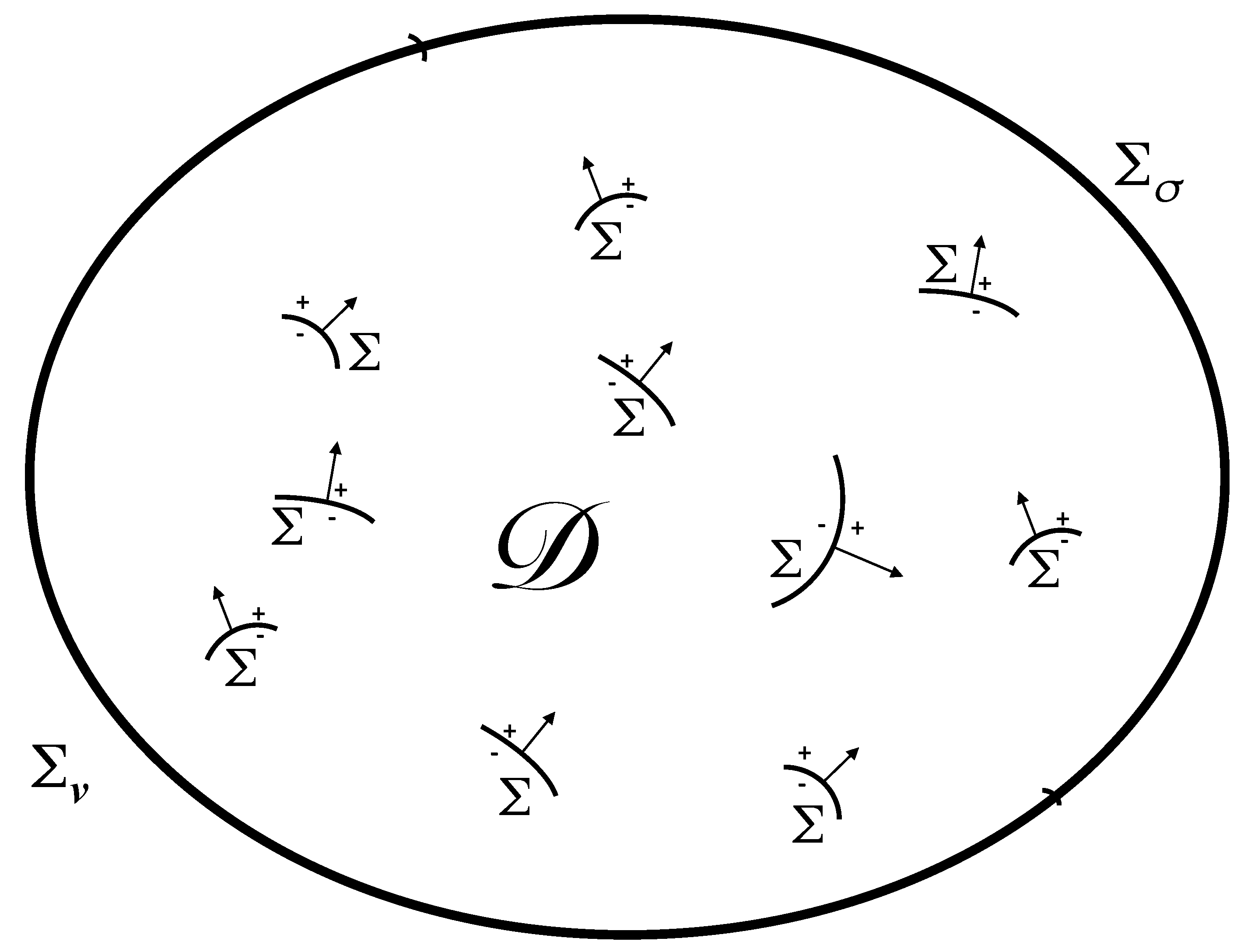
Let $\mathcal{D}\subset {\mathbb{R}}^3$ be an elastic domain which contains a set of interfaces on its boundary. To model a cracked solid, these interfaces (a set of micro-cracks) are located on the internal boundary $\Sigma \subset \mathring{\overline{\mathcal{D}}}$ (see Figure 1 for a schematic representation), but other configurations could also be considered. We are looking for the displacement $\mathit{u}:[0,T]\times \mathcal{D}\to {\mathbb{R}}^3$ and the stress tensor $\mathit{\sigma }:[0,T]\times \mathcal{D}\to {\mathbb{R}}_s^{3\times 3}$ (here ${\mathbb{R}}_s^{3\times 3}$ is the space of symmetric $3\times 3$ matrices) solution of the following equations:

$$\begin{array}{cccccccc}\hfill \mathit{\rho }\ddot{\mathit{u}}(t)& =\mathrm{div}\mathit{\sigma }(t)+\mathit{\rho }\mathit{b}(t)\hfill & & & & & & \hfill \mathrm{in}\mathcal{D},\end{array}$$

(1)

$$\begin{array}{cccccccc}\hfill \mathit{\sigma }& =\mathcal{E}\mathit{\epsilon }\hfill & & & & & & \hfill \mathrm{in}\mathcal{D},\end{array}$$

(2)

$$\begin{array}{cccccccc}\hfill \mathit{\epsilon }(\mathit{u})& =\frac{1}{2}(\nabla \mathit{u}+{\nabla }^t\mathit{u})\hfill & & & & & & \hfill \mathrm{in}\mathcal{D},\end{array}$$

(3)

where $\mathit{\epsilon }$ is the small strain tensor, $\mathit{\rho }\mathit{b}$ are the volume forces and $\mathcal{E}$ is the fourth order tensor of elastic coefficients. If we denote by $\mathit{v}=\dot{\mathit{u}}$ the velocity field and by $\mathcal{A}={\mathcal{E}}^{-1}$ the compliance tensor, then (2) reads

$$\mathcal{A}\dot{\mathit{\sigma }}(t)=\mathit{\epsilon }(\mathit{v}(t)).$$

(4)

Let n be the normal $\Sigma$-oriented from − to + sides as defined on Figure 1. We define the jump $[\mathit{\phi }]$ of $\mathit{\phi }$ by the difference ${\mathit{\phi }}^{+}-{\mathit{\phi }}^{-}$. The boundary $\partial \mathcal{D}$ of $\mathcal{D}$ will be divided into two parts: the internal boundary $\Sigma$, and the “loading” boundary, which is the union of two disjoints parts ${\Sigma }_v$ and ${\Sigma }_{\sigma }$, i.e., $\partial \mathcal{D}=\Sigma \cup {\Sigma }_v\cup {\Sigma }_{\sigma }$. On the external boundary ${\Sigma }_v\cup {\Sigma }_{\sigma }$ we impose the displacement and the stress vector:

$$\begin{array}{c}\hfill \mathit{u}(t)=\mathit{U}(t)\mathrm{on}{\Sigma }_v,\mathit{\sigma }\mathit{n}(t)={\mathit{F}}_s(t)\mathrm{on}{\Sigma }_{\sigma },\end{array}$$

(5)

while on the internal boundary $\Sigma$ we consider unilateral contact conditions with Coulomb friction.

The non-penetration Signorini conditions read

$$[\mathit{\sigma }]=0\mathrm{on}\Sigma ;[\mathit{u}]·\mathit{n}⩾0;{\sigma }_n⩽0;{\sigma }_n([\mathit{u}]·\mathit{n})=0,\mathrm{on}\Sigma ,$$

(6)

while

$$|{\mathit{\sigma }}_T|+{\mu }_f{\sigma }_n⩽0,(|{\mathit{\sigma }}_T|+{\mu }_f{\sigma }_n)[{\dot{\mathit{u}}}_T]=0\mathrm{and}{\displaystyle \frac{[{\dot{\mathit{u}}}_T]}{|[{\dot{\mathit{u}}}_T]|}}=-{\displaystyle \frac{{\mathit{\sigma }}_T}{|{\mathit{\sigma }}_T|}},$$

(7)

represent the (isotropic) Coulomb friction conditions, with ${\mu }_f$ being the Coulomb coefficient. We have used here the normal and tangential decomposition ${\sigma }_n=(\sigma \mathit{n})·\mathit{n}$, ${\mathit{\sigma }}_T=\sigma \mathit{n}-{\sigma }_n\mathit{n},{\mathit{u}}_T=\mathit{u}-(\mathit{u}·\mathit{n})\mathit{n}$.

Let us write the Coulomb friction law (7) as a variational inequality. This will be useful in developing the numerical approach. For that, let us consider the set of admissible stresses

$$\begin{array}{cc}\hfill {\mathcal{S}}^t& =\{\mathit{\tau }:\mathcal{D}\to {\mathbb{R}}_s^{3\times 3};[\mathit{\tau }]\mathit{n}=0,|{\mathit{\tau }}_T|+{\mu }_f{\sigma }_n(t)⩽0\mathrm{on}\Sigma \}.\hfill \end{array}$$

(8)

Then (7) is equivalent with

$$\mathit{\sigma }(t)\in {\mathcal{S}}^t;{[\dot{\mathit{v}}(t)]}_T·({\mathit{\tau }}_T-{\mathit{\sigma }}_T(t))⩽0\mathrm{for}\mathrm{all}\tau \in {\mathcal{S}}^t$$

(9)

We complete the field equations and the boundary conditions with the initial conditions

$$\mathit{u}(0)={\mathit{u}}_0(\mathrm{or}\mathit{\sigma }(0)={\mathit{\sigma }}^0=\mathcal{A}\mathit{\epsilon }({\mathit{u}}_0)),\mathit{v}(0)={\mathit{v}}^0,\mathrm{in}\mathcal{D}.$$

(10)

The initial and boundary problem can be formulated now as follows: Find the displacement $\mathit{u}:[0,T]\times \mathcal{D}\to {\mathbb{R}}^3$ (or equivalently the velocity $\mathit{v}=\dot{\mathit{u}}:[0,T]\times \mathcal{D}\to {\mathbb{R}}^3$), the stress $\mathit{\sigma }:[0,T]\times \mathcal{D}\to {\mathbb{R}}_S^{3\times 3}$, the solution of (1)–(3) with the external boundary conditions (5), the nonlinear internal boundary conditions (6) and (7) and the initial conditions (10).

3. Numerical Approach

The general framework of the numerical scheme is based on the second-order numerical scheme proposed by Etienne et al. [47]: the explicit leapfrog scheme in time and a centered flux choice for the inner element faces. The nonlinear conditions on the micro-cracks are treated as special flux choices, and the resulting nonlinear equations at each time step are solved by using an augmented Lagrangian technique.

3.1. Time Discretization

We adopt here a second-order explicit leap-frog scheme that allows one to compute alternatively the velocity $\mathit{v}=\dot{\mathit{u}}$ and the stress $\sigma$ from one half time step to the next one. To this end, let $\Delta t>0$ be the time step and let M be the maximum number of steps $M\Delta t=T$. We denote by ${\mathit{u}}^k,{\mathit{v}}^k$ the displacement and the velocity fields at $t=k\Delta t$ and by ${\mathit{\sigma }}^{k+\frac{1}{2}}$, ${\mathit{\epsilon }}^{k+\frac{1}{2}}$ the stress and the strain at $t=(k+\frac{1}{2})\Delta t$. The momentum balance law (1) is discretized as an explicit equation for the velocity field:

$$\begin{array}{cc}\hfill {\displaystyle \frac{\rho }{\Delta t}}({\mathit{v}}^{k+1}-{\mathit{v}}^k)& =\mathrm{div}{\mathit{\sigma }}^{k+\frac{1}{2}}+\mathit{\rho }{\mathit{b}}^{k+\frac{1}{2}},\hfill \end{array}$$

(11)

from now on called the “velocity problem.” The displacement is obtained from $\dot{\mathit{u}}=\mathit{v}$ as

$$\begin{array}{cc}\hfill {\mathit{u}}^{k+1}& ={\mathit{u}}^k+\frac{\Delta t}{2}({\mathit{v}}^k+{\mathit{v}}^{k+1}).\hfill \end{array}$$

(12)

The constitutive Equation (4), from now called “stress problem,” reads

$$\begin{array}{cc}\hfill \mathcal{A}\frac{{\mathit{\sigma }}^{k+\frac{3}{2}}-{\mathit{\sigma }}^{k+\frac{1}{2}}}{\Delta t}& =\mathit{\epsilon }({\mathit{v}}^{k+1}),\hfill \end{array}$$

(13)

and the time discretization of the displacement and stress conditions (5) are

$$\begin{array}{cc}\hfill {\mathit{v}}^{k+1}=\mathit{V}((k+1)\Delta t),\mathrm{on}{\Sigma }_v,& {\mathit{\sigma }}^{k+\frac{1}{2}}\mathit{n}={\mathit{F}}^k((k+\frac{1}{2})\Delta t),\mathrm{on}{\Sigma }_{\sigma }.\hfill \end{array}$$

(14)

For the contact and frictional conditions, which relate the stress and velocity/displacement fields, some special treatments must be performed to accommodate fields which are not computed at the same time. We write (6) as $[{\mathit{u}}^{k+1}]·\mathit{n}⩾0;{\sigma }_n^{k+\frac{1}{2}}⩽0;{\sigma }_n^{k+\frac{1}{2}}([{\mathit{u}}^{k+1}]·\mathit{n})=0$, and using (12) we get a variational formulation of the contact complementary conditions:

$$\mathit{v}\in {\mathcal{V}}^{k+1},{\sigma }_n^{k+\frac{1}{2}}([\mathit{\phi }]·\mathit{n}-[{\mathit{v}}^{k+1}]·\mathit{n})⩾0,\mathrm{on}\Sigma ,\mathrm{for}\mathrm{all}\mathit{\phi }\in {\mathcal{V}}^{k+1},$$

(15)

where the cone ${\mathcal{V}}^{k+1}$ is

$${\mathcal{V}}^{k+1}=\{\mathit{\phi }:\mathcal{D}\to {\mathbb{R}}^3;[{\mathit{u}}^k]·\mathit{n}+\frac{\Delta t}{2}([{\mathit{v}}^k]·\mathit{n}+[\mathit{\phi }]·\mathit{n})⩾0\mathrm{on}\Sigma \}.$$

In the treatment of the tangential part of the stress vector we consider

$$\begin{array}{c}\hfill {\mathcal{S}}^{k+\frac{3}{2}}=\{\mathit{\tau }:\mathcal{D}\to {\mathbb{R}}_s^{3\times 3};|{\mathit{\tau }}_T|+{\mu }_f{\sigma }_n^{k+1}⩽0\mathrm{on}\Sigma \},\end{array}$$

(16)

where ${\sigma }_n^{k+1}$ will be defined later as a Lagrange multiplier. Then, the frictional complementary condition (9) can be written as

$$\begin{array}{cc}\hfill {\mathit{\sigma }}^{k+\frac{3}{2}}\in {\mathcal{S}}^{k+\frac{3}{2}};& {[{\mathit{v}}^{k+1}]}_T·({\mathit{\tau }}_T-{\mathit{\sigma }}_T^{k+\frac{3}{2}})⩽0\mathrm{on}\Sigma ,\hfill \end{array}$$

(17)

for all $\mathit{\tau }\in {\mathcal{S}}^{k+\frac{3}{2}}$.

3.2. Space Discretization and Algorithm

In order to give a spatial discretization of the partial differential Equations (11) and (13), let $\mathcal{D}$ be discretized by using a family of tetrahedra (or triangles in 2D) ${\mathcal{T}}_h$ with the mesh size h. Notice that the discretization of domain $\mathcal{D}$ has to be done such that all the boundaries are faces of tetrahedra (or triangles in 2D). That means that finite elements cannot intersect the internal boundary $\Gamma$ which is a union of faces (or edges in 2D). Since the functions considered below defined on this triangulation may be discontinuous from one element to another, each common boundary of two elements ($\Gamma$ included) behaves as an internal boundary (i.e., has two sides).

The discretization space $W_h$ for the velocities ${\mathit{v}}^k$, the strain ${\mathit{\epsilon }}^{k+\frac{1}{2}}$ and the stress ${\mathit{\sigma }}^{k+\frac{1}{2}}$ is the set of polynomial functions of degree d (denoted by ${\mathbb{P}}_d$) on each tetrahedron $T\in {\mathcal{T}}_h$, which can have discontinuities between two tetrahedra. We denote by ${\mathcal{V}}_h^{k+1}={\mathcal{V}}^{k+1}\cap W_h^3$ the discretized admissible velocity fields set and by ${\mathcal{S}}_h^{k+\frac{3}{2}}={\mathcal{S}}^{k+\frac{3}{2}}\cap W_h^{3\times 3}$ the discretized admissible stress fields set.

Apart from internal or external boundaries, the stress and velocity fluxes, associated with the discontinuous Galerkin method, were chosen to follow the centered flux scheme, which has very good non-dissipative properties (see BenJemaa et al. [50], Delcourte et al. [51] and Etienne et al. [47]).

Concerning the Courant–Friedrichs–Lewy (CFL) condition, which links the mesh width and the time step to guarantee numerical stability, there is no mathematical proof for unstructured meshes associated with the second-order explicit leap-frog scheme used here. However, a heuristic stability criterion that usually works well was found by Kaser et al. [52]

$$\Delta t<\frac{1}{2d+1}\underset{T\in {\mathcal{T}}_h}{min}\frac{2r(T)}{c_P(T)},$$

(18)

where $r(T)$ is the radius of the sphere inscribed in the element T and $c_P(T)$ is the P-wave velocity in the element T. For homogeneous media and structured or uniform meshes, we denote by $CFL$ the non-dimensional parameter

$$CFL=\frac{\Delta t}{h}{c}_P,$$

(19)

where h is the radius of the sphere inscribed in the element. The above stability condition can be written in this case as $CFL<2/(2d+1)$.

3.2.1. The Velocity Problem

Let us fix the time iteration $k>0$. If we multiply (11) by $\mathit{\phi }\in W_h^3$ and we use the Green formula, then the variational problem for each tetrahedron T of ${\mathcal{T}}_h$ reads:

$${\int }_T\left[\frac{\rho }{\Delta t}({\mathit{v}}^{k+1}-{\mathit{v}}^k)·\mathit{\phi }+{\sigma }^{k+\frac{1}{2}}:\epsilon (\mathit{\phi })\right]dv={\int }_{\partial T}{\mathcal{F}}_{\sigma }^{k+\frac{1}{2}}·\mathit{\phi }da+{\int }_T\rho {\mathit{b}}^{k+\frac{1}{2}}·\mathit{\phi }dv,$$

(20)

where n is the unit normal to $\partial T$ outward T and ${\mathcal{F}}_{\sigma }^{k+\frac{1}{2}}$ is the stress flux, which is derived below. If $\partial T$ is not included in the boundary of $\mathcal{D}$ (i.e., $\partial T\cap \partial \mathcal{D}=\varnothing$) and we choose the central flux scheme, then we have

$${\mathcal{F}}_{\sigma }^{k+\frac{1}{2}}={\mathit{\sigma }}^{k+\frac{1}{2}}\mathit{n}+\frac{1}{2}{[\mathit{\sigma }]}^{k+\frac{1}{2}}·\mathit{n},\mathrm{on}\partial T\cap \mathcal{D}.$$

For the external boundaries ${\Sigma }_{\sigma }$ and ${\Sigma }_v$, the flux choice is derived from the stress boundary conditions:

$${\mathcal{F}}_{\sigma }^{k+\frac{1}{2}}=F((k+\frac{1}{2})\Delta t),\mathrm{on}\partial T\cap {\Sigma }_{\sigma },{\mathcal{F}}_{\sigma }^{k+\frac{1}{2}}={\mathit{\sigma }}^{k+\frac{1}{2}}\mathit{n},\mathrm{on}\partial T\cap {\Sigma }_v.$$

If we choose now

$${\mathcal{F}}_{\sigma }^{k+\frac{1}{2}}={\mathit{\sigma }}_T^{k+\frac{1}{2}}+\frac{1}{2}{[\mathit{\sigma }]}_T^{k+\frac{1}{2}},\mathrm{on}\partial T\cap \Sigma ,$$

then from (15) we find the following variational inequality for ${\mathit{v}}^{k+1}\in {\mathcal{V}}^{k+1}$:

$$\begin{array}{cc}\hfill & {\int }_{\mathcal{D}}\left[\frac{\rho }{\Delta t}({\mathit{v}}^{k+1}-{\mathit{v}}^k)·(\mathit{\phi }-{\mathit{v}}^{k+1})+{\mathit{\sigma }}^{k+\frac{1}{2}}:\mathit{\epsilon }(\mathit{\phi }-{\mathit{v}}^{k+1})\right]dv⩾\hfill \\ \hfill & {\int }_{\mathcal{D}}\rho {\mathit{b}}^{k+\frac{1}{2}}·(\mathit{\phi }-{\mathit{v}}^{k+1})dv+\sum _{T\in {\mathcal{T}}_h}{\int }_{\partial T}{\mathcal{F}}_{\sigma }^{k+\frac{1}{2}}·(\mathit{\phi }-{\mathit{v}}^{k+1})da,\hfill \end{array}$$

(21)

for all $\mathit{\phi }\in {\mathcal{V}}^{k+1}$. To solve the variational inequality (21) we use here a Lagrangian approach. For that, let

$${\Gamma }_h=\{\gamma :\Sigma \to \mathbb{R};\gamma {|}_{\partial T\cap \Sigma }\in {\mathbb{P}}_d,\mathrm{for}\mathrm{all}T\in {\mathcal{T}}_h\},$$

be the Lagrange multipliers space and let ${\mathcal{L}}_v$ be the Lagrangian defined by

$$\begin{array}{cc}\hfill & {\mathcal{L}}_v(\mathit{\phi },\gamma )=\frac{1}{2}{\int }_{\mathcal{D}}\frac{\rho }{\Delta t}{|\mathit{\phi }|}^2-{\int }_{\mathcal{D}}\frac{\rho }{\Delta t}{\mathit{v}}^k·\mathit{\phi }+{\int }_{\mathcal{D}}{\mathit{\sigma }}^{k+\frac{1}{2}}:\mathit{\epsilon }(\mathit{\phi })-\hfill \\ \hfill & {\int }_{\mathcal{D}}\rho {\mathit{b}}^{k+\frac{1}{2}}·\mathit{\phi }+\sum _{T\in {\mathcal{T}}_h}{\int }_{\partial T}{\mathcal{F}}_{\sigma }^{k+\frac{1}{2}}·\mathit{\phi }-{\int }_{\Sigma }\frac{2}{\Delta t}\left\{{[\mathit{u}]}^k·\mathit{n}+\frac{\Delta t}{2}({[\mathit{v}]}^k·\mathit{n}+[\mathit{\phi }]·\mathit{n})\right\}\gamma .\hfill \end{array}$$

At each time step k we start the Uzawa algorithm with ${\gamma }_0^{k+1}={\gamma }^k={\gamma }_{final}^k$ and we compute ${\mathit{v}}_i^{k+1}$, the solution of ${\mathcal{L}}_v({\mathit{v}}_i^{k+1},{\gamma }_{i-1}^{k+1})⩽{\mathcal{L}}_v(\mathit{\phi },{\gamma }_{i-1}^{k+1})$ for all $\mathit{\phi }$. Since ${\mathcal{L}}_v$ is quadratic, we get the following equation: ${\mathit{v}}_i^{k+1}\in W_h^3$

$$\begin{array}{cc}\hfill & {\int }_{\mathcal{D}}\frac{\rho }{\Delta t}({\mathit{v}}_i^{k+1}-{\mathit{v}}^k)·\mathit{\phi }-{\int }_{\Sigma }{\gamma }_{i-1}^{k+1}[\mathit{\phi }]·\mathit{n}+{\int }_{\mathcal{D}}{\mathit{\sigma }}^{k+\frac{1}{2}}:\mathit{\epsilon }(\mathit{\phi })=\hfill \\ & \sum _{T\in {\mathcal{T}}_h}{\int }_{\partial T}{\mathcal{F}}_{\sigma }^{k+\frac{1}{2}}·\mathit{\phi }-{\int }_{\mathcal{D}}\rho {\mathit{b}}^{k+\frac{1}{2}}·\mathit{\phi },\mathrm{for}\mathrm{all}\mathit{\phi }\in W_h^3.\hfill \end{array}$$

(22)

for all $\mathit{\phi }\in W_h^3$. Let us remark that in the above linear system for the velocity field we deal with the same matrix at each time iteration k and at each Uzawa iteration i. That means that the computational cost of each iteration is low; hence, the algorithm for solving the nonlinear non-penetration condition does not introduce an important additional cost.

To have less Uzawa iterations, one can use an augmented Lagrangian approach by replacing ${\mathcal{L}}_v$ with

$${\mathcal{L}}_v^a(\mathit{\phi },\gamma )={\mathcal{L}}_v(\mathit{\phi },\gamma )+{\int }_{\Sigma }\frac{2r_v}{\Delta t}{\left[{[\mathit{u}]}^k·\mathit{n}+\frac{\Delta t}{2}({[\mathit{v}]}^k·\mathit{n}+[\mathit{\phi }]·\mathit{n})\right]}_{-}^2,$$

where ${[x]}_{-}=(|x|-x)/2$ is the negative value and $r_v$ is some numerical parameter discussed below. If an augmented Lagrangian technique is used, then the linear system to be solved is different at each Uzawa iteration i. In this case one has to evaluate if the benefits of the augmented Lagrangian technique are not surpassed by the additional cost of solving the linear system.

After the computation of the velocity field ${\mathit{v}}_i^{k+1}$, we update the Lagrangian multiplayer ${\gamma }_i^{k+1}$ through

$${\gamma }_i^{k+1}={\gamma }_{i-1}^{k+1}+r_v{[[{\mathit{u}}_i^{k+1}]·\mathit{n}]}_{-},$$

(23)

where $r_v$ is a numerical parameter which has to be convenably chosen. In general, if $r_v$ is too small, the convergence is too slow, and if $r_v$ is too large, then the algorithm does not converge.

Notice that the Uzawa linear system (see (22) or an equivalent one in the case of the augmented Lagrangian algorithm) concerns only a reduced number of degrees of freedom. To see that let denote by ${\mathcal{T}}_h^{\Sigma }$ the part of the mesh ${\mathcal{T}}_h$ which intersects $\Sigma$, by ${\mathcal{D}}_h^{\Sigma }$ the associated subdomain of $\mathcal{D}$ given by:

$${\mathcal{T}}_h^{\Sigma }=\{T\in {\mathcal{T}}_h;\partial T\cap \Sigma \ne \varnothing \},{\mathcal{D}}_h^{\Sigma }=\bigcup _{T\in {\mathcal{T}}_h^{\Sigma }}T$$

(24)

and by $W_h^{\Sigma }\subset W_h$ the set of polynomial functions of degree d for each tetrahedron $T\in {\mathcal{T}}_h^{\Sigma }$. If we take now $\mathit{\phi }$ with the support in ${\mathcal{D}}_h^{\Sigma }$, then the Uzawa iteration (22) reads

$$\begin{array}{cc}\hfill & {\int }_{{\mathcal{D}}_h^{\Sigma }}\frac{\rho }{\Delta t}({\mathit{v}}_i^{k+1}-{\mathit{v}}^k)·\mathit{\phi }-{\int }_{\Sigma }{\gamma }_{i-1}^{k+1}[\mathit{\phi }]·\mathit{n}+{\int }_{{\mathcal{D}}_h^{\Sigma }}{\mathit{\sigma }}^{k+\frac{1}{2}}:\mathit{\epsilon }(\mathit{\phi })=\hfill \\ & \sum _{T\in {\mathcal{T}}_h^{\Sigma }}{\int }_{\partial T}{\mathcal{F}}_{\sigma }^{k+\frac{1}{2}}·\mathit{\phi }-{\int }_{{\mathcal{D}}_h^{\Sigma }}\rho {\mathit{b}}^{k+\frac{1}{2}}·\mathit{\phi },\mathrm{for}\mathrm{all}\mathit{\phi }\in {(W_h^{\Sigma })}^3,\hfill \end{array}$$

(25)

which is a reduced (local) linear system which computes ${\mathit{v}}_i^{k+1}$ on the subset ${\mathcal{D}}_h^{\Sigma }$. The values of ${\mathit{v}}_i^{k+1}$ on ${\mathcal{D}}_h^{\Sigma }$ are enough to compute the Lagrangian multiplayer ${\gamma }_i^{k+1}$ through (23). Only at the end of the Uzawa iterative process algorithm, when the convergence is achieved (i.e., when $\parallel {\mathit{v}}_i^{k+1}-{\mathit{v}}_{i-1}^{k+1}{\parallel }_{{\mathcal{D}}_h^{\Sigma }}$ is small enough with respect to a chosen tolerance), the global linear Equation (22) is used to find the ${\mathit{v}}_{final}^{k+1}={\mathit{v}}^{k+1}$ on $\mathcal{D}$.

Finally, we compute the displacement

$${\mathit{u}}^{k+1}={\mathit{u}}^k+\frac{\Delta t}{2}({\mathit{v}}^k+{\mathit{v}}^{k+1}),$$

(26)

we put ${\gamma }^{k+1}={\gamma }_{final}^{k+1}$ and we choose the normal stress in the definition of ${\mathcal{S}}^{k+\frac{3}{2}}$ to be

$${\mathit{\sigma }}_n^{k+1}=-{\gamma }^{k+1}.$$

(27)

3.2.2. The Stress Problem

If we multiply (13) by $\mathit{\psi }-{\mathit{\sigma }}^{k+\frac{3}{2}}$ (with $\mathit{\psi }\in {\mathcal{S}}_h^{k+\frac{3}{2}}$), and integrate the result over each tetrahedron $T\in {\mathcal{T}}_h$, we get:

$${\int }_T\mathcal{A}(\frac{{\mathit{\sigma }}^{k+\frac{3}{2}}-{\mathit{\sigma }}^{k+\frac{1}{2}}}{\Delta t}):(\mathit{\psi }-{\mathit{\sigma }}^{k+\frac{3}{2}})+{\int }_T{\mathit{v}}^{k+1}·\mathrm{div}(\mathit{\psi }-{\mathit{\sigma }}^{k+\frac{3}{2}})={\int }_{\partial T}(\mathit{\psi }-{\mathit{\sigma }}^{k+\frac{3}{2}})\mathit{n}·{\mathcal{F}}_v^{k+1},$$

(28)

where ${\mathcal{F}}_v^{k+1}$ is the velocity flux. If $\partial T$ is not on the boundary of $\mathcal{D}$ and we use the centered flux scheme, then we have

$${\mathcal{F}}_v^{k+1}={\mathit{v}}^{k+1}+\frac{1}{2}{[\mathit{v}]}^{k+1},\mathrm{on}\partial T\cap \mathcal{D}.$$

For the external boundaries ${\Sigma }_{\sigma }$ and ${\Sigma }_v$, the flux choice is derived from the velocity boundary conditions:

$${\mathcal{F}}_v^{k+1}=\mathit{V}((k+1)\Delta t),\mathrm{on}\partial T\cap {\Sigma }_v,{\mathcal{F}}_v^{k+1}={\mathit{v}}^{k+1},\mathrm{on}\partial T\cap {\Sigma }_{\sigma }.$$

Having in mind that ${\mathit{v}}_T^{k+1}=({\mathit{v}}_T^{k+1}+\frac{1}{2}{[\mathit{v}]}_T^{k+1})-\frac{1}{2}{[\mathit{v}]}_T^{k+1}$ from (17) we deduce

$${\mathit{v}}_T^{k+1}·({\psi }_T-{\mathit{\sigma }}_T^{k+\frac{3}{2}})⩾({\mathit{v}}_T^{k+1}+\frac{1}{2}{[\mathit{v}]}_T^{k+1})·({\psi }_T-{\mathit{\sigma }}_T^{k+\frac{3}{2}})\mathrm{on}\Sigma .$$

(29)

and if we choose

$${\mathcal{F}}_v^{k+1}={\mathit{v}}_T^{k+1}+\frac{1}{2}{[\mathit{v}]}_T^{k+1}+({\mathit{v}}^{k+1}·\mathit{n})\mathit{n},\mathrm{on}\partial T\cap \Sigma ,$$

(30)

then using the last inequality (29), one can sum (28) for all $T\in {\mathcal{T}}_h$ to get the following variational inequality for the stress field: ${\mathit{\sigma }}^{k+\frac{3}{2}}\in {\mathcal{S}}_h^{k+\frac{3}{2}}:$

$$\begin{array}{cc}\hfill & {\int }_{\mathcal{D}}\frac{1}{\Delta t}\mathcal{A}({\mathit{\sigma }}^{k+\frac{3}{2}}-{\mathit{\sigma }}^{k+\frac{1}{2}}):(\mathit{\psi }-{\mathit{\sigma }}^{k+\frac{3}{2}})+{\int }_{\mathcal{D}}{\mathit{v}}^{k+1}·\mathrm{div}(\mathit{\psi }-{\mathit{\sigma }}^{k+\frac{3}{2}})\hfill \\ \hfill & ⩾\sum _{T\in {\mathcal{D}}_h}{\int }_{\partial T}{\mathcal{F}}_v^{k+1}·(\mathit{\psi }-{\mathit{\sigma }}^{k+\frac{3}{2}})\mathit{n},\mathrm{for}\mathrm{all}\mathit{\psi }\in {\mathcal{S}}_h^{k+\frac{3}{2}}.\hfill \end{array}$$

(31)

In order to solve the variational inequality (31), we use here a Lagrangian formulation and the Uzawa algorithm. For that, let ${\Lambda }_h$ be the Lagrange multipliers space

$${\Lambda }_h=\{\lambda :\Sigma \to {\mathbb{R}}^3;\lambda ·\mathit{n}=0,\lambda {|}_{\partial T}\in {\mathbb{P}}_d,\mathrm{for}\mathrm{all}T\in {\mathcal{T}}_h\}$$

and let us define the Lagrangian ${\mathcal{L}}_s:W_{h,s}^{3\times 3}\times {\Lambda }_h\to \mathbb{R}$ as

$$\begin{array}{c}\hfill {\mathcal{L}}_s(\mathit{\psi },\lambda )={\displaystyle \frac{1}{2}}{\int }_{\mathcal{D}}\frac{1}{\Delta t}\mathcal{A}\mathit{\psi }:\mathit{\psi }-{\int }_{\mathcal{D}}\frac{1}{\Delta t}\mathcal{E}{\mathit{\sigma }}^{k+\frac{1}{2}}:\mathit{\psi }-{\int }_{\mathcal{D}}{\mathit{v}}^{k+1}·\mathrm{div}\mathit{\psi }\\ \hfill -\sum _{T\in {\mathcal{T}}_h}{\int }_{\partial T}{\mathcal{F}}_v^{k+1}·\mathit{\psi }\mathit{n}+\frac{1}{2}{\int }_{\Sigma }\lambda (|{\mathit{\psi }}_T{|}^2-{({\mu }_f{\sigma }_n^{k+1})}^2).\end{array}$$

At each time step k we start the Uzawa algorithm by choosing the Lagrange multiplier to be ${\lambda }_0^{k+\frac{3}{2}}={\lambda }^{k+\frac{1}{2}}={\lambda }_{final}^{k+\frac{1}{2}}$. At each iteration i we compute ${\mathit{\sigma }}_i^{k+\frac{3}{2}}$ to be the minimum of ${\mathcal{L}}_s$ with respect to the first variable, i.e., ${\mathcal{L}}_s({\mathit{\sigma }}_i^{k+\frac{3}{2}},{\lambda }_{i-1}^{k+\frac{3}{2}})⩽{\mathcal{L}}_s(\mathit{\psi },{\lambda }_{i-1}^{k+\frac{3}{2}})$ for all $\mathit{\psi }\in W_h^{3\times 3}$. Since ${\mathcal{L}}_s$ is quadratic, we get the following linear equation for the stress field: ${\mathit{\sigma }}_i^{k+\frac{3}{2}}$

$$\begin{array}{cc}\hfill & {\int }_{\mathcal{D}}\frac{1}{\Delta t}\mathcal{A}({\mathit{\sigma }}_i^{k+\frac{3}{2}}-{\mathit{\sigma }}^{k+\frac{1}{2}}):\mathit{\psi }+{\int }_{\Sigma }{\lambda }_{i-1}^{k+\frac{3}{2}}{\mathit{\sigma }}_{i,T}^{k+\frac{3}{2}}·{\mathit{\psi }}_T-{\int }_{\mathcal{D}}{\mathit{v}}^{k+1}·\mathrm{div}\mathit{\psi }\hfill \\ \hfill & =\sum _{T\in {\mathcal{T}}_h}{\int }_{\partial T}{\mathcal{F}}_v^{k+1}·\mathit{\psi }\mathit{n},\mathrm{for}\mathrm{all}\mathit{\psi }\in W_{h,s}^{3\times 3}.\hfill \end{array}$$

(32)

To decrease the number of iterations, one can choose to use an augmented Lagrangian technique by using the augmented Lagrangian ${\mathcal{L}}_s^a$

$${\mathcal{L}}_s^a(\mathit{\psi },\lambda )={\mathcal{L}}_s(\mathit{\psi },\lambda )+{\int }_{\Sigma }{r}_s{\left[|{\mathit{\psi }}_T|-{\mu }_f|{\sigma }_n^{k+1}|\right]}_{+}^2,$$

instead of ${\mathcal{L}}_s$. As before, we remark that, since the Lagrange multiplier ${\lambda }_{i-1}^{k+1}$ is different at each iteration, the linear Equation (32) has a different matrix at each iteration, implying an important extra computational cost. For this reason, one could replace it with the following linear system:

$$\begin{array}{cc}\hfill & {\int }_{\mathcal{D}}\frac{1}{\Delta t}\mathcal{A}({\mathit{\sigma }}_i^{k+\frac{3}{2}}-{\mathit{\sigma }}^{k+\frac{1}{2}}):\mathit{\psi }+{\int }_{\Sigma }{\lambda }_{i-1}^{k+\frac{3}{2}}{\mathit{\sigma }}_{i-1,T}^{k+\frac{3}{2}}·{\mathit{\psi }}_T-{\int }_{\mathcal{D}}{\mathit{v}}^{k+1}·\mathrm{div}\mathit{\psi }\hfill \\ \hfill & =\sum _{T\in {\mathcal{T}}_h}{\int }_{\partial T}{\mathcal{F}}_v^{k+1}·\mathit{\psi }\mathit{n},\mathrm{for}\mathrm{all}\mathit{\psi }\in W_{h,s}^{3\times 3}.\hfill \end{array}$$

(33)

which has the same matrix at all time steps and all Uzawa iterations. Even if the convergence is slower, this version of the Lagrangian approach is computationally attractive.

The Lagrange multipliers are updated from:

$${\lambda }_i^{k+1}={\lambda }_{i-1}^{k+1}+r_s[|{\mathit{\sigma }}_{iT}^{k+\frac{3}{2}}{{|}^2-{({\mu }_f{\sigma }_n^{k+1})}^2]}_{+}$$

(34)

where $r_s>0$ is a numerical parameter(step) which has to be suitably chosen (if $r_s$ is too small the convergence is too slow, and if $r_s$ is too large then the algorithm does not converge).

As for the velocity problem, the Uzawa linear system (see (33) or an equivalent one in the case of the augmented Lagrangian algorithm) concerns only a reduced number of degrees of freedom. Indeed, if we take $\mathit{\psi }$ with the support in ${\mathcal{D}}_h^{\Sigma }$, then the Uzawa iteration (33) reads

$$\begin{array}{cc}\hfill & {\int }_{{\mathcal{D}}_h^{\Sigma }}\frac{1}{\Delta t}\mathcal{A}({\mathit{\sigma }}_i^{k+\frac{3}{2}}-{\mathit{\sigma }}^{k+\frac{1}{2}}):\mathit{\psi }+{\int }_{\Sigma }{\lambda }_{i-1}^{k+1}{\mathit{\sigma }}_{i-1,T}^{k+\frac{3}{2}}·{\mathit{\psi }}_T-{\int }_{{\mathcal{D}}_h^{\Sigma }}{\mathit{v}}^{k+1}·\mathrm{div}\mathit{\psi }\hfill \\ \hfill & =\sum _{T\in {\mathcal{T}}_h^{\Sigma }}{\int }_{\partial T}{\mathcal{F}}_v^{k+1}·\mathit{\psi }\mathit{n},\mathrm{for}\mathrm{all}\mathit{\psi }\in {(W_{h,s}^{\Sigma })}^{3\times 3},\hfill \end{array}$$

(35)

where ${\mathcal{T}}_h^{\Sigma }$ and ${\mathcal{D}}_h^{\Sigma }$ are given by (24). From the above reduced (local) linear system we compute ${\mathit{\sigma }}_i^{k+\frac{3}{2}}$ on the subset ${\mathcal{D}}_h^{\Sigma }$. The values of ${\mathit{\sigma }}_i^{k+\frac{3}{2}}$ on ${\mathcal{D}}_h^{\Sigma }$ are enough to compute the Lagrangian multiplayer ${\lambda }_i^{k+\frac{3}{2}}$ through (34). Only at the end of the Uzawa iterative process algorithm, when the convergence is achieved (i.e., when $\parallel {\mathit{\sigma }}_i^{k+\frac{3}{2}}-{\mathit{\sigma }}_{i-1}^{k+\frac{3}{2}}{\parallel }_{{\mathcal{D}}_h^{\Sigma }}$ is small enough with respect to a chosen tolerance), we put ${\lambda }^{k+\frac{3}{2}}={\lambda }_{final}^{k+\frac{3}{2}}$ and we use the global linear Equation (33) to find the ${\mathit{\sigma }}_{final}^{k+\frac{3}{2}}={\mathit{\sigma }}^{k+\frac{3}{2}}$ on $\mathcal{D}$.

4. Testing the Numerical Scheme

In order to test the above mentioned algorithms, we considered two examples for which we could constructed an exact solution and compute the absolute error of our numerical schemes. The first one concerns the unilateral contact and is related principally to the velocity problem. The second one focuses on the frictional contact and concerns mainly the stress problem.

Plane stress conditions (i.e., ${\sigma }_{xz}={\sigma }_{yz}={\sigma }_{zz}\equiv 0$) in an isotropic homogeneous elastic body $\mathcal{D}=\Omega \times (-r,r)$ are assumed in all cases. The two-dimensional rectangular domain $\Omega =[0,L]\times [-b,b],$ has an internal interface $\Sigma =\{l\}\times [-b,b]$( $l<L$). In what follows we have chosen the material data, associated with ceramics, to be $E=300$ GPa, $\nu =0.24$ and $\rho =3673{kgm}^{-3}$. On the geometric domain $\Omega$ (chosen to have $L=0.00645$ m, $l=L/2,b=0.3l$) we have considered three meshes: a coarse one (300 triangles, 185 vertexes and 4 segments on $\Sigma$), a medium one (1252 triangles, 695 vertexes and 8 segments on $\Sigma$) and a fine one (4914 triangles 2594, vertexes and 16 segments on $\Sigma$). In all the computations we have chosen the degree of polynomials to be $d=2$ in the construction of the discontinuous Galerkin space $W_h$.

4.1. Unilateral Contact

The first problem was designed to analyze the unilateral contact and to test the numerical approach of the nonlinear velocity problem. For that we have chosen the following boundary conditions: at $y=-b$ and $y=b$, vanishing shear stress and normal displacement were imposed, and a stress-free condition was considered at $x=L$. For $x=0$, we imposed a smooth pulse of time length $2\delta$ and amplitude $A_v$ on the velocity field $\mathit{v}(t)=(V(t),0,0)$ with $V(t)=A_v{\mathit{\phi }}_{\delta }(t-\delta )$ where ${\mathit{\phi }}_{\delta }(s)=\frac{1}{2}(cos(\frac{s\pi }{\delta })+1)$ if $|s|⩽\delta$ and ${\mathit{\phi }}_{\delta }(s)=0$ otherwise. At the internal boundary $\Sigma$, we imposed a frictionless non-penetration Signorini condition (${\sigma }_{xy}=0,[{\sigma }_{xx}]=0,{\sigma }_{xx}⩽0,[u_x]⩾0,{\sigma }_{xx}[u_x]=0$), and at the initial state $t=0$, we supposed that the elastic body was at rest (${\mathit{v}}_0=0$) and stress-free (${\sigma }_0=0$). The compressive wave, generated by the loading boundary condition at $x=0$, was propagating through $\Sigma$ and after the reflection at $x=L$ became a traction wave that generated the separation (jump in normal displacement) in $\Sigma$ of the two elastic domains.

The initial and boundary conditions were chosen such that we dealt with unidimensional behavior (i.e., $u_x=u_x(t,x),{\sigma }_{xx}={\sigma }_{xx}(t,x),u_y\equiv 0,{\sigma }_{xy}=0,{\sigma }_{yy}=\nu {\sigma }_{xx}$), and one can easily deduce a first-order hyperbolic system for ${\sigma }_{xx}$ and $v_x$ with an associated speed wave $c=\sqrt{\frac{E}{\rho (1-{\nu }^2)}}$. The time interval of interest will be $[0,T]$, with $T=2L/c$, such that the wave which starts at $x=0$ has the time to reflect at $x=L$ and then to reflect again at $x=l$.

We can compute the exact solution ($v_x^{ex},{\sigma }_{xx}^{ex}$) on the fault $\Sigma$ using the method of characteristics. Until the wave reflected at $x=L$ arrives on the fault, there is no jump in the velocity field and we get:

$$v_x^{ex}(t,l+)=v_x^{ex}(t,l-)=V(t-\frac{l}{c}),{\sigma }_{xx}^{ex}(t,l)=-\sqrt{\frac{\rho E}{1-{\nu }^2}}V(t-\frac{l}{c}),\mathrm{for}t\in [0,\frac{2L-l}{c}].$$

After that, we deal with a tractional wave, the velocity is positive on the right side of $\Sigma$ and the stress is vanishing:

$$v_x^{ex}(t,l+)=V(t-\frac{2L-l}{c}),v_x^{ex}(t,l-)=0,{\sigma }_{xx}^{ex}(t,l)=0,\mathrm{for}t\in [\frac{2L-l}{c},T].$$

Choice of parameters. The iterative algorithm for the velocity problem stops when the relative error $\parallel {\mathit{v}}_i^{k+1}-{\mathit{v}}_{i-1}^{k+1}{\parallel }_{{\mathcal{D}}_h^{\Sigma }}/{\parallel {\mathit{v}}^k\parallel }_{{\mathcal{D}}_h^{\Sigma }}$ is less than the tolerance $T_v$. The choices of $T_v$ and of the Uzawa parameter $r_v$ are related. The best choice we found for the numerical parameter $r_v$ in the Lagrangian approach was $r_v={\displaystyle \frac{300G}{h}}$. For this choice of $r_v$ the convergence is rapid at a tolerance around $T_v={10}^{-4}$. If the tolerance is larger than ${10}^{-2}$, spurious oscillations could appear and the algorithm is no longer stable. For $T_v={10}^{-3}$ the algorithm is stable but the error is more important than for $T_v={10}^{-4}$. For a tolerance $T_v$ smaller than ${10}^{-4}$, the computational time increases without any significant decrease in the error. In the following computations we have chosen $T_v={10}^{-4}$.

Stability. There is no theoretical stability condition (CFL condition) for the leapfrog DG scheme. Only a heuristic one (18) is given in [52] for the 3D computations. That is why we have numerically checked the stability of the proposed numerical scheme to see how the leapfrog DG scheme is affected by our Lagrangian approach of the unilateral contact conditions. After several tests, we found that the the numerical scheme is stable for a CFL less than 0.108172 for the coarse mesh, less than 0.101463 for the medium mesh and less than 0.109394 for the fine mesh. These values have to be compared with the maximum CFL coefficient founded for the DG leap-frog scheme without any unilateral conditions (0.274515 for the coarse mesh, 0.282538 for the medium mesh and 0.289262 for the fine mesh). We can conclude that for a good stability the CFL coefficient has to be less than 0.1.

To analyze the proposed numerical scheme, we have focused on the error of the unilateral contact condition. For that we have computed the $L^2$ absolute error of the displacement jump $E_{[u]}$

$$E_{[u]}(t)=\frac{1}{A_u}\sqrt{\frac{{\int }_{\Sigma }{([u_x](t,l,y)-[u_x^{ex}](t,l))}^{2}dy}{|\Sigma |}},$$

(36)

where $A_u=A_v{\int }_{-\delta }^{\delta }{\mathit{\phi }}_{\delta }(s)ds$ is the displacement amplitude, and the $L^2$ absolute error of the stress $E_{\sigma }$ on the crack $\Sigma$, given by

$$E_{\sigma }(t)=\frac{1}{A_{\sigma }}\sqrt{\frac{{\int }_{\Sigma }{({\sigma }_{xx}(t,l,y)-{\sigma }_{xx}^{ex}(t,l))}^{2}dy}{|\Sigma |}},$$

(37)

where $A_{\sigma }=c\rho A_v$ is the stress amplitude.

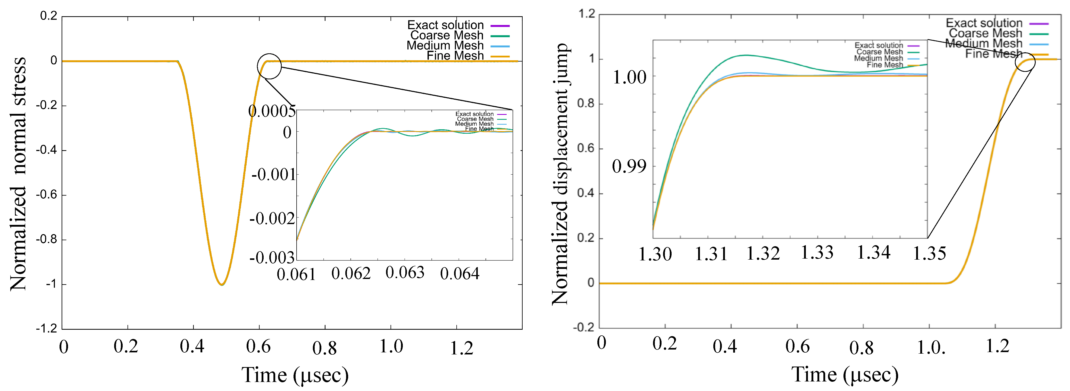
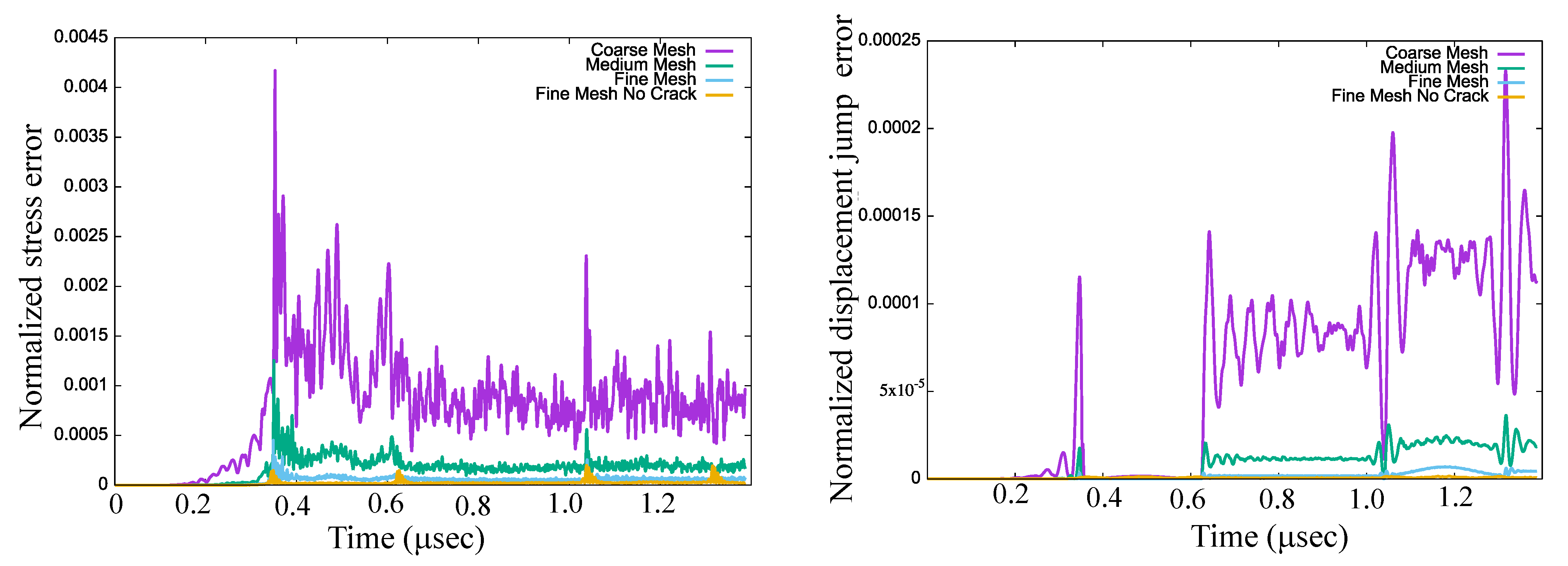
Mesh sensitivity. In Figure 2, we have plotted the time evolution of the normalized averaged stress $t\to {\overline{\sigma }}_{xx}(t)={\int }_{\Sigma }{\sigma }_{xx}(t,l,y)dy$ (left) and of the normalized averaged displacement jump $t\to [{\overline{u}}_x](t)={\int }_{\Sigma }[u_x](t,l,y)dy$ (right) in $\Sigma$ for three different meshes versus the exact solution. All the computations have been done with a fixed time step $\Delta t=T/4000$ (corresponding to a CFL of 0.0178 for the coarse mesh, 0.0379 for the medium mesh and 0.0752 for the finer mesh). We see that the compression pulse travels through the interface $\Sigma$ without any perturbation (no displacement jump), but after the reflection at $x=L$ the traction wave will generate a separation (displacement jump). We remark that the exact solution and the computed one are very close. To see the difference we have zoomed in on the end of the stress pulse during the compression phase of the interface $\Sigma$ and the beginning of the displacement jump generated by the reflected wave. We see in both zooms that the numerical solutions corresponding to the medium and fine mesh are very close to the exact one. To see that more precisely, we have plotted in Figure 3 the stress absolute error $E_{\sigma }$ (left) and the displacement jump absolute error $E_{[u]}$ (right) for the three meshes. As before, we remark that the errors of medium and fine meshes are very small. Moreover the error of the fine mesh is of the same order as the error associated with the wave propagator leapfrog-DG method (see “Fine mesh no crack” in Figure 3) without any unilateral conditions.

4.2. Frictional Slip

In the second test we wanted to see how the numerical scheme works for the frictional slip and to test the numerical approach of the stress problem. For that we have considered an elastic body $\Omega$ under a spherical compressive stress $p=A_{\sigma }$ acting on all the boundaries (${\sigma }_n=-A_{\sigma }$ on $\partial \Omega$); at $y=-b$ and $y=b$ the tangential velocity was vanishing (i.e., $v_x=0$). We also imposed a vanishing tangential stress (${\sigma }_{xy}(t,L)=0$ ) at $x=L$, and for $x=0$ we considered a loading tangential pulse $F(t)$ (i.e., ${\sigma }_{xy}(t,0)=F(t)$), with $F(t)=A_{\sigma }{\mathit{\phi }}_{\delta }(t-\delta )$). Here $A_{\sigma }>0$ is the stress amplitude and ${\mathit{\phi }}_{\delta }$ was defined in the previous subsection. At the interface $\Sigma$ we considered a Coulomb friction law ($[u_x]=0,$$[{\sigma }_{xx}]=[{\sigma }_{xy}]=0,|{\sigma }_{xy}|+{\mu }_f{\sigma }_{xx}⩽0,(|{\sigma }_{xy}|+{\mu }_f{\sigma }_{xx})[v_y]=0,{\sigma }_{xy}[v_y]⩽0$). The frictional coefficient ${\mu }_f$ was chosen to be ${\mu }_f=0.5$. At $t=0$, the elastic body was at rest (${\mathit{v}}_0=0$) and under a spherical pressure ${\sigma }_0=-A_{\sigma }\mathit{I}$.

The tangential stress condition at $x=0$ generates a shear wave which will propagate into the body, arriving at the frictional interface $\Sigma$. Since the amplitude of the shear wave $A_{\sigma }$ is larger than the frictional threshold ${\mu }_{f}p={\mu }_f{A}_{\sigma }$, the slab will start to slip and part of the pulse is transmitted on the right side, while the other part will be reflected on left side of the interface. Let us notice that the problem has an one-dimensional solution with ${\sigma }_{xx}={\sigma }_{yy}=-A_{\sigma },v_x=0,v_y=v_y(t,x),{\sigma }_{xy}={\sigma }_{xy}(t,x)$ and the problem can be reduced to a first order hyperbolic system for $v_y$ and ${\sigma }_{xy}$ with the associated speed velocity $c=c_S=\sqrt{G/\rho }$. The time interval of interest will be $[0,T]$, with $T=L/c_s$, such that the wave which starts at $x=0$ has the time to arrive at $x=l$ and capture the switches no-slip/slip and slip/no-slip. As before, we computed the exact solution on the fault $\Sigma$ using the method of characteristics. If we denote by $t^{\prime }$ and $t^{″}$ the instances when $F(t^{\prime }-l/c_s)=F(t^{″}-l/c_s)={\mu }_f{A}_{\sigma }$, with $t^{\prime }<t^{″}$, then the two slabs will slip ($[v_y](t,l)>0$) during the time interval $[t^{\prime },t^{″}]$, while in the rest of the time no slip occurs ($[v_y](t,l)=0$). The analytical solution can be computed for each time interval:

$${\sigma }_{xy}^{ex}(t,l)=F(t-\frac{l}{c}),v_y^{ex}(t,l-)=v_y^{ex}(t,l+)={\displaystyle \frac{F(t-\frac{l}{c})}{\sqrt{\rho G}}},\mathrm{for}t\in [0,t^{\prime }]\cup [t^{″},T],$$

$${\sigma }_{xy}^{ex}(t,l)={\mu }_f{A}_{\sigma },v_y^{ex}(t,l-)={\displaystyle \frac{-{\mu }_f{A}_{\sigma }}{\sqrt{\rho G}}}x,v_y^{ex}(t,l+)={\displaystyle \frac{{\mu }_f{A}_{\sigma }-2F(t-\frac{l}{c})}{\sqrt{\rho G}}},\mathrm{for}t\in [t^{\prime },t^{″}].$$

Choice of parameters. The iterative algorithm for the stress problem stops when the relative error $\parallel {\sigma }_{i+1}^{k+\frac{3}{2}}-{\sigma }_i^{k+\frac{3}{2}}{\parallel }_{{\mathcal{D}}_h^{\Sigma }}/{\parallel {\sigma }_i^{k+\frac{3}{2}}\parallel }_{{\mathcal{D}}_h^{\Sigma }}$ is less than the tolerance $T_{\sigma }$ (related to the Uzawa parameter $r_s$). The best choice we found for the numerical parameter $r_s$ in the Lagrangian approach was ${\displaystyle r_f=\frac{1}{\sqrt{G\rho }}}$. For this choice of $r_f$, the convergence was rapid at a tolerance around ${10}^{-4}$. If the tolerance is larger than ${10}^{-3}$, spurious oscillations could appear, but the algorithm is still stable. For tolerance smaller that $T_{\sigma }={10}^{-4}$, the computational time increases without any significant decrease in the error. In the following computations we have chosen $T_{\sigma }={10}^{-4}$.

Stability. As before, we numerically checked the stability of the proposed numerical scheme to see how the leapfrog DG scheme is affected by our Lagrangian approach of the frictional condition. After several tests, we found that the numerical scheme is stable for a CFL coefficient less than 0.128649 for the corse mesh, less than 0.136483 for the medium mesh and less than 0.13556 for the fine mesh. These values have to be compared with the maximum CFL coefficient found for the DG leap-frog scheme without any frictional conditions (around 0.28; see the previous subsection). We can conclude that we have to choose a time step for the frictional stability such that the CFL coefficient is less than 0.12.

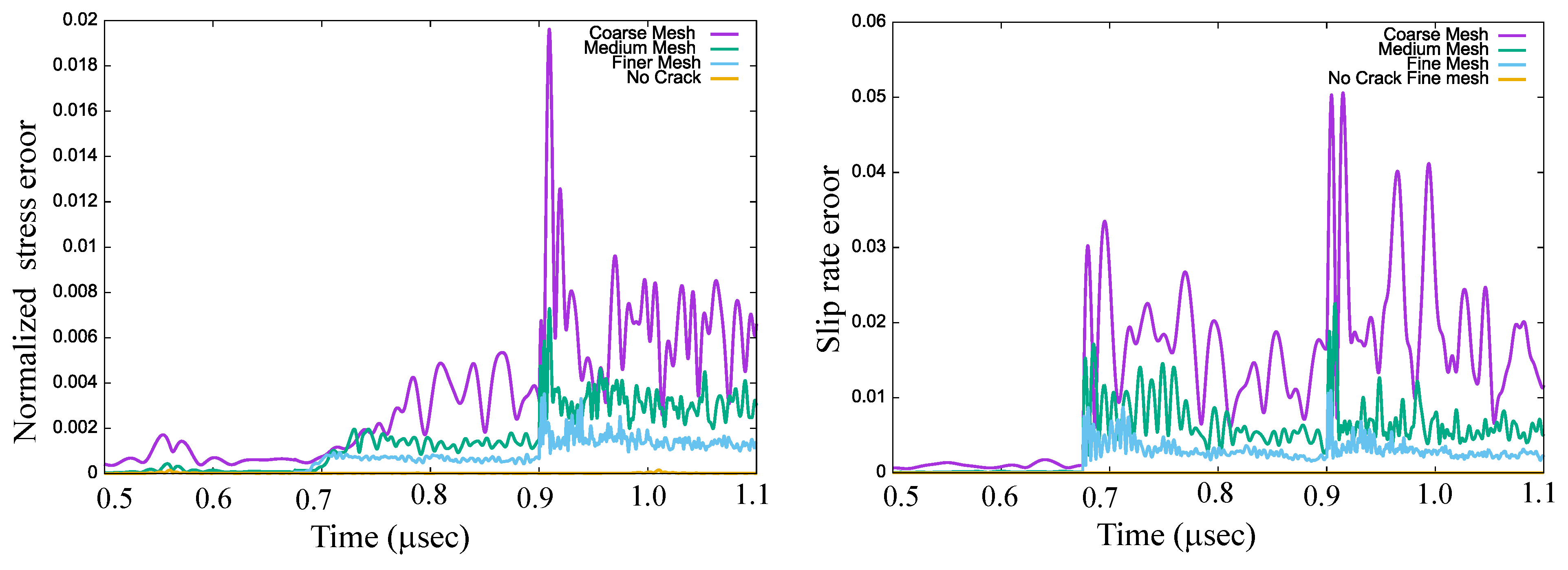
To see how the proposed numerical scheme approaches the frictional boundary condition, we have computed the absolute error of the tangential velocity jump (or slip rate) $E_{[v]}$:

$$E_{[v]}(t)=\frac{1}{A_u}\sqrt{\frac{{\int }_{\Sigma }{([v_y](t,l,y)-[v_y^{ex}](t,l))}^{2}dy}{|\Sigma |}},$$

(38)

where $A_v=A_{\sigma }/(c\rho )$ is the velocity amplitude, and the absolute error of the tangential stress $E_{\sigma }$ on the crack $\Sigma$, is given by

$$E_{\sigma }(t)=\frac{1}{A_{\sigma }}\sqrt{\frac{{\int }_{\Sigma }{({\sigma }_{xy}(t,l,y)-{\sigma }_{xy}^{ex}(t,l))}^{2}dy}{|\Sigma |}}.$$

(39)

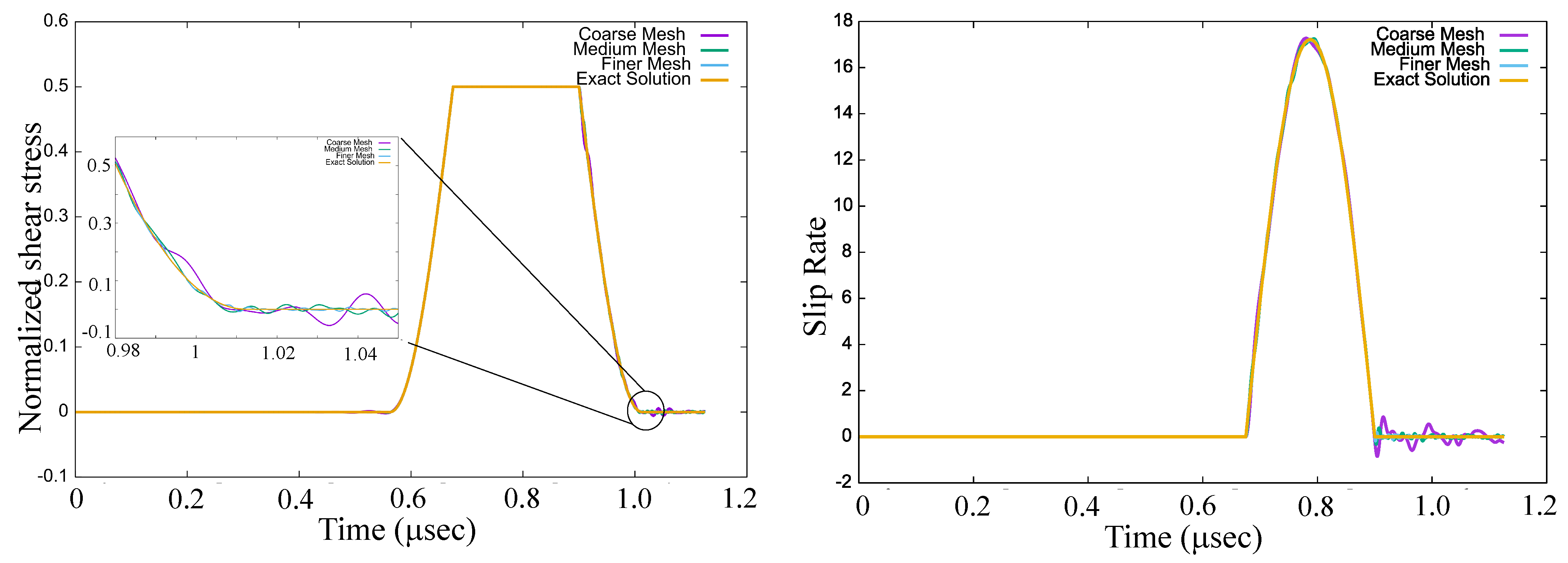
Mesh sensitivity. In Figure 4, we have plotted the time evolution of the normalized averaged stress $t\to {\overline{\sigma }}_{xy}(t)={\int }_{\Sigma }{\sigma }_{xy}(t,l,y)dy$ (left) and of the normalized averaged velocity jump $t\to [{\overline{v}}_y](t)={\int }_{\Sigma }[v_y](t,l,y)dy$ (right) in $\Sigma$ for three different meshes against the exact solution. All the computations have been done with a fixed time step $\Delta t=T/4000$ (corresponding to a CFL of 0.0289 for the coarse mesh, 0.0614 for the medium mesh and 0.122 for the finer mesh). We can observe a plateau in the loading pulse due to the activation of the friction conditions, generating a frictional slip and a wave reflection. We remark on the very good accuracy of the proposed numerical scheme (numerical and analytical solutions are superposed). To see the difference, we have zoomed in on the end of the stress pulse. As before, we can observe an improvement in the numerical solution with regard to the mesh refinement: the numerical solutions corresponding to the medium and fine meshes are very close to the exact one. Only small spurious oscillations are present at the front of the wave. To see that more precisely, we have plotted in Figure 5 the stress absolute error $E_{\sigma }$ (left) and the slip rate absolute error $E_{[v]}$ (right) for the three meshes. As before, we remark that the errors of medium and fine meshes are very small. In contrast, with the unilateral condition, discussed earlier, the error of the fine mesh is larger than the error associated with the wave propagator leapfrog-DG method (see “Fine mesh no crack” in Figure 5) without any frictional conditions.

5. Blast Impact on a Cracked Material

The aim of this section is to illustrate how the DG method introduced above can be used to investigate more complex wave propagation phenomena. Since 3D computations, involving intensive parallel computing techniques for engineering applications, are beyond the scope of this theoretical paper, we only deal with 2D computations.

5.1. Anti-Plane Blast in a Meta-Material

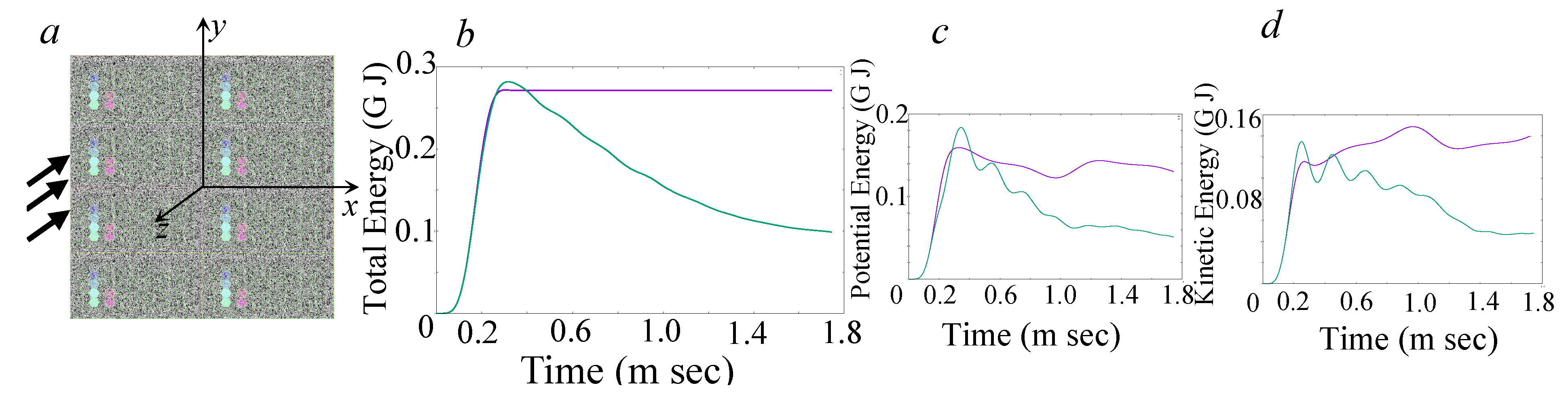
The central focus here is an architected meta-material, designed to blast energy dissipation, with a hexagonal distribution of the micro-cracks. In Figure 6a we have plotted the mesh with an 8-subdomain decomposition for parallel computing. Each subdomain contains 75 hexagonal cells separated by micro-cracks. The meta-material, which was pre-stressed with a hydro-static pressure $-p\mathit{I}$, was impacted by a blast pulse located at the center of the left side (see Figure 6a), and all the other boundaries were stress-free. For simplicity we have considered here the anti-plane configuration; hence, the two sides of all micro-cracks were always in contact.

Since the main objective was observing the energy dissipation, we have plotted in Figure 6b–d the evolution of the total, kinetic and potential energies (in red) compared with the case without cracks (in blue). We note that around 63% of the total energy was dissipated through the frictional slip in the micro-cracks.

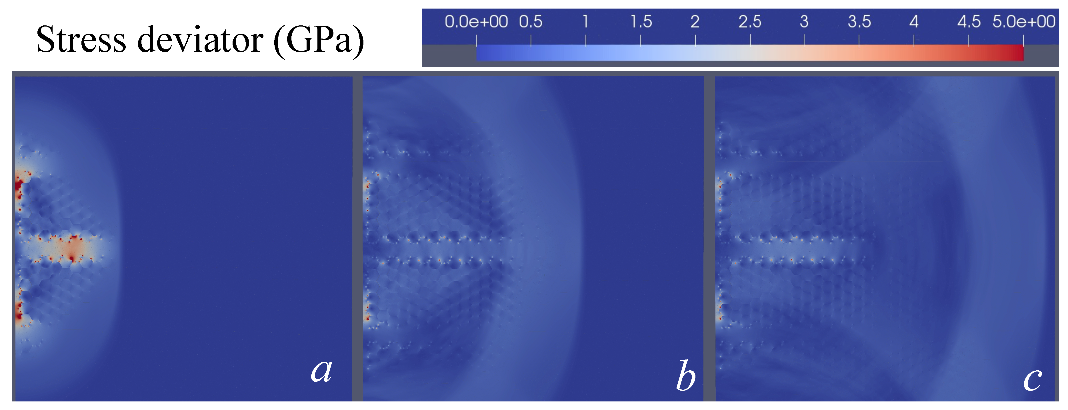
In Figure 7, we have plotted the evolution of the stress deviator during the blast propagation in the meta-material. As expected, the central part near the blast inital location was the most affected, but the blast wave succeeded in generating frictional slip in a large region. This frictional slip is associated with residual stresses.

5.2. In-Plane Blast for an Anisotropic Crack Distribution

We considered a (compressive) in-plane blast-wave propagation in a ceramic block with an anisotropic crack distribution. The elastic domain $\Omega =(0,a)\times (0,5a)$, in a plane-stress configuration, was impacted at the left side $x=0,y\in (2a,3a)$ by a compressive pulse $t\to S(t)$ with an amplitude $-A_{\sigma }$ and time duration $2\delta =0.5a/c_P$ (see Figure 8a). The faces $y=0$ and $y=5a$ were fixed, and the face $x=a$ was stress-free. The numerical computations were done over the time interval $[0,T]$ with $T=2a/c_p$ in a domain containing $M=72$ micro-cracks inclined at the angle $\theta$. The loading compressive wave was traveling into the cracked material till it reached the stress-free boundary, when it was reflected as a traction loading wave. We considered two cases corresponding to frictionless and frictional contact with the micro-cracks.

5.2.1. Frictionless Contact

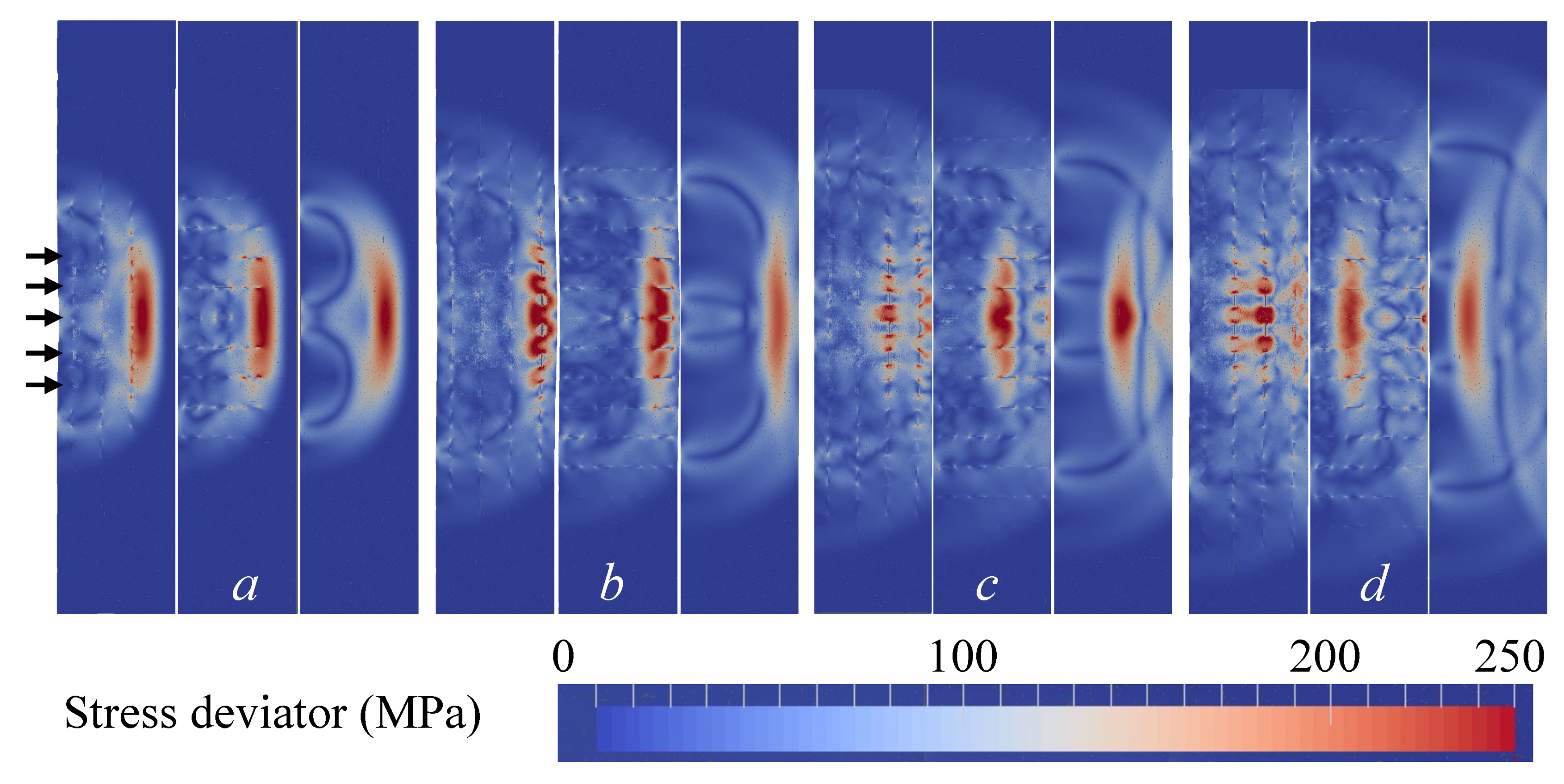
In Figure 8, we show the comparison between the propagation of a blast wave in a cracked material and an undamaged one with the stress deviator on a color scale. For the micro-cracks being vertically oriented ($\theta =\pi /2$, in Figure 8 left), we can observe at $t=0.5T$, the instance before the pulse reaches the boundary, a high concentration of the stress in the middle of the pulse which is propagating as a P-wave. The micro-cracks are not opening and the P-wave is not really affected by the presence of the micro-cracks. At the tips of the impact zone, we remark two S-waves acting in mode II. In the following frames, at $t=0.7T$ and $t=0.8T$, just after the pulse is reflected by the stress boundary, we remark that the micro-cracks are opening, generating stress concentration at the tips of the cracks, giving an irregular shape to the wave. The S-waves are perturbed, but an overall behavior can be observed. In the following frame, at $t=0.9T$, we remark that the cracks near the right boundary begin to close. In all frames, we observe that the S-waves are not too scattered.

For micro-cracks horizontally oriented ($\theta =0$), one can see in Figure 8 middle) that, at $t=0.5T$, the S-waves are almost completely scattered, but the P-wave is well represented. This is due to the fact that horizontal micro-cracks are active in the shearing process (Mode II) but almost inactive in Mode I. At $t=0.7T$, we found that the micro-cracks near the right boundary are opening, giving a high concentration of the deviatoric stress, but the P-waves are not as affected as in the vertical case. However, the overall shape of the wave is preserved. In the last two frames we remark that the loading wave is less scattered than in the previous case (vertical orientation), but in all frames we observe an important scattering of the S-waves.

If the micro-cracks are oriented $\theta =\pi /4$, we can see in Figure 9-middle that, at $t=0.5T$, due to cracks acting in mode II, the P-Wave is already perturbed. After the reflection ($t=0.7T$), we can observe that more rightward cracks begin to open. In the last two frames the cracks are active in mode I and II, and it is difficult to distinguish an overall behavior of the resulting scattered wave.

5.2.2. Frictional Contact

We analyze here the role played by the friction, acting on the micro-cracks’ sides, in the wave propagation. Globally, we expected that the friction has a stabilization effect and the waves are less perturbed by the presence of the micro-cracks. This is due to the fact that cracks have more resistance to slip in mode II. On the contrary, mode I activation of the micro-cracks is not affected by the friction. The friction coefficient was chosen to be ${\mu }_f=0.5$.

We have plotted in Figure 10 the evolution of the stress deviator during the reflection of the blast wave on the free stress boundary for a material with vertical frictional micro-cracks. We remark that, due to friction, the incident S-wave does not open the cracks (working in the mode II). For the reflected wave, when the cracks work mainly in mode I, the friction has a negligible influence on the wave propagation.

In Figure 9 we show several frames of blast propagation in a cracked material with friction, without friction and in an undamaged one (with the stress deviator in the color scale) for micro-cracks oriented $\theta =\pi /4$. The first snapshot is at $t=0.5T$ (a), and we note the loss of symmetry in the horizontal plane. In the frictional case, the waves (P and S) are less scattered than in the frictionless case. Indeed, all the micro-cracks are working in mode II at this stage, where friction implies a “damage decrease”. For $t=0.7T$ (b), when the reflected wave is in traction, we remark that in both cases the cracks next to the right boundary start to open, working in mode I. However, the P-wave has a larger amplitude in the frictional case than in the other one. The other cracks are working in mode II, and as before, we remark that the S-waves are more scattered in the frictionless case. In the last two frames (c,d), we observe that in both cases the waves are spread out and it is difficult to distinguish between the frictional and frictionless propagation. This is due to the key role played by the mode I activation of the micro-cracks in damage evolution, which affects the waves’ propagation.

6. Conclusions

The qualitative and quantitative investigation of the wave propagation in (damaged) materials with a nonlinear micro-structure (micro-cracks in frictional contact) needs robust, efficient and accurate numerical schemes. This paper proposes a new method based on the interplay between the leapfrog scheme (for the time discretization) and the augmented Lagrangian algorithm (to solve the associated non-linear problems). For an efficient parallelization of the computations, a DG method was used for the space discretization. Since the Lagrangian algorithm concerns only the degrees of freedom associated with the interfaces, the additional computational effort is small with respect to that needed for the wave propagation in the same domain without any interfaces.

This numerical method was tested through two model problems for which other analytical solutions exist. In both cases we analyzed the stability and the mesh sensitivity. To illustrate the numerical scheme, the wave generated by a blast in a cracked material with multiple interfaces has been analyzed.

Future developments of this work could include 3D computations for engineering applications, involving intensive parallel computing techniques, to investigate the wave propagation in elastic solids with micro-cracks (cracked solid) for a better understanding of dynamic damage in brittle materials or in architected meta-materials.

References

- Mavko, G.; Mukerji, T.; Dvorkin, J. The Rock Physics Handbook: Tools for Seismic Analysis of Porous Media; Cambridge University Press: Cambridge, UK, 2009. [Google Scholar]
- Hudson, J.; Pointer, T.; Liu, E. Effective-medium theories for fluid-saturated materials with aligned cracks. Geophys. Prospect. 2001, 49, 509–522. [Google Scholar] [CrossRef] [Green Version]
- Schoenberg, M.; Sayers, C.M. Seismic anisotropy of fractured rock. Geophysics 1995, 60, 204–211. [Google Scholar] [CrossRef]
- Thomsen, L. Elastic anisotropy due to aligned cracks in porous rock. Geophys. Prospect. 1995, 43, 805–829. [Google Scholar] [CrossRef]
- Schubnel, A.; Guéguen, Y. Dispersion and anisotropy of elastic waves in cracked rocks. J. Geophys. Res. Solid Earth 2003, 108. [Google Scholar] [CrossRef] [Green Version]
- Malik, I.; Mirkhalaf, M.; Barthelat, F. Bio-inspired “jigsaw”-like interlocking sutures: Modeling, optimization, 3D printing and testing. J. Mech. Phys. Solids 2017, 102, 224–238. [Google Scholar] [CrossRef]
- van Baren, G.B.; Mulder, W.A.; Herman, G.C. Finite-difference modeling of scalar-wave propagation in cracked media. Geophysics 2001, 66, 267–276. [Google Scholar] [CrossRef]
- Saenger, E.H.; Shapiro, S.A. Effective velocities in fractured media: A numerical study using the rotated staggered finite-difference grid. Geophys. Prospect. 2002, 50, 183–194. [Google Scholar] [CrossRef]
- Saenger, E.H.; Krüger, O.S.; Shapiro, S.A. Effective elastic properties of randomly fractured soils: 3D numerical experiments. Geophys. Prospect. 2004, 52, 183–195. [Google Scholar] [CrossRef]
- Virieux, J. P-SV wave propagation in heterogeneous media: Velocity-stress finite-difference method. Geophysics 1986, 51, 889–901. [Google Scholar] [CrossRef]
- Saenger, E.H.; Gold, N.; Shapiro, S.A. Modeling the propagation of elastic waves using a modified finite-difference grid. Wave Motion 2000, 31, 77–92. [Google Scholar] [CrossRef]
- Schoenberg, M. Elastic wave behavior across linear slip interfaces. J. Acoust. Soc. Am. 1980, 68, 1516–1521. [Google Scholar] [CrossRef] [Green Version]
- Vlastos, S.; Liu, E.; Main, I.; Li, X.Y. Numerical simulation of wave propagation in media with discrete distributions of fractures: Effects of fracture sizes and spatial distributions. Geophys. J. Int. 2003, 152, 649–668. [Google Scholar] [CrossRef] [Green Version]
- Zhang, J. Elastic wave modeling in fractured media with an explicit approach. Geophysics 2005, 70, T75–T85. [Google Scholar] [CrossRef]
- Martins, J.; Oden, J. A numerical analysis of a class of problems in elastodynamics with friction. Comput. Methods Appl. Mech. Eng. 1983, 40, 327–360. [Google Scholar] [CrossRef]
- Oden, J.; Martins, J. Models and computational methods for dynamic friction phenomena. Comput. Methods Appl. Mech. Eng. 1985, 52, 527–634. [Google Scholar] [CrossRef]
- Arnold, D.N.; Brezzi, F.; Cockburn, B.; Marini, L.D. Unified analysis of discontinuous Galerkin methods for elliptic problems. SIAM J. Numer. Anal. 2002, 39, 1749–1779. [Google Scholar] [CrossRef]
- Simo, J.C.; Laursen, T. An augmented Lagrangian treatment of contact problems involving friction. Comput. Struct. 1992, 42, 97–116. [Google Scholar] [CrossRef]
- Pietrzak, G.; Curnier, A. Large deformation frictional contact mechanics: Continuum formulation and augmented Lagrangian treatment. Comput. Methods Appl. Mech. Eng. 1999, 177, 351–381. [Google Scholar] [CrossRef]
- Zavarise, G.; Wriggers, P.; Schrefler, B. A method for solving contact problems. Int. J. Numer. Methods Eng. 1998, 42, 473–498. [Google Scholar] [CrossRef]
- McDevitt, T.; Laursen, T. A mortar-finite element formulation for frictional contact problems. Int. J. Numer. Methods Eng. 2000, 48, 1525–1547. [Google Scholar] [CrossRef]
- El-Abbasi, N.; Bathe, K.J. Stability and patch test performance of contact discretizations and a new solution algorithm. Comput. Struct. 2001, 79, 1473–1486. [Google Scholar] [CrossRef] [Green Version]
- Wriggers, P. Finite element algorithms for contact problems. Arch. Comput. Methods Eng. 1995, 2, 1–49. [Google Scholar] [CrossRef]
- Belgacem, F.B. The mortar finite element method with Lagrange multipliers. Numer. Math. 1999, 84, 173–197. [Google Scholar] [CrossRef]
- Belgacem, F.B.; Hild, P.; Laborde, P. Extension of the mortar finite element method to a variational inequality modeling unilateral contact. Math. Model. Methods Appl. Sci. 1999, 9, 287–303. [Google Scholar] [CrossRef]
- Laursen, T.A.; Puso, M.A.; Sanders, J. Mortar contact formulations for deformable–deformable contact: Past contributions and new extensions for enriched and embedded interface formulations. Comput. Methods Appl. Mech. Eng. 2012, 205, 3–15. [Google Scholar] [CrossRef]
- Temizer, I. A mixed formulation of mortar-based contact with friction. Comput. Methods Appl. Mech. Eng. 2013, 255, 183–195. [Google Scholar] [CrossRef]
- Popp, A.; Wall, W. Dual mortar methods for computational contact mechanics–overview and recent developments. GAMM-Mitteilungen 2014, 37, 66–84. [Google Scholar] [CrossRef]
- Sitzmann, S.; Willner, K.; Wohlmuth, B.I. A dual Lagrange method for contact problems with regularized frictional contact conditions: Modelling micro slip. Comput. Methods Appl. Mech. Eng. 2015, 285, 468–487. [Google Scholar] [CrossRef]
- Masud, A.; Truster, T.J.; Bergman, L.A. A unified formulation for interface coupling and frictional contact modeling with embedded error estimation. Int. J. Numer. Methods Eng. 2012, 92, 141–177. [Google Scholar] [CrossRef]
- Wriggers, P.; Zavarise, G. A formulation for frictionless contact problems using a weak form introduced by Nitsche. Comput. Mech. 2008, 41, 407–420. [Google Scholar] [CrossRef]
- Annavarapu, C.; Hautefeuille, M.; Dolbow, J.E. A Nitsche stabilized finite element method for frictional sliding on embedded interfaces. Part I: Single interface. Comput. Methods Appl. Mech. Eng. 2014, 268, 417–436. [Google Scholar] [CrossRef]
- Truster, T.J.; Masud, A. Primal interface formulation for coupling multiple PDEs: A consistent derivation via the variational multiscale method. Comput. Methods Appl. Mech. Eng. 2014, 268, 194–224. [Google Scholar] [CrossRef]
- Annavarapu, C.; Hautefeuille, M.; Dolbow, J.E. Stable imposition of stiff constraints in explicit dynamics for embedded finite element methods. Int. J. Numer. Methods Eng. 2012, 92, 206–228. [Google Scholar] [CrossRef]
- Arnold, D.N. An interior penalty finite element method with discontinuous elements. SIAM J. Numer. Anal. 1982, 19, 742–760. [Google Scholar] [CrossRef]
- Hansbo, P.; Larson, M.G. Discontinuous Galerkin methods for incompressible and nearly incompressible elasticity by Nitsche’s method. Comput. Methods Appl. Mech. Eng. 2002, 191, 1895–1908. [Google Scholar] [CrossRef]
- Lew, A.; Neff, P.; Sulsky, D.; Ortiz, M. Optimal BV estimates for a discontinuous Galerkin method for linear elasticity. Appl. Math. Res. Express 2004, 2004, 73–106. [Google Scholar] [CrossRef]
- Ten Eyck, A.; Lew, A. Discontinuous Galerkin methods for non-linear elasticity. Int. J. Numer. Methods Eng. 2006, 67, 1204–1243. [Google Scholar] [CrossRef]
- Truster, T.J.; Chen, P.; Masud, A. On the algorithmic and implementational aspects of a Discontinuous Galerkin method at finite strains. Comput. Math. Appl. 2015, 70, 1266–1289. [Google Scholar] [CrossRef]
- Noels, L.; Radovitzky, R. A general discontinuous Galerkin method for finite hyperelasticity. Formulation and numerical applications. Int. J. Numer. Methods Eng. 2006, 68, 64–97. [Google Scholar] [CrossRef]
- Nguyen, V.D.; Becker, G.; Noels, L. Multiscale computational homogenization methods with a gradient enhanced scheme based on the discontinuous Galerkin formulation. Comput. Methods Appl. Mech. Eng. 2013, 260, 63–77. [Google Scholar] [CrossRef] [Green Version]
- Truster, T.J.; Masud, A. Discontinuous Galerkin Method for Frictional Interface Dynamics. J. Eng. Mech. 2016, 142, 04016084. [Google Scholar] [CrossRef] [Green Version]
- Truster, T.J.; Masud, A. A discontinuous/continuous Galerkin method for modeling of interphase damage in fibrous composite systems. Comput. Mech. 2013, 52, 499–514. [Google Scholar] [CrossRef]
- Abedi, R.; Haber, R.; Thite, S.; Erickson, J. An h-adaptive spacetime-discontinuous Galerkin method for linearized elastodynamics. Eur. J. Comput. Mech. 2006, 6, 619–642. [Google Scholar] [CrossRef] [Green Version]
- Miller, S.; Kraczek, B.; Haber, R.; Johnson, D. Multi-field space time discontinuous Galerkin methods for linearized elastodynamics. Comput. Methods Appl. Mech. Eng. 2009, 199, 34–47. [Google Scholar] [CrossRef]
- Abedi, R.; Hawker, M.; Haber, R.; Matous, K. An adaptive spacetime discontinuous Galerkin method for cohesive models of elastodynamic fracture. Int. J. Numer. Methods Eng. 2009, 81, 1–42. [Google Scholar] [CrossRef]
- Etienne, V.; Chaljub, E.; Virieux, J.; Glinsky, N. An hp-adaptive discontinuous Galerkin finite-element method for 3-D elastic wave modelling. Geophys. J. Int. 2010, 183, 941–962. [Google Scholar] [CrossRef] [Green Version]
- Abedi, R.; Haber, R. Riemann solutions and spacetime dis- continuous Galerkin method for linear elastodynamic contact. Comput. Methods Appl. Mech. Eng. 2014, 270, 150–177. [Google Scholar] [CrossRef]
- Gomez, Q.; Ciobanu, O.; Ionescu, I. Numerical modeling of wave propagation in a cracked solid. Math. Mech. Solids 2019, 24, 2895–2913. [Google Scholar] [CrossRef]
- Benjemaa, M.; Glinsky-Olivier, N.; Cruz-Atienza, V.M.; Virieux, J. 3-D dynamic rupture simulations by a finite volume method. Geophys. J. Int. 2009, 178, 541–560. [Google Scholar] [CrossRef] [Green Version]
- Delcourte, S.; Fezoui, L.; Glinsky-Olivier, N. A high-order discontinuous Galerkin method for the seismic wave propagation. ESAIM Proc. 2009, 27, 70–89. [Google Scholar] [CrossRef] [Green Version]
- Kaser, M.H.V.; de la Puente, J. Quantitative accuracy analysis of the discontinuous Galerkin method for seismic wave propagation. Geophys. J. Int. 2008, 173, 990–999. [Google Scholar] [CrossRef] [Green Version]
Figure 1.
Representation of the elastic domain and of its boundary : the external one, where the velocity () and the stress vector () are imposed, and the internal one () with frictional micro-cracks.
Figure 2.
The time evolution of the normalized averaged stress (left) and of the normalized averaged displacement jump (right) in for three different meshes, and the exact solution. Zoom of the wave front.
Figure 3.
The time evolution of the stress absolute error (left) and of the displacement jump absolute error (right) for three different meshes. To be compared with the associated error of the DG method without any unilateral condition on computed with the fine mesh.
Figure 4.
The time evolution of the normalized averaged stress (left) and of the averaged slip rate (right) in for three different meshes and the exact solution. Zoom of the wave front.
Figure 5.
The time evolution of the stress absolute error (left) and of the slip rate absolute error (right) for three different meshes. To be compared with the associated error of the DG method without any unilateral condition on computed with the fine mesh.
Figure 6.
Blast in an architected meta-material with internal micro-cracks in the anti-plane configuration. The mesh with a distribution of hexagonal cells with an 8-subdomains decomposition (a). The evolution of the total (b), kinetic (c) and potential (d) energies with frictional slip (red) and without damage (no cracks or no slip in blue).
Figure 7.
Anti-plane blast propagation in an architected meta-material. Three snapshots of the stress deviator (color scale in GPa) at (a), (b) and and (c).
Figure 8.
Role of the micro-cracks orientation in wave propagation for frictionless contact. Four snapshots of the stress deviator (color scale in MPa) for vertical (left) and horizontal (middle) micro-cracks and an undamaged material (no-cracks, (right)) at (a), (b), (c) and (d).
Figure 9.
Role of friction in wave propagation for micro-cracks oriented . Four snapshots of the stress deviator (color scale in MPa) for frictional (left) and frictionless (middle) contact and undamaged material (no-cracks, (right)) at (a), (b), (c) and (d).
Figure 10.
Blast propagation for frictional vertical micro-cracks. (Left) Four snapshots of the stress deviator (color scale in MPa) at (a), (b), (c) and (d). (Right) Zoom of the central part.
Publisher’s Note: MDPI stays neutral with regard to jurisdictional claims in published maps and institutional affiliations. |
© 2022 by the authors. Licensee MDPI, Basel, Switzerland. This article is an open access article distributed under the terms and conditions of the Creative Commons Attribution (CC BY) license (https://creativecommons.org/licenses/by/4.0/).
Share and Cite
MDPI and ACS Style
Gomez, Q.; Goument, B.; Ionescu, I.R. A Lagrangian DG-Method for Wave Propagation in a Cracked Solid with Frictional Contact Interfaces. Mathematics 2022, 10, 871. https://0-doi-org.brum.beds.ac.uk/10.3390/math10060871
AMA Style
Gomez Q, Goument B, Ionescu IR. A Lagrangian DG-Method for Wave Propagation in a Cracked Solid with Frictional Contact Interfaces. Mathematics. 2022; 10(6):871. https://0-doi-org.brum.beds.ac.uk/10.3390/math10060871
Chicago/Turabian StyleGomez, Quriaky, Benjamin Goument, and Ioan R. Ionescu. 2022. "A Lagrangian DG-Method for Wave Propagation in a Cracked Solid with Frictional Contact Interfaces" Mathematics 10, no. 6: 871. https://0-doi-org.brum.beds.ac.uk/10.3390/math10060871
Note that from the first issue of 2016, this journal uses article numbers instead of page numbers. See further details here.