
Central Nervous System: Overall Considerations Based on Hardware Realization of Digital Spiking Silicon Neurons (DSSNs) and Synaptic Coupling

 , , , and
Abstract
:1. Introduction
2. Background
- : Bias constant;
- : Applied current for neurons;
- and : Time constant;
- and ( and ): Constants that control the nullclines of the variables (Dynamics of the model).
3. Proposed Procedure
4. Dynamic Behaviors and Time Domain Analysis
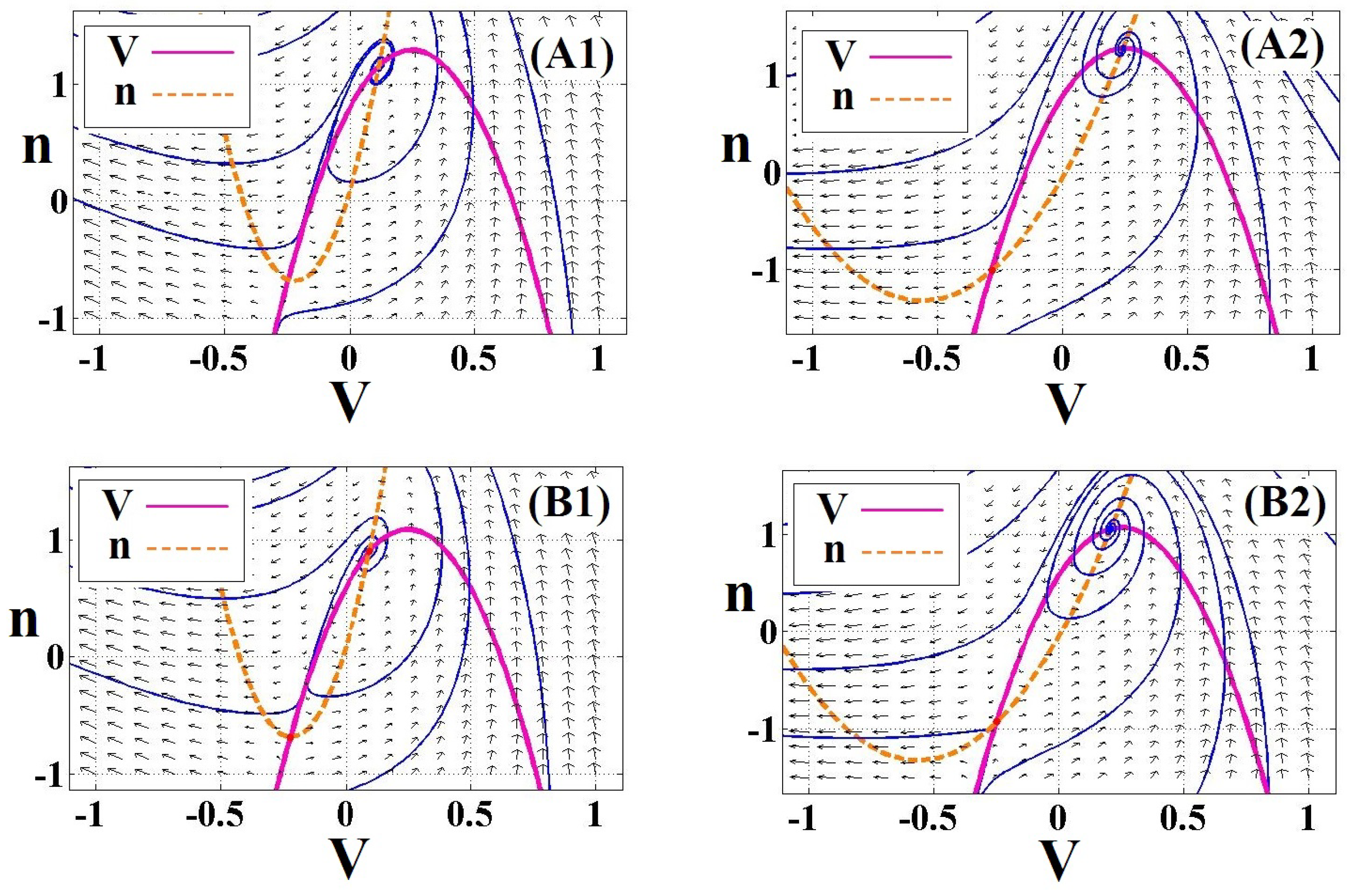
4.1. Dynamics
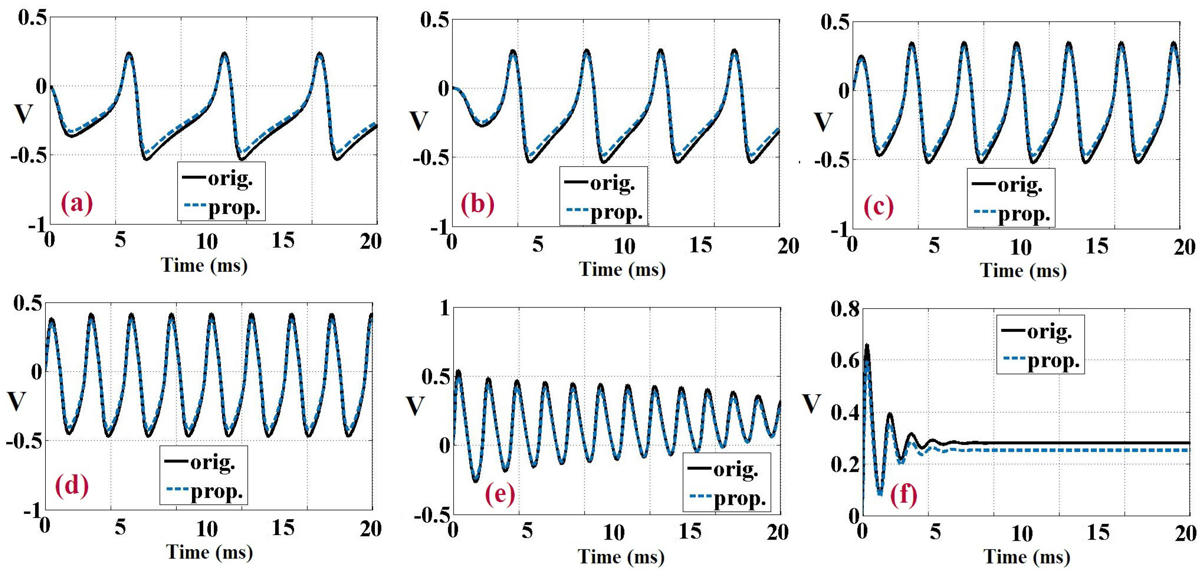
4.2. Time Domain
5. Synaptic Coupling
- : Time delay (s);
- : Responsible for the activation and relaxation of Z;
- : Relaxing the parameter Z;
- : Threshold parameter for the activation of Z;
- : Conductivity parameter;
- : Reference level of Z.
6. Overall Hardware Implementation
6.1. Scheduling Diagrams
6.2. Bit-Width Definition
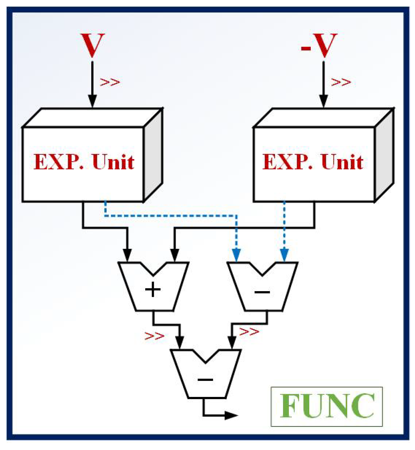
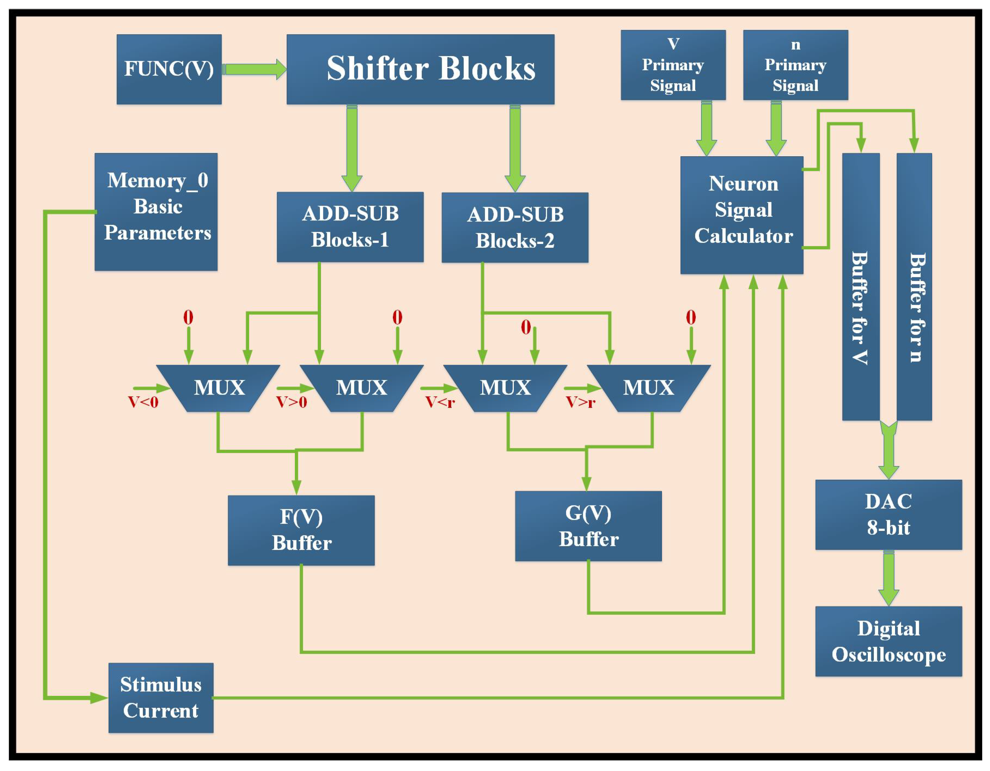
6.3. Architecture Design
7. Production Results
8. Discussion
9. Conclusions
Author Contributions
Funding
Institutional Review Board Statement
Informed Consent Statement
Data Availability Statement
Acknowledgments
Conflicts of Interest
References
- Roshani, G.H.; Feghhi, S.A.H.; Mahmoudi-Aznaveh, A.; Nazemi, E.; Adineh-Vand, A. Precise volume fraction prediction in oil–water–gas multiphase flows by means of gamma-ray attenuation and artificial neural networks using one detector. Measurement 2014, 51, 34–41. [Google Scholar] [CrossRef]
- Nazemi, E.; Feghhi, S.; Roshani, G.; Setayeshi, S.A.; Peyvandi, R.G. A radiation-based hydrocarbon two-phase flow meter for estimating of phase fraction independent of liquid phase density in stratified regime. Flow Meas. Instrum. 2015, 46, 25–32. [Google Scholar] [CrossRef]
- Roshani, G.H.; Nazemi, E.; Feghhi, S.A.; Setayeshi, S. Flow regime identification and void fraction prediction in two-phase flows based on gamma ray attenuation. Measurement 2015, 62, 25–32. [Google Scholar] [CrossRef]
- Roshani, G.H.; Nazemi, E.; Feghhi, S.A.H. Investigation of using 60Co source and one detector for determining the flow regime and void fraction in gas–liquid two-phase flows. Flow Meas. Instrum. 2016, 50, 73–79. [Google Scholar] [CrossRef]
- Nazemi, E.; Feghhi, S.; Roshani, G.; Peyvandi, R.G.; Setayeshi, S. Precise void fraction measurement in two-phase flows independent of the flow regime using gamma-ray attenuation. Nucl. Eng. Technol. 2016, 48, 64–71. [Google Scholar] [CrossRef] [Green Version]
- Roshani, G.H.; Nazemi, E.; Roshani, M.M. Flow regime independent volume fraction estimation in three-phase flows using dual-energy broad beam technique and artificial neural network. Neural Comput. Appl. 2016, 28, 1265–1274. [Google Scholar] [CrossRef]
- Nazemi, E.; Roshani, G.H.; Feghhi, S.A.H.; Setayeshi, S.; Eftekhari Zadeh, E.; Fatehi, A. Optimization of a method for identifying the flow regime and measuring void fraction in a broad beam gamma-ray attenuation technique. Int. J. Hydrogen Energy 2016, 41, 7438–7444. [Google Scholar] [CrossRef]
- Alanazi, A.K.; Alizadeh, S.M.; Nurgalieva, K.S.; Guerrero, J.W.G.; Abo-Dief, H.M.; Eftekhari-Zadeh, E.; Narozhnyy, I.M. Optimization of x-ray tube voltage to improve the precision of two phase flow meters used in petroleum industry. Sustainability 2021, 13, 3622. [Google Scholar] [CrossRef]
- Roshani, G.; Nazemi, E.; Roshani, M. Usage of two transmitted detectors with optimized orientation in order to three phase flow metering. Measurement 2017, 100, 122–130. [Google Scholar] [CrossRef]
- Roshani, G.; Nazemi, E. Intelligent densitometry of petroleum products in stratified regime of two phase flows using gamma ray and neural network. Flow Meas. Instrum. 2017, 58, 6–11. [Google Scholar] [CrossRef]
- Roshani, G.; Nazemi, E.; Roshani, M. Intelligent recognition of gas-oil-water three-phase flow regime and determination of volume fraction using radial basis function. Flow Meas. Instrum. 2017, 54, 39–45. [Google Scholar] [CrossRef]
- Roshani, G.; Nazemi, E.; Roshani, M. Identification of flow regime and estimation of volume fraction independent of liquid phase density in gas-liquid two-phase flow. Prog. Nucl. Energy 2017, 98, 29–37. [Google Scholar] [CrossRef]
- Karami, A.; Roshani, G.H.; Nazemi, E.; Roshani, S. Enhancing the performance of a dual-energy gamma ray based three-phase flow meter with the help of grey wolf optimization algorithm. Flow Meas. Instrum. 2018, 64, 164–172. [Google Scholar] [CrossRef]
- Roshani, G.H.; Roshani, S.; Nazemi, E.; Roshani, S. Online measuring density of oil products in annular regime of gas-liquid two phase flows. Measurement 2018, 129, 296–301. [Google Scholar] [CrossRef]
- Roshani, G.; Hanus, R.; Khazaei, A.; Zych, M.; Nazemi, E.; Mosorov, V. Density and velocity determination for single-phase flow based on radiotracer technique and neural networks. Flow Meas. Instrum. 2018, 61, 9–14. [Google Scholar] [CrossRef]
- Khaibullina, K.S.; Sagirova, L.R.; Sandyga, M.S. Substantiation and selection of an inhibitor for preventing the formation of asphalt-resin-paraffin deposits. Period. Tche Quim. 2020, 17, 541–551. [Google Scholar] [CrossRef]
- Karami, A.; Roshani, G.H.; Khazaei, A.; Nazemi, E.; Fallahi, M. Investigation of different sources in order to optimize the nuclear metering system of gas-oil-water annular flows. Neural Comput. Appl. 2020, 32, 3619–3631. [Google Scholar] [CrossRef]
- Roshani, M.; Sattari, M.A.; Muhammad Ali, P.J.; Roshani, G.H.; Nazemi, B.; Corniani, E.; Nazemi, E. Application of GMDH neural network technique to improve measuring precision of a simplified photon attenuation based two-phase flowmeter. Flow Meas. Instrum. 2020, 75, 101804. [Google Scholar] [CrossRef]
- Pirasteh, A.; Roshani, S.; Roshani, S. A modified class-F power amplifier with miniaturized harmonic control circuit. AEU-Int. J. Electron. Commun. 2018, 97, 202–209. [Google Scholar] [CrossRef]
- Roshani, S.; Roshani, S. Design of a very compact and sharp bandpass diplexer with bended lines for GSM and LTE applications. AEU-Int. J. Electron. Commun. 2019, 99, 354–360. [Google Scholar] [CrossRef]
- Pirasteh, A.; Roshani, S.; Roshani, S. Compact microstrip lowpass filter with ultrasharp response using a square-loaded modified T-shaped resonator. Turk. J. Electr. Eng. Comput. Sci. 2018, 26, 1736–1746. [Google Scholar] [CrossRef]
- Jamshidi, M.B.; Roshani, S.; Talla, J.; Roshani, S.; Peroutka, Z. Size reduction and performance improvement of a microstrip Wilkinson power divider using a hybrid design technique. Sci. Rep. 2021, 11, 7773. [Google Scholar] [CrossRef] [PubMed]
- Roshani, S.; Roshani, S. Design of a high efficiency class-F power amplifier with large signal and small signal measurements. Measurement 2020, 149, 106991. [Google Scholar] [CrossRef]
- Roshani, S.; Roshani, S.; Zarinitabar, A. A modified Wilkinson power divider with ultra harmonic suppression using open stubs and lowpass filters. Analog. Integr. Circuits Signal Process. 2019, 98, 395–399. [Google Scholar] [CrossRef]
- Jamshidi, M.; Siahkamari, H.; Roshani, S.; Roshani, S. A compact Gysel power divider design using U-shaped and T-shaped resonators with harmonics suppression. Electromagnetics 2019, 39, 491–504. [Google Scholar] [CrossRef]
- Roshani, S.; Jamshidi, M.B.; Mohebi, F.; Roshani, S. Design and modeling of a compact power divider with squared resonators using artificial intelligence. Wirel. Pers. Commun. 2021, 117, 2085–2096. [Google Scholar] [CrossRef]
- Chuang, M.-L. Dual-Band Impedance Transformer Using Two-Section Shunt Stubs. IEEE Trans. Microw. Theory Tech. 2010, 58, 1257–1263. [Google Scholar] [CrossRef]
- Roshani, S.; Roshani, S. A compact coupler design using meandered line compact microstrip resonant cell (MLCMRC) and bended lines. Wirel. Netw. 2021, 27, 677–684. [Google Scholar] [CrossRef]
- Lalbakhsh, A.; Mohamadpour, G.; Roshani, S.; Ami, M.; Roshani, S.; Sayem, A.S.; Alibakhshikenari, M.; Koziel, S. Design of a compact planar transmission line for miniaturized rat-race coupler with harmonics suppression. IEEE Access 2021, 9, 129207–129217. [Google Scholar] [CrossRef]
- Lalbakhsh, A.; Afzal, M.U.; Esselle, K.P.; Manda, K. All-Metal Wideband Frequency-Selective Surface Bandpass Filter for TE and TM polarizations. IEEE Trans. Antennas Propag. 2022. [Google Scholar] [CrossRef]
- Lalbakhsh, A.; Afzal, M.U.; Hayat, T.; Esselle, K.P.; Manda, K. All-metal wideband metasurface for near-field transformation of medium-to-high gain electromagnetic sources. Sci. Rep. 2021, 11, 9421. [Google Scholar] [CrossRef]
- Lalbakhsh, A.; Alizadeh, S.M.; Ghaderi, A.; Golestanifar, A.; Mohamadzade, B.; Jamshidi, M.B.; Mandal, K.; Mohyuddin, W. A Design of a Dual-Band Bandpass Filter Based on Modal Analysis for Modern Communication Systems. Electronics 2020, 9, 1770. [Google Scholar] [CrossRef]
- Lalbakhsh, A.; Jamshidi, M.B.; Siahkamari, H.; Ghaderi, A.; Golestanifar, A.; Linhart, R.; Talla, J.; Simorangkir, R.B.; Mandal, K. A Compact Lowpass Filter for Satellite Communication Systems Based on Transfer Function Analysis. AEU-Int. J. Electron. Commun. 2020, 124, 153318. [Google Scholar] [CrossRef]
- Lalbakhsh, A.; Ghaderi, A.; Mohyuddin, W.; Simorangkir, R.B.V.B.; Bayat-Makou, N.; Ahmad, M.S.; Lee, G.H.; Kim, K.W. A Compact C-Band Bandpass Filter with an Adjustable Dual-Band Suitable for Satellite Communication Systems. Electronics 2020, 9, 1088. [Google Scholar] [CrossRef]
- Alanazi, A.K.; Alizadeh, S.M.; Nurgalieva, K.S.; Nesic, S.; Grimaldo Guerrero, J.W.; Abo-Dief, H.M.; Eftekhari-Zadeh, E.; Nazemi, E.; Narozhnyy, I.M. Application of Neural Network and Time-Domain Feature Extraction Techniques for Determining Volumetric Percentages and the Type of Two Phase Flow Regimes Independent of Scale Layer Thickness. Appl. Sci. 2022, 12, 1336. [Google Scholar] [CrossRef]
- Lalbakhsh, A.; Afzal, M.U.; Esselle, K. Simulation-driven particle swarm optimization of spatial phase shifters. In Proceedings of the18th IEEE international Conference on Electromagnetics in Advanced Applications (ICEAA), Cairns, Australia, 19–23 September 2016; pp. 428–430. [Google Scholar] [CrossRef]
- Lalbakhsh, A.; Afzal, M.U.; Esselle, K.P.; Smith, S.L. Low-Cost Non-Uniform Metallic Lattice for Rectifying Aperture Near-Field of Electromagnetic Bandgap Resonator Antennas. IEEE Trans. Antennas Propag. 2020, 68, 3328–3335. [Google Scholar] [CrossRef]
- Paul, G.S.; Mandal, K.; Lalbakhsh, A. Single-layer ultra-wide stop-band frequency selective surface using interconnected square rings. AEU-Int. J. Electron. Commun. 2021, 132, 153630. [Google Scholar] [CrossRef]
- Lalbakhsh, A.; Lotfi-Neyestanak, A.A.; Naser-Moghaddasi, M. Microstrip Hairpin Bandpass Filter Using Modified Minkowski Fractal-for Suppression of Second Harmonic. IEICE. Trans. Electron. 2012, E95-C, 378–381. [Google Scholar] [CrossRef]
- Khaibullina, K.S.; Korobov, G.Y.; Lekomtsev, A.V. Development of an asphalt-resin-paraffin deposits inhibitor and substantiation of the technological parameters of its injection into the bottom-hole formation zone. Period. Tche Quim. 2020, 17, 769–781. [Google Scholar] [CrossRef]
- Roshani, M.; Phan, G.; Faraj, R.H.; Phan, N.H.; Roshani, G.H.; Nazemi, B.; Corniani, E.; Nazemi, E. Proposing a gamma radiation based intelligent system for simultaneous analyzing and detecting type and amount of petroleum by-products. Neural Eng. Technol. 2021, 53, 1277–1283. [Google Scholar] [CrossRef]
- Roshani, M.; Phan, G.T.; Ali, P.J.M.; Roshani, G.H.; Hanus, R.; Duong, T.; Corniani, E.; Nazemi, E.; Kalmoun, E.M. Evaluation of flow pattern recognition and void fraction measurement in two phase flow independent of oil pipeline’s scale layer thickness. Alex. Eng. J. 2021, 60, 1955–1966. [Google Scholar] [CrossRef]
- Roshani, M.; Phan, G.; Roshani, G.H.; Hanus, R.; Nazemi, B.; Corniani, E.; Nazemi, E. Combination of X-ray tube and GMDH neural network as a nondestructive and potential technique for measuring characteristics of gas-oil-water three phase flows. Measurement 2021, 168, 108427. [Google Scholar] [CrossRef]
- Tikhomirova, E.A.; Sagirova, L.R.; Khaibullina, K.S. A review on methods of oil saturation modelling using IRAP RMS. In Proceedings of the IOP Conference Series: Earth and Environmental Science, Saint-Petersburg, Russia, 24–27 April 2019; Volume 378. [Google Scholar] [CrossRef]
- Sattari, M.A.; Roshani, G.H.; Hanus, R.; Nazemi, E. Applicability of time-domain feature extraction methods and artificial intelligence in two-phase flow meters based on gamma-ray absorption technique. Measurement 2021, 168, 108474. [Google Scholar] [CrossRef]
- Roshani, S.; Roshani, S. Two-Section Impedance Transformer Design and Modeling for Power Amplifier Applications. Appl. Comput. Electromagn. Soc. J. 2017, 32, 1042–1047. [Google Scholar]
- Khaibullina, K. Technology to remove asphaltene, resin and paraffin deposits in wells using organic solvents. In Proceedings of the SPE Annual Technical Conference and Exhibition, Dubai, United Arab Emirates, 26–28 September 2016. [Google Scholar]
- Lv, Z.; Guo, J.; Lv, H. Safety Poka Yoke in Zero-Defect Manufacturing Based on Digital Twins. IEEE Trans. Ind. Inform. 2022. [Google Scholar] [CrossRef]
- Liu, X.; Zhao, J.; Li, J.; Cao, B.; Lv, Z. Federated Neural Architecture Search for Medical Data Security. IEEE Trans. Ind. Inform. 2022. [Google Scholar] [CrossRef]
- Cao, B.; Zhao, J.; Liu, X.; Arabas, J.; Tanveer, M.; Singh, A.K.; Lv, Z. Multiobjective Evolution of the Explainable Fuzzy Rough Neural Network with Gene Expression Programming. IEEE Trans. Fuzzy Syst. 2022. [Google Scholar] [CrossRef]
- He, Z.-Y.; Abbes, A.; Jahanshahi, H.; Alotaibi, N.D.; Wang, Y. Fractional-order discrete-time SIR epidemic model with vaccination: Chaos and complexity. Mathematics 2022, 10, 165. [Google Scholar] [CrossRef]
- Li, B.; Yang, J.; Yang, Y.; Li, C.; Zhang, Y. Sign Language/Gesture Recognition Based on Cumulative Distribution Density Features Using UWB Radar. IEEE Trans. Instrum. Meas. 2021, 70, 1–3. [Google Scholar] [CrossRef]
- Mi, C.; Chen, J.; Zhang, Z.; Huang, S.; Postolache, O. Visual Sensor Network Task Scheduling Algorithm at Automated Container Terminal. IEEE Sens. J. 2021. [Google Scholar] [CrossRef]
- Che, H.; Wang, J. A Two-Timescale Duplex Neurodynamic Approach to Mixed-Integer Optimization. IEEE Trans. Neural Netw. Learn. Syst. 2021, 32, 36–48. [Google Scholar] [CrossRef] [PubMed]
- Zheng, W.; Liu, X.; Ni, X.; Yin, L.; Yang, B. Improving Visual Reasoning Through Semantic Representation. IEEE Access 2021, 9, 91476–91486. [Google Scholar] [CrossRef]
- Zheng, W.; Liu, X.; Yin, L. Sentence Representation Method Based on Multi-Layer Semantic Network. Appl. Sci. 2021, 11, 1316. [Google Scholar] [CrossRef]
- Tang, Y.; Liu, S.; Deng, Y.; Zhang, Y.; Yin, L.; Zheng, W. An improved method for soft tissue modeling. Biomed. Signal Process. Control. 2021, 65, 102367. [Google Scholar] [CrossRef]
- Ghimire, P. Digitalization of Indigenous Knowledge in Nepal—Review Article. Acta Inform. Malays. 2021, 5, 42–47. [Google Scholar]
- Wang, H.; Zhao, J. The Research in Digital Slope Information Technology: Evidences from Coastal Region of China. J. Coast. Res. 2020, 103, 798–801. [Google Scholar] [CrossRef]
- Meng, F.; Pang, A.; Dong, X.; Han, C.; Sha, X. H Optimal Performance Design of an Unstable Plant under Bode Integral Constraint. Complexity 2018, 2018, 4942906. [Google Scholar] [CrossRef] [Green Version]
- Meng, F.; Wang, D.; Yang, P.; Xie, G. Application of Sum of Squares Method in Nonlinear H Control for Satellite Attitude Maneuvers. Complexity 2019, 2019, 5124108. [Google Scholar] [CrossRef] [Green Version]
- Hajiseyedazizi, S.N.; Samei, M.E.; Alzabut, J.; Chu, Y.-M. On multi-step methods for singular fractional q-integro-differential equations. Open Math. 2021, 19, 1–28. [Google Scholar] [CrossRef]
- Jin, F.; Qian, Z.-S.; Chu, Y.-M.; ur Rahman, M. On nonlinear evolution model for drinking behavior under Caputo-Fabrizio derivative. J. Appl. Anal. Comput. 2022. [Google Scholar] [CrossRef]
- Rashid, S.; Abouelmagd, E.I.; Khalid, A.; Farooq, F.B.; Chu, Y.-M. Some recent developments on dynamical discrete fractional type inequalities in the frame of nonsingular and nonlocal kernels. Fractals 2022, 30, 2240110. [Google Scholar] [CrossRef]
- Wang, F.-Z.; Khan, M.N.; Ahmad, I.; Ahmad, H.; Abu-Zinadah, H.; Chu, Y.-M. Numerical solution of traveling waves in chemical kinetics: Time-fractional fishers equations. Fractals 2022, 30, 22400051. [Google Scholar] [CrossRef]
- Murtafiah, B.; Putro, N.H. Digital Literacy in The English Curriculum: Models of Learning Activities. Acta Inform. Malays. 2019, 3, 10–13. [Google Scholar] [CrossRef]
- Haghiri, S.; Ahmadi, A.; Saif, M. VLSI implementable neuron-astrocyte control mechanism. Neurocomputing 2016, 214, 280–296. [Google Scholar] [CrossRef]
- Gomar, S.; Ahmadi, A. Digital multiplierless implementation of biological adaptive-exponential neuron model. IEEE Trans. Circuits Syst. I 2013, 61, 1206–1219. [Google Scholar] [CrossRef]
- Yu, T.; Sejnowski, T.J.; Cauwenberghs, G. Biophysical Neural Spiking, Bursting, and Excitability Dynamics in Reconfigurable Analog VLSI. IEEE Trans. Biomed. Circuits Syst. 2011, 5, 420–429. [Google Scholar] [CrossRef] [Green Version]
- Heidarpur, M.; Ahmadi, A.; Ahmadi, M.; Azghadi, M.R. CORDIC-SNN: On-FPGA STDP Learning With Izhikevich Neurons. IEEE Trans. Circuits Syst.-I 2019, 66, 2651–2661. [Google Scholar] [CrossRef]
- Indiveri, G.; Chicca, E.; Douglas, R. A VLSI array of low-power spiking neurons and bistable synapses with spike-timing dependent plas-ticity. IEEE Trans. Neural Netw. 2006, 13, 211–221. [Google Scholar] [CrossRef] [Green Version]
- Rinzel, J.; Ermentrout, G.B. Analysis of Neural Excitability and Oscillations. Methods Neuronal Model. Synapses Netw. 1989, 135–169. [Google Scholar]
- Araque, A.; Parpura, V.; Sanzgiri, R.P.; Haydon, P.G. Tripartite synapses: Glia, the unacknowledged partner. Trends Neurosci. 1999, 22, 208–215. [Google Scholar] [CrossRef]
- Volman, V.; Ben-Jacob, E.; Levine, H. The astrocyte as a gatekeeper of synaptic information transfer. Neural Comput. 2007, 19, 303–326. [Google Scholar] [CrossRef] [PubMed]
- Valenza, G.; Pioggia, G.; Armato, A.; Ferro, M.; Scilingo, E.P.; de Rossi, D. A neuron–astrocyte transistor-like model for neuromorphic dressed neurons. Neural Netw. 2011, 24, 679–685. [Google Scholar] [CrossRef] [PubMed]
- Koch, C.; Segev, I. Methods in Neuronal Modeling; Massachusetts Institute of Technology: Cambridge, MA, USA, 1998; ISBN 0-262-11231-0. [Google Scholar]
- Izhikevich, E.M. Dynamical Systems in Neuroscience: The Geometry of Excitability and Bursting; Computational Neuroscience; MIT Press: Cambridge, MA, USA, 2006. [Google Scholar]
- Gerstner, W.; Brette, R. Adaptive exponential integrate-and-fire model. Scholarpedia 2009, 4, 8427. [Google Scholar] [CrossRef]
- Pearson, M.J.; Pipe, A.G.; Mitchinson, B.; Gurney, K.; Melhuish, C.; Gilhespy, I.; Nibouche, M. Implementing spiking neural networks for real-time signal-processing and control applications: A model-validated FPGA approach. IEEE Trans. Neural Netw. 2007, 18, 1472–1487. [Google Scholar] [CrossRef] [PubMed]
- FitzHugh, R. Impulses and physiological states in theoretical models of nerve membrane. Biophys. J. 1961, 1, 445–466. [Google Scholar] [CrossRef] [Green Version]
- Morris, C.; Lecar, H. Voltage oscillations in the barnacle giant musclefiber. Biophys. J. 1981, 35, 193–213. [Google Scholar] [CrossRef] [Green Version]
- Hodgkin, L.; Huxley, A.F. A quantitative description of membrane current and its application to conduction and excitation in nerve. J. Physiol. 1952, 117, 500–544. [Google Scholar] [CrossRef]
- Hishiki, T.; Torikai, H. A novel rotate-and-fire digital spiking neuron and its neuron-like bifurcations and responses. IEEE Trans. Neural Netw. 2011, 22, 752–767. [Google Scholar] [CrossRef]
- Kohno, T.; Aihara, K. Digital spikingsiliconneuron: Concept and behaviors in GJ-coupled network. In Proceedings of the International Symposium on Artificial Lifeand Robotics, Beppu, Japan, 25–27 January 2007. [Google Scholar]
- Soleimani, H.; Bavandpour, M.; Ahmadi, A.; Abbott, D. Digital implementation of a biological astrocyte model and its application. IEEE Trans. Neural Netw. 2014, 26, 127–139. [Google Scholar] [CrossRef]
- Soleimani, H.; Drakakis, E.M. An efficient and reconfigurable synchronous neuron model. IEEE Trans. Circuits Syst. II 2017, 6, 91–95. [Google Scholar] [CrossRef]
- Nazari, S.; Faez, K.; Karimi, E.; Amiri, M. A digital neurmorphic circuit for a simplified model of astrocyte dynamics. Neurosci. Lett. 2014, 582, 21–26. [Google Scholar] [CrossRef] [PubMed]
- Nazari, S.; Amiri, M.; Faez, K.; Amiri, M. Multiplierless digital implementation of neuron–astrocyte signalling on FPGA. Neurocomputing 2015, 164, 281–292. [Google Scholar] [CrossRef]
- Nazari, S.; Faez, K.; Amiri, M.; Karimi, E. A digital implementation of neuron–astrocyte interaction for neuromorphic applications. Neural Netw. 2015, 66, 79–90. [Google Scholar] [CrossRef] [PubMed]
- Haghiri, S.; Ahmadi, A.; Saif, M. Complete Neuron-Astrocyte Interaction Model: Digital Multiplierless Design and Networking Mechanism. IEEE Trans. Biomed. Circuits Syst. 2017, 11, 117–127. [Google Scholar] [CrossRef]
- Gerstner, W.; Kistler, W.M. Spiking Neuron Models: Single Neurons, Populations, Plasticity; Cambridge University Press: Cambridge, UK, 2002. [Google Scholar]
- Touboul, J.; Brette, R. Dynamics and bifurcations of the adaptive exponential integrate-and-fire model. Biol. Cybern. 2008, 99, 319–334. [Google Scholar] [CrossRef] [Green Version]
- Postnov, D.E.; Ryazanov, L.S.; Sosnovtsev, O.V. Functional modeling of neural-glial interaction. BioSystems 2007, 89, 8491. [Google Scholar] [CrossRef]
- Postnov, D.E.; Koreshkov, R.N.; Brazhe, N.A.; Brazhe, A.R.; Sosnovtseva, O.V. Dynamical patterns of calcium signaling in a functional model of neuron–astrocyte networks. J. Biol. Phys. 2009, 35, 425–445. [Google Scholar] [CrossRef] [Green Version]
- Batista, C.A.S.; Lopes, S.R.; Viana, R.L.; Batista, A.M. Delayed feedback control of bursting synchronization in a scale-free neuronal network. Neural Netw. 2010, 23, 114–124. [Google Scholar] [CrossRef]
- Li, J.; Katori, Y.; Kohno, T. An FPGA-based silicon neuronal network with selectable excitability silicon neurons. Front. Neurosci. 2012, 6, 183. [Google Scholar] [CrossRef] [Green Version]


| Parameter | Value | Parameter | Value |
|---|---|---|---|
| 8 | 8 | ||
| 0.25 | 0.25 | ||
| 0.5 | 0.5 | ||
| 2 | 16 | ||
| −0.3125 | −0.2187 | ||
| −0.7058 | −0.6875 | ||
| 1 | 0.003 | ||
| r | −0.2053 | −0.205 |
| Parameter | Value | Parameter | Value |
|---|---|---|---|
| 8 | 8 | ||
| 0.25 | 0.25 | ||
| 0.5 | 0.5 | ||
| 4 | 16 | ||
| −0.5625 | −0.2187 | ||
| −1.3177 | −0.6875 | ||
| 0.5 | 0.003 | ||
| r | −0.1041 | −0.23 |
| Point (Orig.) | Value (Orig.) | Point (Prop.) | Value (Prop.) |
|---|---|---|---|
| Saddle Point | Saddle Point | ||
| Spiral Source | Spiral Source | ||
| Saddle Point | Saddle Point | ||
| Spiral Sink | Spiral Sink |
| RMSE (Class I) | MAE (Class I) | RMSE (Class II) | MAE (Class II) | |
|---|---|---|---|---|
| 1 | ||||
| 2 | ||||
| 3 |
| Resources | Proposed DSSN (Spartan-3) | Original DSSN (Spartan-3) | J. Li [96] (Spartan-6) |
|---|---|---|---|
| Number of Slices | |||
| Number of Slice Flip Flops | NA | ||
| Number of 4 input LUTs | |||
| Number of bonded IOBs | NA | ||
| Number of GCLKs | NA | ||
| DSP | NA | NA | |
| Block RAMs | NA | NA | |
| Max Speed | 168 MHz | 63 MHz | NA |
Publisher’s Note: MDPI stays neutral with regard to jurisdictional claims in published maps and institutional affiliations. |
© 2022 by the authors. Licensee MDPI, Basel, Switzerland. This article is an open access article distributed under the terms and conditions of the Creative Commons Attribution (CC BY) license (https://creativecommons.org/licenses/by/4.0/).
Share and Cite
Balubaid, M.; Taylan, O.; Yilmaz, M.T.; Eftekhari-Zadeh, E.; Nazemi, E.; Alamoudi, M. Central Nervous System: Overall Considerations Based on Hardware Realization of Digital Spiking Silicon Neurons (DSSNs) and Synaptic Coupling. Mathematics 2022, 10, 882. https://0-doi-org.brum.beds.ac.uk/10.3390/math10060882
Balubaid M, Taylan O, Yilmaz MT, Eftekhari-Zadeh E, Nazemi E, Alamoudi M. Central Nervous System: Overall Considerations Based on Hardware Realization of Digital Spiking Silicon Neurons (DSSNs) and Synaptic Coupling. Mathematics. 2022; 10(6):882. https://0-doi-org.brum.beds.ac.uk/10.3390/math10060882
Chicago/Turabian StyleBalubaid, Mohammed, Osman Taylan, Mustafa Tahsin Yilmaz, Ehsan Eftekhari-Zadeh, Ehsan Nazemi, and Mohammed Alamoudi. 2022. "Central Nervous System: Overall Considerations Based on Hardware Realization of Digital Spiking Silicon Neurons (DSSNs) and Synaptic Coupling" Mathematics 10, no. 6: 882. https://0-doi-org.brum.beds.ac.uk/10.3390/math10060882