
A Cross-Sectional Analysis of Growth and Profit Rate Distribution: The Spanish Case

1
Department of Economics, Universitat Jaume I, Campus del Riu Sec, 12071 Castellon, Spain
2
Department of Computer Science, University College London, Gower Street, London WC1E 6EA, UK
3
Department of Economic Analysis, University of Valencia, Campus Dels Tarongers, 46022 Valencia, Spain
*
Author to whom correspondence should be addressed.
†
These authors contributed equally to this work.
Mathematics 2022, 10(6), 926; https://0-doi-org.brum.beds.ac.uk/10.3390/math10060926
Submission received: 14 February 2022
/
Revised: 7 March 2022
/
Accepted: 9 March 2022
/
Published: 14 March 2022
(This article belongs to the Special Issue Mathematics and Mathematical Physics Applied to Financial Markets)
Abstract
:We analyse the time evolution of the empirical cross-sectional distribution of firms’ profit and growth rates. In particular, we analyse the conditional properties of the empirical distributions depending on the size of the firms and the business cycle phase. In order to do so, we employ the Laplace distribution as a benchmark, further considering the Subbotin and Asymmetric Exponential Power (AEP hereafter) distributions, to capture the potential asymmetry and leptokurtosis of the empirical distribution. Our results show that the profit rates of large firms are characterised by an asymmetric Laplace distribution with parameters largely independent of the business cycle phase. Small firms, instead, are characterised by the AEP distribution, which accounts for the conditional dependence of distribution on the phase of the business cycle. We observe that the largest firms are more robust to downturns compared to the small firms, given their invariant distributional characteristics during crisis periods.
1. Introduction
Historically, Gibrat (1931) [1] was the first scholar to propose a stochastic process in order to model the growth of firms based exclusively on general probabilistic concepts. His basic hypothesis states that the logarithmic growth rate of a firm’s size is independent of its level and it is normally distributed. The normal distribution assumption can be justified on the premise of the Central Limit Theorem (CLT hereafter). The logarithmic growth rate of a firm in a given time period (one year, for instance) can be decomposed as a sum of a large number of shocks hitting the firm at a higher frequency (e.g., daily). Within this time decomposition, the emergence of the normal distribution of growth rates is a natural consequence of the CLT, assuming that the shocks are independent and identically distributed. Under these assumptions, the distribution of firms’ size is lognormal. From an economic perspective, Gibrat’s hypotheses are compatible with an ensemble of independent firms, experiencing, possibly, a common trend and idiosyncratic destinies. Gibrat’s statistical approach has been generalised in order to account for other economic phenomena, such as the entry and exit of firms in a market and the turbulence and the learning of firms, leading Sutton to call for the existence of Gibrat’s legacy [2].
Challenging Gibrat’s hypothesis of normality, many authors (see [3,4,5,6,7,8,9,10,11,12,13,14]) have empirically shown that firms’ growth rates follow a Laplace distribution rather than a normal distribution. Starting from the basic assumption of iid shocks leading to a Gaussian distribution, the empirical identification of the Laplace distribution can be alternatively interpreted as the imprint of a systemic dependence among the shocks hitting all firms. In order to account for the “Laplacian” deviations from the Gaussian hypothesis, one must replace the assumption of iid shocks by perturbations characterised by some degree of system-wide correlation due to systemic economic interactions among firms. The Laplace distribution of cross-sectional firms’ growth rates, thus, can be thought of as the macroscopic evidence of the existence of complex interactions among firms. Some models have been proposed in order to account for the emergence of the Laplace distribution. Bottazzi and Secchi (2006) [6] show that the Laplace distribution stems from a competitive context in which firms are able to seize new growth opportunities proportional to opportunities already taken. Under the resource-based view of the firm [15], Coad and Planck (2012) [16] consider a mechanism of employment growth in a hierarchy, leading to an exponential distribution of firm size and a Laplace distribution of growth rates.
Recently, some authors (see [17,18,19]) proposed a new focus to analyse firm dynamics from Gibrat’s perspective beyond the growth rates of firm size. They claim that a more informative quantity to account for the dynamics of the ensemble of firms in a competitive environment is to consider profit rates instead of growth rates as the key measure of firm performance. This change of focus allows relying on the general principle of the tendency for equalisation of profit rates based on the idea of classical competition. In this respect, Alfarano and Milakovic (2008) [8] introduced a theoretical framework for the profit rate distribution by considering as the intellectual base Adam Smith’s notion of classical competition [20], which describes a negative feedback mechanism: capital seeks out those sectors in which profit rates are higher than the economy-wide average, essentially attracting labour, raising output, reducing prices and eventually profit rates. Capital, thus, leaves the sector giving rise to an increase in prices and profit rates for those firms that remain in the industry. The entire process tends to equalise profit rates across sectors and firms. The idea of classical competition can be framed in terms of a statistical equilibrium model for the profit rate distribution, which leads to an Exponential Power or Subbotin distribution [21]. Such theoretical framework has been empirically tested in several contributions [17,18,22], showing that the profit rate distribution can be described by a Laplace distribution, whose first and second moments are very stable over time, much more than the corresponding moments of the growth rate distribution. Interestingly, it has been shown that such stability emerges when one restricts the analysis to firms that survived for a sufficiently long time (more than 25 years) [17]. The entry and exit dynamics of firms are, therefore, excluded by construction from the analysis. In this regard, Mundt and Oh (2019) [23] show that the Laplace distribution is not flexible enough to describe the profit rate distribution when entry and exit dynamics of firms are included. They observe an empirical profit rate distribution that exhibits a higher degree of leptokurtosis and a significant asymmetry when compared to a symmetric Laplace distribution. Hence, Mundt and Oh (2019) [23] generalise the model proposed by Alfarano et al. (2012) [17] in order to include changes in the nature of the competitive environment and the strength of competitive pressure between entering/existing and incumbent firms. Their model shows that these features can be accounted by the AEP distribution, proposed by Bottazzi and Secchi (2011) [9]. The AEP generalises the Subottin distribution in order to include a given degree of asymmetry.
To shed more light on this strand of literature, we study a large dataset of 35.910 Spanish long-lived firms, analysing the recent financial crisis and its business cycle phases: the period of the real estate bubble (1998–2007), the subsequent crisis (2008–2013) and the period of economic recovery (2014–2016). The large dataset at our disposal allows for an extensive analysis of the Laplacian hypothesis of profit rate distribution and its stability over time. The contribution of our paper is threefold. First, following Alfarano et al. (2012) [17] and Mundt and Oh (2019) [23], we examine whether the empirical profit and growth rate distributions of Spanish firms are described by the Laplace, Subbotin or AEP distribution. Compared to Mundt and Oh (2019) [23], our analysis is not limited to profit rates but also includes the comparison to growth rates. Second, we analyse how the empirical distribution changes according to the different firm sizes and the phases of the business cycle. Finally, our analysis allows us to understand whether the astonishing stability of the profit rate cross-sectional distribution is an intrinsic characteristic of surviving firms or other conditionalities should be considered. Understanding the cross-sectional distribution of growth and profit rates during the different phases of the business cycle can help us to shed more light on macroeconomic fluctuations [24,25,26,27]. Indeed, Haltiwanger (1997) [28] stated that “it is becoming increasingly apparent that changes in the key macroaggregates at cyclical and secular frequencies are best understood by tracking the evolution of the cross-sectional distribution of activity and changes at the micro level.” The availability of micro-data has allowed scholars to study how the microeconomic adjustment behaviour of firms affects the aggregate dynamics of the economy. For example, Higson et al. (2002) [24] show that fastest growers and declining firms seem to be indifferent to recessions, in the same line as Geroski and Gregg (1997) [29]. De Veirman and Levin (2011) [30] analyse trends and cycles in the volatility of U.S. companies observing that firm-specific volatility is not an important driver of the business cycle. Holly et al. (2013) [31] underline that changes in the density of firm growth are a relevant factor to analyse the evolution of the business cycle. Bachmann and Bayer (2014) [32] propose a heterogeneous-firm business cycle model that is able to replicate the procyclical behaviour of the empirical cross-sectional dispersion of firm-level investment rates.
The paper is structured as follows. After providing a summary in the introduction, we give a description of our data in Section 2. The employed methodology for the empirical analysis is described in Section 3. The results of the empirical analysis are shown in Section 4, distinguishing between symmetric and asymmetric distributions. Finally, Section 5 summarises the main findings of the paper.
2. Data
The dataset is sourced from the System of Analysis of Iberian Balance Sheets and it offers information over the balance sheet of 2,000,000 Spanish firms from 1985 to 2016. Thus, we can examine the evolution of the distribution of growth and profit rates during different phases of the business cycle. As stated in the introduction, our empirical analysis focuses on long-lived firms. We filter a total of 35,910 firms that have been present in the market for the whole period. All firms from the financial sector (Standard Industrial Classification (SIC) codes 6000–6799) have been excluded since their total assets are on average about one order of magnitude larger than firms included in all the other sectors. This is due to the different nature of the banking/financial sector, where total assets can be increased due to the financial intermediation activity. Our dataset allows generalising the previous findings on the distributional properties of the profit rates, since we extend the number of firms in more than two orders of magnitude, from a few hundred to several thousand, whose sizes span five orders of magnitude. In order to compare our results to the previous literature, we consider four groups of firms according to their sales in 2016. These groups include the 200, 1,000, 10,000 largest firms and the entire sample.
As a starting point, we consider the 200 largest firms due to two main reasons. First, we take as intellectual base Gabaix’s granular hypothesis [26]. His seminal paper rests on the idea that the idiosyncratic shocks to the largest firms account for a significant fraction of the GDP fluctuations. Following Gabaix (2011) [26], one-third of aggregate fluctuations in US GDP growth can be explained by the idiosyncratic shocks of the 100 largest firms. Blanco-Arroyo et al. (2018) [33] and Blanco-Arroyo et al. (2019) [34] show that the Spanish economy is also characterised by granular fluctuations since the granular residual of the 100 largest firms accounts approximately for 45% of GDP variations. The second reason is related to the fact that we employ the AEP distribution to characterise the profit and growth rate distribution. By means of numerical simulations, Bottazzi and Secchi (2011) [9] state that “the bias of the maximum likelihood estimators, being very small, can be safely ignored at least for samples with more than 100 observations”. Therefore, we start the empirical analysis considering the largest 200 firms to ensure the reliability of the estimated parameters.
As the first step, we compute the logarithmic growth rate for each firm i defined as:
where t denotes the year and the firm size, whose proxy is the value of total assets or sales [11,35].
The variable chosen as a proxy for profit rate is the return on assets (ROA), which is defined as earnings before interest and taxes (EBIT) divided by total assets (TA) of firm i at time t,
A visual inspection to Figure 1a,b shows that the median of profit rates for the largest 200 long-lived firms exhibit considerable stability over time compared to the median growth rates of total assets and sales, which instead exhibits a much higher volatility. The time evolution of the median of profit and growth rates is also reported by Alfarano et al. (2012) [17] using a sample of publicly traded US companies, observing similar results. Our results are also in line with Mundt et al. (2014) [36], who find that the median of profit rates is much more stable than the median of growth rates in more than 40 countries using a dataset of publicly traded companies. Moreover, we confirm the results reported by Coad et al. (2013) [37], who observe much higher stability of the profit rate cross-sectional average when companies survive more than 11 years. We observe that the median of profit rates exhibits higher stability compared to the median of growth rates even when considering the entire sample of long-lived firms. However, it shows higher fluctuations with respect to the sample composed by the 200 largest firms, due to the impact of the smaller firms. In both cases reported in Figure 1, the first two moments of the profit rate distribution are more stable than those of growth rates.
Under a Gaussian hypothesis for the distribution of profit and growth rates, the analysis of the first two moments would be a sufficient statistic. However, an extensive literature in industrial dynamics (see e.g., [2]) shows that the empirical distribution of relevant measures of firm performance exhibits significant deviations from the normality assumption. We, therefore, have to characterise the entire distribution of profit and growth rates. Following the literature [6], we consider the normalised logarithmic size:
where N is the number of considered firms in the sample, namely 200, 1000, 10,000 and the entire sample. We define the annual growth rate of a firm i as:
where t denotes time and denotes normalised logarithm of firm size. Profit rates are not manipulated and simply remain in their raw form.
3. Methodology
Alfarano and Milakovic (2008) [8] introduce a theoretical framework to analyse the distribution of profit rates by considering as an intellectual base Adam Smith’s notion of classical competition [20]. It describes a negative feedback mechanism in the reallocation of capital in the perpetual search for profitability, leading to a tendency for the equalisation of profit rates among competitive economic activities. In the empirical data, however, the complete elimination of profit rates differentials is never achieved. Alfarano et al. (2012) [17], thus, express the outcome of classical competition in terms of a statistical equilibrium model, considering that the complexity of the competitive interactions among firms leads to a non-degenerate distribution of profit rates. In particular, firms disperse their profit rates, denoted as x, around a measure of central tendency, denoted as m, which represents the economy-wide profit rate. The tendency for equalisation of profit rates can be encoded as a moment constrain on the dispersion of their distribution measured by the standardised -th moment:
In order to obtain the profit rate distribution, Alfarano and Milakovic (2008) [8] employ the Maximum Entropy Principle (MEP), which establishes a unique connection between a set of given moment constraints and a probability distribution. The MEP yields the combinatorially most likely distribution maximising the multiplicity of feasible assignments given the moment constrains (see [38]). The result of MEP for the moment constraint in Equation (5) is an Exponential Power or Subbotin distribution, defined as
This symmetric distribution is characterised by three parameters: a location parameter m, a scale parameter and a shape parameter . Depending on the value of the shape parameter, we have three different cases: (i) a platykurtic distribution for , (ii) a leptokurtic distribution for , and (iii) a Gaussian distribution for the edge case . In particular, the Subbotin distribution reduces to the Laplace distribution when . The distribution in Equation (6) has been widely employed in the literature of industrial dynamics [5,6,16,17,18,22] to characterise the empirical distribution of profit and growth rates of firm size, essentially because it interpolates between the Gaussian and the Laplace distribution. Following the growth rate literature [6,16,35], we consider the Laplace distribution as the benchmark to compare the estimated results.
In this paper, we complement the distributional analysis based on the symmetric distribution of Equation (6) by using the AEP distribution. Mundt and Oh (2019) [23], generalising the result given by Alfarano and Milakovic (2008) [8], provide an economic foundation for the AEP distribution within a statistical equilibrium approach that includes structural differences between the right and left part of the distribution. In particular, they show that the former reflects the activity of incumbent firms while the latter represents the activity of entering/existing companies characterised by low/negative profit rates. Instead of a symmetric behaviour around the measure of central tendency, defined by the Equation (5), which implies the emergence of a symmetric distribution, they define two different conditional measures of dispersion around m: for and for , where l and r refer to the left and right part of the distribution, respectively. Using the MEP, the probability distribution for the variable x based on the two moment constraints is the following:
where , is the Heaviside function (the function is equal to 1 for , and 0 for ) and is the normalisation constant with the Gamma function. Equation (7) is a five-parameter family of distributions that is characterised by the location parameter, m, which is the mode of the distribution, two shape parameters, and , describing the density in the lower and upper tail respectively, and two scale parameters, and , connected with the distribution width below and above m. The Laplace distribution is nested in the AEP when and . Note that the parameter m in the Laplace distribution represents the mean, the median and the mode of the distribution. Those three measures of central tendency, however, might not coincide in the AEP distribution. In this case, m represents the mode of the AEP distribution.
4. Empirical Results
In this section, we report the main results of our empirical analysis. In Section 4.1, we analyse the empirical probability density of profit and growth rates by testing the goodness of fit of the Laplace distribution against the Subbotin distribution. In Section 4.2, we examine the distributional properties of profit and growth rates testing the Laplace distribution against the AEP distribution.
4.1. Symmetric Case
We estimate the main parameters of the Subbotin distribution for the largest 200 long-lived firms, using the maximum likelihood estimation method. We observe that the Laplace distribution provides a relatively poor fit for the profit rate distribution, since, at the 5% significance level, we reject the null hypothesis of in 11 out of 19 years (see Figure 2). However, as it has been underlined by Bottazzi and Secchi (2006) [6], Bottazzi et al. (2014) [39] and Mundt et al. (2016) [18] the presence of outliers can significantly affect the estimation of the shape parameter . Figure 3 shows the presence of some large negative and positive values in several years. The presence of outliers is also observed for growth rates of total assets (Figure A2) and sales (Figure A3). Therefore, to avoid the effect of the outliers in the estimation of the parameters and , we delete in each year the most positive and negative observations. From now on, we always delete the extreme positive and negative observations in each year when estimating the parameters of the Subbotin as well as the AEP distribution. We show in the inset of Figure 2 that the Laplace distribution cannot be rejected at the 5% significance level with the exception of 2009. Growth rates of total assets and sales, instead, show a more leptokurtic distribution compared to profit rates distribution with a shape parameter significantly smaller than unity for all years, even when deleting the most positive and negative values. Looking at estimators of the scale parameter, we confirm the astonishing stability in the magnitude of profit rate fluctuations. Interestingly, we cannot reject the hypothesis that the scale parameter is constant along the entire period regardless of the phase of the business cycle. This is not the case for the scale parameter of the distributions of growth rates of sales and total assets whose time evolution shows persistent fluctuations, with periods significantly above or below the long-term median value (see Section 4.1.1).
To go beyond a visual inspection, we employ the likelihood ratio test (LRT hereafter) to assess the performance of the Laplace distribution in describing the data, obtaining similar results (see Table A1 in the Appendix A) as compared to the simpler inspection of the estimates of and in Figure 2 and Figure 4. The Laplace distribution does not provide good performance in describing the probability distribution of profit rates, unless deleting the highest and lowest values in each year. In this case, the results of the LRT, reported in Table 1, support the previous findings since we can only reject the null hypothesis for the profit rate distribution in 2009 (). When comparing the results of the LRT to Figure 4, we observe virtually identical results for the distribution of growth rates of total assets and sales.
4.1.1. Distributional Properties Conditional on Size and Business Cycle Phase
When increasing the sample, Figure 5 shows that the distribution of profit and growth rates exhibits a shape parameter significantly smaller than 1 most of the years. The data indicate that the distribution of growth rates of firm size roughly retains its shape parameter across the different samples (see Table 2), excluding the sample with the largest firms (see Table 2). The profit rate distribution, instead, exhibits a clear tendency to become more leptokurtic, while the scale parameter is virtually independent of the size of the considered firms, showing astonishing stability. For the growth rate distribution, we observe a slight increase in the estimate of the scale parameter with size (see Table 3). Such effect is compatible with the inverse power-law scaling of the volatility of growth rates as a function of firm size (see for instance [27]).
Overall, our results show that the distribution of profit rates is well described by the Laplace distribution when we limit the analysis to the case of large long-lived firms. We observe, instead, systematic deviations from the Laplace benchmark when we include smaller firms in the sample, i.e., the smaller the firm we include the fatter the tails of the distribution of profit rate.
Following Holly et al. (2013) [31], in order to analyse the relation of the estimates for the profit rate distribution with the business cycle, we report in Table 4 the Pearson correlation coefficients between the time series of GDP growth rates with those of the estimates of m, and . Regarding the parameter m, we observe a general tendency in which the correlation increases as we include smaller firms in the sample. Interestingly, the parameter and of the profit rate distribution for large firms are essentially independent of the phase of the business cycle, where the only dependence is through m, which confirms the stability of the parameters over time. Such independence is instead lost as soon as we include small firms in the sample. Large firms, then, show more resilience to the business cycle, while small firms are much more dependent on the phase of the economy.
Our results are in line with the literature since, in the case of growth rates, Dosi and Nelson (2010) [13], Bottazzi and Secchi (2011) [9], Erlingsson et al. (2013) [22] and Mundt et al. (2016) [18] show that the growth rate distribution is more leptokurtic than the Laplace distribution. We clearly show that the Laplace distribution nicely accounts for the profit rate distribution just in the case of large and long-lived firms, with the scale parameter almost invariant over time.
4.2. Asymmetric Case
Results of the dependence for and could give rise to misleading findings since we do not know which part of the distribution (right or left) is affected by the business cycle. Using the AEP helps us to understand the dynamics of the firms’ activity in terms of the GDP. The parameters p = (, , , ) of the AEP distribution of profit and growth rates are estimated with the maximum likelihood method using the software SUBBOTOOLS created by Bottazzi (2004) [40], conditional on the value of m estimated with the mode of the distribution. The estimation of the slope and scale parameters are shown in Figure 7 and Figure 8 for the 200 largest long-lived firms.
Recall that a given AEP distribution turns out to be a symmetric Laplace as long as = and . Considering the sample of large firms, the shape parameters of the distribution of profit rates fluctuate around the condition = without any systematic pattern, confirmed also by the absence of significant correlations with the growth rate of GDP (see Tables 7 and 8). The scale parameters, instead, show a significant difference most of the years, favouring the right scale parameter, i.e., . Such gap widens during the housing bubble and the subsequent banking crisis, while it shows a tendency to close during the years of the economic recovery. The use of the AEP distribution makes apparent the not satisfactory fit of the symmetric Laplace benchmark for large and long-lived companies. A more appropriate model for the profit rate distribution of large firms is an asymmetric Laplace distribution with the mode correlated to the business cycle. We support these results with the LRT in Appendix A.2, in which (i) the symmetric Laplace distribution is rejected most of the years while (ii) the asymmetric Laplace is not rejected in 12 out of 19 years, compared to the AEP distribution.
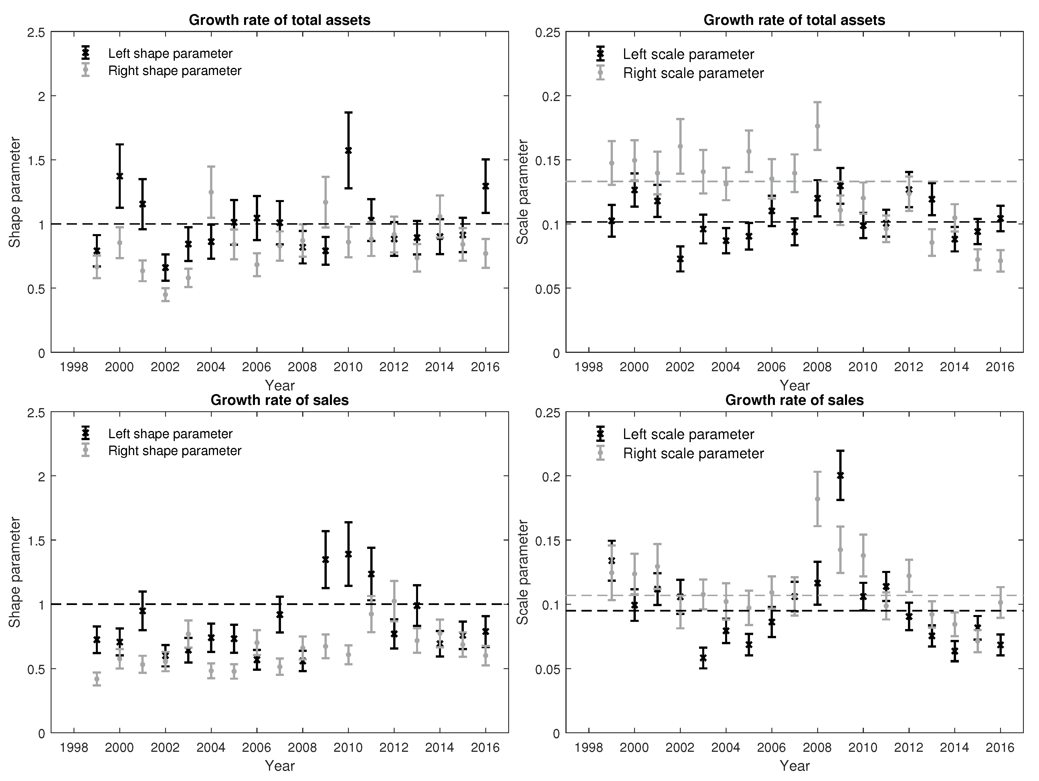
The distribution of growth rates of total assets and sales of the largest long-lived firms (see Figure 8) are characterised by a strong deviation from the Laplace distribution and a high level of volatility, which is in line with the literature (see for instance, [6,13,41]).
Distributional Properties Conditional on Size and Business Cycle Phase
In Figure 9, Figure 10 and Figure 11, we report the estimates of the shape and scale parameters of the AEP computed for profit and growth rates of total assets and sales, conditional on size [see also Table 5 and Table 6].
Regarding profit rates, we observe that and are significantly smaller than 1 most of the years. The shape of the distribution of profit rates depends on the size of the firms becoming fatter the smaller are the firms included in the sample. The scale parameter, instead, shows remarkable stability as a function of the size, with the systematic tendency . This condition changes when we consider the entire sample. The dispersion on the left side, measured by , is higher than the during the phase of the crisis. This change can be attributed to the effect of the business cycle on the profitability of small firms. As can be observed in Table 7 and Table 8, the correlation between the AEP estimated and the GDP growth rates is stronger when including small firms. This result underlines the robustness of the profitability of large firms to the business cycle phase, while the small firms seem to be more affected by the adverse phase of the cycle.
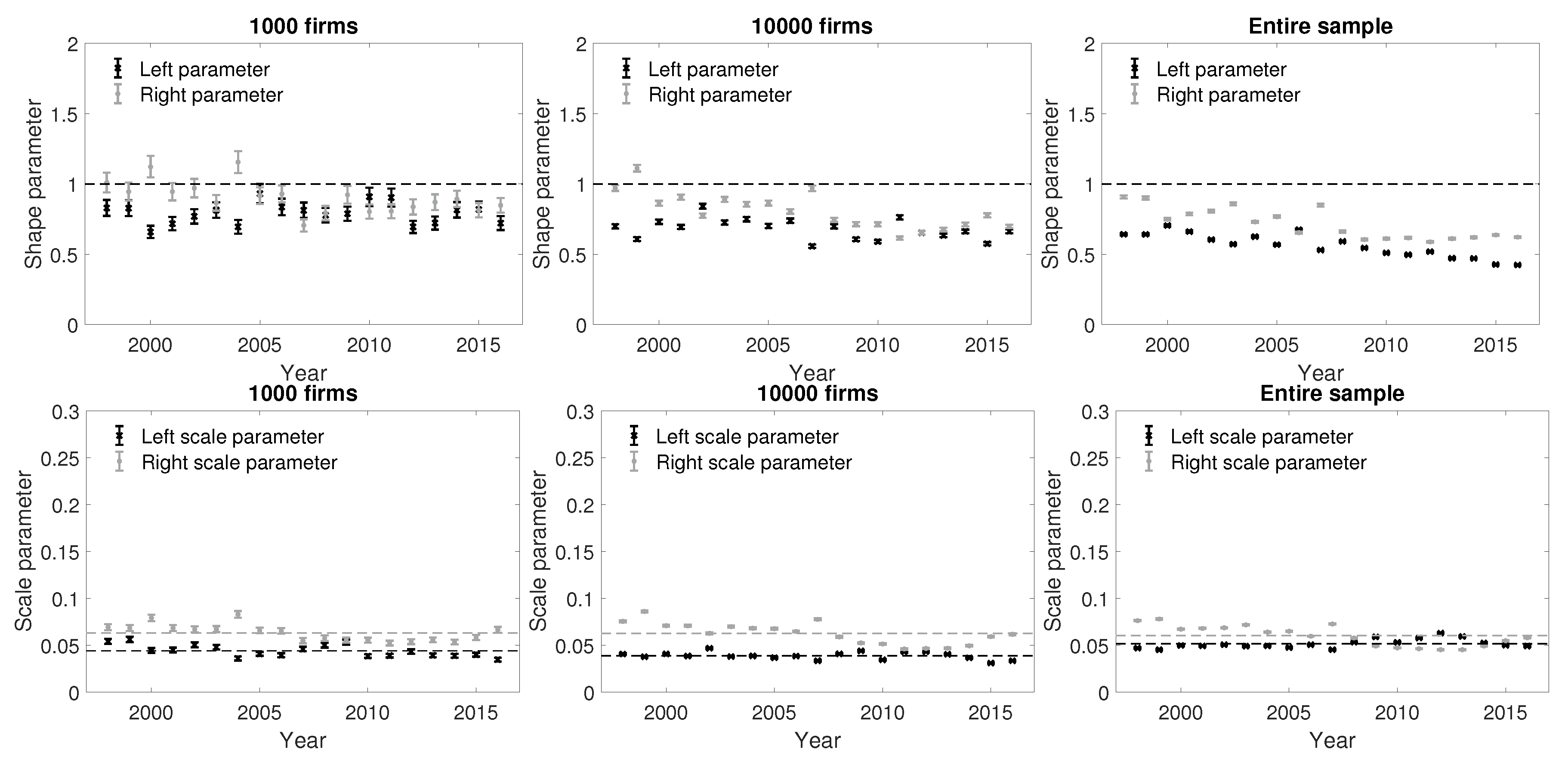
Focusing on growth rates of total assets, we always reject the Laplace distribution hypothesis, due to the differences in the scale parameters and shape parameters, i.e., and . Moreover, the estimates of the shape parameters are different from 1 most of the years. Interestingly, the scale parameters show a similar behaviour to profit rates since the cross-sectional volatility is higher on the right side () for the large firms but, when analysing the entire sample, we identify a remarkable decrease/increase in the cross-sectional volatility on the right/left side during the crisis period.
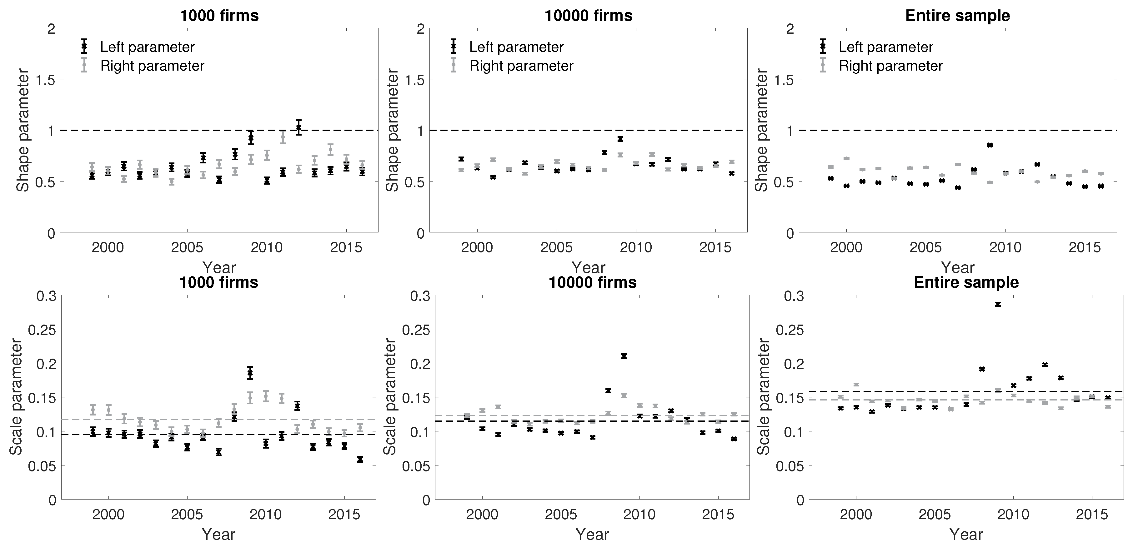
Finally, in relation to growth rates of sales, the Laplace distribution is also rejected since and . When including the smallest firms in the analysis, we observe higher volatility on the left part of the distribution compared to the right one during the downturn, which is consistent with the results reported for profit rates and growth rates of total assets. Thus, with Figure 9, Figure 10 and Figure 11, we are able to underline the effect of the crisis on small firms by means of the scale parameters of profit and growth rates. On the other hand, in relation to the shape parameters, we observe different dynamics between profit and growth rates. More specifically, profit rates tend to be more leptokurtic on both parts of the distribution when including smaller firms on the sample. However, the shape parameters of growth rates on the left part of the distribution become more platikurtic (i.e., we observe a slimming down of the left tail) during the crisis period, compared to the right tail. This particular behaviour has been already reported with the 200 largest long-lived firms (see Figure 8 and Figure A3) in which we observe that during the downturn, growth rates show a higher dispersion on the left part of the distribution with a slimming down of the left tail.
5. Conclusions
In this paper, we shed some light on the firm dynamics literature by analysing to what extent the Laplace distribution describes the Spanish long-lived firms’ distribution of profit and growth rate, against its alternative more general distributions, namely Subbotin and AEP. Moreover, compared to recent literature, we analyse the effect of the different phases of the business cycle and the firm size on the distributional characteristics of profit and growth rates.
We find evidence of systematic deviations of the profit rate distribution from the Laplace benchmark when small firms are included in the analysis. The empirical distribution becomes more leptokurtic without changing the scale parameters. Therefore, the Laplace benchmark turns out to be a reasonable approximation if we limit the sample to large and surviving firms. Relaxing the symmetric constraint, the use of the AEP distribution shows that, instead of a Laplace, the better approximation for firm profit rate distribution is an asymmetric Laplace. Interestingly, except for the location parameter, the shape and scale parameters do not depend on the business cycle phase. Small firms, instead, show a much higher dependence of their profit rates on the business cycle phase, signalling a marked difference with large firms. Taking into account these results, we underline the robustness of the large firms during the financial crisis in terms of profitability given (i) the significant larger dispersion of the right part of the distribution, compared to the left one, and (ii) the absence of relation between the time series of GDP growth rates and the time series of the estimates of , , and for the largest 200 long-lived firms’ profit rates. However, this robustness is lost when including small firms in the sample since (i) we observe that the dispersion of the left part of the distribution is significantly larger than the right one during the years of the downturn, and (ii) the estimates of the entire sample show a remarkable relationship with the GDP growth rates.
On the other hand, focusing on growth rates, we observe a similar tendency compared to profit rates given the effect of the crisis on small firms’ growth distribution (). This result is supported by the stronger correlation between the time series of the estimate parameters and GDP growth rates when including small firms in the sample. Interestingly, we observe that profit and growth rates of total assets show similar dynamics in terms of dispersion, while growth rates of total assets and sales are more similar regarding the shape of the distribution.
Given the results reported in this paper, we infer that the largest firms are more robust to downturns compared to the small firms, due to their invariant distributional characteristics during crisis periods. Consequently, this study provides some insights to policymakers on how turmoil affects firms depending on their size. In particular, the role that the largest firms have on the business cycle is now better understood [26]. Moreover, given that the present analysis is based on a sample of long-lived firms of different sizes, the distributional analysis allows a precise evaluation of the risk related to large downturns in firm profitability conditional on firm size. This information is extremely useful for those investors interested in investing in real economic activity.
Future research could be focused on three directions. First, considering different countries in order to analyse their distributional properties according to their phase in the business cycle. Second, analysing the causal dependencies between the variables of the AEP distribution and GDP growth rates, when longer data sets are available. Finally, we have identified that size is an important factor in the distributional properties of profit and growth rates. However, other firms’ characteristics can be relevant in the dynamics of the distribution (see Mundt et al. (2020) [42]). Thus, in future research, we plan to study the impact of other firm characteristics on the dynamics of the distribution of profit and growth rates.
Author Contributions
All authors have read and agreed to the published version of the manuscript. Conceptualization, D.V.-T., A.R.-B., O.B.-A. and S.A.; Data curation, D.V.-T., A.R.-B., O.B.-A. and S.A.; Formal analysis, D.V.-T., A.R.-B., O.B.-A. and S.A.; Funding acquisition, S.A.; Investigation, D.V.-T., A.R.-B., O.B.-A. and S.A.; Methodology, D.V.-T., A.R.-B., O.B.-A. and S.A.; Supervision, S.A.; Writing—original draft, D.V.-T., A.R.-B., O.B.-A. and S.A.; Writing—review & editing, D.V.-T., A.R.-B., O.B.-A. and S.A.
Funding
The authors are grateful for funding the Universitat Jaume I under the project UJI-B2021-66, the Spanish Ministry of Science, Innovation and Universities under the Project RTI2018-096927-B-I00, the Generalitat Valenciana under the project AICO/2021/005 and the Margarita Salas postdoctoral contract MGS/2021/13 (UP2021-021) financed by the European Union-NextGenerationEU.
Institutional Review Board Statement
Not applicable.
Informed Consent Statement
Not applicable.
Data Availability Statement
Not applicable.
Acknowledgments
The authors are grateful for funding the Universitat Jaume I under the project UJI-B2021-66, the Spanish Ministry of Science, Innovation and Universities under the Project RTI2018-096927-B-I00, the Generalitat Valenciana under the project AICO/2021/005 and the Margarita Salas postdoctoral contract MGS/2021/13 (UP2021-021) financed by the European Union-NextGenerationEU.
Conflicts of Interest
The authors declare no conflict of interest.
Appendix A
Appendix A.1. Firms
Figure A1.
Sales as a function of GDP for the largest long-lived firms in our sample.

Appendix A.2. Likelihood Ratio Test for the 200 Largest Long-Lived Firms
Table A1 and Table A2 show the LRT in which we test the Laplace distribution compared to the AEP as alternative hypothesis. As can be observed, the null hypothesis of the Laplace distribution is rejected most of the years for profit rates and growth rates of total assets and sales. This result supports the outcome observed by Mundt and Oh (2019) [23] since the AEP seems to characterise better the empirical density of profit rates.

Table A1.
P-values of the likelihood ratio test for profit and growth rates of total assets and sales. The null hypothesis is the Laplace distribution, while the alternative hypothesis is the Subbotin distribution. The results refer to the 200 largest long-lived firms according to their sales in 2016. In bold, we underlined P-values below 5%.
| LRT | 1998 | 1999 | 2000 | 2001 | 2002 | 2003 | 2004 | 2005 | 2006 | 2007 |
|---|---|---|---|---|---|---|---|---|---|---|
| Profit rate | 0.17 | 0.05 | 0.04 | 0.16 | 0.06 | 0.11 | 0.21 | 0.06 | 0.01 | 0.00 |
| Total assets | - | 0.00 | 0.00 | 0.00 | 0.00 | 0.00 | 0.05 | 0.00 | 0.00 | 0.01 |
| Sales | - | 0.00 | 0.00 | 0.00 | 0.00 | 0.00 | 0.00 | 0.00 | 0.00 | 0.00 |
| LRT | 2008 | 2009 | 2010 | 2011 | 2012 | 2013 | 2014 | 2015 | 2016 | |
| Profit rate | 0.27 | 0.01 | 0.02 | 0.02 | 0.01 | 0.73 | 0.15 | 0.08 | 0.04 | |
| Total assets | 0.01 | 0.17 | 0.16 | 0.04 | 0.00 | 0.00 | 0.02 | 0.06 | 0.00 | |
| Sales | 0.00 | 0.00 | 0.00 | 0.62 | 0.05 | 0.00 | 0.00 | 0.00 | 0.00 |
Table A2.
P-values of the likelihood ratio test for profit rates and growth rates of total assets and sales. The null hypothesis is the Laplace distribution, while the alternative hypothesis is the AEP distribution. Results refer to the 200 largest long-lived firms, according to their sales in 2016. In bold, we underlined P-values below 5%.
| LRT | 1998 | 1999 | 2000 | 2001 | 2002 | 2003 | 2004 | 2005 | 2006 | 2007 |
|---|---|---|---|---|---|---|---|---|---|---|
| Profit rate | 0.00 | 0.00 | 0.00 | 0.03 | 0.04 | 0.01 | 0.00 | 0.00 | 0.00 | 0.00 |
| Total assets | - | 0.00 | 0.00 | 0.00 | 0.00 | 0.00 | 0.00 | 0.00 | 0.00 | 0.00 |
| Sales | 0.00 | 0.00 | 0.00 | 0.00 | 0.00 | 0.00 | 0.00 | 0.00 | 0.00 | |
| LRT | 2008 | 2009 | 2010 | 2011 | 2012 | 2013 | 2014 | 2015 | 2016 | |
| Profit rate | 0.00 | 0.00 | 0.00 | 0.00 | 0.00 | 0.00 | 0.00 | 0.00 | 0.00 | |
| Total assets | 0.00 | 0.00 | 0.00 | 0.22 | 0.39 | 0.00 | 0.03 | 0.00 | 0.00 | |
| Sales | 0.00 | 0.00 | 0.00 | 0.02 | 0.00 | 0.00 | 0.00 | 0.00 | 0.00 |
Table A3.
P-values of the likelihood ratio test for profit rates and growth rates of total assets and sales. The null hypothesis is the asymmetric Laplace distribution, while the alternative hypothesis is the AEP distribution. Results refer to the 200 largest long-lived firms, according to their sales in 2016. In bold, we underlined P-values below 5%.
| LRT | 1998 | 1999 | 2000 | 2001 | 2002 | 2003 | 2004 | 2005 | 2006 | 2007 |
|---|---|---|---|---|---|---|---|---|---|---|
| Profit rates | 0.57 | 0.01 | 0.40 | 0.39 | 0.56 | 0.58 | 0.01 | 0.00 | 0.39 | 0.15 |
| Total assets | 0.00 | 0.01 | 0.00 | 0.00 | 0.00 | 0.02 | 0.14 | 0.00 | 0.10 | |
| Sales | 0.00 | 0.00 | 0.00 | 0.00 | 0.00 | 0.00 | 0.00 | 0.00 | 0.00 | |
| LRT | 2008 | 2009 | 2010 | 2011 | 2012 | 2013 | 2014 | 2015 | 2016 | |
| Profit rates | 0.01 | 0.01 | 0.00 | 0.29 | 0.58 | 0.07 | 0.81 | 0.43 | 0.01 | |
| Total assets | 0.18 | 0.01 | 0.00 | 0.28 | 0.41 | 0.03 | 0.29 | 0.29 | 0.00 | |
| Sales | 0.00 | 0.00 | 0.00 | 0.08 | 0.03 | 0.00 | 0.01 | 0.00 | 0.00 |
Appendix A.3. Probability Density Function of Growth Rates of Total Assets and Sales
Figure A2.
Probability Density Function (PDF) of growth rates of total assets along with the AEP (dotted line) and Laplace (dashed line) distributions. The results refer to the 200 largest long-lived firms according to their sales in 2016.
Figure A2.
Probability Density Function (PDF) of growth rates of total assets along with the AEP (dotted line) and Laplace (dashed line) distributions. The results refer to the 200 largest long-lived firms according to their sales in 2016.

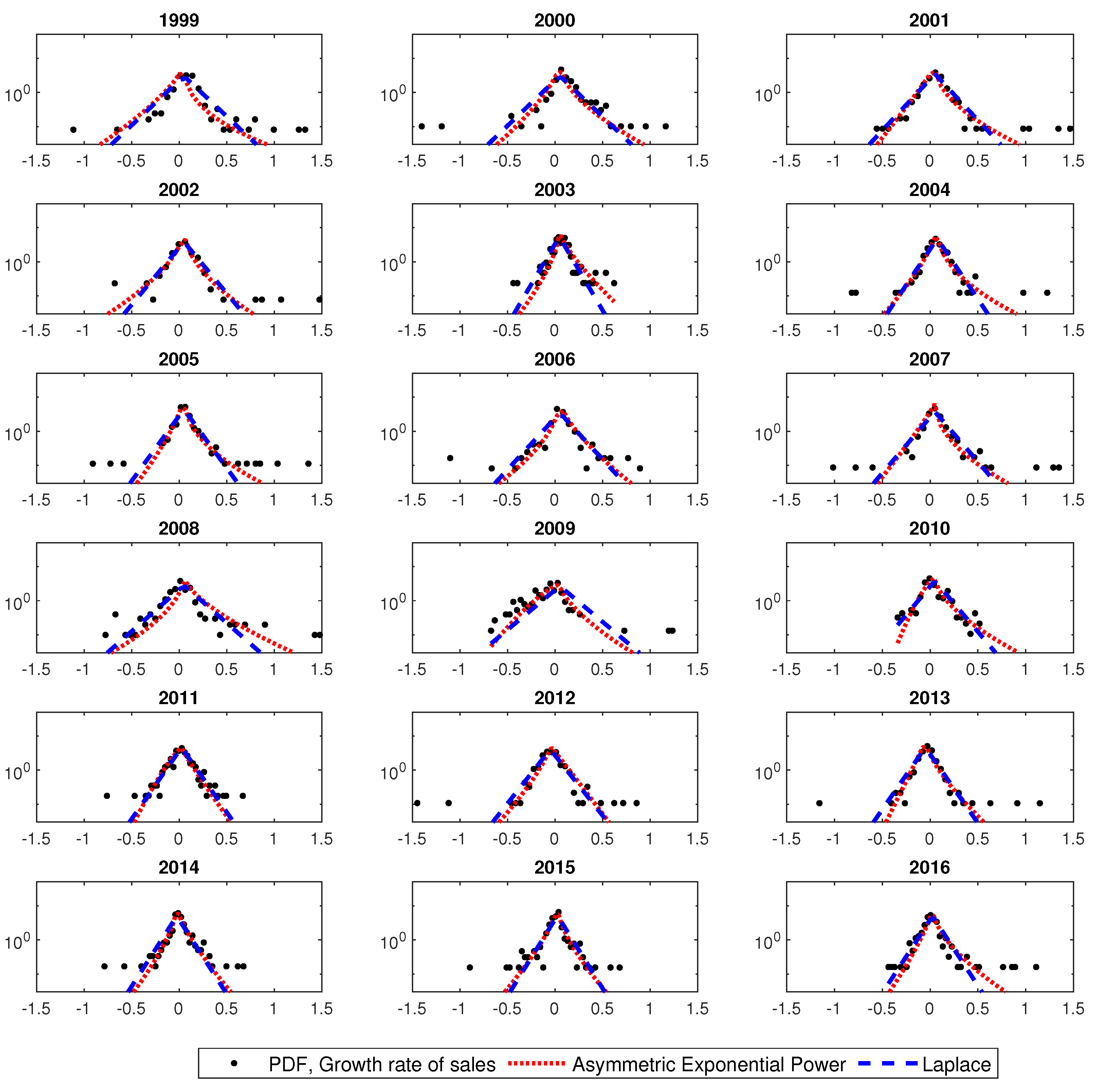
Figure A3.
Probability Density Function (PDF) of growth rates of sales along with the AEP (dotted line) and Laplace (dashed line) distribution. The results refer to the 200 largest long-lived firms according to their sales in 2016.
Figure A3.
Probability Density Function (PDF) of growth rates of sales along with the AEP (dotted line) and Laplace (dashed line) distribution. The results refer to the 200 largest long-lived firms according to their sales in 2016.

References
- Gibrat, R. Les inégalités économiques; Recueil Sirey: Paris, France, 1931. [Google Scholar]
- Sutton, J. Gibrat’s legacy. J. Econ. Lit. 1997, 35, 40–59. [Google Scholar]
- Amaral, N.; Buldyrev, S.L.A.; Havlin, S.; Maass, P.; Salinger, M.; Stanley, H.; Stanley, M. Scaling behavior in economics: The problem of quantifying company growth. Physics A 1997, 244, 1–24. [Google Scholar] [CrossRef]
- Bottazzi, G.; Dosi, G.; Lippi, M.; Pammolli, F.; Riccaboni, M. Innovation and corporate growth in the evolution of the drug industry. Int. J. Ind. Organ. 2001, 19, 1161–1187. [Google Scholar] [CrossRef] [Green Version]
- Bottazzi, G.; Secchi, A. Why are distributions of firm growth rates tent-shaped? Econ. Lett. 2003, 80, 415–420. [Google Scholar] [CrossRef]
- Bottazzi, G.; Secchi, A. Explaining the distribution of firm growth rates. RAND J. Econ. 2006, 37, 235–256. [Google Scholar] [CrossRef]
- Buldyrev, S.V.; Growiec, J.; Pammolli, F.; Riccaboni, M.; Stanley, H.E. The growth of business firms: Facts and theory. J. Eur. Econ. Assoc. 2007, 5, 574–584. [Google Scholar] [CrossRef] [Green Version]
- Alfarano, S.; Milakovic, M. Does classical competition explain the statistical features of firm growth? Econ. Lett. 2008, 101, 272–274. [Google Scholar] [CrossRef] [Green Version]
- Bottazzi, G.; Secchi, A. A new class of asymmetric exponential power densities with applications to economics and finance. Ind. Corp. Chang. 2011, 20, 991–1030. [Google Scholar] [CrossRef] [Green Version]
- Riccaboni, M.; Growiec, J.; Pammolli, F. Innovation and Corporate Dynamics: A Theoretical Framework; University Library of Munich: Munchen, Germany, 2011. [Google Scholar]
- Axtell, R.L. Zipf distribution of us firm sizes. Science 2001, 293, 1818–1820. [Google Scholar] [CrossRef] [Green Version]
- Gaffeo, E.; Gallegati, M.; Palestrini, A. On the size distribution of firms. Additional evidence from the G7 countries. Physics A 2003, 324, 117–123. [Google Scholar] [CrossRef]
- Dosi, G.; Nelson, R.R. Technical change and industrial dynamics as evolutionary processes. Handb. Econ. Innov. 2010, 1, 51–127. [Google Scholar]
- Williams, M.A.; Pinto, B.P.; Park, D. Global evidence on the distribution of firm growth rates. Phys. A Stat. Mech. Its Appl. 2015, 432, 102–107. [Google Scholar] [CrossRef]
- Penrose, E.; Penrose, E.T. The Theory of the Growth of the Firm; Oxford University Press: Oxford, UK, 2009. [Google Scholar]
- Coad, A.; Planck, M. Firms as bundles of discrete resources–towards an explanation of the exponential distribution of firm growth rates. East. Econ. J. 2012, 38, 189–209. [Google Scholar] [CrossRef] [Green Version]
- Alfarano, S.; Milakovic, M.; Albrecht, I.; Kauschke, J. A Statistical Equilibrium Model of Competitive Firms. J. Econ. Dyn. Control 2012, 36, 136–149. [Google Scholar] [CrossRef] [Green Version]
- Mundt, P.; Alfarano, S.; Milaković, M. Gibrat’s Law Redux: Think profitability instead of growth. Ind. Corp. Chang. 2016, 25, 549–571. [Google Scholar] [CrossRef]
- Williams, M.A.; Baek, G.; Park, L.Y.; Zhao, W. Global evidence on the distribution of economic profit rates. Phys. A Stat. Mech. Its Appl. 2016, 458, 356–363. [Google Scholar] [CrossRef]
- Smith, A. An Inquiry into the Nature and Causes of The Wealth of Nations; Harriman House: Petersfield, UK, 1776. [Google Scholar]
- Subbotin, M. On the law of frequency of errors. Matematicheskii Sbornik 1923, 31, 296–301. [Google Scholar]
- Erlingsson, E.J.; Alfarano, S.; Raberto, M.; Stefánsson, H. On the distributional properties of size, profit and growth of Icelandic firms. J. Econ. Interact. Coord. 2013, 8, 57–74. [Google Scholar] [CrossRef] [Green Version]
- Mundt, P.; Oh, I. Asymmetric competition, risk, and return distribution. Econ. Lett. 2019, 179, 29–32. [Google Scholar] [CrossRef] [Green Version]
- Higson, C.; Holly, S.; Kattuman, P. The cross-sectional dynamics of the US business cycle: 1950–1999. J. Econ. Dyn. Control 2002, 26, 1539–1555. [Google Scholar] [CrossRef]
- Higson, C.; Holly, S.; Kattuman, P.; Platis, S. The Business Cycle, Macroeconomic Shocks and the Cross-Section: The Growth of UK Quoted Companies. Economica 2004, 71, 299–318. [Google Scholar] [CrossRef] [Green Version]
- Gabaix, X. The granular origins of aggregate fluctuation. Econometrica 2011, 79, 733–772. [Google Scholar]
- Bottazzi, G.; Li, L.; Secchi, A. Aggregate fluctuations and the distribution of firm growth rates. Ind. Corp. Chang. 2019, 28, 635–656. [Google Scholar] [CrossRef] [Green Version]
- Haltiwanger, J.C. Measuring and analyzing aggregate fluctuations: The importance of building from microeconomic evidence. Fed. Reserve Bank St. Louis Rev. 1997, 79, 55. [Google Scholar] [CrossRef]
- Geroski, P.A.; Gregg, P. Coping with Recession: UK Company Performance in Adversity; Cambridge University Press: Cambridge, UK, 1997; Volume 38. [Google Scholar]
- De Veirman, E.; Levin, A. Cyclical Changes in Firm Volatility; Technical Report; The Australian National University: Canberra, Australia, 2011. [Google Scholar]
- Holly, S.; Petrella, I.; Santoro, E. Aggregate fluctuations and the cross-sectional dynamics of firm growth. J. R. Stat. Soc. Ser. A 2013, 176, 459–479. [Google Scholar] [CrossRef] [Green Version]
- Bachmann, R.; Bayer, C. Investment dispersion and the business cycle. Am. Econ. Rev. 2014, 104, 1392–1416. [Google Scholar] [CrossRef] [Green Version]
- Blanco-Arroyo, O.; Ruiz-Buforn, A.; Vidal-Tomás, D.; Alfarano, S. On the determination of the granular size of the economy. Econ. Lett. 2018, 173, 35–38. [Google Scholar] [CrossRef] [Green Version]
- Blanco-Arroyo, O.; Ruiz-Buforn, A.; Vidal-Tomás, D.; Alfarano, S. Granular companies and regional breakdown: An analysis of the Spanish case. Stud. Appl. Econ. 2019, 37, 109–124. [Google Scholar]
- Stanley, M.; Amaral, L.; Buldyrev, S.; Havlin, S.; Leschhorn, H.; Maass, P.; Salinger, M.; Stanley, H. Scaling behaviour in the growth of companies. Nature 1996, 379, 804–806. [Google Scholar] [CrossRef]
- Mundt, P.; Förster, N.; Alfarano, S.; Milakovic, M. The real versus the financial economy: A global tale of stability versus volatility. Econ. Open-Access Open-Assess. E-J. 2014, 8, 1–26. [Google Scholar] [CrossRef] [Green Version]
- Coad, A.; Segarra, A.; Teruel, M. Like milk or wine: Does firm performance improve with age? Struct. Chang. Econ. Dyn. 2013, 24, 173–189. [Google Scholar] [CrossRef] [Green Version]
- Jaynes, E.T. Where do we stand on maximum entropy? In E.T. Jaynes: Papers on Probability, Statistics and Statistical Physics; Rosenkrantz, R.D., Ed.; Kluwer Academic Publishers: Dordrecht, The Netherlands, 1978. [Google Scholar]
- Bottazzi, G.; Secchi, A.; Tamagni, F. Financial constraints and firm dynamics. Small Bus. Econ. 2014, 42, 99–116. [Google Scholar] [CrossRef]
- Bottazzi, G. Subbotools User’s Manual: For Version 0.9. 7.1, 8 September 2004; Technical Report, LEM Working Paper Series; Laboratory of Economics and Management (LEM): Pisa, Italy, 2004; Available online: https://www.researchgate.net/publication/24132325_Subbotools_User (accessed on 8 March 2022).
- Fu, D.; Pammolli, F.; Buldyrev, S.V.; Riccaboni, M.; Matia, K.; Yamasaki, K.; Stanley, H.E. The growth of business firms: Theoretical framework and empirical evidence. Proc. Natl. Acad. Sci. USA 2005, 102, 18801–18806. [Google Scholar] [CrossRef] [Green Version]
- Mundt, P.; Alfarano, S.; Milaković, M. Survival and the Ergodicity of Corporate Profitability; BERG Working Paper Series 162; Bamberg University: Bamberg, Germany, 2020. [Google Scholar]
Figure 1.
(a,b) The evolution of the cross-sectional median and standard deviation of growth () and profit rates for the 200 largest long-lived firms, respectively (base year 2016). (c,d) The evolution of the cross-sectional median and standard deviation of growth () and profit rates for the entire sample at our disposal, respectively (base year 2016).

Figure 2.
Estimates of the shape and scale parameter of the Subbotin distribution for profit rates. Error bars show two standard errors. The results refer to the 200 largest long-lived firms according to their sales in 2016. The dashed line in the scale parameter figure represents the median of the estimates.

Figure 3.
Probability Density Function (PDF) of profit rates along with the AEP (dotted line) and Laplace (dashed line) distribution. The results refer to the 200 largest long-lived firms according to their sales in 2016.
Figure 3.
Probability Density Function (PDF) of profit rates along with the AEP (dotted line) and Laplace (dashed line) distribution. The results refer to the 200 largest long-lived firms according to their sales in 2016.

Figure 4.
Estimates of the shape and scale parameter of the Subbotin distribution for growth rates of total assets and sales. Error bars show two standard errors. The results refer to the 200 largest long-lived firms according to their sales in 2016. The dotted line (sales) and dashed line with dots (total assets) in the scale parameter figure represent the median of the estimates.

Figure 5.
Estimates of the shape parameter of the Subbotin distribution of profit rates, growth of total assets and sales. Error bars show two standard errors. Results refer to the largest long-lived firms of our sample according to their sales in 2016.
Figure 5.
Estimates of the shape parameter of the Subbotin distribution of profit rates, growth of total assets and sales. Error bars show two standard errors. Results refer to the largest long-lived firms of our sample according to their sales in 2016.

Figure 6.
Estimates of the scale parameter of the Subbotin distribution for profit rates, growth of total assets and sales. Error bars show two standard errors. Results refer to the largest long-lived firms of our sample according to their sales in 2016. The dashed line (profit), dotted line (sales) and dashed line with dots (total assets) in the scale parameter figure represent the median of the estimates.

Figure 7.
Estimates of the two shape parameters ( and ) and two scale parameters ( and ) for the profit rates distribution. The results refer to the 200 largest long-lived firms according to their sales in 2016. Gray and black dashed lines refer to the median of the estimates of and , respectively.
Figure 7.
Estimates of the two shape parameters ( and ) and two scale parameters ( and ) for the profit rates distribution. The results refer to the 200 largest long-lived firms according to their sales in 2016. Gray and black dashed lines refer to the median of the estimates of and , respectively.

Figure 8.
Estimates of the two shape parameters ( and ) and two scale parameters ( and ) for growth rates of total assets and sales. Results refer to the 200 largest long-lived firms according to their sales in 2016. Gray and black dashed lines refer to the median of the estimates of and , respectively.

Figure 9.
Estimates of the two shape parameters ( and ) and two scale parameters ( and ) of the AEP distribution for profit rates conditional on size. Error bars show two standard errors. Gray and black dashed lines refer to the median of the estimates of and , respectively.
Figure 9.
Estimates of the two shape parameters ( and ) and two scale parameters ( and ) of the AEP distribution for profit rates conditional on size. Error bars show two standard errors. Gray and black dashed lines refer to the median of the estimates of and , respectively.

Figure 10.
Estimates of the two shape parameters ( and ) and two scale parameters ( and ) of the AEP distribution for growth rates of total assets conditional on size. Error bars show two standard errors. Gray and black dashed lines refer to the median of the estimates of and , respectively.
Figure 10.
Estimates of the two shape parameters ( and ) and two scale parameters ( and ) of the AEP distribution for growth rates of total assets conditional on size. Error bars show two standard errors. Gray and black dashed lines refer to the median of the estimates of and , respectively.

Figure 11.
Estimates of the two shape parameters ( and ) and two scale parameters ( and ) of the AEP distribution for growth rates of sales conditional on size. Error bars show two standard errors. Gray and black dashed lines refer to the median of the estimates of and , respectively.
Figure 11.
Estimates of the two shape parameters ( and ) and two scale parameters ( and ) of the AEP distribution for growth rates of sales conditional on size. Error bars show two standard errors. Gray and black dashed lines refer to the median of the estimates of and , respectively.

Table 1.
P-values of the likelihood ratio test for profit and growth rates of total assets and sales. The null hypothesis is the Laplace distribution, while the alternative hypothesis is the Subbotin distribution. The results refer to the 200 largest long-lived firms, according to their sales in 2016, when deleting the extreme positive and negative value. In bold, we underlined P-values below 5%.
| LRT | 1998 | 1999 | 2000 | 2001 | 2002 | 2003 | 2004 | 2005 | 2006 | 2007 |
|---|---|---|---|---|---|---|---|---|---|---|
| Profit rate | 0.87 | 0.93 | 0.39 | 0.64 | 0.81 | 0.58 | 0.95 | 0.53 | 0.20 | 0.14 |
| Total assets | - | 0.00 | 0.77 | 0.01 | 0.00 | 0.00 | 0.57 | 0.05 | 0.05 | 0.09 |
| Sales | - | 0.00 | 0.00 | 0.00 | 0.00 | 0.00 | 0.00 | 0.00 | 0.00 | 0.00 |
| LRT | 2008 | 2009 | 2010 | 2011 | 2012 | 2013 | 2014 | 2015 | 2016 | |
| Profit rate | 0.61 | 0.04 | 0.35 | 0.29 | 0.19 | 0.61 | 0.72 | 0.88 | 0.93 | |
| Total assets | 0.11 | 0.42 | 0.84 | 0.77 | 0.42 | 0.08 | 0.86 | 0.29 | 0.15 | |
| Sales | 0.00 | 0.01 | 0.01 | 0.48 | 0.35 | 0.01 | 0.01 | 0.01 | 0.00 |
Table 2.
Median of the estimates of the shape parameter reported in Figure 5.
Table 2.
Median of the estimates of the shape parameter reported in Figure 5.
| N° Firms | Profit Rate | TA | Sales |
|---|---|---|---|
| 200 | 0.94 | 0.88 | 0.70 |
| 1000 | 0.83 | 0.79 | 0.67 |
| 10,000 | 0.74 | 0.79 | 0.66 |
| Entire sample | 0.66 | 0.72 | 0.58 |
Table 3.
Median of the estimates of the scale parameter reported in Figure 6.
Table 3.
Median of the estimates of the scale parameter reported in Figure 6.
| N° Firms | Profit Rate | TA | Sales |
|---|---|---|---|
| 200 | 0.055 | 0.123 | 0.105 |
| 1000 | 0.054 | 0.122 | 0.112 |
| 10,000 | 0.053 | 0.119 | 0.117 |
| Entire sample | 0.055 | 0.130 | 0.145 |
Table 4.
Pearson correlation coefficient between the time series of the estimates of m, and with the time series of GDP growth rates. *** denotes significance at the 1% level; ** denotes significance at the 5% level; * denotes significance at the 10% level.
Table 4.
Pearson correlation coefficient between the time series of the estimates of m, and with the time series of GDP growth rates. *** denotes significance at the 1% level; ** denotes significance at the 5% level; * denotes significance at the 10% level.
| m & GDP | & GDP | & GDP | |||||||
|---|---|---|---|---|---|---|---|---|---|
| N° of Firms | Profit Rates | TA | Sales | Profit Rates | TA | Sales | Profit Rates | TA | Sales |
| 200 | 0.51 ** | 0.27 | 0.48 ** | 0.07 | −0.38 | −0.76 *** | 0.00 | 0.38 | −0.14 |
| 1000 | 0.36 | 0.64 *** | 0.58 ** | 0.37 | −0.51 ** | −0.68 *** | 0.69 *** | 0.46 ** | −0.25 |
| 10,000 | 0.59 *** | 0.81 *** | 0.59 *** | 0.79 *** | −0.21 | −0.50 ** | 0.78 *** | 0.70 *** | −0.59 *** |
| Entire sample | 0.63 *** | 0.93 *** | 0.92 *** | 0.83 *** | 0.40 | −0.36 | 0.74 *** | 0.76 *** | −0.76 *** |
| N° of Firms | Profit Rates | TA | Sales | Profit Rates | TA | Sales |
| 200 | 1.00 | 0.91 | 0.75 | 0.93 | 0.84 | 0.63 |
| 1000 | 0.81 | 0.74 | 0.60 | 0.89 | 0.81 | 0.65 |
| 10,000 | 0.69 | 0.79 | 0.63 | 0.78 | 0.80 | 0.65 |
| Entire sample | 0.57 | 0.68 | 0.50 | 0.66 | 0.75 | 0.59 |
| N° of Firms | Profit Rates | TA | Sales | Profit Rates | TA | Sales |
| 200 | 0.04 | 0.10 | 0.09 | 0.06 | 0.13 | 0.11 |
| 1000 | 0.04 | 0.09 | 0.09 | 0.07 | 0.14 | 0.11 |
| 10,000 | 0.04 | 0.10 | 0.11 | 0.06 | 0.13 | 0.12 |
| Entire sample | 0.05 | 0.10 | 0.14 | 0.06 | 0.14 | 0.15 |
Table 7.
Pearson correlation coefficient between the time series of the estimates of and with the time series of GDP growth rates. *** denotes significance at the 1% level; ** denotes significance at the 5% level; * denotes significance at the 10% level.
Table 7.
Pearson correlation coefficient between the time series of the estimates of and with the time series of GDP growth rates. *** denotes significance at the 1% level; ** denotes significance at the 5% level; * denotes significance at the 10% level.
| & GDP | & GDP | |||||
|---|---|---|---|---|---|---|
| N° of Firms | Profit Rates | TA | Sales | Profit Rates | TA | Sales |
| 200 | 0.35 | 0.05 | −0.61 *** | 0.07 | −0.43 | −0.68 *** |
| 1000 | −0.04 | −0.04 | −0.49 ** | 0.4 | −0.4 | −0.61 *** |
| 10,000 | 0.33 | 0.16 | −0.52 ** | 0.77 *** | −0.02 | −0.35 |
| Entire sample | 0.63 *** | −0.33 | −0.72 *** | 0.78*** | 0.83 *** | 0.71 *** |
Table 8.
Pearson correlation coefficient between the time series of the estimates of and with the time series of GDP growth rates. *** denotes significance at the 1% level; ** denotes significance at the 5% level; * denotes significance at the 10% level.
Table 8.
Pearson correlation coefficient between the time series of the estimates of and with the time series of GDP growth rates. *** denotes significance at the 1% level; ** denotes significance at the 5% level; * denotes significance at the 10% level.
| & GDP | & GDP | |||||
|---|---|---|---|---|---|---|
| N° of Firms | Profit Rates | TA | Sales | Profit Rates | TA | Sales |
| 200 | 0.07 | −0.38 | −0.30 | 0.21 | 0.54 ** | −0.11 |
| 1000 | 0.12 | −0.14 | −0.46 * | 0.73 *** | 0.58 ** | −0.35 |
| 10,000 | −0.26 | 0.11 | −0.61 *** | 0.86 *** | 0.83 *** | −0.45 * |
| Entire sample | −0.88 **** | −0.21 | −0.81 *** | 0.89 *** | 0.87 *** | 0.00 |
Publisher’s Note: MDPI stays neutral with regard to jurisdictional claims in published maps and institutional affiliations. |
© 2022 by the authors. Licensee MDPI, Basel, Switzerland. This article is an open access article distributed under the terms and conditions of the Creative Commons Attribution (CC BY) license (https://creativecommons.org/licenses/by/4.0/).
Share and Cite
MDPI and ACS Style
Vidal-Tomás, D.; Ruiz-Buforn, A.; Blanco-Arroyo, O.; Alfarano, S. A Cross-Sectional Analysis of Growth and Profit Rate Distribution: The Spanish Case. Mathematics 2022, 10, 926. https://0-doi-org.brum.beds.ac.uk/10.3390/math10060926
AMA Style
Vidal-Tomás D, Ruiz-Buforn A, Blanco-Arroyo O, Alfarano S. A Cross-Sectional Analysis of Growth and Profit Rate Distribution: The Spanish Case. Mathematics. 2022; 10(6):926. https://0-doi-org.brum.beds.ac.uk/10.3390/math10060926
Chicago/Turabian StyleVidal-Tomás, David, Alba Ruiz-Buforn, Omar Blanco-Arroyo, and Simone Alfarano. 2022. "A Cross-Sectional Analysis of Growth and Profit Rate Distribution: The Spanish Case" Mathematics 10, no. 6: 926. https://0-doi-org.brum.beds.ac.uk/10.3390/math10060926
Note that from the first issue of 2016, this journal uses article numbers instead of page numbers. See further details here.