Mathematical Modelling of Inventory and Process Outsourcing for Optimization of Supply Chain Management

Abstract

Outsourcing is one of the major challenges for production firms in the current supply chain management (SCM) due to limited skilled workers and technology resources. There are too many parameters involved in the strategic decisions of the outsourcing level, quantity, quality, and cost. The outsourcing process removes the burden of capital investment; however, still it creates crucial concerns related to inventory control and production management by adding extra inventories. The semi-finished products are outsourced for a few processes due to limited resources and then returned to the manufacturer for the finishing operations. The article is based on the mathematical modeling and optimization of the process outsourcing considering imperfect production with variable quantity for the effective supply chain management. The numerical experiment was performed based on the data taken from the industry for the application of the proposed outsourcing-based SCM model. The results are significant in finding optimal production and outsourcing quantity with a minimum total cost of SCM. The sensitivity analysis was performed to see how important the effect of input parameters is on the total cost. The research is an important contribution in developing a mathematical model of process outsourcing in SCM. The research study is beneficial for managers to find the economic feasibility of process outsourcing for managing inventory and supply chain between manufacturer and outsourcing vendor.

1. Introduction

In the present socio-economic scenario, outsourcing is a dominant production mode that is rampant around the globe. To compete in this technologically advanced age, the market is saturated in terms of product variety and product life cycle [1]. Further, to take advantage of the competitor, an organization must focus on specialized processes and outsource other activities [2]. Nowadays, it is difficult to meet all customers’ needs; therefore, the basic objective of outsourcing should be flexibility enhancement and letting the organization focus on their specialized activities [3]. Initially, firms would usually outsource the non-specialized activities, but how each activity can be outsourced irrespective of the specialized or non-specialized activity has changed with the times [4].

Outsourcing has become the prime attention of organizations due to several advantages, e.g., low initial investment, reduction of cost, and enhanced customer services [2]. In the basic production order quantity model, it is assumed that a complete lot of products that are produced are non-defective; however, in real-life productions, there are some defective items. These defective products are discarded, while others are reprocessed to ensure good-quality products. An example of outsourcing is an anime figure designing company in Japan that outsources its production activities to its CM. They outsource the coloring process, which is a difficult task and usually takes more time to complete the duplicated figure. The CM to which this company outsources its activities reduces the estimated amount by about 25%.

Outsourcing in a supply chain (SC) is an epithet of economic globalization, which, on the other hand, decentralizes the SC and encounters the OPM with uncertainty. A few years back, a survey conducted by Deloitte depicted that almost 71% of a pool of 600 executives from worldwide companies observe SC risk as a significant factor affecting the company’s strategic decisions [5]. Particularly, the original product manufacturer (OPM) designs a new product due to technological advantage in developed countries. Later on, it outsources its manufacturing to a contract manufacturer from a developing country. The advantages are obvious, such as freeing up the capital, labor cost reduction, and worker productivity [6].

Several researchers have attempted to deal with yield uncertainty in which they have typically used multiplicative fashion to model it. However, these researchers have assumed a case in which the items produced are exactly equal to the ordered quantity, which is physically not always possible. A production environment that follows make-to-order scenario may face a lack of the Requisite products. Still, there is certain research work in which the researchers have picked production and order quantity of their own choice [7,8]. In these cases, the optimization of both the production as well as of order quantity is equally important. Several researchers have done work on product outsourcing, but very little work is available on process outsourcing and its mathematical model’s development. The purpose of this project takes into consideration the process of outsourcing in an imperfect environment for optimization to minimize the cost. Organizations with restricted resources require outsourcing to satisfy customer demands. Additionally, in the proposed research, the mathematical models for the supply chain are developed and tested using the data, which provides a platform to the decision makers to minimize total cost by optimizing the lot size and outsourcing quantity.

Due to certain restrictions, i.e., production programing in some SMEs, which produces some kind of special products as per make-to-order policy or manufacture commodities, reprocessing of imperfect products is not possible. Therefore, such organizations outsource the reprocessing of these imperfect products to some other firms, i.e., repair stores. Moreover, reprocessing these imperfect products, some specific operations i.e., welding, milling/lath machines, or any other kind of equipment that may not be available at the facility and purchasing of that equipment, may not reasonable. On the other hand, imperfect products have a significant value to a company, and therefore, the rework of imperfect items is outsourced. It is assumed that in the after-repair process, the products are as good as perfect ones, especially in the case of remanufacturing. It is considered that the HC of repaired products is higher than the initial HC [9,10,11]. Additionally, it is assumed that in a repair shop, the repair process is always under control, and all the imperfect products can be repaired. Furthermore, the repaired items are added to inventory in the same production cycle.

2. Literature

Outsourcing is considered as a prime factor to gain the best possible performance by an organization [12]. For flexible, low-cost production in a supply chain, outsourcing from suppliers is critical. In this regard, better supplier selection as an outsourcer is important. Kumar et al. developed a logical method in which, for multi-objective modeling, they used three different types of fuzzy logic and some hard constraints. In addition to this, they also opted for goal programming for the problem solution [13]. To simultaneously find the order quantity and formulation impression, more sophisticated fuzzy multi-objective methods have been considered by [14]. In another study, [15] developed a model in which the consumer needs to determine the goods that need to be ordered, the amounts, the suppliers, and the times. To find the best suppliers and how to assign orders among them, Karpak et al. [16] used goal programming, evaluating trade-offs between multiple objectives, such as cost, quality, and delivery, simultaneously.

Next, outsourcing strategies are also one of the important aspects of production business schemes of specific operations. While outsourcing some of their operations, the organizations can have a special focus on their core operations. In conventional outsourcing, only the non-specialized activities are outsourced except the activities that may have a competitive advantage [17,18,19]. In a production environment, different researchers have modeled several optimal batch problems considering different production conditions to minimize the total system cost. For instance, E.W. Taft [20] is among the pioneers who developed Economic Production quantity (EPQ) inventory model. Subsequently, this basic model was modified and expanded by other researchers. Previous research studies have shown that small perturbations in parameters of EOQ and EPQ models do not impose any significant impact on the solution of a problem. Owing to this, the Economic Production quantity (EPQ) model emerged as an optimal substitute, which shows promising results for a production environment when applied with some assumptions.

In an actual production environment, the system runs with some imperfections. The imperfections in a production system produce low-quality items for several reasons, namely defects in raw materials, changes in machine capabilities, backorders, rework, and differences in the experience of the operators. Some research studies are available in the literature in which the proposed models have considered these imperfections. For example, Jamal et al. [21] studied the EPQ model to obtain the optimum Batch size. The proposed model is considered a re-work process after several production cycles. Expanding the contributions of Jamal et al. [21], Sarkar et al. [22] formulated the same problem with additional terms of backorders. The model proposed by Cardenas-Barron [23] encompasses numerous parameters. The model undertakes the reworked production quantities and other production system defects. Wee et al. [24] adopted the same methodology and developed a model that considered the development of refurnished products with non-conformities. It was concluded that in repeated manufacturing cycles, there is an effective way to reprocess faulty products. The data obtained confirmed the critical aspects could be more related to the manufacturing cost and the service expenditures of the process. An identical model was presented by [25], which focused on the inflation effect. It was shown that the prolonged use of the manufacturing units could potentially damage the smooth operating of the system, i.e., could produce defects in the system. The focus of the research was on how to overcome the defects produced during the smooth operation and to reprocess the defective products. The overtime of the workers could be the potential reason for the introduction of defects into the system, or it could be due to unrealized reasons. Lastly, the study of Talizadeh et al. [26] is emphatic towards dealing with imperfection in an outsourcing supply chain environment.

Another factor in outsourcing is optimally tweaking the resources. In this area, Alvarez and Stenbacka [27] and Benaroch et al. [28] researched flexible sourcing models for finding the optimal expected time to change resources. The outsourcing cost per transaction in their considered dynamic models is variable. Inderfurth and Kelle [29] and Spinler and Huchzermeier [30] took the outsourcing strategy when both cost and demand are not certain. Liu and Nagurney [31] put forward a model with a global outsourcing and quick-response mechanism. Vibrational inequality theory was used for investigation by considering uncertainty in cost and demand. Some cases were analyzed to take both demand and production costs into account. Nosoohi and Nookabadi [32] developed a model of outsourcing for the industrialist to study optimal ordering policy under the uncertainty of customer demand and final processing costs. They used different options contracts for neutralizing the effect of uncertainty in cost parameters. Chen et al. [33] studied the outsourcing and coordination mechanism for two Stackelberg game models by considering numerous uncertainty parameters, such as disruption risk, demand, and capacity. They concluded that the manufacturer will not be interested in outsourcing if the disruption-risk/production capacity is low/high. Zhao et al. [34] studied a situation where an industrialist outsources a portion of his production to a supplier. They considered the ordering behavior of companies that outsource their products over long distances. Min [35] considered the usual outsourcing techniques of logistics operations in factories of the United States and recognized the significant elements of outsourcing in logistics operations.

Research has also been carried out on outsourcing risk from various perspectives. Lacity et al. [36] stated that risk is the degree to which a transaction exposes a party to a chance of damage or loss. Qin et al. [37] studied the risks linked with ITO in Chinese institutions and concluded that mismatch in culture and goals, limited choice of vendors, and IT literacy are the significant risks. Oh et al. [38] utilized the stock market’s reaction to study the perceived transactional risks linked with ITO engagement. They determined the market’s reaction based on the cultural similarity with the vendor and the asset specification of the IT resources. Earl [39] pinpointed the role of inexperienced staff, lack of innovation, organizational learning, and hidden costs as risks in outsourcing. Gewald and Dibbern [40] determined the levels of perceived risk as well as benefits for finding the extent to which banks would select to outsource their processes.

Research on service outsourcing has been carried out widely by different researchers. Choi et al. [41] performed research and suggested service outsourcing as a critical topic in service supply chain management. Tsai et al. [42] examined the potential risks structural relationships that can lead to failure in an outsourcing relationship. Typically, business is linked with forward and reverse flows of products. Yet, customers are vastly involved in the service process. The valuation of the service level is critical to the market demand [43]. Nowadays, outsourcing is a major development in the service industry for increasing the level of service. Chen et al. [44] considered an outsourced supply chain that consists of one original equipment manufacturer, one contract manufacturer, and a retailer. They studied the results of encroachment on the profit. Akan et al. [45] investigated two outsourcing settings, namely order fulfillment and call center, and examined how asymmetric demand information will affect the two parties. Xin et al. [46] compared the proactive inventory of relief items both in the presence and absence of outsourcing. They concluded that social efficiency improvement depends on the monitoring costs and the perishable rates under the outsourcing strategy. Wu et al. [47] investigated the incentives for information shared with two retailers in Cournot competition and with multiple suppliers in Bertrand competition. Li et al. [48] also studied the service channel choice. Huang et al. [49] investigated the quality risk from the viewpoint of a 4PL and considered asymmetric information in between 3PL and 4PL. Zhang et al. [50] discussed the retailer’s information-sharing strategies when the service is delegated to the retailer or undertaken by the manufacturer. Yue and Ryan [51] carried out a comparison between single sourcing and multi-sourcing. They found that buyers always desire single sourcing to multi-sourcing. Ching et al. [52] used time-based competition for analyzing the model of outsourcing to multiple make-to-order suppliers. Ding et al. [53] used the customized integration service chain model for evaluating the business performance and found that it extends the service supply chain with multiple service providers in the oilfield service industry. Summing up the literature on outsourcing, an ample amount of work has been done by various researchers in service as well as manufacturing streams considering imperfection, outsourcing strategies, supplier selection, risk assessments of outsourcing products, etc., as illustrated in

Table 1. Authors Contribution.

Author	Corporate SC	Outsourcing		Recycling	Imperfection	Outsource		Modeling
		Process	Product			Single	Multiple
Ching et al. [51]			x				x	x
Ding et al. [52]		x					x
Yue and Ryan [50]	x		x	x		x	x	x
Choi et al. [40]	x		x				x
Stenbacka [26]	x		x		x		x	x
Nosoohi and Nookabadi [31]	x		x					x
Chen et al. [32]	x		x	x	x	x
Talizadeh et al. [26]	x		x		x	x	x	x
Proposed Study	x	x		x	x	x		x

. However, mathematical modelling of outsourcing the processes with attributes of imperfection and recycling has not been pondered by any researcher, and this work provides insight into this gap.

3. Mathematical Modelling

A supply chain management model was developed, considering manufacturer and multi-vendor, to deal with the inventory and production control by modelling process outsourcing operation. The assumptions, notations, and model formulation are part of mathematical modelling. The centralized inventory diagram of the proposed mathematical model is given in Figure 1.

3.1. Assumptions

Before proceeding with the modeling, the following assumptions are considered:

• Due to a lack of in-house resources, the manufacturer outsources certain operations;
• The demand of customers is only fulfilled in phase 3;
• The demand and production rates are known and constant;
• A single type of item is considered in the model;
• Raw material holding cost per unit item is smaller than the unit holding cost of work in process;
• Phase A has a higher production rate than phase 2, which is higher than phase 3; therefore, there are no shortages. (P₁ > ∑ P_vi > P₃ > D);
• The inspection is performed during the production and rework phase;
• The scrape is zero in the production phase as well as in the rework phase;
• The rate of reworking is the same as the production rate;
• Inventory holding cost is based on the average inventory;
• The screening cost is considered negligible in this model.

As shown in Figure 1, there are three production phases to the inventory diagram. Manufacturer activities are included in phase 3, whereas outsourcing processes are represented in phase 2. T₁, T₂, and T₃ are the three portions of the total time T, which are further subdivided into t₁, t₂, t₃, t₄, t₅, t₆, t₇, t₈, and t₉. The customer demand rate is denoted by “D”. In the first and third phases I_max1 and I_max3 represent maximum inventories, I_max11 and I_max31 represent the inventories produced after the rework of defective parts, and I_max12 and I_max32 indicates production Quantities without defective items. In the second phase, I_max2i indicates the maximum inventory level of the ith outsourcer, I_max2i1 indicates inventory produced after the rework of defective parts for ith outsourcer, and I_max2i2 indicates ith outsourcer production quantity without defective items. The manufacturer produced amount Q₁ in the first phase, which is distributed into n number of vendors in optimal Quantities Q₂₁, Q₂₂, …, Q_2n. In the second step, vendors perform operations and send it back to the manufacturer. Finally, the products enter the manufacturer’s third phase, where they are turned into final products and distributed to customers.

3.2. Notation

The decision variables are “Q, Q₁, Q₂, Q₃, …, Q_n”. Q is the production quantity for manufacture. Q₁ is the production quantity for the first vendor, Q₂ is the production quantity for the second vendor, and Q₃ is the production quantity for the third vendor, while Q_n is the production quantity for nth vendor. To express the mathematical model discussed in this study, certain notations were adopted in this research. The table below contains and explains these notations.

3.3. Modelling

The SCM model is divided into three phases (first, second, and third phases). Raw material inventory decreases when production starts during time t₁, t₄, and t₇ in phases 1, 2, and 3, respectively, and similarly, the quantity of products continues increasing and approaching its maximum level. The first and the last phase is of the manufacturer and the second phase include all vendors. The demand of the customer is fulfilled only in the third phase. The objective function of our model is to minimize the total cost of supply chain TC, which is equal to the total cost of the manufacturer and total cost of vendors.

$$TC=T{C}_m+\sum T{C}_{vi}$$

(1)

In addition,

$$\sum T{C}_{vi}=T{C}_{v1}+T{C}_{v2}+T{C}_{v2}+\dots T{C}_{vn}$$

(2)

The cost of manufacturer is given as

$$T{C}_m=S_m+P{C}_m+H_m+C{E}_m+I{C}_m$$

(3)

Similarly, the cost of the ith vendor will be

$$T{C}_{vi}=S_{vi}+M_{2i}+H_{vi}+C{E}_{vi}+I{C}_{vi}$$

(4)

where i = 1, 2, 3, …, n.

3.3.1. Cost of Manufacturer and Outsourcer

The manufacturing process is divided into two phases: phase 1 and phase 3. Both phases have their own set of costs. The setup cost, production cost, holding cost, carbon emission cost, inspection cost, and rework cost are all included in the manufacturing cost.

Setup Cost

This is a fixed cost that is unaffected by quantity or time. This cost includes costs such as tool setup, changeovers, and so on. It is the cost of setting up the production system for the first time. Manufacturers’ setup costs are determined by

$$S_m=\frac{s_m\times D}{Q}$$

(5)

Similarly, vendors’ setup costs can be shown as

$$S_{vi}=\frac{s_{vi}\times D}{Q}$$

(6)

Manufacturing and Rework Cost

This cost is primarily dependent on the demand for manufactured goods. Processing, machine, labor, and material costs are all included in this cost. For the same phase, the manufacturing cost per unit item and the reworks cost per unit item are assumed to be equal. As a result, the manufacturing and rework costs for phases A and C are provided.

Phase A Manufacturing Cost

$$M_1=m_1\times D\times (1+{\alpha }_1)$$

(7)

Phase C Manufacturing Cost

$$M_3=m_3\times D\times (1+{\alpha }_3)$$

(8)

Manufacturing and rework cost for outsourcer is given in Equation (9)

$$M_{2i}=m_{2i}\times D(1+{\alpha }_{2i})$$

(9)

Holding Cost

Holding cost is the cost incurred through carrying an inventory of raw material and semi-finished and finished goods. This cost also includes the transportation cost of semi-finished goods between manufacturer and supplier. Mathematically, this can be depicted from Equation (10).

$$H_m=\frac{Q}{2}\left(h_{m}X+h_{r1}+h_{r3}\right)$$

(10)

where

$$X=\left\{D\frac{\left(1-{\alpha }_1\right)}{P_1}\right\}\left(1+2{\alpha }_1\right)+\frac{{\alpha }_1^{2}D}{P_1}+\left(1-\frac{D}{P_1}-\frac{{\alpha }_{1}D}{P_1}\right)+\frac{D}{P_3}\left(1-\frac{D}{P_3}-{\alpha }_3\right)\left(1+2{\alpha }_3\right)+\frac{{\alpha }_3^{2}D}{P_3}\left(1-\frac{D}{P_3}\right)+{\left(1-\frac{D}{P_3}-\frac{{\alpha }_{3}D}{P_3}\right)}^2$$

(11)

The derivation of holding cost is given in Appendix B for all three phases. Similarly, the holding cost of outsourcers is given in Equation (12):

$$H_{vi}=\frac{Q}{2}\left(h_{vi}{Y}_i+h_{r2i}\right)$$

(12)

where i = (1, 2, 3), and

$$Y_i=\frac{Q_{2i}}{2}\left\{\frac{D\left(1+{\alpha }_{2i}\right)}{P_{2i}}\left(1+2{\alpha }_{2i}\right)+\frac{{\alpha }_2^2{}_{i}D}{P_{2i}}+\left(1-\frac{D}{P_{2i}}-\frac{{\alpha }_{2i}D}{P_{2i}}\right)\right\}$$

(13)

Carbon Emission Cost

During the production process, carbon emission occurs. Minimized carbon emission is of great concern for not only government and industries, but the customer also demands green products. This production model includes carbon emission costs for managerial concerns. For the manufacturer, the cost of carbon emission per unit production can be represented by Equation (14):

$$C{E}_m=e_m\times f_m\times D$$

(14)

For outsourcers, it is shown by Equation (15):

$$C{E}_{vi}=e_{vi}\times f_{vi}\times D$$

(15)

Inspection Cost

To ensure customers receive 100% good products, inspection is done at all the phases of manufacturing. Defective parts are sent back for rework, and good items are sent for packing. The cost of inspection for the manufacturer is given in Equation (16):

$$I{C}_m=\left(I_1+I_3\right)\times D$$

(16)

For vendors, the inspection cost will transform, as represented in Equation (17):

$$I{C}_{vi}=I_{2i}\times D$$

(17)

Total Manufacturing Cost

Overall manufacturing cost is the addition of setup cost, production cost, holding cost, carbon emission cost, and inspection cost of the manufacturer. According to Equations (5), (7), (8), (10), (12) and (14), the total cost of the manufacturer in Equation (3) can be represented as Equation (18):

$$T{C}_m=\left[\frac{Q}{2}\left(h_{m}X+h_{r1}+h_{r3}\right)+\frac{s_{m}D}{Q}+M_{1}D(1+{\alpha }_1)+M_{3}D(1+{\alpha }_3)+e_m{f}_{m}D+(I_1+I_3)D\right]$$

(18)

Total Cost of Outsourcers

Similarly, the general equation for the total cost of all the vendors can be shown as Equation (19) by inserting the Equations (6), (9), (11), (13), and (15) in Equation (4):

$$T{C}_v=M_R\left[{\displaystyle \sum _{i=1}^n\left[\frac{Q}{2}\left(h_{vi}{Y}_{vi}+h_{r2i}\right)+\frac{s_{vi}D}{Q}+m_{2i}D(1+{\alpha }_{2i})+e_{vi}{f}_{vi}D+I_{2i}D\right]}\right]$$

(19)

Total Cost of the Supply Chain

Combining Equations (18)–(19) into Equation (1) to obtain the overall cost of the supply chain, Equation (20) is as follows:

$$TC=\left[\frac{Q}{2}\left(h_{m}X+h_{r1}+h_{r3}\right)+\frac{s_{m}D}{Q}+M_{1}D(1+{\alpha }_1)+M_{3}D(1+{\alpha }_3)+e_m{f}_{m}D+(I_1+I_3)D\right]+M_R\left[{\displaystyle \sum _{i=1}^n\left[\frac{Q}{2}\left(h_{vi}{Y}_{vi}+h_{r2i}\right)+\frac{s_{vi}D}{Q}+m_{2i}D(1+{\alpha }_{2i})+e_{vi}{f}_{vi}D+I_{2i}D\right]}\right]$$

(20)

The first-order derivative can be written as

$${TC}^{\prime }=\left[\frac{1}{2}\left(h_{m}X+h_{r1}+h_{r3}\right)-\frac{s_{m}D}{Q^2}\right]+M_R\left[{\displaystyle \sum _{i=1}^n\left[\frac{1}{2}\left(h_{vi}{Y}_{vi}+h_{r2i}\right)-\frac{s_{vi}D}{Q^2}\right]}\right]$$

(21)

3.3.2. Constraints

The actual manufacturing system has some constraints. The following constraints are defined to make the mathematical model behave like a real-life scenario. Both equality and non-equality constraints are included.

Production constraint

Total production quantity at all three phases is the same:

$$Q_1=Q_2=Q_3$$

(22)

where,

$$Q_2=Q_{21}+Q_{22}+Q_{23}+\dots +Q_{2n}={\displaystyle \sum _{i=1}^n{Q}_{2i}}$$

(23)

Demand constraint

$$Q=Q_1=Q_2=Q_3\cong D$$

(24)

Space constraint

$$c\ast Q\le C_m$$

(25)

$$c\ast Q_{2i}\le C_{vi}$$

(26)

To avoid shortage

$$P_1\ge {\displaystyle \sum _{i=1}^n{P}_{2i}}\ge P_3\ge D$$

(27)

Non-negativity constraint

$$Q_1,Q_2,Q_3\ge 0$$

(28)

3.3.3. Algorithm

The problem at hand is a complex quadratic problem. Because no existing basic optimization method can solve the problem, this study presents a solution algorithm to solve the model.

Step 1

Define the function

TC (Q, Q_2i), shown in Equation (19) noted Q = ∑Q_2i

Define the derivative of the function

TC’ (Q, Q_2i), shown in Equation (20)

Step no 2

Initially, guess

Q₀ = 1

where

Q₀ = Q₂₁ + Q₂₂ + Q₂₃ … + Q_2n

Find

TC (Q₀)

Then,

TC’ (Q₀), noted Q₀ = Q₂₁ + Q₂₂ + Q₂₃ … + Q_2n

Step no 3

Find

Q₁ = Q₀ − TC (Q₀)/TC’ (Q₀)

Then,

Q₂ = Q₁ − TC (Q₁)/TC’ (Q₁) and so on… Q_r+1 = Q_r − TC (Q_r)/TC’ (Q_r)

Step no 4

Stop iteration when

Q_r+1 = Q_r

Step no 5

When Q_r+1 = Q_r, it means Q_r is optimal, represented as Q *

As we know,

Q = Q₂₁ + Q₂₂ + Q₂₃ … + Q_2n

To find

Q *₂₁, Q *₂₂, Q *₂₃ …, Q *_2n

Repeat the same steps for each Q_2i.

Finally,

Q * = Q *₂₁ + Q *₂₂ + Q *₂₃ … + Q *_2n

for n number of outsourcers.

4. Numerical Example

To check the model validity, a numerical example was performed for which the data were acquired from the previous literature review based on the automobile spare-part industry. Parameters such as production rate, demand, setup cost, holding cost, and manufacturing cost were taken from the paper of Sarkar et al. (2014) [1]. The data of carbon emission in tons per unit item production were taken from work done by E. Bazan and M.Y. Jaber (2016) [2]. The inspection data were collected from the research study of Sarkar (2016) [3]. Parameters such as defective rates and marginal cost were taken directly from the industry because they depend on industrial conditions and state regulations. All the data for the manufacturing phase are collected in

Table 2. Manufacturing data for phase 1 and phase 3 (spare-part-manufacturing industry).

Manufacturer	Demand	Production Rate	Manufacturing Cost	Holding Cost	Setup Cost	Inspection Cost	Carbon Emission Cost	CO2 Emission/Item	Defectives
Phase 1	300	600	12	50	50	10	23	0.8	0.05
Phase 3	300	400	8	50		9	23		0.02

, given below.

For the second phase of vendors, the data are given in

Table 3. Outsourcing data (spare-part-manufacturing industry).

Phase 2 Outsourcers	Production Rate	Manufacturing Cost	Holding Cost	Setup Cost	Rework Cost	Inspection Cost	Carbon Emission Cost	Defectives	CO2 Emission/Item
1	450	6	56	45	6	9.5	23	0.04	0.18
2	550	7	50	50	7	10	23	0.04	0.2
3	580	8	47	55	8	10.5	23	0.04	0.22

, considering only three vendors.

5. Results and Discussion

The mathematical model is a single-objective constraint nonlinear model. Sequential quadratic programming (SQP) methodology is used to solve objective functions. The formulation was coded in MATLAB16, and optimum values of total cost and production quantities were calculated in the optimization toolbox. There are four decision variables in this model. One Q * is for the manufacturer and Q_bi * for ith outsourcer, where i = (1, 2, and 3). When the product comes out from phase A, it is sent to the outsourcer for further processes that are unavailable in the manufacturing firm. Total * is distributed to vendors such that it gives minimum TC. This mathematical model helps managers to make the best decision in the production of optimal quantity for the manufacturer and the shipment of optimum quality of products to outsourcers that will give the optimum value of TC for the overall supply chain. The output values generated from MATLAB for both experiments are given in

Table 4. Mathematical model outputs for different sources of data.

Data Collection Resource	Total Cost (TC)	Manufacturer Optimal Quantity (Q)	1st Outsourcer Optimal Quantity (Q21)	2nd Outsourcer Optimal Quantity (Q22)	3rd Outsourcer Optimal Quantity (Q23)
Research paper	USD 48,332.87	41.27 parts	12.9 parts	13.8 parts	14.6 parts

.

6. Sensitivity Analysis

Sensitivity analysis is used to learn about a variable that has a significant impact on total production costs and decision variables. Each input parameter is adjusted within the range of (+50 percent to −50 percent) with a 25% increment to examine the sensitivity of variables. The data compiled in

Table 5. Sensitivity analysis of input parameters.

Parameters	% Age Change	Decision Variables				% Change in the Total Cost
		Q	Q21	Q22	Q23
sm	−50	40.35	12.5741	13.49	14.2817	−0.38
	−25	40.81	12.71	13.65	14.45	−0.19
	25	41.72	12.99	13.95	14.78	0.19
	50	42.17	13.12	14.10	14.94	0.37
hm	−50	45.40	14.09	15.19	16.12	−1.55
	−25	43.19	13.43	14.45	15.31	−0.76
	25	39.59	12.34	13.24	14.01	0.72
	50	38.10	11.89	12.74	13.47	1.42
M1	−50	41.27	12.85	13.80	14.62	−3.91
	−25	41.27	12.85	13.80	14.62	−1.96
	25	41.27	12.85	13.80	14.62	1.96
	50	41.27	12.85	13.80	14.62	3.91
M3	−50	41.27	12.85	13.80	14.62	−2.53
	−25	41.27	12.85	13.80	14.62	−1.27
	25	41.27	12.85	13.80	14.62	1.27
	50	41.27	12.85	13.80	14.62	2.53
I1	−50	41.27	12.85	13.80	14.62	−3.10
	−25	41.27	12.85	13.80	14.62	−1.55
	25	41.27	12.85	13.80	14.62	1.55
	50	41.27	12.85	13.80	14.62	3.10
I3	−50	41.27	12.85	13.80	14.62	−2.79
	−25	41.27	12.85	13.80	14.62	−1.40
	25	41.27	12.85	13.80	14.62	1.40
	50	41.27	12.85	13.80	14.62	2.79
em	−50	41.27	12.85	13.80	14.62	−5.71
	−25	41.27	12.85	13.80	14.62	−2.86
	25	41.27	12.85	13.80	14.62	2.86
	50	41.27	12.85	13.80	14.62	5.71
P1	−50	39.44	12.30	13.19	13.95	0.79
	−25	40.63	12.66	13.59	14.38	0.27
	25	41.67	12.97	13.94	14.76	−0.16
	50	41.94	13.05	14.03	14.86	−0.27
P3	−50	41.65	12.97	13.93	14.75	−0.15
	−25	41.39	12.89	13.84	14.66	−0.05
	25	41.20	12.83	13.78	14.59	0.03
	50	41.15	12.81	13.76	14.57	0.05
D	−50	30.82	9.58	10.31	10.93	−47.11
	−25	36.70	11.42	12.28	13.01	−23.41
	25	44.99	14.02	15.05	15.92	23.24
	50	48.12	15.01	16.09	17.02	46.36
MR	−50	34.27	10.73	11.45	12.09	−29.31
	−25	38.34	11.97	12.82	13.56	−14.59
	25	43.50	13.52	14.55	15.42	14.53
	50	45.25	14.05	15.14	16.06	29.02
Hr1	−50	42.29	13.16	14.15	14.99	−0.41
	−25	41.77	13.00	13.97	14.80	−0.20
	25	40.78	12.71	13.64	14.44	0.20
	50	40.32	12.56	13.48	14.27	0.40
Hr3	−50	42.74	13.29	14.30	15.15	−0.59
	−25	41.99	13.07	14.04	14.88	−0.29
	25	40.59	12.65	13.57	14.37	0.29
	50	39.94	12.45	13.36	14.13	0.57

show the sensitivity analysis of the manufacturer. The sensitivity analyses of all the variables are presented in Appendix A

Table A1. Sensitivity analysis for setup cost of manufacturer and outsourcers.

Parameters	% Age Change	Decision Variables				% Change in the Total Cost
		Q	Q21	Q22	Q23
Sm	−50	40.35	12.58	13.49	14.28	−0.38
	−25	40.81	12.71	13.65	14.45	−0.19
	25	41.72	12.99	13.95	14.78	0.19
	50	42.17	13.12	14.10	14.94	0.37
Sv1	−50	37.85	9.17	13.93	14.75	−1.46
	−25	39.70	11.17	13.86	14.67	−0.67
	25	42.65	14.33	13.76	14.57	0.59
	50	43.91	15.66	13.72	14.53	1.13
Sv2	−50	37.60	12.98	9.86	14.77	−1.51
	−25	39.59	12.90	12.00	14.68	−0.69
	25	42.76	12.81	15.38	14.57	0.61
	50	44.11	12.78	16.80	14.53	1.17
Sv3	−50	37.39	12.99	13.95	10.45	−1.57
	−25	39.49	12.91	13.86	12.72	−0.72
	25	42.85	12.81	13.75	16.28	0.64
	50	44.27	12.77	13.71	17.79	1.21

,

Table A2. Sensitivity analysis for holding cost of manufacturer and outsourcers.

Parameters	% Age Change	Decision Variables				% Change in the Total Cost
		Q	Q21	Q22	Q23
hm	−50	45.40	14.09	15.19	16.12	−1.55
	−25	43.19	13.43	14.45	15.31	−0.76
	25	39.59	12.34	13.24	14.01	0.72
	50	38.10	11.89	12.74	13.47	1.42
hv1	−50	42.42	14.07	13.77	14.58	−0.45
	−25	41.80	13.42	13.79	14.60	−0.22
	25	40.80	12.35	13.82	14.63	0.21
	50	40.38	11.90	13.83	14.65	0.41
hv2	−50	42.40	12.82	15.00	14.58	−0.43
	−25	41.80	12.84	14.37	14.60	−0.21
	25	40.80	12.87	13.30	14.63	0.20
	50	40.37	12.88	12.85	14.65	0.40
hv3	−50	42.41	12.82	13.77	15.82	−0.42
	−25	41.81	12.84	13.79	15.18	−0.21
	25	40.79	12.87	13.82	14.11	0.20
	50	40.36	12.88	13.83	13.64	0.39

,

Table A3. Sensitivity analysis for manufacturing cost of manufacturer and outsourcers.

Parameters	% Age Change	Decision Variables				% Change in the Total Cost
		Q	Q21	Q22	Q23
M1	−50	41.27	12.85	13.80	14.62	−3.91
	−25	41.27	12.85	13.80	14.62	−1.96
	25	41.27	12.85	13.80	14.62	1.96
	50	41.27	12.85	13.80	14.62	3.91
M3	−50	41.27	12.85	13.80	14.62	−2.53
	−25	41.27	12.85	13.80	14.62	−1.27
	25	41.27	12.85	13.80	14.62	1.27
	50	41.27	12.85	13.80	14.62	2.53
M21	−50	41.27	12.85	13.80	14.62	−2.23
	−25	41.27	12.85	13.80	14.62	−1.11
	25	41.27	12.85	13.80	14.62	1.11
	50	41.27	12.85	13.80	14.62	2.23
M22	−50	41.27	12.85	13.80	14.62	−2.60
	−25	41.27	12.85	13.80	14.62	−1.30
	25	41.27	12.85	13.80	14.62	1.30
	50	41.27	12.85	13.80	14.62	2.60
M23	−50	41.27	12.85	13.80	14.62	−2.97
	−25	41.27	12.85	13.80	14.62	−1.48
	25	41.27	12.85	13.80	14.62	1.48
	50	41.27	12.85	13.80	14.62	2.97

,

Table A4. Sensitivity analysis for inspection cost of manufacturer and outsourcers.

Parameters	% Age Change	Decision Variables				% Change in the Total Cost
		Q	Q21	Q22	Q23
I1	−50	41.27	12.85	13.80	14.62	−3.10
	−25	41.27	12.85	13.80	14.62	−1.55
	25	41.27	12.85	13.80	14.62	1.55
	50	41.27	12.85	13.80	14.62	3.10
I3	−50	41.27	12.85	13.80	14.62	−2.79
	−25	41.27	12.85	13.80	14.62	−1.40
	25	41.27	12.85	13.80	14.62	1.40
	50	41.27	12.85	13.80	14.62	2.79
I21	−50	41.27	12.85	13.80	14.62	−3.39
	−25	41.27	12.85	13.80	14.62	−1.70
	25	41.27	12.85	13.80	14.62	1.70
	50	41.27	12.85	13.80	14.62	3.39
I22	−50	41.27	12.85	13.80	14.62	−3.57
	−25	41.27	12.85	13.80	14.62	−1.78
	25	41.27	12.85	13.80	14.62	1.78
	50	41.27	12.85	13.80	14.62	3.57
I23	−50	41.27	12.85	13.80	14.62	−3.75
	−25	41.27	12.85	13.80	14.62	−1.87
	25	41.27	12.85	13.80	14.62	1.87
	50	41.27	12.85	13.80	14.62	3.75

,

Table A5. Sensitivity analysis for carbon emission per unit item of manufacturer and outsourcers.

Parameters	% Age Change	Decision Variables				% Change in the Total Cost
		Q	Q21	Q22	Q23
em	−50	41.27	12.85	13.80	14.62	−5.71
	−25	41.27	12.85	13.80	14.62	−2.86
	25	41.27	12.85	13.80	14.62	2.86
	50	41.27	12.85	13.80	14.62	5.71
ev1	−50	41.27	12.85	13.80	14.62	−1.48
	−25	41.27	12.85	13.80	14.62	−0.74
	25	41.27	12.85	13.80	14.62	0.74
	50	41.27	12.85	13.80	14.62	1.48
ev2	−50	41.27	12.85	13.80	14.62	−1.64
	−25	41.27	12.85	13.80	14.62	−0.82
	25	41.27	12.85	13.80	14.62	0.82
	50	41.27	12.85	13.80	14.62	1.64
ev3	−50	41.27	12.85	13.80	14.62	−1.81
	−25	41.27	12.85	13.80	14.62	−0.90
	25	41.27	12.85	13.80	14.62	0.90
	50	41.27	12.85	13.80	14.62	1.81

,

Table A6. Sensitivity analysis for demand, marginal, and production rate of manufacturer and outsourcers.

Parameters	% Age Change	Decision Variables				% Change in the Total Cost
		Q	Q21	Q22	Q23
P1	−50	39.44	12.30	13.19	13.95	0.79
	−25	40.63	12.66	13.59	14.38	0.27
	25	41.67	12.97	13.94	14.76	−0.16
	50	41.94	13.05	14.03	14.86	−0.27
P3	−50	41.65	12.97	13.93	14.75	−0.15
	−25	41.39	12.89	13.84	14.66	−0.05
	25	41.20	12.83	13.78	14.59	0.03
	50	41.15	12.81	13.76	14.57	0.05
P21	−50	41.15	12.82	13.76	14.57	0.05
	−25	41.17	12.82	13.77	14.58	0.04
	25	41.42	12.90	13.85	14.67	−0.06
	50	41.60	12.95	13.91	14.74	−0.13
P22	−50	40.92	12.75	13.69	14.49	0.14
	−25	41.05	12.79	13.73	14.54	0.09
	25	41.53	12.93	13.89	14.71	−0.11
	50	41.79	13.01	13.98	14.80	−0.21
P23	−50	40.83	12.72	13.65	14.46	0.18
	−25	41.00	12.77	13.71	14.52	0.11
	25	41.56	12.94	13.90	14.72	−0.12
	50	41.85	13.03	14.00	14.82	−0.23
D	−50	30.82	9.58	10.31	10.93	−47.11
	−25	36.70	11.42	12.28	13.01	−23.41
	25	44.99	14.02	15.05	15.92	23.24
	50	48.12	15.01	16.09	17.02	46.36
MR	−50	34.27	10.73	11.45	12.09	−29.31
	−25	38.34	11.97	12.82	13.56	−14.59
	25	43.50	13.52	14.55	15.42	14.53
	50	45.25	14.05	15.14	16.06	29.02

and

Table A7. Sensitivity analysis for holding cost of raw material of manufacturer and outsourcers.

Parameters	% Age Change	Decision Variables				% Change in the Total Cost
		Q	Q21	Q22	Q23
hr1	−50	42.29	13.16	14.15	14.99	−0.41
	−25	41.77	13.00	13.97	14.80	−0.20
	25	40.78	12.71	13.64	14.44	0.20
	50	40.32	12.56	13.48	14.27	0.40
hr3	−50	42.74	13.29	14.30	15.15	−0.59
	−25	41.99	13.07	14.04	14.88	−0.29
	25	40.59	12.65	13.57	14.37	0.29
	50	39.94	12.45	13.36	14.13	0.57
hr21	−50	41.66	12.97	13.93	14.76	−0.16
	−25	41.46	12.91	13.87	14.69	−0.08
	25	41.08	12.79	13.74	14.55	0.08
	50	40.89	12.74	13.68	14.48	0.16
hr22	−50	41.74	12.99	13.96	14.79	−0.19
	−25	41.50	12.92	13.88	14.70	−0.10
	25	41.04	12.78	13.72	14.53	0.10
	50	40.81	12.71	13.65	14.45	0.19
hr23	−50	41.77	13.00	13.97	14.80	−0.20
	−25	41.52	12.93	13.89	14.71	−0.10
	25	41.03	12.78	13.72	14.53	0.10
	50	40.79	12.71	13.64	14.44	0.20

.

Table 5 shows the output values of four decision variables as well as the % change in TC values

The data presented in Table 5 and Appendix A Table A1, Table A2, Table A3, Table A4, Table A5, Table A6 and Table A7 conclude the following points:

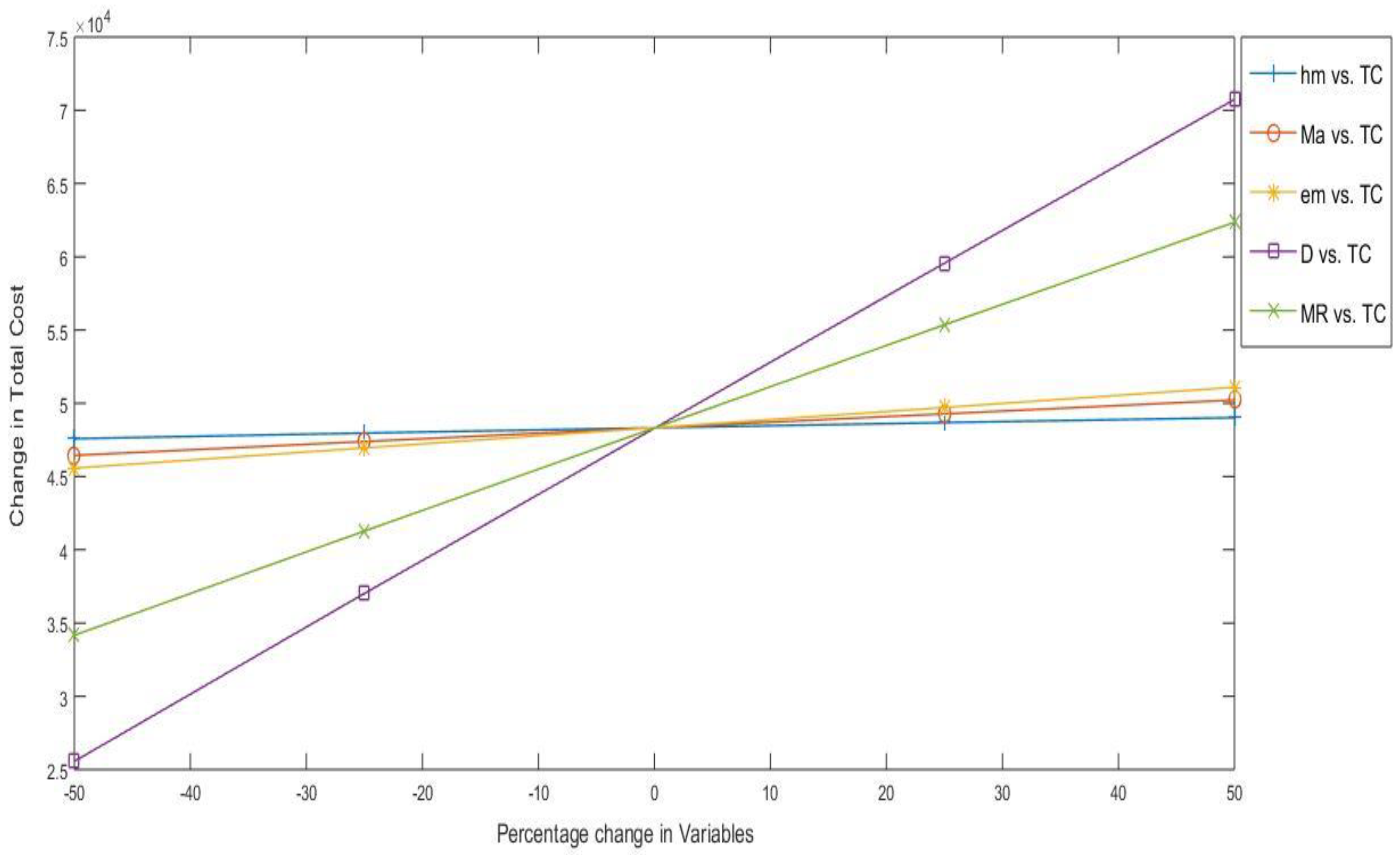
• Increase in the demand rate “D” increases the total cost TC. The total cost is more influenced by the demand rate. Changing the demand value by 50% can result in a change of 47% in the total cost.
• When the marginal cost M_R increases, it increases the TC. It is the second important metric that has a greater impact on TC. Changing the M_R by 50% will change the TC by 29%.
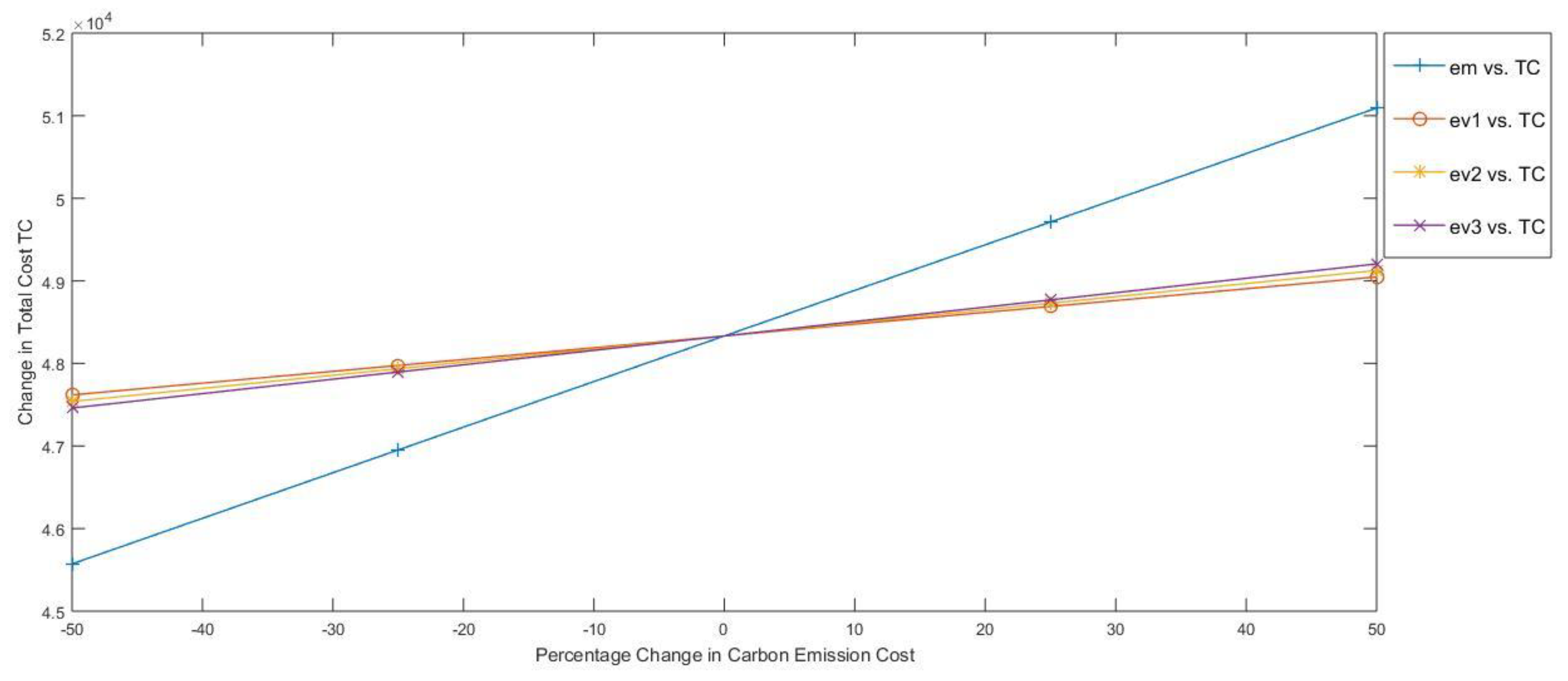
• High carbon emission will increase the total cost. It is the third biggest variable, with a TC variation of 5.7 percent.
• Increase in the manufacturing cost increases the TC. It can impact TC by 3.9% when varying by 50%.
• Inspection cost (I₁, I_2i, I₃) can cause change if there is a 3.5 % change in the TC. Holding cost of inventory (h_m, h_vi), raw material holding cost (h_r1, h_2v,i), and setup cost (s_m, s_vi) also have a direct impact on the total cost. Increasing these costs can increase the total cost (TC).
• Certain variables have zero impact on decision variables but can cause a significant effect on the total cost. These parameters are M_R, I_a, I_c, I_bi, e_m, e_bi, M_a, M_c, and M_bi.
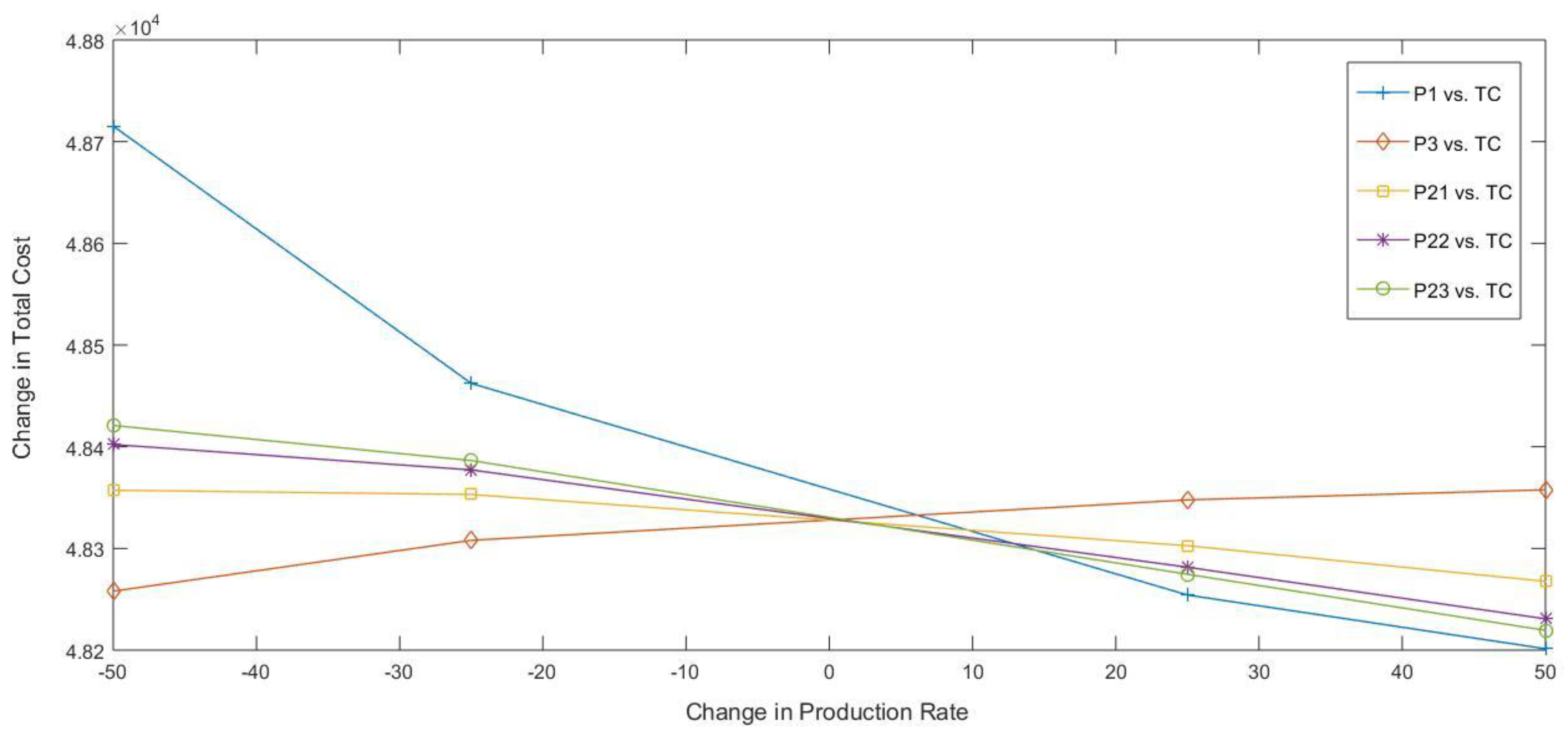
• Production rate (P₁, P_2i, and P₃) has an inverse impact on the total cost. When the production rate increases, then the total cost decreases.

The parameters that managers are worried about are those that have a significant impact on TC. The initial investment is planned to keep these variables under control. One of them is the expense of setup and carbon emissions. Reusable energy sources are used to reduce carbon emissions costs. To reduce rework costs, inline inspection should be strictly followed. To minimize rework costs, inline inspection should be followed strictly, and similarly, to minimize inspection costs, a traditional, human-based inspection can be regulated by automation and technology.

Table 6. Effect of decision variables on TC.

Iteration	Q	Q21	Q22	Q23	TC
1	30	9.413829	10.02195	10.56422	48,755.3
2	32	10.02961	10.69199	11.2784	48,600.8
3	34	10.64312	11.36237	11.99451	48,487.96
4	36	11.25424	12.0331	12.71265	48,409.84
5	38	11.86283	12.70421	13.43296	48,360.94
6 *	41.27	12.9	13.8	14.6	48,332.87
7	42	13.07191	14.04756	14.88053	48,334.14
8	44	13.67213	14.71983	15.60804	48,349.78
9	46	14.26932	15.39249	16.33818	48,381.41
10	48	14.86333	16.06557	17.0711	48,427.02
11	50	15.45406	16.73904	17.8069	48,484.95

* Optimal run to achieving the lowest TC.

shows what effect the decision variables have on the objective function TC when we change their values from the optimum value suggested by our model. It can be seen that iteration number 6 is the only optimal value of Q for the minimum TC.

The below Figure 2 shows the relation of production lot size and total cost of the supply chain.

Figure 3 depicts the graphical representation of sensitivity analysis. The graphical representation indicates that the marginal and demand lines have a higher impact on the total cost %. A minor change in one of these variables will have a significant influence on the total cost. The other variables have a slight impact on the total cost as well. Only when the marginal and demand rates are changed significantly does the total cost abruptly alter. The lines of all the other variables can be recognized through different colors and markers. The marginal rate and demand have a significant impact on output, as this graph indicates. Similarly, the third line is the carbon emission cost line, which has the third greatest impact on total cost and can affect the overall cost with a tiny modification. The manufacturing cost is the fourth item in this category, and similarly, holding cost is the next factor that has higher impact on the total cost. When the production rate increases, the total cost decreases. The sensitivity analysis for production rate is shown in Appendix C Figure A1. A separate graph of the sensitivity analysis of major parameters, such as holding cost, setup cost, and carbon emission cost, is also given in Appendix C Figure A2, Figure A3 and Figure A4.

7. Conclusions

Process outsourcing has been mathematically modelled for successful management of supply and inventory between manufacturer and multi-vendor. The total cost of supply chain is minimized with the optimization of the production quantity and outsourcing quantity. The parts are outsourced to the vendor and returned back to the manufacturer for remaining operations. The process has been modelled and optimized for effective SCM. The process outsourcing model is one of the significant contributions of the proposed research, which is important for the understanding of the managers and decision makers about the optimal production quantity and managing optimal outsourcing quantity among various vendors. An extra inventory is created at the lower end of the manufacturer, which is managed and controlled well using mathematical modelling for the smooth flow of products in SCM.

The imperfection is modelled in the proposed manufacturer and vendor-based SCM. Inspection is performed on all production and outsourcing quantities, where the defective items are reworked. The sensitivity analysis shows a dramatic relationship; i.e., the change in market demand shows a high-rise curve, the marginal rate of the vendor is also very significant for the management of the outsourcing operation in SCM, and carbon emission cost has an intermediate impact on the total cost, while other all factors have a very low impact on the total cost of SCM. The managers need to see the significant cost parameters for the management of outsourcing in SCM.

Outsourcing is a very important operation of the manufacturing firm. There are too many new research ideas and contributions available in the current field for the development of the outsourcing process in the SCM. The model can be extended by considering variable demand pattern, i.e., price or advertisement cost depending on demand, time-based demand, quality as a function of demand, etc. The deterministic model can be converted into a probabilistic one if the product’s demand follows a certain distribution function. Stochastic modelling can be utilized to reflect the real scenario of the market demand pattern as a new paradigm with process outsourcing operations in the proposed SCM. Process outsourcing was modelled in the research study; however, research can be performed to model product outsourcing. Overall, the research work is an important direction in the management of outsourcing and inventory between manufacturers and vendors for effective SCM.

References

- Kroes, J.R.; Ghosh, S. Outsourcing congruence with competitive priorities: Impact on supply chain and firm performance. J. Oper. Manag. 2009, 28, 124–143. [Google Scholar] [CrossRef]
- Bernard, K. The effect of outsourcing on supply chain performance at Cadbury Kenya Limited. Int. J. Logist. Procure. Manag. 2019, 1, 123–138. [Google Scholar]
- Hila, C.M.; Dumitraşcu, O. Outsourcing within a Supply Chain Management Framework. In Proceedings of the 8th International Management Conference, Bucharest, Romania, 6–7 November 2014. [Google Scholar]
- Kroes, J.R. Outsourcing of supply chain processes: Evaluating the impact of congruence between outsourcing drivers and competitive priorities on performance. Ga. Inst. Technol. 2007. [Google Scholar]
- Dolgui, A.; Ivanov, D.; Sokolov, B. Ripple effect in the supply chain: An analysis and recent literature. Int. J. Prod. Res. 2018, 56, 414–430. [Google Scholar] [CrossRef] [Green Version]
- Sun, J.; Tang, J.; Fu, W.; Chen, Z.; Niu, Y. Construction of a multi-echelon supply chain complex network evolution model and robustness analysis of cascading failure. Comput. Ind. Eng. 2020, 144, 106457. [Google Scholar] [CrossRef]
- Gurnani, H.; Yigal, G. Coordination in decentralized assembly systems with uncertain component yields. Eur. J. Oper. Res. 2007, 176, 1559–1576. [Google Scholar] [CrossRef]
- Li, X.; Li, Y.; Cai, X. Double marginalization and coordination in the supply chain with uncertain supply. Eur. J. Oper. Res. 2013, 226, 228–236. [Google Scholar] [CrossRef]
- Jaber, M.Y.; Zanoni, S.; Zavanella, L.E. Economic order quantity models for imperfect items with buy and repair options. Int. J. Prod. Econ. 2014, 155, 126–131. [Google Scholar] [CrossRef]
- Shaban, A.; Costantino, F.; Di Gravio, G.; Tronci, M. A new efficient collaboration model for multi-echelon supply chains. Expert Syst. Appl. 2019, 128, 54–66. [Google Scholar] [CrossRef]
- Tang, S.; Wang, W.; Zhou, G. Remanufacturing in a competitive market: A closed-loop supply chain in a Stackelberg game framework. Expert Syst. Appl. 2020, 161, 113655. [Google Scholar] [CrossRef]
- Hilletofth, P.; Hilmola, O.P. Role of logistics outsourcing on supply chain strategy and management: Survey findings from Northern Europe. Strateg. Outsourcing Int. J. 2010, 3, 46–61. [Google Scholar] [CrossRef]
- Kumar, M.; Vrat, P.; Shankar, R. A fuzzy goal programming approach for vendor selection problem in a supply chain. Comput. Ind. Eng. 2004, 46, 69–85. [Google Scholar] [CrossRef]
- Amid, A.; Ghodsypour, S.; O’Brien, C. A weighted additive fuzzy multiobjective model for the supplier selection problem under price breaks in a supply chain. Int. J. Prod. Econ. 2009, 121, 323–332. [Google Scholar] [CrossRef]
- Rezaei, J.; Davoodi, M. A deterministic, multi-item inventory model with supplier selection and imperfect quality. Appl. Math. Model. 2008, 32, 2106–2116. [Google Scholar] [CrossRef]
- Karpak, B.; Kumcu, E.; Kasuganti, R.R. Purchasing materials in the supply chain: Managing a multi-objective task. Eur. J. Purch. Supply Manag. 2001, 7, 209–216. [Google Scholar] [CrossRef]
- Scott, C.; Lundgren, H.; Thompson, P. Guide to Outsourcing in Supply Chain Management. Guide Supply Chain Manag. 2018, 2, 189–202. [Google Scholar]
- Shy, O.; Stenbacka, R. Strategic outsourcing. J. Econ. Behav. Organ. 2003, 50, 203–224. [Google Scholar] [CrossRef]
- Behara, R.S.; Gundersen, D.E.; Capozzoli, E.A. Trends in information systems outsourcing. Int. J. Purch. Mater. Manag. 1995, 31, 45–51. [Google Scholar] [CrossRef]
- Chiu, S.W.; Liu, C.J.; Li, Y.Y.; Chou, C.L. Manufacturing lot size and product distribution problem with rework, outsourcing and discontinuous inventory distribution policy. Int. J. Eng. Model. 2017, 30, 49–61. [Google Scholar]
- Jamal, A.M.M.; Sarker, B.R.; Mondal, S. Optimal manufacturing batch size with rework process at a single-stage production system. Comput. Ind. Eng. 2004, 47, 77–89. [Google Scholar] [CrossRef]
- Sarkar, B.; Cárdenas-Barrón, L.E.; Sarkar, M.; Singgih, M.L. An economic production quantity model with random defective rate, rework process and backorders for a single stage production system. J. Manuf. Syst. 2014, 33, 423–435. [Google Scholar] [CrossRef]
- Cárdenas-Barrón, L.E. Economic production quantity with rework process at a single-stage manufacturing system with planned backorders. Comput. Ind. Eng. 2009, 57, 1105–1113. [Google Scholar] [CrossRef]
- Widyadana, G.A.; Wee, H.M. An economic production quantity model for deteriorating items with multiple production setups and rework. Int. J. Prod. Econ. 2012, 138, 62–67. [Google Scholar] [CrossRef]
- Sarkar, B.; Sana, S.S.; Chaudhuri, K. An imperfect production process for time varying demand with inflation and time value of money—An EMQ model. Expert Syst. Appl. 2011, 38, 13543–13548. [Google Scholar] [CrossRef]
- Taleizadeh, A.A.; Sari-Khanbaglo, M.P.; Cárdenas-Barrón, L.E. Outsourcing rework of imperfect items in the economic production quantity (EPQ) inventory model with backordered demand. IEEE Trans. Syst. Man Cybern. Syst. 2017, 49, 2688–2699. [Google Scholar] [CrossRef]
- Alvarez, L.H.; Stenbacka, R. Partial outsourcing: A real options perspective. Int. J. Ind. Organ. 2007, 25, 91–102. [Google Scholar] [CrossRef]
- Benaroch, M.; Webster, S.; Kazaz, B. Impact of sourcing flexibility on the outsourcing of services under demand uncertainty. Eur. J. Oper. Res. 2012, 219, 272–283. [Google Scholar] [CrossRef]
- Inderfurth, K.; Kelle, P. Capacity reservation under spot market price uncertainty. Int. J. Prod. Econ. 2011, 133, 272–279. [Google Scholar] [CrossRef]
- Spinler, S.; Huchzermeier, A. The valuation of options on capacity with cost and demand uncertainty. Eur. J. Oper. Res. 2006, 171, 915–934. [Google Scholar] [CrossRef]
- Liu, Z.; Nagurney, A. Supply chain networks with global outsourcing and quick response production under demand and cost uncertainty. Ann. Oper. Res 2013, 208, 251–289. [Google Scholar] [CrossRef]
- Nosoohi, I.; Nookabadi, A.S. Outsource planning through option contracts with demand and cost uncertainty. Eur. J. Oper. Res. 2016, 250, 131–142. [Google Scholar] [CrossRef]
- Chen, K.; Xiao, T. Outsourcing strategy and production disruption of supply chain with demand and capacity allocation uncertainties. Int. J. Prod. Econ. 2015, 170, 243–257. [Google Scholar] [CrossRef]
- Zhao, L.; Langendoen, F.R.; Fransoo, J.C. Supply management of high-value components with a credit constraint. Flex. Serv. Manuf. J. 2012, 24, 100–118. [Google Scholar] [CrossRef] [Green Version]
- Min, H. Examining logistics outsourcing practices in the United States: From the perspectives of third-party logistics service users. Logist. Res. 2013, 6, 133–144. [Google Scholar] [CrossRef]
- Lacity, M.C.; Khan, S.A.; Yan, A. Review of the empirical business services sourcing literature: An update and future directions. J. Inf. Technol. 2016, 31, 269–328. [Google Scholar] [CrossRef]
- Qin, L.; Wu, H.; Zhang, N.; Li, X. Risk identification and conduction model for financial institution IT outsourcing in China. Inf. Technol. Manag. 2012, 13, 429–444. [Google Scholar] [CrossRef]
- Oh, W.; Gallivan, M.J.; Kim, J.W. The market’s perception of the transactional risks of information technology outsourcing announcements. J. Manag. Inf. Syst. 2006, 22, 271–303. [Google Scholar] [CrossRef]
- Earl, M.J. The risks of outsourcing IT. Sloan Manag. Rev. 1996, 37, 26–32. [Google Scholar]
- Gewald, H.; Dibbern, J. Risks and benefits of business process outsourcing: A study of transaction services in the German banking industry. Inf. Manag. 2009, 46, 249–257. [Google Scholar] [CrossRef]
- Choi, T.; Wallace, S.W.; Wang, Y. Risk management and coordination in service supply chains: Information, logistics, and outsourcing. J. Oper. Res. Soc. 2016, 67, 159–164. [Google Scholar] [CrossRef]
- Tsai, M.; Lai, K.; Lloyd, A.E.; Lin, H. The dark side of logistics outsourcing—unraveling the potential risks leading to failed relationships. Transp. Res. Part E Logist. Transp. Rev. 2012, 48, 178–189. [Google Scholar] [CrossRef]
- Wang, Y.; Wallace, S.W.; Shen, B.; Choi, T. Service supply chain management: A review of operational models. Eur. J. Oper. Res. 2015, 247, 685–698. [Google Scholar] [CrossRef]
- Chen, J.; Liang, L.; Yao, D.Q. Factory encroachment and channel selection in an outsourced supply chain. Int. J. Prod. Econ. 2018, 215, 73–83. [Google Scholar] [CrossRef]
- Akan, M.; Ata, B.; Lariviere, M.A. Asymmetric Information and Economies of Scale in Service Contracting. Manuf. Serv. Oper. Manag. 2011, 13, 58–72. [Google Scholar] [CrossRef] [Green Version]
- Xin, Y.; Huang, R.; Song, M.; Mishra, N. Pre-positioning inventory and service outsourcing of relief material supply chain. Int. J. Prod. Res. 2018, 56, 6859–6871. [Google Scholar]
- Wu, J.; Wang, H.; Shang, J. Multi-sourcing and information sharing under competition and supply uncertainty. Eur. J. Oper. Res. 2019, 278, 658–671. [Google Scholar] [CrossRef]
- Li, X.; Li, Y.; Cai, X.; Shan, J. Service channel choice for supply chain: Who is better off by undertaking the service? Prod. Oper. Manag. 2016, 25, 516–534. [Google Scholar] [CrossRef]
- Huang, M.; Tu, J.; Chao, X.; Jin, D. Quality risk in logistics outsourcing: A fourth party logistics perspective. Eur. J. Oper. Res. 2019, 276, 855–879. [Google Scholar] [CrossRef]
- Zhang, S.; Zhang, J.; Zhu, G. Retail service investing: An anti-encroachment strategy in a retailer-led supply chain. Omega 2019, 84, 212–231. [Google Scholar] [CrossRef]
- Yue, J.; Ryan, J.K. Price and service competition in an outsourced supply chain. Prod. Oper. Manag. 2012, 21, 331–344. [Google Scholar]
- Ching, W.K.; Choi, S.M.; Huang, X. Inducing high service capacities in outsourcing via penalty and competition. Int. J. Prod. Res. 2011, 49, 5169–5182. [Google Scholar] [CrossRef]
- Ding, H.; Chen, X.; Lin, K.; Wei, Y. Collaborative mechanism of project profit allotment in petroleum engineering service chain with customized integration. Int. J. Prod. Econ. 2019, 214, 163–174. [Google Scholar] [CrossRef]
Figure 1.
Inventory diagram of the supply chain management considering process outsourcing.
Figure 2.
Total cost TC with respect to production lot size Q.
Figure 3.
Graphical representation of sensitivity analysis.