Topology Adaptive Graph Estimation in High Dimensions

Abstract

We introduce Graphical TREX (GTREX), a novel method for graph estimation in high-dimensional Gaussian graphical models. By conducting neighborhood selection with TREX, GTREX avoids tuning parameters and is adaptive to the graph topology. We compared GTREX with standard methods on a new simulation setup that was designed to assess accurately the strengths and shortcomings of different methods. These simulations showed that a neighborhood selection scheme based on Lasso and an optimal (in practice unknown) tuning parameter outperformed other standard methods over a large spectrum of scenarios. Moreover, we show that GTREX can rival this scheme and, therefore, can provide competitive graph estimation without the need for tuning parameter calibration.

1. Introduction

Graphical models have become an important tool to find and describe patterns in high-dimensional data ([1], Chapter 3). In biology, for example, graphical models have been successfully applied to estimate interactions between genes from high-throughput expression profiles [2,3], to predict contacts between protein residues from multiple sequence alignments [4], and to uncover the interactions of microbes from gene sequencing data [5]. Graphical models represent the conditional dependence structure of the underlying random variables as a graph. Learning a graphical model from data requires a simultaneous estimation of the graph and of the probability distribution that factorizes according to this graph. In the Gaussian case, it is well known that the underlying graph is determined by the non-zero entries of the precision matrix (the inverse of the population covariance matrix). Gaussian graphical models have become particularly popular after the advent of computationally efficient approaches, such as neighborhood selection [6] and sparse covariance estimation [7,8], which can learn even high-dimensional graphical models. Neighborhood selection, on the one hand, reconstructs the graph by estimating the local neighborhood of each node via Lasso [9]. This approach is usually seen as a proxy to the covariance selection problem [10]. On the other hand, References [7,8] showed that the graph and the precision matrix can be simultaneously estimated by solving a global optimization problem. State-of-the-art solvers are graphical Lasso [10] and the Quadratic Approximation of Inverse Covariance (QUIC) method [11]. Both approaches can be extended beyond the framework of Gaussian graphical models. To mention two of the many examples, Reference [12] studied neighborhood selection for Ising models, and [13] introduced a semi-parametric penalized likelihood estimator that allows for non-Gaussian distributions of the data.

Although the field has advanced tremendously in the past decade, there are still a number of challenges, both from a practical and a theoretical point of view. First, the conditions that are currently imposed [6,12,14,15] to show consistency in graph and/or graphical model estimation are difficult to meet or verify in practice. Moreover, the performance of any of the standard methods heavily depends on the simulation setup or the data at hand [5,16,17]. Furthermore, standard neighborhood selection and covariance estimation methods require a careful calibration of a tuning parameter, especially because the model complexity is known a priori only in very few examples [4]. In practice, the tuning parameters are calibrated via cross-validation, classical information criteria such as the AIC and BIC [8], or stability criteria [18]. However, different calibration schemes can result in largely disparate estimates [18].

To approach some of the practical challenges, we introduce Graphical TREX (GTREX), a novel method for graph estimation based on neighborhood selection with TREX [19]. The main feature of GTREX is that it can make tuning parameters superfluous, which renders this method particularly useful in practice. We also introduce a novel simulation setup that may serve as a benchmark to assess the strengths and shortcomings of different methods.

Our simulations showed that, if the tuning parameter is optimally chosen, standard neighborhood selection with the “or-rule” outmatches other standard methods across a wide range of scenarios. Our simulations also showed that GTREX can rival this method in many scenarios. Since optimal tuning parameters depend on unknown quantities and, therefore, are not accessible in practice, this demonstrates that GTREX is a promising alternative for graph estimation in high-dimensional graphical models.

The remainder of the paper is structured as follows. After specifying the framework and notation, we introduce GTREX in Section 2. We then describe the experimental scenarios in Section 3 and present the numerical results in Section 4. We finally conclude in Section 5.

Framework and Notation

We considered n samples from a p-dimensional Gaussian distribution ${\mathcal{N}}_p(0,\Sigma )$ with positive-definite, symmetric covariance matrix $\Sigma \in {\mathbb{R}}^{p\times p}$. The samples are summarized in the matrix $X\in {\mathbb{R}}^{n\times p}$ such that $X_{ij}$ corresponds to the jth component of the ith sample. We call ${\Sigma }^{-1}$ the precision matrix and note that the precision matrix is symmetric.

The Gaussian distribution ${\mathcal{N}}_p(0,\Sigma )$ can be associated with an undirected graph $\mathcal{G}=(\mathcal{V},\mathcal{E})$, where $\mathcal{V}=\{1,\dots ,p\}$ is the set of nodes and $\mathcal{E}=\mathcal{V}\times \mathcal{V}$ the set of (undirected) edges that consists of all pairs $(i,j),(j,i)\in \mathcal{V}\times \mathcal{V}$ that fulfill $i\ne j$ and ${({\Sigma }^{-1})}_{ij}\ne 0$. We denote by $e_{ij}$ (and equivalently by $e_{ji}$) the edge that corresponds to the pair $(i,j),(j,i)$ and by $s:=\left|\mathcal{E}\right|$ the total number of edges in the graph $\mathcal{G}$.

We denote by $supp(\beta )$ the support of a vector $\beta$, by $a\vee b$ and $a\wedge b$ the maximum and minimum, respectively, of two constants $a,b\in \mathbb{R}$, and by $|·|$ the cardinality of a set.

In this paper, we focused on estimating which entries of the precision matrix ${\Sigma }^{-1}$ are non-zero from the data X. This is equivalent to estimating the set of edges $\mathcal{E}$ from X. We assessed the quality of an estimate $\tilde{\mathcal{E}}$ via the Hamming distance to the true set of edges $\mathcal{E}$ given by $d_H(\tilde{\mathcal{E}},\mathcal{E}):=|\{e_{ij}:e_{ij}\in \tilde{\mathcal{E}},e_{ij}\notin \mathcal{E}\}\cup \{e_{ij}:e_{ij}\notin \tilde{\mathcal{E}},e_{ij}\in \mathcal{E}\}|$.

2. Methodology

Before introducing our new estimator GTREX, we first recall the definitions of graphical Lasso and of neighborhood selection with Lasso. For a fixed tuning parameter $\lambda >0$, Graphical Lasso (GLasso) estimates the precision matrix ${\Sigma }^{-1}$ from X according to: [10]

$${\widehat{\Theta }}_{\mathrm{GLasso}}^{\lambda }\in argmin\left\{-logdet(\Theta )+trace(\widehat{\Sigma }\Theta )+\lambda {\parallel \Theta \parallel }_1\right\},$$

where the minimum is taken over all positive-definite matrices $\Theta \in {\mathbb{R}}^{p\times p}$, $\widehat{\Sigma }:=X^{\top }X/n$ is the sample covariance matrix, and ${\parallel \Theta \parallel }_1:={\sum }_{i,j=1}^p\left|{\Theta }_{ij}\right|$ is the sum of the entries of $\Theta$. The corresponding estimator for the set of edges $\mathcal{E}$ is then:

$${\widehat{\mathcal{E}}}_{\mathrm{GLasso}}^{\lambda }:=\{e_{ij}:|{({\widehat{\Theta }}_{\mathrm{GLasso}}^{\lambda })}_{ij}|>0\}.$$

(1)

This defines a family of graph estimators indexed by the tuning parameter $\lambda$. To assess the potential of GLasso, we define ${\widehat{\mathcal{E}}}_{\mathrm{GLasso}}^{*}:={\widehat{\mathcal{E}}}_{\mathrm{GLasso}}^{{\lambda }^{*}}$, where ${\lambda }^{*}$ is the tuning parameter that minimizes the Hamming distance to the true edge set $\mathcal{E}$. We stress, however, that the optimal tuning parameter ${\lambda }^{*}$ is not accessible in practice and that there are no guarantees that standard calibration schemes provide a tuning parameter close to ${\lambda }^{*}$. Therefore, the performance of ${\widehat{\mathcal{E}}}_{\mathrm{GLasso}}^{*}$ is to be understood as an upper bound for the performance of GLasso.

Besides GLasso, we also considered neighborhood selection with Lasso. To this end, we define for any matrix $\overline{X}\in {\mathbb{R}}^{n^{\prime }\times p}$, $n^{\prime }\le n$, and for any node $k\in \mathcal{V}$, the vector ${\overline{X}}^k\in {\mathbb{R}}^{n^{\prime }}$ as the kth column of $\overline{X}$ and the matrix ${\overline{X}}^{-k}\in {\mathbb{R}}^{n^{\prime }\times (p-1)}$ as $\overline{X}$ without the kth column. For a fixed tuning parameter $\lambda >0$, the estimates of Lasso for node k are defined according to [9]:

$$\widehat{\beta }{}_{\mathrm{LASSO}}^{\lambda }(k;X)\in \underset{\begin{array}{c}\beta \in {\mathbb{R}}^p\\ {\beta }_k=0\end{array}}{argmin}\left\{\parallel X^k{-X\beta \parallel }_2^2+\lambda {\parallel \beta \parallel }_1\right\}.$$

(2)

The corresponding set of edges ${\widehat{\mathcal{E}}}_{\mathrm{and}}^{\lambda }$ (with the “and-rule”) and ${\widehat{\mathcal{E}}}_{\mathrm{or}}^{\lambda }$ (with the “or-rule”) are then defined via Algorithm 1 following Meinshausen and Bühlmann [6]. (An interesting alternative would be the symmetric approach in [20].) Similarly as above, we define the optimal representative (in terms of the Hamming distance) of these families of estimators as ${\widehat{\mathcal{E}}}_{\mathrm{and}}^{*}$, called MB(and), and ${\widehat{\mathcal{E}}}_{\mathrm{or}}^{*}$, called MB(or). Again, in practice, it is not known which tuning parameters are optimal; however, MB(and) and MB(or) can highlight the potential of neighborhood selection with Lasso.   

Algorithm 1:Neighborhood selection with Lasso.

Data: $X\in {\mathbb{R}}^{n\times p}$, $\lambda >0$;  Result: ${\widehat{\mathcal{E}}}_{\mathrm{and}}^{\lambda }$, ${\widehat{\mathcal{E}}}_{\mathrm{or}}^{\lambda }$;  Initialize a matrix $C:=0_{p\times p}$;  for $k=1$ to p do$\phantom{(}$   Compute $\widehat{\beta }{}_{\mathrm{LASSO}}^{\lambda }(k;X)$ according to (2);   Update the kth column $C^k$ of the matrix C         according to $C^k:=\widehat{\beta }{}_{\mathrm{LASSO}}^{\lambda }(k;X)$;  end$\phantom{(}$  Set the estimated sets to   ${\widehat{\mathcal{E}}}_{\mathrm{and}}^{\lambda }:=\{e_{ij}:|C_{ij}|\vee |C_{ji}|>0\}$ and   ${\widehat{\mathcal{E}}}_{\mathrm{or}}^{\lambda }:=\{e_{ij}:|C_{ij}|\wedge |C_{ji}|>0\}$;

We finally introduce Graphical TREX (GTREX). To this end, we considered TREX for node k on a subsample $\overline{X}$ according to [19]:

$$\widehat{\beta }(k;\overline{X})\in \underset{\begin{array}{c}\beta \in {\mathbb{R}}^p\\ {\beta }_k=0\end{array}}{argmin}\left\{\frac{\parallel {\overline{X}}^k-\overline{X}{\beta \parallel }_2^2}{\parallel {({\overline{X}}^{-k})}^{\top }({\overline{X}}^k-\overline{X}\beta ){\parallel }_{\infty }}+{\parallel \beta \parallel }_1\right\}.$$

(3)

For a fixed number of bootstraps $b\in \{1,2,\dots \}$ and threshold $t\ge 0$, we then define GTREX as the set of edges $\widehat{\mathcal{E}}$ provided by Algorithm 2. The bootstrap part of the algorithm might remind us of the stability selection method [21], but has a different focus: it concerns the edge selection directly rather than the calibration of a tuning parameter.

For the actual implementation, we followed [19] and invoked that ${\parallel a\parallel }_{\infty }\approx {\parallel a\parallel }_q$ for q sufficiently large. We then used a projected sub-gradient method to minimize the objective:

$$\underset{\begin{array}{c}\beta \in {\mathbb{R}}^p\\ {\beta }_k=0\end{array}}{min}\left\{\frac{\parallel {\overline{X}}^k-\overline{X}{\beta \parallel }_2^2}{\parallel {({\overline{X}}^{-k})}^{\top }({\overline{X}}^k-\overline{X}\beta ){\parallel }_q}+{\parallel \beta \parallel }_1\right\},$$

(4)

which corresponds to (3).   

Algorithm 2: GTREX.

Data: $X\in {\mathbb{R}}^{n\times p}$, $b\in \{1,2,\dots \}$, $t\in [0,1]$;  Result: $\widehat{\mathcal{E}}$, $F\in {\mathbb{R}}^{p\times p}$;  Initialize all frequencies $F:=0_{p\times p}$;  for $k=1$ to p do    for $l=1$ to b do      Generate sequential bootstrap sample $\overline{X}$ of X;      Compute $\widehat{\beta }(k;\overline{X})$ according to (3);      Update the frequencies for the edges adjacent        to node k        for $m=1$ to p do          if $m\in supp(\widehat{\beta }(k;\overline{X}))$ then            $F_{km}:=F_{km}+\frac{1}{b}$;          end        end    end  end  Set the estimated set of edges to    $\widehat{\mathcal{E}}:=\{e_{ij}:F_{ij}\vee F_{ji}>t\}$;

3. Experimental Scenarios

Besides the number of parameters p, the sample size n, and the level of sparsity of the graph, the graph topology can have a considerable impact on the performance of the different methods [15]. For example, standard estimators require many samples for graphs with many hub nodes (nodes that are connected to many other nodes). Reference [15] presented a number of toy examples that confirmed these theoretical predictions. The following experimental setup was motivated by these insights. We considered six different graph topologies with varying hub structures, ranging from a single-hub case to Erdos–Rényi graphs:

• Single-hub graph:
  The set of edges is first set to $\mathcal{E}=\{e_{1j}:j\in \{2,\dots ,p\}\}$. Until the number of edges s is exhausted, edges are then uniformly at random added to $\mathcal{E}$;
• Double-hub graph
  The set of edges is first set to $\mathcal{E}=\{e_{1j}:j\in \{2,\dots ,p/2\}\}\cup \{e_{(p/2+1)j}:j\in \{p/2+2,\dots ,p\}\}$. Until the number of edges s is exhausted, edges are then uniformly at random added to $\mathcal{E}$;
• Four-hub graph
  The set of edges is first set to $\mathcal{E}=\left\{e_{1j}:j\in \{2,\dots ,p/4\}\right\}\cup \{e_{(p/4+1)j}:j\in \{p/4+2,\dots ,p/2\}\}\cup \{e_{(p/2+1)j}:j\in \{p/2+2,\dots ,3p/4\}\}\cup \{e_{(3p/4+1)j}:j\in \{3p/4+2,\dots ,p\}\}$. Until the number of edges s is exhausted, edges are then uniformly at random added to $\mathcal{E}$;
• Four-niche graph:
  Within each set of nodes $\{1,\dots ,p/4\}$, $\{p/4+1,\dots ,2p/4\}$, $\{2p/4+1,\dots ,3p/4\}$, $p/4-1$ edges are uniformly selected at random and added to the set of edges. Until the number of edges s is exhausted, edges (connecting any nodes of the entire graph) are then uniformly at random added to $\mathcal{E}$;
• Erdos–Rényi graph:
  Until the number of edges s is exhausted, edges are uniformly at random added to $\mathcal{E}$;
• Scale-free graph:
  First, a set of edges is constructed with the preferential attachment algorithm [22]: The set of edges is first set to $\mathcal{E}=\{e_{12}\}$. For each node $i\in \mathcal{V}\backslash \{1,2\}$, an edge $e_{ij}$ is then iteratively added to $\mathcal{E}$ until the number of edges s is exhausted. The probability of selecting the edge $e_{ij}$ is set proportional to the degree of node $j\in \mathcal{V}$ (that is, the number of edges at node j) in the current set of edges. One could also change this probability; for example, one could weight the degree more heavily, that is put more emphasis on nodes that already have edges connected to them. In general, the more weight on the degree, the more the graphs look the same as hub graphs and, therefore, the better the performance of our method relative to GLasso and MB.

Given a graph $\mathcal{G}$ that consists of a set of nodes $\mathcal{V}$ and a set of edges $\mathcal{E}$ as described above, a precision matrix ${\Sigma }^{-1}$ is generated as follows: The set of edges $\mathcal{E}$ determines which off-diagonal entries of the precision matrix ${\Sigma }^{-1}$ are non-zero. The values of these entries are independently sampled uniformly at random in $[-a_{max},-a_{min}]\cup [a_{min},a_{max}]$ for some $a_{max}>a_{min}>0$. The diagonal entries of ${\Sigma }^{-1}$ are then set to a common value, which is chosen to ensure a given condition number $cond:=cond({\Sigma }^{-1})$ (the ratio of the largest eigenvalue to the smallest eigenvalue of ${\Sigma }^{-1}$).

4. Numerical Results

We performed all numerical computations in MATLAB 2014a on a standard MacBook Pro with a 2.8 GHz Dual-core Intel i7 and 16 GB 1600 MHz DDR3 memory. To compute the GLasso paths, we used the C implementation of the QUIC algorithm and the corresponding MATLAB wrapper [11]. We set the maximum number of iterations to 200, which ensured the global convergence of the algorithm in our settings. To compute the Lasso paths for the neighborhood selection schemes, we used the MATLAB internal procedure lasso.m, which follows the popular glmnet R code. We implemented a neighborhood selection wrapper mblasso.m that returns the graph traces over the entire path for the “and-rule” and the “or-rule.” Both for GLasso and neighborhood selection, we used a fine grid of step size $0.01$ on the unit interval for the tuning parameter $\lambda$, resulting in a path over 100 values of $\lambda$. To compute TREX, we optimized the approximate TREX objective function with $q=40$ using Schmidt’s PSS algorithm implemented in L1General2_PSSgb.m. We used the PSS algorithm with the standard parameter settings and set the initial solution to the parsimonious all-zeros vector ${\beta }_{\mathrm{init}}={(0,\dots ,0)}^{\top }\in {\mathbb{R}}^p$. We used the following PSS stopping criteria: minimum relative progress tolerance optTol = 1 × 10⁻⁷, minimum gradient tolerance progTol = 1 × 10⁻⁹, and maximum number of iterations $\mathrm{maxIter}=0.2p$. We implemented a wrapper gtrex.m that integrates the nodewise TREX solutions and returns the frequency table for each edge and the resulting graph estimate. We used $b=31$ bootstrap samples in B-TREX; increasing the number of bootstraps did not result in significant changes of the GTREX solutions.

We generated the graphical models as outlined in Section 3. We set the number of nodes to $p\in \{100,200\}$, the number of edges to $s=p-1$, the bounds for the absolute values of the off-diagonal entries of the precision matrix to $a_{min}=0.2$ and $a_{max}=1$, and the condition number to $cond=100$. We then drew $n\in \{p,2p,4p,10p\}$ samples from the resulting normal distribution and normalized each sample to have the Euclidean norm equal to $\sqrt{n}$. We measured the performance of the estimators in terms of the Hamming distance to the true graph and in terms of the Precision/Recall. We stress that for GLasso, MB(or), and MB(and), we selected the (in practice unknown) tuning parameter $\lambda$ that minimizes the Hamming distance to the true graph. For GTREX, we set the frequency threshold to $t=0.75$; however, it turned out that GTREX is robust with respect to the choice of the threshold. For each graph, we report the averaged results over 20 repetitions.

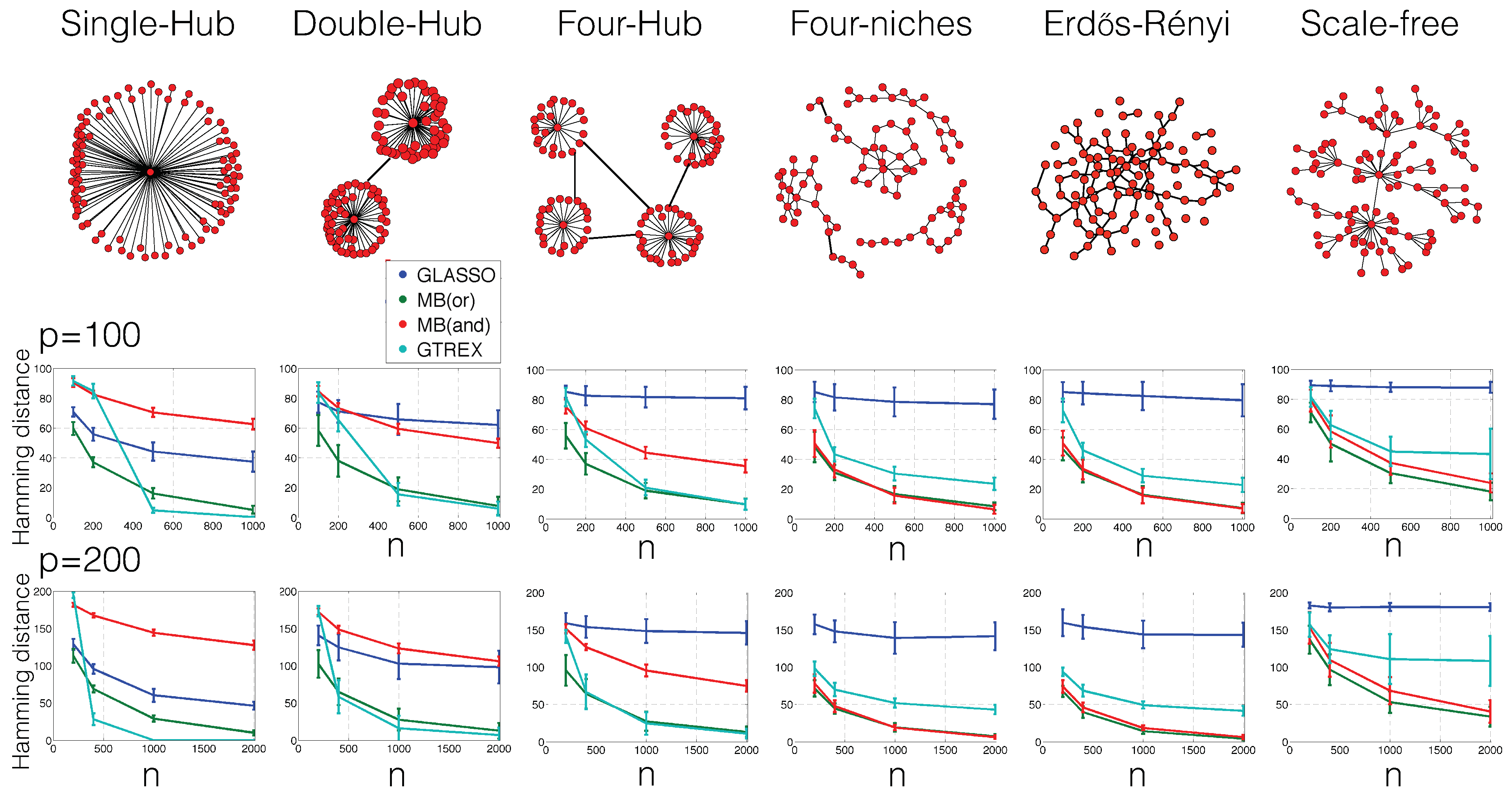
The results are summarized in Figure 1 and in

Table 1. Precision and Recall for the single-hub graph with $a_{min}=0.2$, $a_{max}=1$, $s=p-1$, and $cond=100$.

$\mathit{n}=100$, $\mathit{p}=100$
Method	P	R
GLasso	0.99	0.35
MB(or)	0.99	0.48
MB(and)	0.99	0.49
GTREX	0.99	0.13
$n=500$, $p=100$
Method	P	R
GLasso	0.99	0.59
MB(or)	0.99	0.87
MB(and)	0.99	0.92
GTREX	1.00	0.99
$n=200$, $p=200$
Method	P	R
GLasso	1.00	0.25
MB(or)	1.00	0.30
MB(and)	1.00	0.29
GTREX	0.99	0.05
$n=1000$, $p=200$
Method	P	R
GLasso	1.00	0.44
MB(or)	1.00	0.58
MB(and)	1.00	0.59
GTREX	1.00	0.60

,

Table 2. Precision and Recall for the four-hub graph with $a_{min}=0.2$, $a_{max}=1$, $s=p-1$, and $cond=100$.

$\mathit{n}=100$, $\mathit{p}=100$
Method	P	R
GLasso	1.00	0.17
MB(or)	1.00	0.55
MB(and)	0.99	0.59
GTREX	0.99	0.26
$n=500$, $p=100$
Method	P	R
GLasso	0.99	0.19
MB(or)	1.00	0.86
MB(and)	1.00	0.93
GTREX	1.00	0.80
$n=200$, $p=200$
Method	P	R
GLasso	1.00	0.15
MB(or)	1.00	0.36
MB(and)	1.00	0.40
GTREX	1.00	0.20
$n=1000$, $p=200$
Method	P	R
GLasso	0.99	0.17
MB(or)	1.00	0.54
MB(and)	1.00	0.57
GTREX	1.00	0.53

and

Table 3. Precision and Recall for the Erdos–Rényi graph with $a_{min}=0.2$, $a_{max}=1$, $s=p-1$, and $cond=100$.

$\mathit{n}=100$, $\mathit{p}=100$
Method	P	R
GLasso	1.00	0.31
MB(or)	1.00	0.61
MB(and)	0.99	0.69
GTREX	0.99	0.36
$n=500$, $p=100$
Method	P	R
GLasso	0.99	0.42
MB(or)	1.00	0.89
MB(and)	1.00	0.94
GTREX	1.00	0.71
$n=200$, $p=200$
Method	P	R
GLasso	1.00	0.30
MB(or)	1.00	0.43
MB(and)	1.00	0.46
GTREX	1.00	0.34
$n=1000$, $p=200$
Method	P	R
GLasso	0.99	0.42
MB(or)	1.00	0.57
MB(and)	1.00	0.58
GTREX	1.00	0.45

. The results with respect to the Hamming distance in Figure 1 provide three interesting insights: First, GLasso performed poorly in the Hamming distance for all considered scenarios. We suspect that this is connected with the chosen value for the condition of the precision matrix. Second, we observed marked differences between MB(and) and MB(or). In particular, the two methods had a similar performance in the scenarios with the four-niche and the Erdös–Rényi graphs, but a completely different performance in the scenarios with the hub graphs. Third, GTREX performed excellently for the hub graphs if the sample size was sufficiently large ($n>2p$) and reasonably in all other scenarios. The results with respect to Precision/Recall in Table 1, Table 2 and Table 3 show that all methods had an excellent Precision (all values were close to 1), but differed in Recall. MB(and) provided the best overall performance, but note once more that it was calibrated with the optimal tuning parameter, which is unknown in practice. GTREX was competitive in most scenarios once the sample size n was sufficiently large, which indicates that the GTREX requires a minimal number of samples to “autotune” itself to the data.

We also note that neither GTREX nor its competitors worked reasonably well when $p\gg n$ in our simulation framework. In general, we recommend using graphical modeling with care when p is larger than n.

TREX does not contain a tuning parameter, but one can argue that the frequency threshold t could be adapted to the model or the data and, therefore, plays the role of a tuning parameter in GTREX. However, the above results demonstrate that the universal value $t=0.75$ works for a large variety of scenarios. Moreover, GTREX is robust with respect to the choice of t. This is illustrated in Figure 2, where for two scenarios, we report the Hamming distances of GTREX to the true graphs as a function of t. We observed that the Hamming distances were similar over wide ranges of t. In the same figure, we also report the Hamming distances of the standard methods to the true graphs as a function of the tuning parameter $\lambda$. We see that these paths have narrow peaks, which suggests that the tuning parameters of GLasso and of neighborhood selection with Lasso need to be carefully calibrated.

Note that the results especially of Figure 1, including the tuning of the standard methods, were based on the Hamming distance as a measure of accuracy. We chose the Hamming distance, because it is a very general and widely accepted measure and, most importantly, readily comparable across different setups. However, different measures of accuracy could give different results, for example in terms of how the false estimates split into false positives and false negatives.

Note finally that there has been recent progress in the computational aspects of TREX. Reference [23] introduced a new algorithm that is guaranteed to converge to a global optimum (even though it is a non-convex problem) and requires solving at most p reasonably simple subproblems. Reference [24] developed this idea further in the context of prospective functions. In any case, the computational costs of GTREX are $\left|\mathcal{V}\right|\times b\times (\cos \mathrm{ts}\mathrm{of}\mathrm{solving}\mathrm{Equation}(3))$. In our current non-convex implementation, solving Equation (3) took about a second; in a convex implementation, it took about half a second—cf. ([23], Figure 3), and ([24], Figure 1). Hence, estimating a graph in our current simulations took about one hour on a single CPU (of course, the algorithm can be parallelized very easily).

5. Conclusions

We introduced a new method for graph estimation in high-dimensional graphical models. Unlike any other method, our estimator avoided the tuning parameter, which is usually part of the regularizer. Beyond establishing the mere fact that this is possible to begin with, we made two main contributions: First, since the method rivals standard methods even if they are calibrated with an optimal, in practice unknown tuning parameter, our paper can directly lead to more accurate estimation in practice.

Second, deriving statistical theory for tuning parameter calibration has turned out to be very difficult in all parts of high-dimensional statistics. Recent developments focused mainly on linear and logistic regression [25,26]. For graphical modeling, standard estimators are currently not equipped with a rigorously justified tuning scheme. We have not established a statistical theory for GTREX yet, but it has been shown recently that the TREX idea can provide new ways to establish such a theory [27]. Hence, we hope that our approach can indeed be complemented with comprehensive statistical theories in future research, thereby furthering the mathematical understanding of graphical modeling in general.

References

- Lederer, J. Fundamentals of High-Dimensional Statistics: With Exercises and R Labs; Springer Texts in Statistics: Heidelberg, Germany, 2022. [Google Scholar]
- Wille, A.; Zimmermann, P.; Vranová, E.; Fürholz, A.; Laule, O.; Bleuler, S.; Hennig, L.; Prelić, A.; von Rohr, P.; Thiele, L.; et al. Sparse graphical Gaussian modeling of the isoprenoid gene network in Arabidopsis thaliana. Genome Biol. 2004, 5, R92. [Google Scholar] [CrossRef] [Green Version]
- Friedman, N. Inferring Cellular Networks Using Probabilistic Graphical Models. Science 2004, 303, 799–805. [Google Scholar] [CrossRef]
- Jones, D.; Buchan, D.; Cozzetto, D.; Pontil, M. PSICOV: Precise structural contact prediction using sparse inverse covariance estimation on large multiple sequence alignments. Bioinformatics 2012, 28, 184–190. [Google Scholar] [CrossRef] [Green Version]
- Kurtz, Z.; Müller, C.; Miraldi, E.; Littman, D.; Blaser, M.; Bonneau, R. Sparse and Compositionally Robust Inference of Microbial Ecological Networks. arXiv 2014, arXiv:1408.4158. [Google Scholar] [CrossRef] [Green Version]
- Meinshausen, N.; Bühlmann, P. High Dimensional Graphs and Variable Selection with the Lasso. Ann. Stat. 2006, 34, 1436–1462. [Google Scholar] [CrossRef] [Green Version]
- Banerjee, O.; El Ghaoui, L.; D’Aspremont, A. Model selection through sparse maximum likelihood estimation for multivariate gaussian or binary data. J. Mach. Learn. Res. 2008, 9, 485–516. [Google Scholar]
- Yuan, M.; Lin, Y. Model selection and estimation in the Gaussian graphical model. Biometrika 2007, 94, 19–35. [Google Scholar] [CrossRef] [Green Version]
- Tibshirani, R. Regression shrinkage and selection via the lasso. J. R. Stat. Soc. 1996, 58, 267–288. [Google Scholar] [CrossRef]
- Friedman, J.; Hastie, T.; Tibshirani, R. Sparse inverse covariance estimation with the graphical lasso. Biostatistics 2008, 9, 432–441. [Google Scholar] [CrossRef] [Green Version]
- Hsieh, C.J.; Sustik, M.; Dhillon, I.; Ravkiumar, P. Sparse inverse covariance matrix estimation using quadratic approximation. NIPS 2011, 24, 1–18. [Google Scholar]
- Ravikumar, P.; Wainwright, M.; Lafferty, J. High-dimensional Ising model selection using L1-regularized logistic regression. Ann. Stat. 2010, 38, 1287–1319. [Google Scholar] [CrossRef] [Green Version]
- Liu, H.; Lafferty, J.; Wasserman, L. The Nonparanormal: Semiparametric Estimation of High Dimensional Undirected Graphs. J. Mach. Learn. Res. 2009, 10, 2295–2328. [Google Scholar]
- Lam, C.; Fan, J. Sparsistency and Rates of Convergence in Large Covariance Matrix Estimation. Ann. Stat. 2009, 37, 4254–4278. [Google Scholar] [CrossRef] [PubMed]
- Ravikumar, P.; Wainwright, M.; Raskutti, G.; Yu, B. High-dimensional covariance estimation by minimizing ℓ1-penalized log-determinant divergence. Electron. J. Stat. 2011, 5, 935–980. [Google Scholar] [CrossRef]
- Liu, Q.; Ihler, A. Learning scale free networks by reweighted l1 regularization. In Proceedings of the International Conference on Artificial Intelligence and Statistics, Fort Lauderdale, FL, USA, 11–13 April 2011. [Google Scholar]
- Liu, H.; Wang, L. Tiger: A tuning-insensitive approach for optimally estimating gaussian graphical models. arXiv 2012, arXiv:1209.2437. [Google Scholar] [CrossRef]
- Liu, H.; Roeder, K.; Wasserman, L. Stability approach to regularization selection (stars) for high dimensional graphical models. NIPS. 2010. Available online: https://proceedings.neurips.cc/paper/2010/file/301ad0e3bd5cb1627a2044908a42fdc2-Paper.pdf (accessed on 1 March 2022).
- Lederer, J.; Müller, C. Don’t fall for tuning parameters: Tuning-free variable selection in high dimensions with the TREX. arXiv 2014, arXiv:1404.0541. [Google Scholar]
- De Canditiis, D.; Guardasole, A. Learning Gaussian Graphical Models by symmetric parallel regression technique. arXiv 2019, arXiv:1902.03116. [Google Scholar]
- Meinshausen, N.; Bühlmann, P. Stability selection. J. R. Stat. Soc. Ser. (Stat. Methodol.) 2010, 72, 417–473. [Google Scholar] [CrossRef]
- Barabási, A.L.; Albert, R. Emergence of scaling in random networks. Science 1999, 286, 509–512. [Google Scholar] [CrossRef] [Green Version]
- Bien, J.; Gaynanova, I.; Lederer, J.; Müller, C.L. Non-convex global minimization and false discovery rate control for the TREX. J. Comput. Graph. Stat. 2018, 27, 23–33. [Google Scholar] [CrossRef]
- Combettes, P.; Müller, C. Perspective functions: Proximal calculus and applications in high-dimensional statistics. J. Math. Anal. Appl. 2018, 457, 1283–1306. [Google Scholar] [CrossRef]
- Chételat, D.; Lederer, J.; Salmon, J. Optimal two-step prediction in regression. Electron. J. Stat. 2017, 11, 2519–2546. [Google Scholar] [CrossRef]
- Li, W.; Lederer, J. Tuning parameter calibration for ℓ1-regularized logistic regression. J. Stat. Plan. Inference 2019, 202, 80–98. [Google Scholar] [CrossRef]
- Bien, J.; Gaynanova, I.; Lederer, J.; Müller, C.L. Prediction error bounds for linear regression with the TREX. Test 2019, 28, 451–474. [Google Scholar] [CrossRef] [Green Version]
Figure 1.
Hamming distances of the true graphs to GLasso, MB(or), and MB(and) with optimal tuning parameter and to GTREX as a function of the sample size n. In the top row, examples of the corresponding graphs are displayed.
Figure 2.
Paths over the tuning parameter in GLasso, MB(or), and MB(and) and paths over the threshold t in GTREX.