Active Disturbance Rejection Terminal Sliding Mode Control for Tele-Aiming Robot System Using Multiple-Model Kalman Observers

Abstract

This study proposes a tele-aiming control strategy for the ground reconnaissance robot to track the maneuvering target rapidly in the presence of dynamic uncertainties, sensory measurement noises, and time-varying external disturbances. First, the tele-aiming control trajectory generated by human–computer interaction (HCI) device is filtered with a tracking differentiator and a recursive average filter. Second, the inertial impact force disturbance generated by maneuvering tele-aiming control jointly with the other uncertainties (e.g., internal friction, modeling error, etc.) is considered as a lumped disturbance, and then a novel multiple-model augmented-state extended Kalman observer (MEKO) is designed, capable of filtering out the joint measurement noises and estimating the lumped disturbance simultaneously. Lastly, a nonsingular terminal sliding mode controller is applied to eliminate the lumped disturbance and control the joints to track the corresponding desired joint trajectory. To verify the tele-aiming control performance, the random trajectory tracking experiments are designed to simulate the tele-aiming tracking control of maneuvering targets. As indicated from the experimental results, the proposed control strategy is capable of significantly suppressing the effect of inertial impact force disturbance and joint measurement noises, and achieving fast and stable tele-aiming control.

1. Introduction

Over the past few years, as robot technology has been leaping forward, the application of robots is booming. In addition to manufacturing, robots have also been extensively adopted in several fields (i.e., disaster rescue, military, and aerospace). In simple structured scenarios, robots have been able to work autonomously. However, for sophisticated and unknown unstructured scenarios, robots still have not achieved complete autonomy, and their operation mode is still determined by human–computer interaction (HCI) based teleoperation technology. This technology exhibits the advantage that the master operator is capable of integrating the operator’s intention into the real-time control of the robot. Such a teleoperation control technology that combines human intelligence can enhance the operation ability exhibited by robots in a sophisticated and unknown unstructured environment. By exploiting this technology, robots can perform dangerous tasks under the command of humans, such as armed reconnaissance missions. Such tasks are generally performed by a mobile robot equipped with a multi-degree of freedom (DOF) manipulator [1] and one or more hand–eye cameras. The success of such tasks depends largely on the accuracy and stability of the operator’s remote control of the manipulator.

The core of teleoperation is to generate the desired trajectory through an HCI device, then send the trajectory wirelessly to the robot, and make the manipulator track the desired trajectory through a trajectory tracking controller. Throughout the research over the past few years, the design of trajectory tracking controllers for robotic manipulators has been extensively conducted.

The common methods of designing trajectory tracking controller include computed torque control (CTC) [2], optimal control (OC) [3,4,5], model predictive control (MPC) [6], fuzzy control (FC) [7,8], sliding mode control (SMC) [9,10] and so on.

The CTC requires an accurate robot dynamic model, and its control accuracy is determined by the accuracy of the model [2]. The OC, which also needs an accurate model, aims to seek a control strategy under given constraints to maximize (or minimize) a given prescribed performance [3]. The control output of MPC is determined by online solving a finite time domain open-loop optimal control problem in the next N time steps at the respective time step [6], which will lead to large computational costs [11,12,13,14], thereby causing poor real-time performance. The control effect depends on solving the optimal solution of the error between the predicted trajectory and the reference trajectory in the next N time steps, which implies that MPC is only suitable for the setpoint tracking scenarios not for the teleoperation scenarios [14]. The FC has a sophisticated design, especially when the system complexity is noticeably high, the appropriate membership function and fuzzy rules are difficult to determine [15,16], and there are difficulties in analyzing the structural properties of FC, including stability, controllability, and robustness [8].

In practical applications, due to the uncertainty of modeling error, internal friction, and time-varying external disturbance, it is generally impossible to obtain a completely accurate robot dynamic model. Therefore, it is difficult to obtain the desired tracking effect by directly using the above methods. Therefore, some methods, such as adaptive control [17], robust control [18], and sliding mode control (SMC) [9,19], study how to make the control performance meet the requirements when the model is inaccurate. Among these methods, SMC [20,21,22,23] has aroused considerable attention in the fields of robotic control for its fast transient response and robustness against uncertainties and disturbances. As indicated from the mentioned literature, SMC exhibits the advantage that it enables the system state to efficiently approach the equilibrium state in a limited time, even when the initial state is far away from the equilibrium.

Some research focuses on designing uncertainty compensation or disturbance estimator and realizing trajectory tracking control by combining with the above control methods. To remedy modeling uncertainties and external disturbances, in [24], a fuzzy compensator is employed in the CTC to achieve the trajectory tracking of a 3-joint manipulator. In [25] an extended state observer is adopted to estimate structured and unstructured uncertainties and is effectively applied to the trajectory tracking of a 2-joint manipulator. The work of [26] proposes a novel CTC control system for a 7-DOF robot, in which a Radial Basis Function (RBF) neural network compensator is introduced to the CTC to remedy the system error attributed to the imprecision of the model. The work of [7] formulates a control strategy of the CTC plus fuzzy compensation by exploiting an adaptive fuzzy logic system to remedy the uncertain part of the mechanical model of a 7-DOF picking manipulator. The work of [27] develops a novel anti-disturbance tracking controller for a class of Multiple Input Multiple Output (MIMO) systems under unknown disturbances and nonlinear dynamics, in which T–S fuzzy models were designed to estimate the unknown nonlinear disturbances. In [28] an asynchronous fuzzy integral sliding mode control (AFISMC) is proposed to drive the trajectories of the nonlinear Markov jump systems represented by Takagi–Sugeno (T–S) models, which are subject to external noise and matched uncertainties, into the predetermined sliding mode boundary layer in finite time.

For some teleoperation control scenarios where the reference trajectory can be given in advance, such as the teleoperation control of space manipulator, the above methods can meet the requirements. For some other special teleoperation scenarios, such as the HCI-based tele-aiming system of military robots, the operator needs to quickly control the robot to aim at the maneuvering target, and the reference trajectory needs to be changed according to the movement of the maneuvering target in real-time. The trajectory of the maneuvering target cannot be predicted, which also leads to non-uniform and great randomness of this time-varying reference trajectory. Therefore, the control methods that need to give the reference trajectory in advance, such as MPC or OC et al., are generally not suitable for those tele-aiming scenarios.

When the above-mentioned control methods use the HCI device to generate the corresponding time-varying non-uniform maneuvering trajectory, it may cause a large inertial impact force disturbance to the joints of the robot, and therefore causes an instantaneous significant residual between the robot end trajectory and the tele-aiming trajectory. When converted to joint space, this instantaneous large residual dramatically changes the joint reference trajectory and acceleration reference trajectory, thereby generating a large overshoot, which is easy to cause the flutter or instability of the manipulator [29].

For the above HCI-based tele-aiming scenarios, the observer-based control method is a very promising way to solve this time-varying inertial impact disturbance. For example, the active disturbance rejection control method (ADRC) can treat the modeling uncertainty and this time-varying inertial impact force disturbance as the lumped disturbance, and then estimate and eliminate this lumped disturbance online in real-time through the extended state observer (ESO) [30,31,32,33,34,35,36].

However, since the conventional ESO is a high-gain observer, its capabilities are intrinsically limited by the presence and severity of high-frequency sensor noise [37]. In practical robot systems, measurement noise inevitably exists and cannot be ignored. The high gains of the observer amplify the measurement noise and transfer it into the control loop, which may cause a decrease in control quality and even make the control system unstable. In addition, the traditional observers such as ESO, Kalman observer, and sliding mode observer can only adapt to observe one kind of disturbance, such as constant value disturbance or slow time-varying disturbance, and their observation results are usually very accurate without measurement noise. If one tries to use a set of observer coefficients to estimate multiple types of disturbance, the effect will be very poor.

Motivated by the aforementioned problem and the above discussion, in this paper, we propose an HCI-based tele-aiming control system for the ground reconnaissance robot equipped with a multi-degree of freedom reconnaissance system. To control the reconnaissance robot to aim and track the maneuvering target quickly, we designed a multiple-model observer-based active disturbance rejection sliding mode controller for the teleoperation aiming control system by transforming multiple-model Kalman filter technology into extended state observer, which can observe multiple types of disturbance including the inertial impact force disturbance and efficiently eliminate the influence of measurement noise, and achieve stable guidance trajectory tracking when the tele-aiming system is guided by time-varying non-uniform teleoperation.

Compared to previous works, the major contributions of the present study are presented below. (1) The proposed novel multiple-model augmented-state extended Kalman observer (MEKO) can achieve inertial impact force disturbance estimation and noise filtering simultaneously. (2) The proposed observer can estimate multiple types of disturbances, which only needs to determine the parameter range of the observer without adjusting the parameters manually and accordingly. (3) An active disturbance rejection terminal sliding mode tele-aiming control strategy based on MEKO is proposed to efficiently eliminate the instantaneous large residual attributed to inertial impact disturbance and achieve stable maneuvering target tracking when the robot system is controlled by an HCI device that can generate the time-varying maneuvering trajectory.

The rest of this study is organized below. In Section 2, A brief introduction of the dynamic model of a manipulator-based tele-aiming system is given. In Section 3, the proposed control strategy is given, consisting of the design of the novel multiple-model augmented-state extended Kalman observer and nonsingular terminal sliding mode controller. In Section 4, the verification experiments are presented. In Section 5, the conclusion is drawn.

2. Problem Formulation and Preliminaries

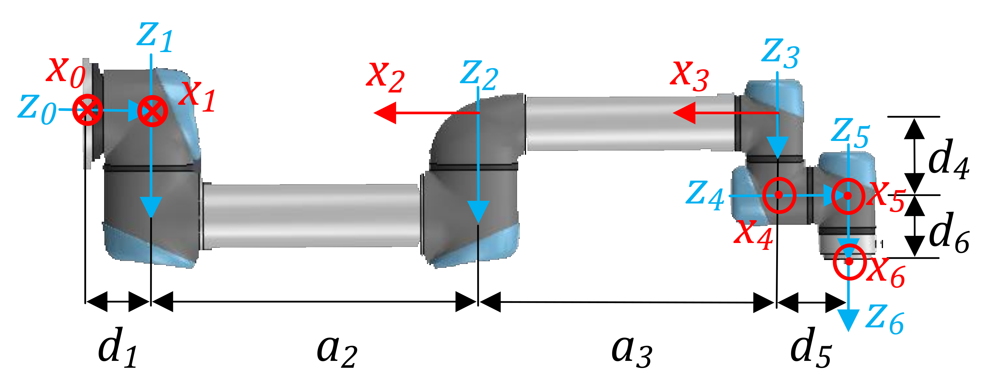
In this paper, we use a multi-degree-of-freedom vehicle-mounted tele-manipulator as the control object of the tele-aiming system, in which a camera is installed at the end of the tele-manipulator, and the camera image can be sent to the monitor through wireless image transmission equipment. According to the movement of the maneuvering target displayed in the monitoring video, the operator quickly controls the HCI device to generate the corresponding time-varying trajectory to control the tele-manipulator. For a rigid n-degree-of-freedom tele-manipulator, its dynamic equation can be expressed as:

$$N\left(q\right)\ddot{q}+V(q,\dot{q})\dot{q}+G\left(q\right)+S\left(\dot{q}\right)+d(q,\dot{q},\ddot{q},t)=\tau$$

(1)

where $q,\dot{q},\ddot{q}\in R^{n\times 1}$ denotes the joint angle, velocity, and acceleration, respectively; $N\left(q\right)\in R^{n\times n}$ denotes the inertia matrix; $V\left(q,\dot{q}\right)\in R^{n\times n}$ denotes the nonlinear Coriolis and centrifugal force; $G\left(q\right)\in R^{n\times 1}$ represents gravity; $S\left(\dot{q}\right)\in R^{n\times 1}$ is friction; $d\in R^{n\times 1}$ is external disturbance; $\tau \in R^{n\times 1}$ expresses the joint torque.

In practical applications, accurate robot model information is usually difficult to obtain, whereas only the nominal robot model can be acquired. The nominal model of the tele-manipulator is assumed as $N_0\left(q\right),V_0\left(q,\dot{q}\right),G_0\left(q\right)$. Setting $N=N_0+\Delta N,V=V_0+\Delta V,G=G_0+\Delta G$ and combining with the kinetic equation, we can get:

$$\left[N_0\left(q\right)+\Delta N\right]\ddot{q}+\left[V_0\left(q,\dot{q}\right)+\Delta V\right]\dot{q}+G_0\left(q\right)+\Delta G+S\left(\dot{q}\right)+d\left(t\right)=\tau$$

(2)

Accordingly,

$$N_0\left(q\right)\ddot{q}+V_0\left(q,\dot{q}\right)\dot{q}+G_0\left(q\right)=\tau +{\tau }_d(q,\dot{q},\ddot{q},t)$$

(3)

where ${\tau }_d(q,\dot{q},\ddot{q},t)\in R^{n\times 1}$ represents the unmodeled term, friction, and unknown disturbance of the tele-manipulator, as expressed below: ${\tau }_d\left(q,\dot{q},\ddot{q},t\right)=-\Delta N\ddot{q}-\Delta V\dot{q}-\Delta G-S\left(\dot{q}\right)-d\left(t\right)$.

If $x_1=q,x_2=\dot{q},\tau =u$ is defined, we can get the state-space equation by rewriting the above equation:

$$\left\{\begin{array}{cc}\hfill \dot{x_1}& =x_2\hfill \\ \hfill \dot{x_2}& =F\left(x_1,x_2\right)+B\left(x_1\right)u+D(x_1,x_2,t)\hfill \\ \hfill y& =x_1+v\hfill \end{array}\right.$$

(4)

where y is the measurement value of joint angle, and $v\in R^{n\times 1}$ is the measurement noise; $B\left(x_1\right)={N_0\left(x_1\right)}^{-1},F\left(x_1,x_2\right)=-{N_0\left(x_1\right)}^{-1}[V_0\left(x_1,x_2\right)x_2+G_0\left(x_1\right)],D(x_1,x_2,t)={N_0\left(x_1\right)}^{-1}{\tau }_d.$

In addition, we design a saturation function to prevent the joint torque u from exceeding the upper or lower limit, which is shown as follows:

$$u=\left\{\begin{array}{ccc}\hfill {\tau }_u,& \hfill & \hfill \tau >{\tau }_u\\ \hfill \tau ,& \hfill & \hfill -{\tau }_l\le \tau \le {\tau }_u\\ \hfill -{\tau }_l,& \hfill & \hfill \tau <-{\tau }_l\end{array}\right.$$

(5)

where ${\tau }_u$ and ${\tau }_l$ are the upper limit value and the lower limit value of the joint torque.

To efficiently tele-control the robot to aim at the maneuvering target, the operator should efficiently generate the time-varying non-uniform guidance trajectory through an HCI device (e.g., mouse or force feedback handle), and the guidance trajectory will be transformed into the desired joint trajectory corresponding to the joint space through the IK (inverse kinematics algorithm). Lastly, the proposed controller enables the respective joint of the tele-manipulator to track the corresponding joint trajectory, in which the desired joint trajectory includes the desired joint angle $q_d$, speed ${\dot{q}}_d$ and acceleration ${\ddot{q}}_d$.

The purpose of the controller designed in this study is to make the joint angle $x_1$ and speed $x_2$ track the non-uniform trajectories $q_d$ and ${\dot{q}}_d$ generated by the HCI device in real-time efficiently, stably, and accurately. The joint position tracking errors and velocity tracking errors are expressed as follows:

$$\left\{\begin{array}{c}\hfill e=x_1-q_d\\ \hfill \dot{e}=x_2-{\dot{q}}_d\end{array}\right.$$

(6)

Thus, the goal of this study is to design a controller that can make the error expressed by the above equation approach zero efficiently and stably in a limited time.

3. System Design

3.1. Tele-Aiming Robot System Overall Design

The tele-manipulator system, which is the control object of the tele-aiming system studied in this paper, is a highly coupled nonlinear system with multiple inputs and multiple outputs. Accordingly, when the time-varying non-uniform guidance trajectory is applied to the tele-manipulator, each joint of the tele-manipulator also should perform the time-varying non-uniform rapid steering movement. Due to the existence of inertia, each joint of the tele-manipulator will cause inertial impact force disturbance to other joints during rapid steering movement. Since the joints of the tele-manipulator are highly coupled, the whole tele-manipulator may not be able to achieve stable target tracking as impacted by coupling disturbance. To weaken the influence of inertial impact force disturbance and achieve fast time-varying non-uniform target tracking, this study proposes an active disturbance rejection terminal sliding mode guidance controller based on a multiple-model augmented-state extended Kalman observer. The proposed controller can efficiently eliminate the inertial impact force disturbance and achieve stable target tracking when the tele-manipulator is controlled by the tele-aiming control system. The overall structure of the tele-aiming control system is presented in Figure 1.

According to Figure 1, to eliminate the coupling inertial impact force disturbance, the multi-input multi-output nonlinear and strong coupling tele-manipulator system is first decoupled into a single-input single-output joint group, and the internal friction, parameter perturbation, modeling error, and other uncertain factors of the joint together with the inertial impact force disturbance are considered as a lumped disturbance. Subsequently, the lumped disturbance is estimated by MEKO. Lastly, the lumped disturbance is eliminated by the active disturbance rejection terminal sliding mode controller, and the respective joint can efficiently, accurately, and stably track the joint trajectory corresponding to the end guidance trajectory, to achieve the fast, stable, and high-precision end guidance control by the HCI device.

To achieve joint decoupling, we define $x={\left[x_1{x}_2\cdots x_n\right]}^T$,$F={\left[F_1{F}_2\cdots F_n\right]}^T$,$u={\left[u_1{u}_2\cdots u_n\right]}^T$,$D={\left[D_1{D}_2\cdots D_n\right]}^T$. For the multi-input multi-output nonlinear affine system expressed by the Equation (4), a “virtual control variable”: $U=B\left(x_1\right)u$ is introduced in this study, where $U={\left[U_1{U}_2\cdots U_n\right]}^T$, and then the (4) becomes:

$$\left\{\begin{array}{cc}\hfill \ddot{x}& =F\left(x\right)+U+D\left(x,t\right)\hfill \\ \hfill y& =x+v\hfill \end{array}\right.$$

(7)

The i-th joint in the robot system (4) turns out to be:

$$\left\{\begin{array}{cc}\hfill {\dot{x}}_{i1}& =x_{i2}\hfill \\ \hfill {\dot{x}}_{i2}& =F_i(x_{i1},x_{i2})+U_i+D_i\left(x_{i1},x_{i2},t\right)\hfill \\ \hfill y_i& =x_{i1}+v_i\hfill \end{array}\right.$$

(8)

where the input of the i-th joint is $U_i$, and its output is $y_i$, $v_i$ is the measurement noise on the corresponding joint channel. Thus, the input $U_i$ and output $y_i$ of each joint is a single-input single-output relationship. That is, the relationship between input $U_i$ and output $y_i$ of the i-th joint is completely decoupled. $D_i\left(x_{i1},x_{i2},t\right)$ represents the lumped disturbance of the i-th joint, including the inertial impact force disturbance attributed to rapid maneuvering traction.

The actual control torque $u={\left[u_1{u}_2\cdots u_n\right]}^T$ of the tele-manipulator is expressed by the virtual control variable $U={\left[U_1{U}_2\cdots U_n\right]}^T$. To weaken the chattering of the control torque, we carry out a low-pass filter (LPF) on the actual joint torque control sequence, as expressed below:

$$u=LPF\left(B^{-1}U\right)$$

(9)

3.2. MEKO-Based Active Disturbance Rejection Terminal Sliding Mode Controller

To enable the end of n-joint tele-manipulator to aim at the maneuvering target efficiently, the guidance trajectory generated by the HCI device is first converted into joint trajectories by using inverse kinematics. Then, the n-joint tele-manipulator system is decoupled and a single joint trajectory tracking controller is applied to every single joint. To achieve state estimation and disturbance estimation under measurement noises simultaneously, the single joint trajectory tracking controller is designed as an active disturbance rejection terminal sliding mode controller based on MEKO.

Its schematic diagram is presented in Figure 2. First, the tracking differentiator is adopted to pre-filter the reference joint trajectory and extract its speed information. Next, the MEKO is used to estimate the position, velocity, and disturbance of the respective joint simultaneously. Lastly, the nonsingular terminal sliding mode control algorithm is used to eliminate the disturbance term and drive the joint to track the corresponding trajectory with low chattering and minimum tracking errors. The reference acceleration processed by the recursive average filter (RAF) is used in the nonsingular terminal sliding mode control.

3.3. Tracking Differentiator

To aim at the maneuvering target, the operator generates the guidance trajectory with time-varying, non-uniform, and random abrupt motion characteristics by the HCI device. The guidance trajectory may also exist measurement noise disturbance. To ensure that the tele-manipulator system is capable of tracking the guidance trajectory with measurement noise and abrupt motion, in this study, a tracking differentiator (TD) was adopted to preprocess the reference joint trajectory. The TD is expressed as:

$$\left\{\begin{array}{cc}\hfill x_{i1d}\left(k+1\right)& =x_{i1d}\left(k\right)+h·x_{i2d}\left(k\right)\hfill \\ \hfill x_{i2d}\left(k+1\right)& =x_{i2d}\left(k\right)+h·fhan\left(x_{i1d}\left(k\right)-{\theta }_{id},x_{i2d}\left(k\right),r_{i0},h_{i0}\right)\hfill \end{array}\right.$$

(10)

where $x_{i1d}$ and $x_{i2d}$ denote the desired position and velocity of the i-th joint, respectively, h is the sampling period, and ${\theta }_{id}$ is the reference input signal, $r_{i0}$ represents the parameter of tracking speed, $h_{i0}$ is the step size different from h, $fhan\left(x_{i1d}\left(k\right)-{\theta }_{id},x_{i2d}\left(k\right),r_{i0},h_{i0}\right)$ is expressed as:

$$\left\{\begin{array}{cc}\hfill d_0& =r_{i0}{h_{i0}}^2,a_0=h_{i0}{x}_{i2d},y_0=x_{i1d}+a_0\hfill \\ \hfill a_1& =\sqrt{d_0\left(d_0+8\left|y_0\right|\right)}\hfill \\ \hfill a_2& =a_0+\frac{sign\left(y_0\right)\left(a_1-d_0\right)}{2}\hfill \\ \hfill s_1& =\frac{\left[sign\left(y_0+d_0\right)-sign\left(y_0-d_0\right)\right]}{2}\hfill \\ \hfill a_3& =\left(a_0+y_0-a_2\right)s_1+a_2\hfill \\ \hfill s_2& =\frac{\left[sign\left(a_3+d_0\right)-sign\left(a_3-d_0\right)\right]}{2}\hfill \\ \hfill fhan& =-r_{i0}\left[\frac{a_3}{d_0}-sign\left(a_3\right)\right]s_2-r_{i0}sign\left(a_3\right)\hfill \end{array}\right.$$

(11)

Through Equations (10) and (11), the tracking differentiator can efficiently pre-filter the input reference signal ${\theta }_{id}$ and extract the approximate differential signal simultaneously, even when ${\theta }_{id}$ is mixed with random offset noise generated by rapid maneuvering.

3.4. Multiple-Model Augmented-State Extended Kalman Observer

When the tele-manipulator is quickly guided by the HCI device, the joints will inertially impact other joints, which will cause instantaneous large residuals between the actual trajectory and the guidance trajectory. After converting to the joint space, such an instantaneous large residual will cause the guidance joint trajectory to vary suddenly, resulting in a sudden increase of the instantaneous tracking error. This inertial impact force disturbance can be considered as lumped disturbance together with internal friction, parameter perturbation, modeling error, and other uncertain factors. If this lumped disturbance can be estimated, it can be eliminated before it adversely affects the tele-aiming system. As we all know, the observer-based control methods can achieve a better control effect by estimating the lumped disturbance with a disturbance observer. To speed up the elimination of instantaneous tracking error, it is usually necessary to increase the observer gain, but this amplifies the measurement noise and may cause the flutter or instability.

In this paper, we propose a novel multiple-model augmented-state extended Kalman observer (MEKO) to achieve lumped disturbance estimation and noise filtering simultaneously. According to the second-order system expressed by (8), $F_i(x_{i1},x_{i2})$ denotes the partial known model. If $D_i\left(x_{i1},x_{i2},t\right)$ in (8) is considered as an extended state $x_{i3}$ and assuming that $D_i\left(x_{i1},x_{i2},t\right)$ is differentiable, and its derivative is bounded, (8) can be written as:

$$\left\{\begin{array}{cc}\hfill {\dot{x}}_{i1}& =x_{i2}\hfill \\ \hfill {\dot{x}}_{i2}& =F_i(x_{i1},x_{i2})+U_i+x_{i3}\hfill \\ \hfill {\dot{x}}_{i3}& ={\dot{D}}_i\left(x_{i1},x_{i2},t\right)\hfill \\ \hfill y_i& =x_{i1}+v_i\hfill \end{array}\right.$$

(12)

If $x_{i1}=y_i,x_{i2}=\dot{y_i},x_{i3}=D_i\left(x_{i1},x_{i2},t\right)$ is defined and $D_i\left(x_{i1},x_{i2},t\right)$ is considered as process noise, then (12) is further rewritten as:

$$\left\{\begin{array}{cc}\hfill {\dot{X}}_i& =f\left(x_i,U_i\right)+w_i\hfill \\ \hfill y_i& =x_{i1}+v_i\hfill \end{array}\right.$$

(13)

where $f\left(x_i,U_i\right)=\left[\begin{array}{c}{x}_{i2}\\ F_i(x_{i1},x_{i2})+U_i+x_{i3}\\ 0\end{array}\right];w_i=\left[\begin{array}{c}0\\ 0\\ D_i\left(x_{i1},x_{i2},t\right)\end{array}\right];C=\left[\begin{array}{ccc}1& 0& 0\end{array}\right]$.

The above equation can be expressed approximately in discrete form, then we get:

$$\left\{\begin{array}{cc}\hfill Z_i\left(k\right)& =f[Z_i(k-1),U_i(k-1)]+W_i(k-1)\hfill \\ \hfill Y_i& \left(k\right)=C{Z}_i\left(k\right)+V_i\left(k\right)\hfill \end{array}\right.$$

(14)

where $Z_i{=\left[\begin{array}{ccc}{z}_{i1}& z_{i2}& z_{i3}\end{array}\right]}^T$ is the state vector of the discrete system, k represents the number of samples, $W_i$ and $V_i$ are the uncorrelated process noise and measurement noise.

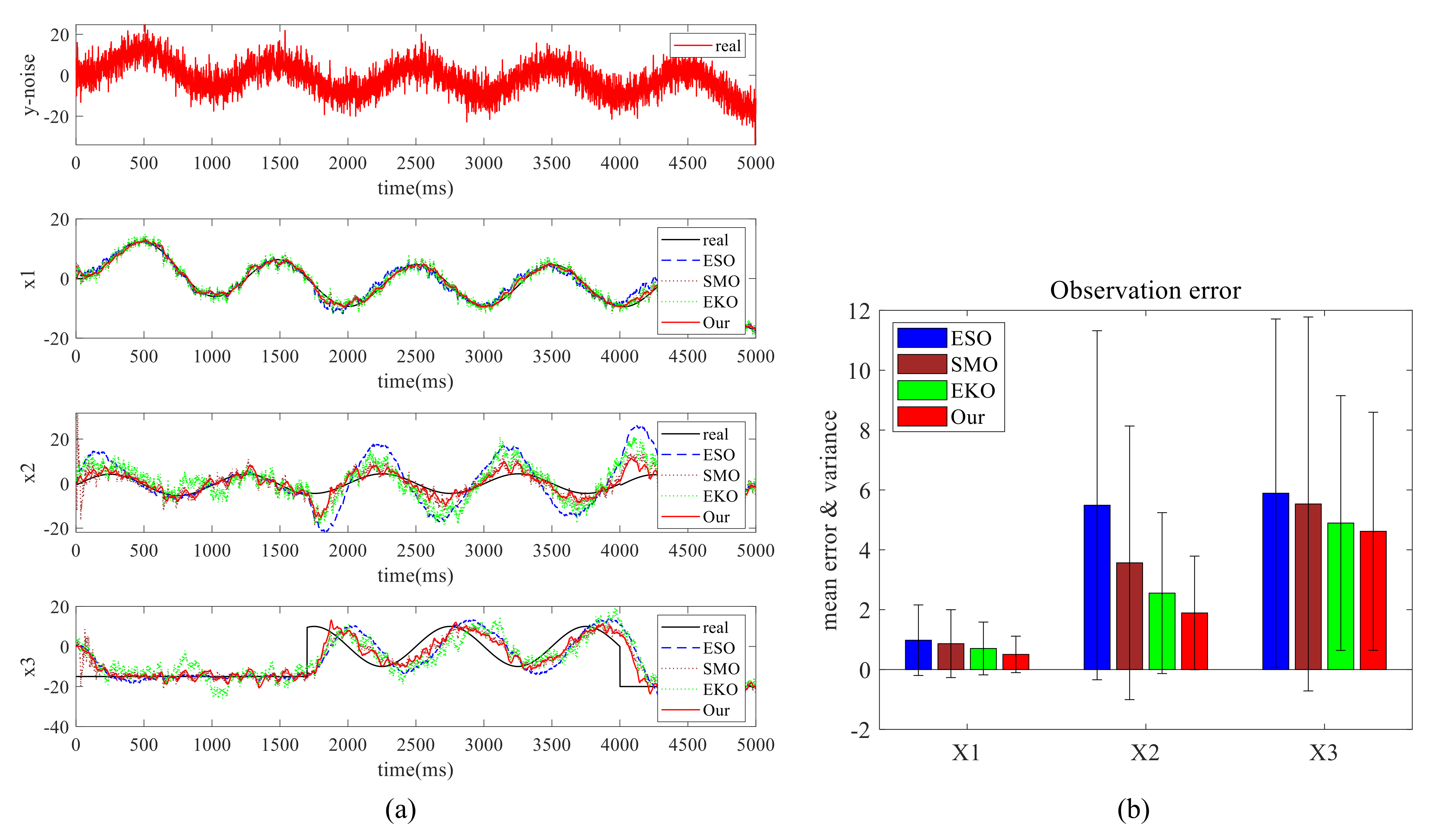
To estimate the disturbance and filter the measurement noise simultaneously, we propose a novel MEKO based on an extended Kalman observer (EKO). If ${\widehat{Z}}_i{=\left[\begin{array}{ccc}{\widehat{z}}_{i1}& {\widehat{z}}_{i2}& {\widehat{z}}_{i3}\end{array}\right]}^T$ is defined, EKO can realize state estimation, that is ${\widehat{Z}}_i\to Z_i$. Its principle is to treat the system modeling error and external disturbance as process noise, then expand it into a new system state and finally estimate it. Its basic principle is the same as that of Luenberger observer and ESO. However, compared with Luenberger observer and ESO, EKO can achieve the optimal estimation under linear minimum variance. In practical application, the external disturbance of the robot system may be a constant disturbance, time-varying disturbance, or instantaneous impact disturbance, which makes it difficult for us to determine the statistical characteristics of disturbance noise.

In this paper, to make the observer adapt to the disturbance noise with different statistical characteristics, the proposed MEKO optimize the weighted value of each observer online by using the estimation of innovation variance, so as to make the MEKO output the optimal disturbance estimation value according to the statistical characteristics of disturbance noise in the preset range. As shown in Figure 3, the output of the MEKO is the weighted average of a group of EKO outputs.

The convergence proof of EKO (basic observer of MEKO) is given in references [38,39], i.e., the EKO can achieve ${\widehat{z}}_{i1}\to x_{i1},{\widehat{z}}_{i2}\to x_{i2},{\widehat{z}}_{i3}\to x_{i3}=D_i\left(x_{i1},x_{i2},t\right)$.

The pseudo-code of MEKO is shown in Algorithm 1 as follows:

Algorithm 1: Multiple-model augmented-state Extended Kalman Observer (MEKO)

1: Initialization: sliding window width of innovation sequence: $N_i$, model number: $M_i$, process noise variance matrices: $Q_{i,m}\in {\mathbb{R}}^{3\times 3\times M_i}$, measurement noise variance matrices: $R_{i,m}\in {\mathbb{R}}^{1\times 1}$, prior error covariance matrices: $P_{i,m}\left(0\right)\in {\mathbb{R}}^{3\times 3}$ 2: Get the current sampling time: k = 1,2,… 3: for$m=1:M_i$do 4:    Compute: Jacobian matrix ${\Phi }_{i,m}\left(k\right)$ 5:    ${\left.{\Phi }_{i,m}\left(k\right)=\frac{\partial f[{\widehat{Z}}_{i,m}(k-1),U_{i}m(k-1)]}{\partial {\widehat{Z}}_{i,m}^T(k-1)}\right|}_{{\widehat{Z}}_{i,m}\left(k-1\right)=Z_{i,m}(k-1)}$ 6:    Predict: prior system state ${\widehat{Z}}_{i,m}^{-}$ and the prior error covariance $P_{i,m}^{-}$ 7:    ${\widehat{Z}}_{i,m}^{-}\left(k\right)=f[{\widehat{Z}}_{i,m}(k-1),U_{i,m}(k-1)]$ 8:    $P_{i,m}^{-}\left(k\right)={\Phi }_{i,m}\left(k\right)P_{i,m}\left(k-1\right){\Phi }_{i,m}^T\left(k\right)+Q_{i,m}\left(k\right)$ 9:    Update: Kalman gain $K_{i,m}$ 10:    $K_{i,m}\left(k\right)=\frac{P_{i,m}^{-}\left(k\right)C^T}{{CP}_{i,m}^{-}\left(k\right)C^T+R_{i,m}\left(k\right)}$ 11:    Correct: posterior system state ${\widehat{Z}}_{i,m}$ and the posterior error covariance $P_{i,m}$ 12:    ${\widehat{Z}}_{i,m}\left(k\right)={\widehat{Z}}_{i,m}^{-}\left(k\right)+K_{i,m}\left(k\right)[Y_i\left(k\right)-C{\widehat{Z}}_{i,m}^{-}\left(k\right)]$ 13:    $P_{i,m}\left(k\right)=[I-K_{i,m}\left(k\right)C]P_{i,m}^{-}\left(k\right)$ 14:    Compute: Innovation ${IV}_{i,m}$ and innovation covariance ${CIV}_{i,m}$ 15:    if $k\le N_i$ then 16:      ${IV}_{i,m}\left(k\right)=Y_{i,m}\left(k\right)-C{\widehat{Z}}_{i,m}^{-}\left(k\right)$ 17:    else 18:      for $j=2:N_i$ do 19:         ${IV}_{i,m}(j-1)={IV}_{i,m}\left(j\right)$ 20:      end for 21:      ${IV}_{i,m}\left(N_i\right)=Y_{i,m}\left(k\right)-C{\widehat{Z}}_{i,m}^{-}\left(k\right)$ 22:    end if 23:    ${CIV}_{i,m}\left(k\right)=\frac{1}{N_i}{\sum }_{j=k-N_i+1}^k{IV}_{i,m}\left(j\right){{IV}_{i,m}\left(j\right)}^T$ 24: end for 25: for$m=1:M_i$do 26:    ${\omega }_{i,m}\left(k\right)=\frac{1/{CIV}_{i,m}\left(k\right)}{{\sum }_{m=1}^{M_i}1/{CIV}_{i,m}\left(k\right)}$ 27: end for 28: ${\widehat{Z}}_i\left(k\right)={\sum }_{m=1}^{M_i}{\omega }_{i,m}\left(k\right){\widehat{Z}}_{i,m}\left(k\right)$

It can be seen from the above pseudo-code that the weight of each EKO in MEKO is adjusted online according to the optimal estimation of innovation covariance. That is, if the innovation variance of an EKO is smaller, the estimated value of the EKO is accurate, and the weight of the EKO in the bank of EKOs is larger. By automatically adjusting the weights, a bank of EKOs with preset process statistical characteristics can output the optimal observation value in real-time according to the innovation and its covariance.

Strictly speaking, the proposed multiple-model observer-based control method belongs to the scope of data-driven control. The control effect of common data-driven control highly depends on the training data. It learns the controlled object without constraints, and its final learning is uncertain, and its stability cannot be well guaranteed. However, the proposed method does not directly use the input and output data to learn the controlled object or adjust the parameters of the controller, as in reference [40], but uses the measured output data to adjust the weight of each observer in the multiple-model observer, and finally outputs the lumped disturbance value according to the weighted sum of all observers. Different from the common data-driven methods, our method still belongs to model-based control, but the unmodeled dynamics and external disturbance can be observed in real-time through the data-driven method and eliminated in the subsequent control stage.

3.5. Nonsingular Terminal Sliding Mode Controller

Sliding mode control exhibits the advantages of simple, fast response, and strong robustness to external disturbances, unmodeled dynamics, and parameter perturbation. Compared with linear sliding mode control, terminal sliding mode enhances the convergence characteristics exhibited by the system by adding nonlinear terms into the sliding mode surface. It is characterized by the advantages of fast dynamic response, finite-time convergence, and high steady-state tracking accuracy. To further improve the robustness of the control system, a nonsingular terminal sliding mode control law is added into the nonlinear feedback control in the active disturbance rejection control framework.

First, the trajectory tracking error of i-th joint is defined as $e_{i1}=x_{i1}-x_{i1d}$, and the nonsingular sliding mode surface function is defined as:

$$s_i=e_{i1}+\frac{1}{{\beta }_i}{{\dot{e}}_{i1}}^{\frac{p_i}{q_i}}$$

(15)

where ${\beta }_i>0,p_i,q_i(p_i>q_i)$ are positive odd numbers.

The nonsingular terminal sliding mode controller is designed as:

$${\tau }_{ntsmc\_i}={\ddot{x}}_{i1d}-{\beta }_i\frac{q_i}{p_i}{{\dot{e}}_{i1}}^{2-\frac{p_i}{q_i}}-{\eta }_{i}sign\left(s_i\right)$$

(16)

In practical applications, to further suppress chattering, the saturation function $sats\left(s_i\right)$ is generally adopted to replace the sign function $sign\left(s_i\right)$ in the above equation, and its expression is:

$$sats\left(s_i\right)=\left\{\begin{array}{cc}\hfill sign\left(s_i\right),& \left|s_i\right|>{\delta }_i\hfill \\ \hfill \frac{s_i}{{\delta }_i},& \left|s_i\right|\le {\delta }_i\hfill \end{array}\right.$$

(17)

Compared with the conventional sign function, the saturation function can make the system adopt different strategies by complying with the value of sliding mode, i.e., outside the boundary layer ${\delta }_i$, the switching control is adopted to make the system state efficiently tend to slide mode. At the boundary layer ${\delta }_i$, the feedback control is adopted to reduce the chattering attributed to the rapid switching of sliding modes and ensure the function $s_i$ to be constantly at the boundary layer.

Generally, the acceleration signal is obtained by using the second-order difference method. Since the rapid random non-uniform tele-aiming control generates a guidance trajectory with an abrupt signal, the conventional second-order difference method will introduce amplified noise when processing this signal. Accordingly, to reduce the effect of the noise signal in the desired joint acceleration on the joint control, the recursive average filter (RAF) is exploited to process the desired joint acceleration ${\ddot{x}}_{i1d}$, as expressed below:

$${\ddot{q}}_{id}\left(k\right)=\left\{\begin{array}{cc}\hfill {\ddot{x}}_{i1d}\left(k\right),& k\le N\hfill \\ \hfill \frac{{\sum }_{j=k-N}^k{\ddot{x}}_{i1d}\left(j\right)}{N},& k>N\hfill \end{array}\right.$$

(18)

In this study, the MEKO is adopted to achieve the real-time online estimation of system state and lumped disturbance under the measurement noise, i.e., ${\widehat{z}}_{i1}\to x_{i1},{\widehat{z}}_{i2}\to x_{i2},{\widehat{z}}_{i3}\to x_{i3}$. Thus, the trajectory tracking error of the i-th joint is actually ${\widehat{e}}_{i1}={\widehat{z}}_{i1}-x_{i1d},{\widehat{e}}_{i2}={\widehat{\dot{e}}}_{i1}={\widehat{z}}_{i2}-x_{i2d}$, so the nonsingular terminal sliding mode controller of the i-th joint under the MEKO is modified as:

$$U_i={\ddot{q}}_{id}-{\beta }_i\frac{q_i}{p_i}{{\widehat{\dot{e}}}_{i1}}^{2-\frac{p_i}{q_i}}-{\eta }_{i}sats\left({\widehat{s}}_i\right)-F_i\left(x_{i1},x_{i2}\right)-{\widehat{z}}_{i3}$$

(19)

where ${\widehat{s}}_i={\widehat{e}}_{i1}+\frac{1}{{\beta }_i}{{\widehat{\dot{e}}}_{i1}}^{\frac{p_i}{q_i}}$ is the estimated value of nonsingular sliding mode surface function.

To reduce the chatter of the controller’s output signal, we perform a low-pass filter (LPF) on the controller’s output signal before sending it to robot, as expressed below:

$${\tau }_i=LPF\left(B^{-1}\left(U_i\right)\right)$$

(20)

3.6. Stability Proof of Closed-Loop Control System

In this paper, ${\widehat{\ddot{x}}}_{i1}={\ddot{x}}_{i1}+{\Delta }_i$ is defined, and ${\Delta }_i={\widehat{\ddot{x}}}_{i1}-{\ddot{x}}_{i1}={\widehat{z}}_{i3}-D_i\left(x_{i1},x_{i2},t\right)$ is set as the estimation error of the expanded state. The Lyapunov function of the i-th joint is taken as $V_{is}={0.5{\widehat{s}}_i}^2$, then the Lyapunov derivative is as follows.

$$\begin{array}{cc}\hfill {\dot{V}}_{is}& ={{\widehat{s}}_i\widehat{\dot{s}}}_i\hfill \\ \hfill & ={\widehat{s}}_i\left({\widehat{\dot{e}}}_{i1}+\frac{1}{{\beta }_i}\frac{p_i}{q_i}{{\widehat{\dot{e}}}_{i1}}^{\frac{p_i}{q_i}-1}{\widehat{\ddot{e}}}_{i1}\right)\hfill \\ \hfill & ={\widehat{s}}_i\left({\widehat{\dot{e}}}_{i1}+\frac{1}{{\beta }_i}\frac{p_i}{q_i}{{\widehat{\dot{e}}}_{i1}}^{\frac{p_i}{q_i}-1}\left({\widehat{\ddot{x}}}_{i1}-{\ddot{q}}_{id}\right)\right)\hfill \\ \hfill & ={\widehat{s}}_i\left({\widehat{\dot{e}}}_{i1}+\frac{1}{{\beta }_i}\frac{p_i}{q_i}{{\widehat{\dot{e}}}_{i1}}^{\frac{p_i}{q_i}-1}\left({\ddot{x}}_{i1}+{\Delta }_i-{\ddot{q}}_{id}\right)\right)\hfill \\ \hfill & ={\widehat{s}}_i\left({\widehat{\dot{e}}}_{i1}+\frac{1}{{\beta }_i}\frac{p_i}{q_i}{{\dot{\widehat{e}}}_{i1}}^{\frac{p_i}{q_i}-1}\left(F_i\left(x_{i1},x_{i2}\right)+U_i+D_i\left(x_{i1},x_{i2},t\right)+{\Delta }_i-{\ddot{q}}_{id}\right)\right)\hfill \\ \hfill & ={\widehat{s}}_i\left({\widehat{\dot{e}}}_{i1}+\frac{1}{{\beta }_i}\frac{p_i}{q_i}{{\widehat{\dot{e}}}_{i1}}^{\frac{p_i}{q_i}-1}\left(-{\beta }_i\frac{q_i}{p_i}{{\widehat{\dot{e}}}_{i1}}^{2-\frac{p_i}{q_i}}-{\eta }_{i}sats\left(\widehat{s}\right)-{\widehat{z}}_{i3}+D_i\left(x_{i1},x_{i2},t\right)+{\Delta }_i\right)\right)\hfill \\ \hfill & ={\widehat{s}}_i\left(\frac{1}{{\beta }_i}\frac{p_i}{q_i}{{\widehat{\dot{e}}}_{i1}}^{\frac{p_i}{q_i}-1}\left(-{\eta }_{i}sats\left(\widehat{s}\right)-{\widehat{z}}_{i3}+D_i\left(x_{i1},x_{i2},t\right)+{\Delta }_i\right)\right)\hfill \\ \hfill & ={\widehat{s}}_i\left(\frac{1}{{\beta }_i}\frac{p_i}{q_i}{{\widehat{\dot{e}}}_{i1}}^{\frac{p_i}{q_i}-1}\left(-{\eta }_{i}sats\left(\widehat{s}\right)\right)\right)\hfill \\ \hfill & =-{{\eta }_i}^{\prime }\left|{\widehat{s}}_i\right|\hfill \end{array}$$

(21)

where ${{\eta }_i}^{\prime }=\frac{1}{{\beta }_i}\frac{p_i}{q_i}{{\widehat{\dot{e}}}_{i1}}^{\frac{p_i}{q_i}-1}{\eta }_i$.

When ${\dot{\widehat{e}}}_{i1}\ne 0$, $\frac{1}{{\beta }_i}\frac{p_i}{q_i}{{\widehat{\dot{e}}}_{i1}}^{\frac{p_i}{q_i}-1}{\eta }_i>0$, the above equation ${\dot{V}}_{is}=-{{\eta }_i}^{\prime }\left|{\widehat{s}}_i\right|\le 0$, which indicates that the system is stable. As indicated from reference [21], the sliding mode function $s_i$ can approach zero in a finite time. It is therefore suggested that the closed-loop control system of the i-th joint is stable, and the sliding mode surface is reachable.

When the closed-loop control system of each joint can ensure stability and the sliding mode surface can be reached, the closed-loop control system of the robot is also stable, and the sliding mode surface can be reached. In other words, when t approaches infinity, s, e, $\dot{e}$ approaches zero, i.e., $t\to \infty ,s\to 0,e\to 0,\dot{e}\to 0$. To be specific, the proposed MEKO-based nonsingular terminal sliding mode controller can make (6) stable to zero.

4. Simulation Results and Discussions

4.1. Disturbance Observation Experiment

To verify the effectiveness of our proposed MEKO, we set up a comparative experiment of disturbance observation. The observed object is shown as follows:

$$\left\{\begin{array}{cc}\hfill \dot{x_1}& =x_2\hfill \\ \hfill \dot{x_2}& =F\left(x_1,x_2\right)+bu+D(x_1,x_2,t)\hfill \\ \hfill y& =x_1+v\hfill \end{array}\right.$$

(22)

where, $F\left(x_1,x_2\right)=-25x_2$, $b=120$ are the known parts, $D(x_1,x_2,t)$ is the unknown lumped part, the input torque signal $u=sin\left(0.2\ast \pi \ast t\right)$ was in the form of the sine wave. The initial position and initial velocity of the observed object were taken as zero. The simulation step was set to 0.01, and the total number of simulation steps was 5000 time steps.

To verify the multi disturbance observation ability of the observer, the lumped disturbance used the following piecewise function:

$$D\left(x_1,x_2,t\right)=\left\{\begin{array}{cc}\hfill -15,& t<1700\hfill \\ \hfill -10\ast sin\left(0.2\ast \pi \ast t\right),& 1000\le t\le 4000\hfill \\ \hfill -20,& t>4000\hfill \end{array}\right.$$

(23)

The contrast observer used extended state observer ESO [30,41], high-order sliding mode observer SMO [21], and extended state Kalman observer EKO [42], respectively.

Table 1. Observer parameter setting.

Observer	Parameter Setting
ESO	${\beta }_{i1}=3\ast \omega ,{\beta }_{i2}=3\ast {\omega }^2,{\beta }_{i3}=2\ast {\omega }^3,\omega =2,{\alpha }_{i1}=0.5,{\alpha }_{i2}=0.25,{\delta }_i=10h$
SMO	${\gamma }_{i1}=30,{\gamma }_{i2}=80,{\gamma }_{i3}=100$
EKO	$P_i\left(0\right)=10000,R_i=200,Q_i=\left[\begin{array}{ccc}1& 0& 0\\ 0& 2& 0\\ 0& 0& 4\end{array}\right]$
Our MEKO	$N_i=10,M_i=60,P_{im}\left(0\right)=10,000,R_{im}=1000,Q_{im}=\left[\begin{array}{ccc}0.5\ast \gamma & 0& 0\\ 0& 1\ast {\gamma }^2& 0\\ 0& 0& 0.5\ast {\gamma }^3\end{array}\right],\gamma =1:M_i$

shows the parameters of all observers used in this experiment. These parameters are the optimal parameters obtained after many experiments.

To simulate the real system, we added measurement noise with a mean value of 0 and a variance of 20 to the output signal, as shown in Figure 4a. The experimental results in Figure 4a, respectively, show the results of the four observers in observing the first-order position signal, the second-order velocity signal, and the third-order lumped disturbance signal. The black solid line represents the actual signal, the blue dotted line represents the observation results of ESO, the brown dotted line represents the observation results of SMO, the green dotted line represents the observation results of EKO, and the red solid line represents the observation results of MEKO proposed in this study. The experimental results in Figure 4b show the observed mean error and variance of the four observers at the first-order position, the second-order velocity, and the third-order lumped disturbance.

As can be seen from Figure 4a, when observing the first-order position signal, the fluctuation of ESO and EKO is slightly larger in the case of measurement noise, while the filtering effect and tracking effect of SMO and our proposed observer are better. When observing the second-order velocity, the fluctuation of ESO and EKO is slightly larger, and the observation result of MEKO is relatively consistent with the actual velocity. When observing the lumped disturbance signal, the four observers have a certain degree of phase delay in the face of multiple disturbances, but generally speaking, the MEKO represented by the red curve is relatively consistent with the actual disturbance signal. It can also be seen from Figure 4b that ESO has the maximum observation mean error and variance, followed by SMO and EKO, while our proposed MEKO has the minimum error and variance in the observation of first-order position, second-order velocity and third-order lumped disturbance signal. This comparative experiment shows that our proposed MEKO has good estimation performance for multiple types of disturbance (two constant value disturbance and one sinusoidal disturbance) under measurement noise interference.

4.2. Trajectory Tracking Experimental Setup

To verify the effectiveness of the proposed control method, several simulation experiments were performed on the MATLAB and the CoppeliaSim simulation platform. The UR5 manipulator in the CoppeliaSim simulation platform was employed as the tele-aiming control experimental object. The D-H parameters and dynamics parameters of the UR5 are listed in

Table 2. D-H parameters and dynamic parameters of the UR5 robot.

Kinematics	Theta [rad]	d [m]	a [m]	Alpha [rad]	Dynamics	Mass [kg]	Center of Mass [m]
Joint1	${\theta }_1$	0.089159	0	$\pi$/2	Link1	3.7	[0, −0.02561, 0.00193]
Joint2	${\theta }_2$	0	−0.425	0	Link2	8.393	[0.2125, 0, 0.11336]
Joint3	${\theta }_3$	0	−0.39225	0	Link3	2.33	[0.11993, 0, 0.0265]
Joint4	${\theta }_4$	0.10915	0	$\pi /2$	Link4	1.219	[0, −0.0018, 0.01634]
Joint5	${\theta }_5$	0.09465	0	$-\pi /2$	Link5	1.219	[0, 0.0018, 0.01634]
Joint6	${\theta }_6$	0.0823	0	0	Link6	0.1879	[0, 0, −0.001159]

, and the coordinate system is presented in Figure 5. The simulation step size was set to 10 ms. The maximal joint torque of all joints is limited to 150 N (i.e., ${\tau }_u=150,{\tau }_l=150$), and its initial joint positions are [${90}^{\circ },-{160}^{\circ },{150}^{\circ },0^{\circ },{90}^{\circ },0^{\circ }$].

4.3. Uniform Trajectory Tracking Experiment

To verify the effectiveness of the MEKO-based active disturbance rejection nonsingular terminal sliding mode controller (MEKOTSMC) proposed in this study, the MEKOTSMC and other comparison controllers were applied to uniform trajectory tracking experiments.

In this experiment, the tuning parameters of the proposed MEKOTSMC were set as follows. In TD part: $r_{i0}=1600,h_{i0}=2h$; In NTSMC part: ${\beta }_i=46,{\eta }_i=300,p_i=9,q_i=7,{\delta }_i=0.2$; In MEKO part: the sliding window width of innovation sequence $N_i=10$, the model number $M_i=60$, the measurement noise variance matrices $R_{i,m}=1000$, the prior error covariance matrices $P_{i,m}\left(0\right)=10,000$, the process noise variance matrices $Q_{i,m}=\left[\begin{array}{ccc}1\ast \gamma & 0& 0\\ 0& 0.5\ast {\gamma }^2& 0\\ 0& 0& 0.05\ast {\gamma }^3\end{array}\right]$, where $\gamma =1:M_i$.

As a contrast, for the identical trajectory tracking experiment, this study employed the computed torque controller (CTC) [43], the terminal sliding mode controller based on the computed torque controller (CTC-NTSMC) [44], the computed torque controller based on radial basis function (RBF) neural network compensation (CTC-RBF)[45], the active disturbance rejection sliding mode controller (ADRSMC) [46], as well as the proposed controller (MEKOTSMC).

Table 3. Compared controller parameter setting.

Controller	Parameter Setting
CTC	$\tau =M_0\left({\ddot{q}}_d+K_{p}e+K_d\dot{e}+K_i\int edt\right)+C_0\left(q,\dot{q}\right)\dot{q}+G_0\left(q\right),K_p=100,K_d=2\sqrt{100},K_i=1$
CTC-RBF	$\tau =M_0\left({\ddot{q}}_d+K_{p}e+K_d\dot{e}+K_i\int edt\right)+C_0\left(q,\dot{q}\right)\dot{q}+G_0\left(q\right)+\widehat{f}\left(•\right)$
CTC-NTSMC	$\tau =M_0({\ddot{q}}_d-\beta \frac{q}{p}{e}^{2-\frac{p}{q}}-(D+\eta )sats\left(s\right))+C_0\left(q,\dot{q}\right)\dot{q}+G_0\left(q\right),\beta =20,\eta =0.1,D=800,p=9,q=7$
ADRSMC	$r_{i0}=1600,h_{i0}=2h,{\beta }_{i1}=60,{\beta }_{i2}=300,{\beta }_{i3}=600,{\alpha }_{i1}=0.5,{\alpha }_{i2}=0.25,{\delta }_i=10h,K_i=20,c_i=30$

shows the parameters of all controllers used in this experiment. These parameters are the optimal parameters obtained after many experiments.

In the CTC-RBF, the uncertainty $\widehat{f}\left(•\right)$ of the system was expressed by the output value of RBF neural network. There were five neurons at the hidden layer of RBF neural network, the radial basis function parameter was set to $c_i=\left[\begin{array}{ccccc}-2& -1& 0& 1& 2\end{array}\right]$, and other parameters complied with the CTC. For fairness, the reference joint acceleration ${\ddot{q}}_d$ in the comparison controllers had been processed with recursive average filter as well.

In this section, to verify the performance of the controllers, two groups of experiments were set:

• MEKOTSMC and comparison controllers were adopted to control the robot, respectively, to achieve uniform trajectory tracking without joint measurement noises. The experimentally obtained results are presented in Figure 6a,c,e;
• MEKOTSMC and comparison controllers were exploited to control the robot, respectively, to achieve uniform trajectory tracking with joint measurement noises (the joint measurement noise of [−0.05 rad ~0.05 rad] is randomly added). The experimentally obtained results are illustrated in Figure 6c,d,f.

The comparison results of the end motion trajectory are presented in Figure 6, in which Figure 6a shows the results without the addition of joint measurement noises, and Figure 6b shows the results under the addition of joint measurement noises. Figure 6c,d show the comparison of square root errors generated by five controllers in two cases, i.e., with or without joint measurement noises. Figure 6e,f show the comparison results of the mean error and variance diagram generated by the five controllers in two cases, i.e., with or without joint measurement noises. The comparison results reflect the average level of tracking error and the similarity between the tracking trajectory and the desired trajectory throughout the tracking.

As indicated in Figure 6a, for the uniform trajectory without joint measurement noises, the five controllers were all able to achieve stable tracking. From the square root error diagram in Figure 6c, it can be seen that CTC-NTSMC was able to efficiently reduce the tracking error at the initial stage of trajectory tracking of the robot. The tracking error of the proposed controller first increases slightly and then decreases rapidly at the initial stage of tracking, which also leads to a larger mean error than CTC-NTSMC. Compared with other controllers, the proposed controller performed slightly better in the middle and later stages of the tracking process. As presented in Figure 6e, CTC and CTC-RBF performed poorly, while CTC-NTSMC, ADRSMC, and the proposed controller in this study performed well. Among them, CTC-NTSMC produced the smallest mean error, i.e., for the uniform trajectory without joint measurement noises, CTC-NTSMC was able to enable the robot to achieve trajectory tracking with less error.

According to Figure 6b,d, for the uniform trajectory with joint measurement noises, CTC, CTC-RBF, and CTC-NTSMC all failed to track, and only ADRSMC and the proposed controller were able to achieve stable tracking. From the square root error diagram in Figure 6d, it can be seen that at the initial stage of trajectory tracking of the robot, the five controllers can efficiently reduce the tracking error, but CTC, CTC-RBF, and CTC-NTSMC have error divergence immediately. This shows that these three controllers have poor robustness in the presence of measurement noises, while ADRSMC and the proposed controller have good anti-noise ability in the face of joint measurement noises. As indicated in Figure 6f, the mean error and variance diagram of ADRSMC and the proposed controller are very close.

To show the performance of the five controllers in more detail, we show the mean error and variance of the respective joint generated when the five controllers were adopted to control the robot to track a uniform trajectory in Figure 7. Among them, Figure 7a,b show the mean error and variance of the joint without joint measurement noises and with joint measurement noises, respectively.

According to the error bar graph presented in Figure 7a, compared with CTC and CTC-RBF, the mean error and variance of each joint generated by CTC-NTSMC, ADRSMC, and the proposed controller are smaller. The error bar graph shown in Figure 7b reveals that ADRSMC and the proposed controller can achieve the minimal mean error and variance of the respective joint, while CTC, CTC-RBF, and CTC-NTSMC show noticeable obvious error divergence when controlling the 1st∼6th joint of the robot, which also accounts for the failure of tracking uniform trajectory.

In brief, Figure 6 and Figure 7 indicate that only ADRSMC and the proposed controller were able to enable the robot to achieve stable trajectory tracking for the uniform trajectory without joint measurement noises and with joint measurement noises, and there is an insignificant difference between the two.

4.4. Non-Uniform Maneuvering Target Trajectory Tracking Experiment

To more practically simulate the non-uniform maneuvering target and the performance of the tele-aiming control system, we generate a non-uniform maneuvering target trajectory by adding [−0.01 m~0.01 m] random offset noise to the circular trajectory radius. Subsequently, the controllers were adopted to control the robot to track this non-uniform trajectory. Furthermore, to verify the performance of the controllers under joint measurement noises, the following two groups of experiments were set:

• the proposed controller and the comparison controllers were adopted to control the robot to achieve non-uniform trajectory tracking without joint measurement noises. The experimentally obtained results are illustrated in Figure 8a,c,e;
• the proposed controller and the comparison controllers were adopted to control the robot to achieve non-uniform trajectory tracking with joint measurement noises (the joint measurement noise of [−0.05 rad~0.05 rad] is randomly added to simulate the sensor measurement noise in the actual robot system). The experimentally obtained results are presented in Figure 8b,d,f.

Figure 8a,b illustrate the end motion trajectory comparison diagram when the end of robot was controlled to track the non-uniform trajectory (two cases, i.e., joint measurement noises not added, and joint measurement noises added) by using the proposed controller and the four comparison controllers (i.e., CTC, CTC-RBF, CTC-NTSMC, and ADRSMC), respectively. Figure 8c,d compare the square root errors generated by the five controllers in two cases, i.e., with and without joint measurement noises. Figure 8e,f present the comparison diagrams of mean error and variance diagram generated by the five controllers in two cases, i.e., with or without joint measurement noises. The comparison diagram presents the average level of tracking error and the similarity between the tracking trajectory and the desired trajectory throughout the tracking.

According to Figure 8a, for the non-uniform trajectory without joint measurement noises, the five controllers were able to achieve stable tracking. As indicated in the square root error diagram in Figure 8c, the proposed controller first increases the tracking error slightly, then reduces the error rapidly, and then maintains it at a low level. Compared with other comparison controllers, the proposed controller performed slightly better at the middle and later tracking stages. According to Figure 8e, the mean error and variance of CTC and CTC-RBF are relatively large, while the mean error and variance of CTC-NTSMC, ADRSMC, and the proposed controller are relatively small. The proposed controller was the controller with the smallest mean error throughout the tracking, i.e., for the uniform trajectory without joint measurement noises, the proposed controller was able to make the robot achieve trajectory tracking with less error.

As presented in Figure 8b,d, for the uniform trajectory with joint measurement noises, CTC, CTC-RBF, and CTC-NTSMC all failed to track. Only ADRSMC and the proposed controller were capable of achieving stable tracking. From the square root error diagram in Figure 8d, at the initial stage of trajectory tracking, it can be seen that the five controllers were able to efficiently reduce the tracking error, whereas CTC, CTC-RBF, and CTC-NTSMC exhibit error divergence immediately. Thus, CTC, CTC-RBF, and CTC-NTSMC show poor robustness in the presence of measurement noises, while ADRSMC and the proposed controller exhibit a high anti-noise ability when facing joint measurement noises. According to Figure 8f, the mean error and variance diagram of the proposed controller is slightly smaller than those of ADRSMC and other comparison controllers, which reveals that the proposed controller can achieve stable tracking with small error even if the measurement noises are added when facing non-uniform trajectory.

To more intuitively illustrate the performance of the five controllers, the mean error and variance of each joint are presented when the five controllers were adopted to control the robot to track the non-uniform trajectory in Figure 9. Figure 9a,b present the mean error and variance of the joint without joint measurement noises and with joint measurement noises, respectively. According to the error bar graph given in Figure 9a, when joint measurement noises were not added, the five controllers were able to make the respective joint of the robot stably track the desired trajectory of the corresponding joint, and the joint mean error and variance generated by CTC-NTSMC, ADRSMC, and the proposed controller were relatively small. As suggested from the error bar graph in Figure 9b, after the addition of the joint measurement noises, the tracking error divergence occurred in CTC, CTC-RBF, and CTC-NTSMC. Only ADRSMC and the proposed controller in this study produced less joint mean error and variance. However, compared with other controllers, the proposed controller was capable of keeping the tracking error of each joint of the robot at a lower level when tracking the corresponding desired trajectory.

In brief, according to Figure 8 and Figure 9, only ADRSMC and the proposed controller were able to make the robot achieve stable trajectory tracking for the non-uniform trajectory without joint measurement noises and with joint measurement noises, while the proposed controller was able to make the robot achieve stable trajectory tracking with less error.

Finally, we set up an additional comparative experiment: using the tele-aiming system to control the robot to track the maneuvering target with rectangular motion, in which the controller still used CTC, CTC-RBF, CTC-NTSMC, ADRSMC, and our proposed controller. Similar to the previous experiments, to simulate the motion of the non-uniform maneuvering target, we added [−0.01 m~0.01 m] random offset noise to the rectangular trajectory. Furthermore, to verify the performance of the controllers under joint measurement noises, [−0.05 rad~0.05 rad] random noise is randomly added to simulate the sensor measurement noise in the actual robot system. The experiment results are shown in Figure 10.

Figure 10a shows the rectangular motion trajectory with random offset noise and the tracking trajectory when the tele-aiming system used different controllers. Figure 10b shows the change curve of mean square tracking error in the process of tracking rectangular trajectory. Figure 10c shows the mean error and variance bar graph of the whole process. Figure 10d shows the mean error and variance bar graph of each joint when the tele-aiming system used five controllers to track the non-uniform rectangular motion.

It can be seen from Figure 10a,b that when the tele-aiming system uses the conventional CTC method, the robot appears instability, resulting in its inability to stably track this non-uniform maneuvering target with random offset noise under the condition of measurement noise. It can be seen from Figure 10c,d that the controller with the best performance is our proposed MEKO based active disturbance rejection terminal sliding mode controller.

5. Conclusions

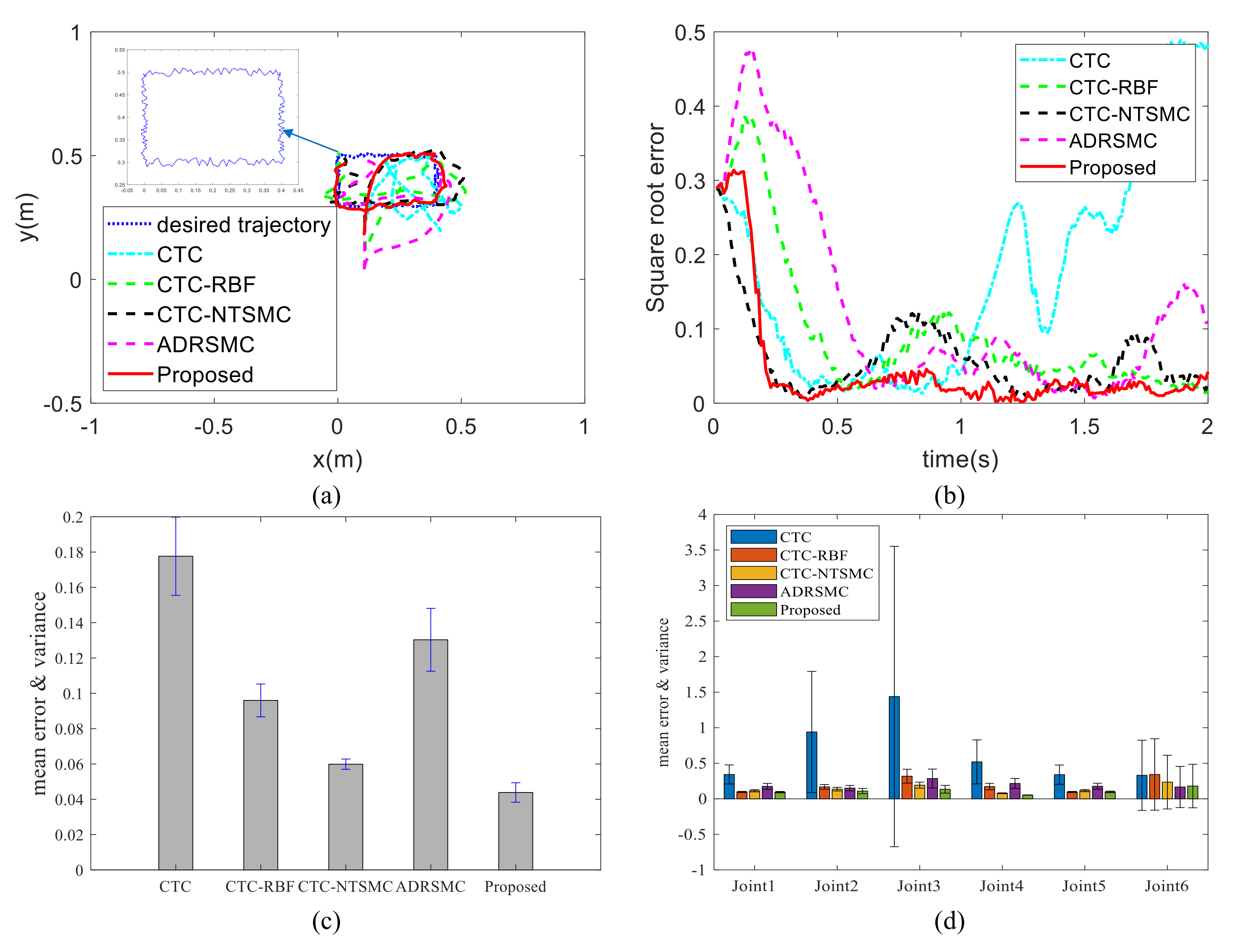
In this study, a maneuvering tele-aiming control strategy is proposed based on a novel multiple-model augmented-state extended Kalman observer (MEKO) and an active disturbance rejection terminal sliding mode controller. The control strategy enables the ground reconnaissance robot to efficiently track the maneuvering trajectory generated by the HCI device even when the robot is accompanied by joint measurement noises. To this end, a novel multiple-model observer is designed, capable of filtering the joint measurement noises and estimating the lumped disturbance simultaneously. Subsequently, a nonsingular terminal sliding mode controller is exploited to eliminate the lumped disturbance and control the robot, as an attempt to efficiently track the maneuvering trajectory. To simulate the maneuvering guidance trajectory, random offset noises are added to the guidance trajectory in the experimental verification part. To simulate the tele-aiming control system of the real robot, some random joint measurement noises are introduced when reading the joint angle. As revealed from the experiment results, the control strategy proposed in this study can endow the robot with the ability to track the maneuvering target stably under the maneuvering tele-aiming control.

Our proposed control method has a wide application background, especially in the field of robot control where the desired trajectory cannot be given in advance, such as in the field of HCI-based robot teleoperation control (ground reconnaissance robots, space manipulators, etc.). If the human traction to the robot is regarded as an external disturbance, our proposed method can also be used to the drag teaching robots.

The basic idea of MEKO is to automatically adjust the weight of each observer through the innovation covariance. Based on this idea, MEKO can output the optimal observation values of disturbance noise with different statistical characteristics in real-time, but MEKO needs to preset the process noise statistical characteristic matrix of each observer, the number of observers, and the length of the innovation sliding window. Therefore, to make up for this deficiency, our follow-up work is to explore the use of heuristic methods to automatically optimize these super parameters.

References

1. Yoon, H.U.; Lee, D. Subplanner Algorithm to Escape from Local Minima for Artificial Potential Function Based Robotic Path Planning. Int. J. Fuzzy Log. Intell. Syst. 2018, 18, 263–275. [Google Scholar] [CrossRef]
2. Shang, W.; Cong, S. Nonlinear computed torque control for a high-speed planar parallel manipulator. Mechatronics 2009, 19, 987–992. [Google Scholar] [CrossRef]
3. Lin, F.; Brandt, R.D. An Optimal Control Approach to Robust Control of Robot Manipulators. IEEE Trans. Robot. Automat. 1998, 14, 69–77. [Google Scholar]
4. Pan, H.; Xin, M. Nonlinear robust and optimal control of robot manipulators. Nonlinear Dynam. 2014, 76, 237–254. [Google Scholar] [CrossRef]
5. Ajwad, S.A.; Iqbal, J.; Islam, R.U.; Alsheikhy, A.; Almeshal, A.; Mehmood, A. Optimal and Robust Control of Multi DOF Robotic Manipulator: Design and Hardware Realization. Cybernet. Syst. 2018, 49, 77–93. [Google Scholar] [CrossRef]
6. Wang, Y.; Boyd, S. Fast Model Predictive Control Using Online Optimization. IEEE Trans. Control Syst.Technol. 2010, 18, 267–278. [Google Scholar] [CrossRef] [Green Version]
7. Cong, S.; Liang, C. Research on trajectory tracking control of 7-DOF picking manipulator. Sci. Prog. 2021, 104, 1–14. [Google Scholar] [CrossRef] [PubMed]
8. Precup, R.E.; Preitl, S.; Tar, J.K.; Tomescu, M.L.; Takacs, M.; Korondi, P.; Baranyi, P. Fuzzy Control System Performance Enhancement by Iterative Learning Control. IEEE Trans. Ind. Electron. 2008, 55, 3461–3475. [Google Scholar] [CrossRef]
9. Zhao, D.; Li, S.; Gao, F. A new terminal sliding mode control for robotic manipulators. Int. J. Control. 2009, 82, 1804–1813. [Google Scholar] [CrossRef]
10. Durmuş, B.; Temurtaş, H.; Yumuşak, N.; Temurtaş, F. A study on industrial robotic manipulator model using model based predictive controls. J. Intell. Manuf. 2009, 20, 233–241. [Google Scholar] [CrossRef]
11. Kim, J.W.; Park, B.J.; Yoo, H.; Oh, T.H.; Lee, J.H.; Lee, J.M. A model-based deep reinforcement learning method applied to finite-horizon optimal control of nonlinear control-affine system. J. Process. Control 2020, 87, 166–178. [Google Scholar] [CrossRef]
12. Li, Z.; Deng, J.; Lu, R.; Xu, Y.; Bai, J.; Su, C. Trajectory-Tracking Control of Mobile Robot Systems Incorporating Neural-Dynamic Optimized Model Predictive Approach. IEEE Trans. Syst. Man Cybernet. Syst. 2016, 46, 740–749. [Google Scholar] [CrossRef]
13. Nubert, J.; Kohler, J.; Berenz, V.; Allgower, F.; Trimpe, S. Safe and Fast Tracking on a Robot Manipulator: Robust MPC and Neural Network Control. IEEE Robot. Automat. Lett. 2020, 5, 3050–3057. [Google Scholar] [CrossRef] [Green Version]
14. Carron, A.; Arcari, E.; Wermelinger, M.; Hewing, L.; Hutter, M.; Zeilinger, M.N. Data-Driven Model Predictive Control for Trajectory Tracking With a Robotic Arm. IEEE Robot. Automat. Lett. 2019, 4, 3758–3765. [Google Scholar] [CrossRef] [Green Version]
15. Bingül, Z.; Karahan, O. A Fuzzy Logic Controller tuned with PSO for 2 DOF robot trajectory control. Expert Syst. Appl. 2011, 38, 1017–1031. [Google Scholar] [CrossRef]
16. Zhang, H.; Li, W. Tracking control using hierarchical fuzzy-regulated optimal approach for robotic manipulators. Proc. Inst. Mech. Eng. Part C J. Mech. Eng. Sci. 2018, 233, 635–648. [Google Scholar] [CrossRef]
17. Li, M.; Li, Y.; Ge, S.S.; Lee, T.H. Adaptive control of robotic manipulators with unified motion constraints. IEEE Trans. Syst. Man Cybernet. Syst. 2016, 47, 184–194. [Google Scholar] [CrossRef] [Green Version]
18. Figueredo, L.F.D.C.; Adorno, B.V.; Ishihara, J.Y. Robust H kinematic control of manipulator robots using dual quaternion algebra. Automatica 2021, 132, 109817. [Google Scholar] [CrossRef]
19. Zhai, J.; Xu, G. A Novel Non-Singular Terminal Sliding Mode Trajectory Tracking Control for Robotic Manipulators. IEEE Trans. Circuits Syst. Express Briefs 2021, 68, 391–395. [Google Scholar] [CrossRef]
20. Yang, L.; Yang, J. Nonsingular fast terminal sliding-mode control for nonlinear dynamical systems. Int. J. Robust Nonlinear Control. 2011, 21, 1865–1879. [Google Scholar] [CrossRef]
21. Nguyen, V.; Vo, A.; Kang, H. A Non-Singular Fast Terminal Sliding Mode Control Based on Third-Order Sliding Mode Observer for a Class of Second-Order Uncertain Nonlinear Systems and its Application to Robot Manipulators. IEEE Access 2020, 8, 78109–78120. [Google Scholar] [CrossRef]
22. Liu, H.; Sun, J.; Nie, J.; Zou, L. Observer-based adaptive second-order non-singular fast terminal sliding mode controller for robotic manipulators. Asian J. Control. 2020, 23, 1845–1854. [Google Scholar] [CrossRef]
23. Truong, T.N.; Vo, A.T.; Kang, H. A Backstepping Global Fast Terminal Sliding Mode Control for Trajectory Tracking Control of Industrial Robotic Manipulators. IEEE Access 2021, 9, 31921–31931. [Google Scholar] [CrossRef]
24. Chen, Y.; Ma, G.; Lin, S.; Gao, J. Adaptive Fuzzy Computed-Torque Control for Robot Manipulator with Uncertain Dynamics. Int. J. Adv. Robot. Syst. 2012, 9, 1–9. [Google Scholar] [CrossRef]
25. Chen, C.; Zhang, C.; Hu, T.; Ni, H.; Luo, W. Model-assisted extended state observer-based computed torque control for trajectory tracking of uncertain robotic manipulator systems. Int. J. Adv. Robot. Syst. 2018, 15, 1–12. [Google Scholar] [CrossRef] [Green Version]
26. WANG, L.; ZHOU, X.; HU, T. A New Computed Torque Control System with an Uncertain RBF Neural Network Controller for a 7-DOF Robot. Tehnicki Vjesnik Tech. Gazette 2020, 27, 1492–1500. [Google Scholar]
27. Yi, Y.; Fan, X.X.; Zhang, T.P. Anti-disturbance tracking control for systems with nonlinear disturbances using T–S fuzzy modeling. Neurocomputing 2016, 171, 1027–1037. [Google Scholar] [CrossRef]
28. Dong, S.; Chen, C.L.P.; Fang, M.; Wu, Z. Dissipativity-Based Asynchronous Fuzzy Sliding Mode Control for T–S Fuzzy Hidden Markov Jump Systems. IEEE Trans. Cybernet. 2020, 50, 4020–4030. [Google Scholar] [CrossRef]
29. Wu, G.; Xie, Z.; Guo, C.; Liu, H. Kalman smoothing with soft inequality constraints for space robot teleoperation. Int. J. Adv. Robot. Syst. 2018, 15, 1–12. [Google Scholar] [CrossRef] [Green Version]
30. Han, J. From PID to Active Disturbance Rejection Control. IEEE Trans. Industr. Electron. 2009, 56, 900–906. [Google Scholar] [CrossRef]
31. Liu, D.; Gao, Q.; Chen, Z.; Liu, Z. Linear Active Disturbance Rejection Control of a Two-Degrees-of-Freedom Manipulator. Math. Probl. Eng. 2020, 1–19. [Google Scholar] [CrossRef]
32. Cheng, X.; Tu, X.; Zhou, Y.; Zhou, R. Active Disturbance Rejection Control of Multi-Joint Industrial Robots Based on Dynamic Feedforward. Electronics 2019, 8, 591. [Google Scholar] [CrossRef] [Green Version]
33. Castañeda, L.A.; Luviano-Juárez, A.; Ochoa-Ortega, G.; Chairez, I. Tracking control of uncertain time delay systems: An ADRC approach. Control. Eng. Pract. 2018, 78, 97–104. [Google Scholar] [CrossRef]
34. Yao, J.; Deng, W. Active disturbance rejection adaptive control of uncertain nonlinear systems: Theory and application. Nonlinear Dyn. 2017, 89, 1611–1624. [Google Scholar] [CrossRef]
35. Shi, D.; Zhang, J.; Sun, Z.; Shen, G.; Xia, Y. Composite trajectory tracking control for robot manipulator with active disturbance rejection. Control. Eng. Pract. 2021, 106, 104670. [Google Scholar] [CrossRef]
36. Fareh, R.; Al-Shabi, M.; Bettayeb, M.; Ghommam, J. Robust Active Disturbance Rejection Control For Flexible Link Manipulator. Robotica 2020, 38, 118–135. [Google Scholar] [CrossRef]
37. Lakomy, K.; Madonski, R.; Dai, B.; Yang, J.; Kicki, P.; Ansari, M.; Li, S. Active Disturbance Rejection Control Design With Suppression of Sensor Noise Effects in Application to DC–DC Buck Power Converter. Eee Trans. Ind. Electron. 2022, 69, 816–824. [Google Scholar] [CrossRef]
38. Boutayeb, M.; Rafaralahy, H.; Darouach, M. Convergence analysis of the extended Kalman filter used as an observer for nonlinear deterministic discrete-time systems. IEEE Trans. Autom. Control 1997, 42, 581–586. [Google Scholar] [CrossRef]
39. Boutayeb, M.; Aubry, D. A strong tracking extended Kalman observer for nonlinear discrete-time systems. IEEE Trans. Autom. Control 1999, 44, 1550–1556. [Google Scholar] [CrossRef]
40. Preitl, S.; Precup, R. Iterative Feedback Tuning in Fuzzy Control Systems. Theory and Applications. Acta Polytech. Hung. 2006, 3, 81–96. [Google Scholar]
41. He, Z.; Liu, C.; Zhan, Y.; Li, H.; Huang, X.; Zhang, Z. Nonsingular Fast Terminal Sliding Mode Control with Extended State Observer and Tracking Differentiator for Uncertain Nonlinear Systems. Math. Probl. Eng. 2014, 1–19. [Google Scholar] [CrossRef]
42. Dai, Y.; Yu, S.; Yan, Y. An Adaptive EKF-FMPC for the Trajectory Tracking of UVMS. IEEE J. Oceanic. Eng. 2020, 45, 699–713. [Google Scholar] [CrossRef]
43. Wang, X.; Hou, B. Trajectory tracking control of a 2-DOF manipulator using computed torque control combined with an implicit lyapunov function method. J. Mech. Sci. Technol. 2018, 32, 2803–2816. [Google Scholar] [CrossRef]
44. Feng, Y.; Yu, X.; Man, Z. Non-singular terminal sliding mode control of rigid manipulators. Automatica 2002, 38, 2159–2167. [Google Scholar] [CrossRef]
45. Van Cuong, P.; Nan, W.Y. Adaptive trajectory tracking neural network control with robust compensator for robot manipulators. Neur. Comput. Appl. 2016, 27, 525–536. [Google Scholar] [CrossRef]
46. Ji, P.; Ma, F.; Min, F. Terminal Traction Control of Teleoperation Manipulator with Random Jitter Disturbance Based on Active Disturbance Rejection Sliding Mode Control. IEEE Access 2020, 8, 220246–220262. [Google Scholar] [CrossRef]
Figure 1. Block diagram of the proposed tele-aiming robot control system.
Mathematics 10 01268 g001
Figure 2. Block diagram of the MEKOTSMC.
Mathematics 10 01268 g002
Figure 3. Block diagram of the Multiple-model augmented-state Extended Kalman Observer.
Mathematics 10 01268 g003
Figure 4. Comparison resultsof observation. (a) represents the observation result of position, velocity, and disturbance, (b) expresses the observation mean error and variance.
Mathematics 10 01268 g004
Figure 5. Structure of UR5 robot and D-H coordinate system.
Mathematics 10 01268 g005
Figure 6. Comparison results of uniform trajectory tracking. (a) end motion trajectories without the addition of joint measurement noises, (b) end motion trajectories with the addition of joint measurement noises, (c) square root errors without the addition of joint measurement noises, (d) square root errors with the addition of joint measurement noises, (e) mean errors and variances without the addition of joint measurement noises, (f) mean errors and variances with the addition of joint measurement noises.
Mathematics 10 01268 g006
Figure 7. Comparison of mean error and variance of joint position for uniform trajectory tracking. (a) the results without the addition of joint measurement noises, (b) the results with the addition of joint measurement noises.
Mathematics 10 01268 g007
Figure 8. Comparison results of the non-uniform trajectory tracking. (a) end motion trajectories without the addition of joint measurement noises, (b) end motion trajectories with the addition of joint measurement noises, (c) square root errors without the addition of joint measurement noises, (d) square root errors with the addition of joint measurement noises, (e) mean errors and variances without the addition of joint measurement noises, (f) mean errors and variances with the addition of joint measurement noises.
Mathematics 10 01268 g008
Figure 9. Comparison mean error and variance of joint position for non-uniform trajectory tracking. (a) the results without the addition of joint measurement noises, (b) the results with the addition of joint measurement noises.
Mathematics 10 01268 g009
Figure 10. Tracking and comparison results of the non-uniform rectangular trajectory with joint measurement noises. (a) end motion trajectories, (b) square root errors, (c) mean errors and variances of whole process, (d) mean errors and variances of each joint position.
Mathematics 10 01268 g010