Non-Normal Market Losses and Spatial Dependence Using Uncertainty Indices

Abstract

We analyse spatial dependence between the risks of stock markets. An alternative definition of neighbour is used and is based on a proposed exogenous criterion obtained with a dynamic Google Trends Uncertainty Index (GTUI) designed specifically for this analysis. We show the impact of systemic risk on spatial dependence related to the most significant financial crises from 2005: the Lehman Brothers bankruptcy, the sub-prime mortgage crisis, the European debt crisis, Brexit and the COVID-19 pandemic, which also affected the financial markets. The risks are measured using the monthly variance or volatility and the monthly Value-at-Risk (VaR) of the filtered losses associated with the analysed indices. Given that the analysed risk measures follow non-normal distributions and the number of neighbours changes over time, we carry out a simulation study to check how these characteristics affect the results of global and local inference using Moran’s I statistic. Lastly, we analyse the global spatial dependence between the risks of 46 stock markets and we study the local spatial dependence for 10 benchmark stock markets worldwide.

1. Introduction

Our aim is to analyse if systemic risk is reflected in an increase in the spatial dependence between market risks, i.e., whether the detrimental and/or favourable effects of systemic risk are similar between markets with certain neighbourhood characteristics related to similar economic uncertainty. In our analysis, the market risk is approximated by the variance (volatility) and by the metric given by the Value-at-Risk (VaR) associated with the potential losses of stock markets. The losses are calculated from the negative logarithm of stock returns (hereinafter log-returns) (the loss function is defined in [1]). The differences between the volatility and the VaR as measures of risk is that the former takes into account both tails of the distributions, i.e., losses at right tail and profits at left tail, while the latter focuses on the right tail of the distribution, i.e., on the losses.

The global Moran’s I statistic (see [2]) and its local version proposed by Anselin [3] allow us to carry out inference on global and local spatial dependence, respectively. Both statistics are based on the assumption that the data are normal, independent and identically distributed and they have a known asymptotic normal distribution that is used to test the positive statistical significance of the spatial dependence, understood in our case as having similar behaviour between financial markets. Regarding non-normality, Griffith [4] concludes that the assumption of normality is not essential for the asymptotic properties of the global Moran’s I statistic. However, for the local statistic, the non-normality of the data causes errors in the inference based on the normal distribution. Given that our risk data clearly have a non-normal distribution, are right skewed and have extreme values, a simulation study is carried out to check how the global and local inference on spatial dependence is affected. The simulation study provides new results regarding the global Moran’s I test based on normal distribution when the data have heavy-tailed distribution, i.e., the study proves that spatial econometrics can be applied to the special nature of financial data.

Various studies have used bootstrap inference for testing global spatial dependence. In relation to the analysis that we present here, we highlight some studies that give robustness to our results. For example, in a regression context Yang [5] studied the consistency of the inference through a set of LM (Lagrange Multiplier) statistics using the residual-based bootstrap methods for testing spatial dependence, a special case being the global Moran’s I statistic used in this study. This author proves the consistency theoretically as well as through a simulation study where results are obtained for normal, normal mixture and log-normal. Jin and Lee [6] also analysed the consistency of bootstrap inference of global Moran’s I statistic in the spatial econometric model context and carried out a simulation study for normal and chi-square distributions. Focusing on local spatial dependence, Mei et al. [7] proposed a bootstrap method to approximate the distribution under the null hypothesis of the local Moran statistic proposed by Anselin [3]. These authors demonstrate that the asymptotic normal approximation sometimes fails.

Another important consideration of this article is the definition of neighbourhood between financial markets. Geographical distances have been the most widely used measure for calculating the spatial dependence between regions but, as shown by Acuna et al. [8], this criterion is not valid for determining the neighbours of each stock market. An alternative criterion consists of using the number of overlapping operating hours of stock markets as a measure of trading synchronisation, as proposed by Flavin et al. [9] as a proxy for the ease of trading. Acuna et al. [8] showed that overlapping operating hours criterion improves the spatial dependence results obtained using geographical distances. However, the latter is a static criterion and it is conceivable that, when the evolution of financial markets is analysed, the neighbours may change over time depending on the expectations and on the positioning of investors. For this reason, we propose the use of uncertainty indices that are exogenous to the markets themselves to give dynamism to our analysis.

Uncertainty indices have been used recently in the literature because, either through official reports or internet searches, they reflect the concerns of economic and financial agents as well as the general public about events that affect the behaviour of the country’s economy. Ahir et al. [10] obtained a quarterly index of uncertainty, called the World Economic Uncertainty Index (WUI), which was based on counting the number of times that the words “uncertainty” and its variants appeared in the Economist Intelligence Unit (EIU, https://www.eiu.com/n/) for 143 countries. These authors concluded that the level of uncertainty is significantly higher in developing countries, and it is positively associated with economic policy uncertainty and stock market volatility and negatively with GDP growth. Baker et al. [11] calculated a monthly index of Global Economic Policy Uncertainty (GEPU) that was based on the raw count of terms in three categories (economy, policy and uncertainty) divided by the total number of articles in the newspapers of 16 countries that included these terms, the searches being done in the respective native language. Using a similar process, Ghirelli et al. [12] obtained their specific Uncertainty Index for Spain. By using the Google Trends tool, Weinberg [13] proposed an Economic Policy Uncertainty Index for the largest economies in the European Union (Germany, France, Italy and Spain). Previously, Castelnuovo and Tran [14] obtained an economic Google Trend Uncertainty Index for the United States and Australia.

In this study, we use an ad-hoc Google Trend Uncertainty Index (GTUI) to select the monthly neighbours of the 46 stock indices and to carry out the spatial dependence analysis. First, we use the global Moran’s I statistic to analyse the changes of spatial dependence between stock markets. Second, we carry out a local spatial dependence, focusing on the following countries: Spain, Germany, France, Italy, UK, US, Argentina, Brazil, Japan and Hong Kong. In both analyses we identify the months with significant spatial dependence throughout the analysed period and study if during the financial crisis periods of the Lehman Brothers bankruptcy, the US sub-prime mortgage crisis, the European debt crisis, Brexit and the COVID-19 pandemic spatial dependence was more frequent compared to non-crisis periods. The proposed global spatial dependence index is an indicator of market linkages; taking this into account, our analysis answers the following three questions:

• Are months with risk positive spatial dependence during financial crisis periods more frequent than during the non-financial crisis period?
• Is positive spatial dependence just as common in all periods of crisis?
• Are there differences between volatilities with positive spatial dependence and VaRs with positive spatial dependence?

Furthermore, the analysis of local spatial dependence allows one to determine which countries have more weight in contagions during the analysed period and, therefore, which countries are the causes of them.

There are many studies that analyse market linkages, in terms of contagion effects between markets and during crisis periods, using different statistic methodologies. Below, we summarise some examples in relation to the markets that are studied in this article. Related to the global financial crisis, Dimitriou et al. [15] used a multivariate time series model for the mean, variance and correlation of log-returns called “Multivariate AR(1)-FIAPARCH-DCC process” (FIAPARCH-fractionally integrated asymmetric power ARCH and DCC-dynamic conditional correlation) to investigate the contagion effects between the five largest emerging equity markets: Brazil, Russia, India, China and South Africa (BRICS) and the US, through different phases of the crisis, and they conclude that this contagion is increased from early 2009 onwards and is greater during bull periods. In Lien et al. [16], the indirect effects of volatility between the stock markets of the US and eight East Asian countries were analysed before and during the Asian currency crisis and the sub-prime credit crisis. Among other results, these authors show how the US market is the transmitter and its volatility spills over to other markets during both crisis periods. However, between the East Asian countries, Japan and Hong Kong are markets in which volatility spills over from multiple markets during the sub-prime credit crisis period but not during the Asian currency crisis. Mohti et al. [17] used copula models that were fitted to the ARMA-GARCH filtered log-returns to investigate the contagion effects of the sub-prime financial crisis in 18 frontier markets; in relation to countries analysed in this article, these authors found that for the US and Argentina the effects were more pronounced during booms than during busts. Tilfani et al. [18], using log-returns, analysed the time cross-correlations between the US and eight other stock markets (the rest of the G7 plus China and Russia) before, during and after the financial crisis (2007–2008) and found, among other results, that in the period immediately before the crisis the levels of correlation with the US stock market increased, which could be understood as an overheating of the markets or perhaps an increase in contagion due to systemic risk. After the crisis, the results point to a contagion effect. The effect of the European debt crisis on different stock markets around the word was analysed by Samarakoon [19], who showed that the Asian markets do not present pervasive evidence of contagion from the European debt crisis (see [20] for an analysis on the European economy).

In relation to the impact of Brexit, Breinlich et al. [21] used the abnormal returns to analyse the stock market reaction to the outcome of the 2016 UK referendum on EU membership and showed that the impact would depend on the nature of post-Brexit UK-EU relations. Alternatively, using the log-returns data, Ameur and Louhichi [22] analysed the impact of Brexit on the dependency between UK, France and Germany stock markets and found that volatility and the total spillover effects increased in line with Brexit press releases regarding negotiations on the future relationship between the EU and the UK. A similar analysis is presented in Li [23] in which Italy, Poland and Ireland are also included. Burdekin et al. [24] presented an extended analysis of the Brexit effect, worldwide, using an econometric model based on log-return and abnormal log-returns to quantify the negative impact of Brexit on different stock markets. Their results showed that the Eurozone was the hardest hit, and the impact was felt the most by the so-called PIIGS group (Portugal, Ireland, Italy, Greece and Spain) due to their poor fiscal positions. On the contrary, the BRICS nations (Brazil, Russia, India, China and South Africa) fared much better than average, experiencing positive abnormal returns despite negative gross returns. In addition to these studies, it is clear that the subsequent COVID-19 pandemic has affected the development of events and has made it difficult to analyse the final effect of Brexit on financial markets.

More recently, various studies have analysed the impact of the COVID-19 pandemic on financial markets. For example, Chopra and Mehta [25] used a multivariate DCC-GARCH model of log-returns to compare the presence of contagion for the Asian stock markets during the four main financial crises: the Asian financial crisis, the US sub-prime crisis, the Eurozone debt crisis and the COVID-19 pandemic. The results showed that the US sub-prime crisis was the most contagious for the Asian stock markets, while the impact of the COVID-19 pandemic was the least contagious. Li et al. [26] investigated whether the uncertainty index proposed by Baker et al. [27], referred to as IDEMV (Infectious Disease Equity Market Volatility), had additional predictive power for stock market volatility in France, Germany and the UK during the COVID-19 pandemic. The results showed that the IDEMV had stronger predictive power for French and UK stock market volatility during the COVID-19 pandemic; however, the VIX (Volatility Index) had superior predictive power for the three European stock markets. Using a VARMA(1,1)-DCC-GARCH model for the log-return, Akhtaruzzaman et al. [28] analysed the financial contagion between China and the G7 countries. The results showed that China and Japan appeared to be transmitters during the COVID-19 pandemic.

In general, the studies that have analysed the contagion between financial markets used alternative multivariate time series models with log-returns series. In this study, we present an alternative analysis focused on the risk and use spatial dependence statistics to analyse linkages between the financial market’s volatility and its VaR metric, considering distances between the markets uncertainty levels measured by the GTUI instead of geographical distances.

The remainder of the study is organised as follows. Section 2 presents the procedure to test global and spatial dependence using asymptotic normal distribution and the bootstrap method. In Section 3, the results of a simulation study are presented that compare the asymptotic inference with bootstrap inference carried out with the global Moran’s I statistic and local Moran statistic and assuming different distributions. In Section 4, we describe the data and the spatial dependence results. In Section 5, we summarise the main conclusions.

2. The Spatial Dependence Model and Statistics for Testing

Let ${\mathbf{Y}}_t={(Y_{1t},\dots ,Y_{nt})}^{\prime }$ be a vector with data of n countries at period $t=1,\dots ,T$. It is assumed that ${\mathbf{Y}}_1,\dots ,{\mathbf{Y}}_T$ are independent and identically distributed (iid). The spatial autoregressive (SAR) model at period t is defined as:

$${\mathbf{Y}}_t={\mu }_t+{\rho }_t{W}_t{\mathbf{Y}}_t+{ϵ}_t,$$

(1)

where ${\mu }_t$ is a vector with deterministic means that can be estimated separately, ${\rho }_t$ is the spatial autocorrelation at period t and ${ϵ}_t$ is a vector with n Normal iid errors with mean 0 and variance ${\sigma }_{{ϵ}_t}^2$. The weights matrix at period t, $W_t$, is $n\times n$ and identifies the neighbours for each $i=1,\dots ,n$. In financial analysis, a fundamental component of the model defined in (1) is the weights matrix $W_t$, given that the geographical distance criterion does not work. So, a specific dynamic criteria based on internet searches from economic agents is defined.

2.1. Google Trends Uncertainty Index

Google Trends is a Google Lab that uses the Google search engine to find information related to the frequency with which a search for a particular term is carried out in various regions of the world and in various languages. The available monthly data range is from 2004 to present.

The GTUI is based on the idea that economic agents, represented by internet users, search for information online when they are not sure. This implies that the frequency of searching for terms that may be associated with future and possible bad events is high when the level of uncertainty is high. To obtain the specific index for each country, we select a broad set of keywords that are often cited in the Federal Reserve Beige Book for the US and the Reserve Bank Statement on Monetary Policy. English is chosen as the common language since it is the mostly widely used in the world. A total of 10 economic terms of interest are selected: “austerity”, “bankruptcy”, “dollar”, “financial crisis”, “recession”, “risk”, “stock exchange”, “share price”, “stock market” and “uncertainty”. These terms are related to financial markets and the crisis events that have occurred in recent years and the Google Trends tool enables us to find the frequency of searches using each of them by country and month.

We selected the 10 economic terms mentioned above based on the dictionary proposed by Castelnuovo and Tran [14]. Others studies that used similar indices are Weinberg [13] and Baker et al. [11]. The selected words are the most common among the dictionaries proposed for each measure of uncertainty mentioned by the previous authors, since these are the words that best reflect the interest of the internet users in response to an important economic world event.

Let $f_{hit}$ be the frequency of terms h in country i at period t, so the uncertainty index is defined as:

$$GTU{I}_{it}=\sum _{h=1}^{10}{f}_{hit}.$$

(2)

It must be remembered that the vocabulary determines the construction of the uncertainty index.

2.2. Weights Matrix Definition

To calculate the elements of $W_t$ we use the criteria defined by Asgharian et al. [29] based on constructing a contiguity matrix $C_t$ between markets. This matrix indicates how contiguous market i to market j is at period t, according to a measure of distance (or similarity) between both countries. We then define the matrix $C_t$ using the following distance criterion between uncertainty index values:

$$D_{ijt}=|GTU{I}_{it}-GTU{I}_{jt}|,\forall i\ne jt=1,\dots ,T.$$

(3)

Let $C_{ijt}$ be the element of $C_t$ that is the contiguity measure between country i (row) and country j (column), which is given by:

$$\begin{array}{c}\hfill C_{ijt}=1-\frac{D_{ijt}-{\min }_j{D}_{ijt}}{{\max }_j{D}_{ijt}-{\min }_j{D}_{ijt}}\forall i\ne jt=1,\dots ,T.\end{array}$$

This definition of contiguity ensures that all elements of $C_t$ lie between 0 and 1; if $C_{ijt}$ is near 0 the longest distance is from country i to country j and if $C_{ijt}$ is near 1 the shortest distance is between country i and country j. Moreover, $C_{ijt}$ is not necessarily symmetric (i.e., $C_{ijt}\ne C_{jit}$); it could be that country j is an important neighbour for country i (i.e., $C_{ijt}$ is close to 1) but country i may be unimportant for country j (i.e., $C_{ijt}$ is close to 0). The linkages matrix or spatial weights in the matrices $W_t$ are obtained from $C_{ijt}$ through row standardisation. By construction, there are zeros on the diagonal of $W_t$; a market cannot be a neighbour to itself. Then:

$$W_{ijt}=\frac{C_{ijt}}{{\sum }_{j=1}^n{C}_{ijt}},\forall i\ne jt=1,\dots ,T,$$

(4)

such that, for each row i, ${\sum }_{j=1}^n{W}_{ijt}=1$.

In order to determine with more precision which markets are neighbours, the continuity matrix is discretised, i.e., values 0 or 1 are assigned based on whether two elements are considered neighbours or not. The criterion can be based on a value c of the continuity matrix C, for example, c can be equal to the median or to a quantile. Let $C_t^{*}$ be the discretised continuity matrix, so $C_{ijt}^{*}=1$ if $C_{ijt}\ge c$ and $C_{ijt}^{*}=0$ to the contrary. In practice, the weight matrix is obtained from the row standardisation of $C_t^{*}$.

Taking into account that the sum of the rows of $C_t^{*}$ is the number of neighbours $n_{it}$ for each market, each row in the weight matrix has an element equal to $\frac{1}{n_{it}}$ or 0. Considering the SAR model defined in (1), the coefficients associated with the neighbours of the market i are ${\rho }_t\frac{1}{n_{it}}$. Therefore, the larger the number of neighbours is, the weaker the spatial dependency relation between markets.

2.3. Global Moran’s I Statistic

The Moran’s I statistic at period t is defined as the following, see [2]:

$$I_t=\frac{n}{S_{0t}}\frac{{\sum }_{i=1}^n{\sum }_{j=1}^n{W}_{ijt}\left(Y_{it}-\overline{Y_t}\right)\left(Y_{jt}-{\overline{Y}}_t\right)}{{\sum }_{i=1}^n{\left(Y_{it}-{\overline{Y}}_t\right)}^2},$$

(5)

where $\overline{Y_t}$ is the sample mean and $S_{0t}={\sum }_{i=1}^n{\sum }_{j=1}^n{W}_{ijt}$. Note that for standardised row weight matrix $S_{0t}=n$. Hereafter, the sub-index t is eliminated to simplify notation. Using matrix notation:

$$I=\frac{n}{S_{0t}}\frac{{\tilde{\mathbf{Y}}}^{\prime }W\tilde{\mathbf{Y}}}{{\tilde{\mathbf{Y}}}^{\prime }\tilde{\mathbf{Y}}},$$

(6)

where $\tilde{\mathbf{Y}}=\mathbf{Y}-\overline{\mathbf{Y}}\mathbf{1}$${}_n$ is a column vector with the n centred data, where ${\mathbf{1}}_n$ is a column vector with n ones. The asymptotic distribution of Moran’s I statistic is normal. Under the no spatial autocorrelation null hypothesis, the expectation is:

$$E\left(I\right)=-\frac{1}{n-1}.$$

(7)

The variance can be calculated under normality assumption and under unknown distribution. For the former, the result is:

$$V_N\left(I\right)=\frac{1}{(n-1)(n+1)S_0^2}(n^2{S}_1-n{S}_2+3S_0^2)-{\left(E\left(I\right)\right)}^2$$

(8)

and for the latter it is:

$$V\left(I\right)=\frac{n\left[\left(n^2-3n+3\right)S_1-n{S}_2+3S_0^2\right]-k\left[\left(n^2-n\right)S_1-2n{S}_2+6S_0^2\right]}{{(n-1)}^{\left(3\right)}{S}_0^2}-{\left(E\left(I\right)\right)}^2,$$

(9)

where k is the sample kurtosis coefficient, $S_1=\frac{1}{2}{\sum }_{i=1}^n{\sum }_{j=1}^n{\left(W_{ij}+W_{ji}\right)}^2$,

$$S_2=\frac{1}{2}\sum _{i=1}^n\sum _{j=1}^n{\left(\sum _{j=1}^n{W}_{ij}+\sum _{j=1}^n{W}_{ji}\right)}^2$$

and ${\left(A\right)}^{\left(b\right)}=A(A-1)\dots (A-b+1)$.

The inference suggested by the global Moran’s I statistic is based on the assumption that the data are independent and identically distributed (iid).

Inference on positive global spatial dependence can be based on the statistic $Z_I=\frac{I-E\left(I\right)}{V\left(I\right)}\sim Normal(0,1)$, for a given significance level p, which is a value near 0; the null hypothesis of no spatial dependence is rejected if $P(Z>Z_I)\le p$, where Z is a standard normal random variable.

Regarding non-normality, Griffith [4] concluded that this is not essential for the asymptotic properties of the Moran’s I statistic. So, the inference based on the asymptotic normal distribution of the global Moran’s I statistic works. We analyse to what extent this property is true by comparing normal based inference with the non-parametric inference based on bootstrap samples. Let ${\tilde{\mathbf{Y}}}_{\left(1\right)}^{*},\dots ,{\tilde{\mathbf{Y}}}_{\left(B\right)}^{*}$ be a set of B bootstrap random samples of size n that are selected with replacement. For each bootstrap sample, the Moran’s I statistic is calculated as:

$$I_{\left(l\right)}^{*}=\frac{n}{S_0}\frac{{\tilde{\mathbf{Y}}}_{\left(l\right)}^{*{}^{\prime }}W{\tilde{\mathbf{Y}}}_{\left(l\right)}^{*}}{{\tilde{\mathbf{Y}}}_{\left(l\right)}^{*{}^{\prime }}{\tilde{\mathbf{Y}}}_{\left(l\right)}^{*}},l=1,\dots ,B.$$

(10)

The inference on positive global spatial dependence can be based on the empirical distribution of bootstrap samples; the null hypothesis of no spatial dependence is rejected if $\frac{{\sum }_{l=1}^{B}i\left(I_{\left(l\right)}^{*}>I\right)}{B}\le p$, where $i\left(a\right)=1$ if condition a between parentheses is true. Jin and Lee [6] proved the consistency of bootstrap inference based on Moran’s I statistic.

2.4. Testing Local Spatial Dependence

The global spatial dependence analysis indicates whether there are linkages between all markets, or not, but it does not allow us to identify which markets are linked or which have spatial dependence with their neighbours and, therefore, which are linked in terms of similar risk. With the aim of analysing the local spatial dependence we use the local Moran test proposed by Anselin [3], defined as:

$$I_i=\frac{n\left(Y_i-\overline{Y}\right)}{{\sum }_{i=1}^n{\left(Y_i-\overline{Y}\right)}^2}\sum _{j=1}^n{W}_{ij}\left(Y_j-\overline{Y}\right).$$

(11)

Note that $I={\sum }_{i=1}^n{I}_i$. The expectation of local Moran statistic is:

$$E\left(I_i\right)=-\frac{W_i}{n-1},$$

(12)

where $W_i={\sum }_{j=1}^n{W}_{ij}$. The variance is:

$$V\left(I_i\right)=\frac{W_i^{\left(2\right)}\left(n-k\right)}{n-1}+\frac{2W_i^{\left(hm\right)}\left(2k-n\right)}{(n-1)(n-2)}-{\left(E\left(I_i\right)\right)}^2,$$

(13)

where $W_i^{\left(2\right)}={\sum }_{i\ne j}{W}_{ij}^2$ and $2W_i^{\left(hm\right)}={\sum }_{h\ne i}{\sum }_{m\ne i}{W}_{ih}{W}_{im}$. Although, asymptotically the distribution of $I_i$ is normal, in practice the exact distribution of this statistic is unknown and normal based inference does not work. Furthermore, given that local inference implies carrying out multiple tests using the same sample, we will need to modify the significance level, for example, using Bonferroni correction. For a given significance level p, if the number of multiple tests are r, the true significance level will be $p/r$. Similarly to the global Moran’s I test, we compare normal inference with bootstrap inference using the B bootstrap samples defined above. Mei et al. [7] proved the consistency of bootstrap inference for local Moran statistic.

3. Simulation Study

In this section we analyse the results of the inference based on the global Moran’s I and the local Moran statistics in the finite sample. We simulate the values $C_{ij}$ of the continuity matrix to obtain the weight matrix W, and we also simulate the values of the random variable Y in the SAR model defined in (1). We obtain 1000 samples of sizes $n=50$ and $n=200$, respectively. To simulate the values in W, we analyse the behaviour of the $C_{ijt}$ used in the application presented in this article and we see that these values have a behaviour similar to a random variable with distribution $Beta(4.7,3)$. To simulate the values of the random variable Y, we use the following results from the SAR model:

$$\mathbf{Y}={\left(I_n-\rho W\right)}^{-1}\left(\mathit{\mu }+\mathit{ϵ}\right),$$

(14)

where $I_n$ is the identity matrix of order n. To generate data from (14) we assume $\mathit{\mu }=\mathbf{0}$ and the value of $\mathit{ϵ}$ are generated following alternative distributions that have different shapes and tail behaviour. These distributions are: normal with parameters $\mu =0$ and $\sigma =0.25$; a Student’s t with 3 degree of freedom, $\mu =0$ and $\sigma =\frac{0.25}{\sqrt{3}}$; a log-normal with $\mu =0$ and variance $0.5$; and a log-logistic with $\mu =0$ and variance $0.5$. Note that these distributions have alternative shapes that can be found when risk variables are analysed.The normal and the Student’s t are symmetric, the second having heavier tails than the first. The log-normal and log-logistic are right skewed and the second has a heavier right tail than the first. Furthermore, log-logistic distribution is a asymptotically Pareto-type right-tailed distribution. For each distribution, the values $\rho =0.9,0.5,0.1$ are used.

In addition to the alternative distributions, the simulation study also analyses the effect on the test results depending on the number of neighbours. With this aim, the continuity matrix is discretised using different criteria for obtaining c (remember $C_{ij}^{*}=1$ if $C_{ij}>c$ and $C_{ij}^{*}=0$ on the contrary): the median (second quartile) of the values $C_{ij}$, their quantile at $75\%$ confidence level (third quartile) and their quantile at $90\%$ confidence level. Note that a higher quantile means a smaller number of neighbours. So, spatial dependence is stronger as $\rho$ increases and the number of neighbours decreases.

In

Table 1. Simulation results for global Moran’s I statistic using asymptotic inference (N) and bootstrap inference (B), both at $5\%$ significance level.

$\mathit{\alpha }=0.1$			Normal		Student’s t		Log-Normal		Log-Logistic
n	Quantile	$\mathit{\rho }$	N	B	N	B	N	B	N	B
		0.9	0.461	0.456	0.543	0.527	0.536	0.520	0.728	0.663
	50	0.5	0.268	0.275	0.306	0.290	0.298	0.275	0.495	0.299
		0.1	0.126	0.121	0.133	0.127	0.116	0.108	0.176	0.094
		0.9	0.806	0.808	0.879	0.874	0.877	0.868	0.956	0.952
50	75	0.5	0.456	0.457	0.521	0.507	0.504	0.474	0.737	0.635
		0.1	0.133	0.131	0.155	0.149	0.151	0.140	0.228	0.108
		0.9	0.999	0.999	0.996	0.996	0.997	0.997	1.000	0.999
	90	0.5	0.815	0.813	0.850	0.846	0.858	0.844	0.957	0.936
		0.1	0.198	0.206	0.193	0.186	0.196	0.183	0.293	0.156
		0.9	0.498	0.503	0.498	0.507	0.536	0.528	0.710	0.665
	50	0.5	0.285	0.286	0.298	0.297	0.300	0.297	0.501	0.347
		0.1	0.134	0.133	0.131	0.126	0.145	0.140	0.203	0.100
		0.9	0.838	0.840	0.833	0.830	0.858	0.857	0.951	0.937
200	75	0.5	0.495	0.502	0.496	0.483	0.504	0.488	0.684	0.596
		0.1	0.141	0.143	0.160	0.154	0.162	0.157	0.222	0.104
		0.9	0.993	0.993	0.998	0.998	0.998	0.998	1.000	1.000
	90	0.5	0.842	0.844	0.818	0.814	0.829	0.820	0.961	0.952
		0.1	0.191	0.192	0.211	0.203	0.209	0.200	0.294	0.149
$\mathit{\alpha }=\mathbf{0.05}$			Normal		Student’s t		Log-Normal		Log-Logistic
n	Quantile	$\mathit{\rho }$	N	B	N	B	N	B	N	B
		0.9	0.341	0.341	0.402	0.384	0.403	0.368	0.640	0.482
	50	0.5	0.168	0.172	0.189	0.183	0.187	0.163	0.381	0.174
		0.1	0.069	0.069	0.067	0.067	0.061	0.058	0.109	0.048
		0.9	0.705	0.704	0.776	0.765	0.790	0.759	0.923	0.900
50	75	0.5	0.318	0.316	0.361	0.344	0.383	0.319	0.611	0.354
		0.1	0.075	0.077	0.087	0.078	0.093	0.074	0.161	0.050
		0.9	0.993	0.991	0.992	0.992	0.994	0.993	0.999	0.999
	90	0.5	0.711	0.708	0.760	0.740	0.758	0.705	0.887	0.787
		0.1	0.109	0.108	0.118	0.116	0.116	0.095	0.222	0.073
		0.9	0.353	0.355	0.380	0.375	0.410	0.394	0.610	0.525
	50	0.5	0.182	0.192	0.178	0.178	0.209	0.201	0.393	0.202
		0.1	0.068	0.068	0.072	0.069	0.067	0.060	0.108	0.036
		0.9	0.726	0.724	0.708	0.710	0.752	0.748	0.901	0.867
200	75	0.5	0.350	0.342	0.350	0.344	0.370	0.349	0.569	0.336
		0.1	0.086	0.087	0.084	0.085	0.096	0.088	0.158	0.052
		0.9	0.987	0.986	0.993	0.993	0.995	0.994	1.000	1.000
	90	0.5	0.987	0.986	0.709	0.700	0.750	0.728	0.892	0.817
		0.1	0.100	0.099	0.127	0.121	0.121	0.112	0.215	0.063

the results of inference at $5\%$ significance level using the global Moran’s I statistic are shown. On the 1000 replicates of each sample, we calculate the percentage of rejection of the null hypothesis of spatial independence from the alternative hypothesis of positive spatial dependence. For every replicate, the test is carried out using asymptotic inference based on normal distribution (N) and with the finite inference based on 1000 bootstrap random samples (B) with replacement and the same size of the original samples. For normal distributions, Student’s t and log-normal, the results with N and B are similar in all cases. When the spatial dependence is clear, i.e., $\rho =0.9$ and the neighbourhood criterion is based on the quantile at $90\%$ confidence level, the percentage of rejections is practically equal to 1 in all cases. When the number of neighbours increases this percentage decreases and it is similar when the value $\rho$ decreases. For the log-logistic distribution, again, the results for N and B are very similar when the neighbourhood criterion is based on the quantile at $90\%$ confidence level and $\rho =0.9$ or $\rho =0.5$. However, when the number of neighbours is at its highest and $\rho <0.9$, the percentage of rejection with N is greater than that obtained with B. Compared with the alternative distributions, for the log-logistic, which is Pareto tailed, the asymptotic inference based on Normal distribution will have larger type I error, i.e., the null hypothesis could be rejected with more probability when this is true.

Table 2. Simulation results for local Moran statistic with maximum number of neighbours using asymptotic inference (N) and bootstrap inference (B), both at $10\%$ significance level.

$\mathit{\alpha }=0.1$			Normal		Student’s t		Log-Normal		Log-Logistic
n	Quantile	$\mathit{\rho }$	N	B	N	B	N	B	N	B
		0.9	0.144	0.143	0.152	0.153	0.141	0.153	0.204	0.148
	50	0.5	0.119	0.119	0.124	0.124	0.120	0.123	0.184	0.129
		0.1	0.099	0.099	0.105	0.097	0.098	0.101	0.161	0.098
		0.9	0.181	0.186	0.217	0.204	0.190	0.193	0.229	0.175
50	75	0.5	0.132	0.140	0.157	0.156	0.137	0.139	0.141	0.139
		0.1	0.091	0.100	0.127	0.107	0.092	0.087	0.083	0.080
		0.9	0.304	0.289	0.318	0.275	0.309	0.282	0.272	0.155
	90	0.5	0.203	0.197	0.200	0.203	0.192	0.195	0.181	0.173
		0.1	0.132	0.122	0.112	0.109	0.085	0.105	0.063	0.080
		0.9	0.114	0.108	0.110	0.120	0.110	0.092	0.126	0.141
	50	0.5	0.103	0.101	0.102	0.112	0.097	0.079	0.116	0.113
		0.1	0.097	0.088	0.094	0.096	0.089	0.073	0.119	0.099
		0.9	0.134	0.131	0.132	0.137	0.122	0.136	0.163	0.137
200	75	0.5	0.114	0.108	0.113	0.117	0.100	0.115	0.102	0.116
		0.1	0.096	0.087	0.099	0.094	0.085	0.086	0.081	0.081
		0.9	0.186	0.190	0.171	0.187	0.175	0.183	0.185	0.193
	90	0.5	0.137	0.154	0.131	0.132	0.132	0.140	0.127	0.130
		0.1	0.102	0.118	0.099	0.096	0.098	0.101	0.053	0.060
$\mathit{\alpha }=\mathbf{0.05}$			Normal		Student’s t		Log-Normal		Log-Logistic
n	Quantile	$\mathit{\rho }$	N	B	N	B	N	B	N	B
		0.9	0.071	0.076	0.077	0.084	0.079	0.089	0.103	0.078
	50	0.5	0.051	0.064	0.064	0.065	0.061	0.065	0.087	0.065
		0.1	0.040	0.048	0.054	0.045	0.052	0.051	0.071	0.041
		0.9	0.108	0.111	0.125	0.116	0.101	0.109	0.106	0.102
50	75	0.5	0.059	0.078	0.089	0.078	0.064	0.065	0.062	0.070
		0.1	0.040	0.049	0.060	0.057	0.040	0.040	0.033	0.036
		0.9	0.205	0.195	0.210	0.183	0.208	0.178	0.191	0.155
	90	0.5	0.125	0.127	0.110	0.112	0.103	0.107	0.120	0.077
		0.1	0.074	0.067	0.050	0.064	0.029	0.046	0.032	0.033
		0.9	0.054	0.053	0.048	0.071	0.054	0.050	0.054	0.071
	50	0.5	0.049	0.049	0.044	0.065	0.046	0.045	0.048	0.056
		0.1	0.049	0.042	0.043	0.058	0.041	0.039	0.049	0.043
		0.9	0.066	0.075	0.066	0.075	0.072	0.081	0.062	0.069
200	75	0.5	0.054	0.060	0.060	0.061	0.053	0.067	0.039	0.055
		0.1	0.048	0.045	0.054	0.050	0.045	0.049	0.030	0.039
		0.9	0.096	0.121	0.095	0.098	0.102	0.101	0.126	0.107
	90	0.5	0.071	0.093	0.067	0.068	0.066	0.075	0.087	0.054
		0.1	0.057	0.062	0.040	0.047	0.042	0.045	0.022	0.030

,

Table 3. Simulation results for local Moran statistic with medium number of neighbours using asymptotic inference (N) and bootstrap inference (B), both at $10\%$ significance level.

$\mathit{\alpha }=0.1$			Normal		Student’s t		Log-Normal		Log-Logistic
n	Quantile	$\mathit{\rho }$	N	B	N	B	N	B	N	B
		0.9	0.148	0.170	0.166	0.161	0.153	0.161	0.169	0.160
	50	0.5	0.123	0.129	0.139	0.130	0.123	0.122	0.133	0.126
		0.1	0.103	0.098	0.114	0.106	0.100	0.090	0.099	0.084
		0.9	0.177	0.186	0.161	0.188	0.182	0.207	0.212	0.174
50	75	0.5	0.139	0.144	0.144	0.137	0.129	0.151	0.130	0.117
		0.1	0.110	0.111	0.117	0.094	0.102	0.103	0.057	0.073
		0.9	0.277	0.286	0.254	0.290	0.267	0.293	0.206	0.275
	90	0.5	0.203	0.201	0.164	0.199	0.162	0.194	0.143	0.190
		0.1	0.128	0.132	0.099	0.101	0.083	0.121	0.051	0.069
		0.9	0.118	0.128	0.105	0.112	0.128	0.139	0.112	0.129
	50	0.5	0.114	0.117	0.096	0.106	0.118	0.118	0.104	0.108
		0.1	0.105	0.105	0.092	0.092	0.113	0.105	0.104	0.078
		0.9	0.119	0.121	0.135	0.155	0.127	0.150	0.149	0.120
200	75	0.5	0.108	0.109	0.110	0.125	0.107	0.129	0.094	0.087
		0.1	0.095	0.082	0.088	0.102	0.093	0.093	0.049	0.048
		0.9	0.171	0.190	0.154	0.171	0.161	0.180	0.131	0.187
	90	0.5	0.141	0.147	0.136	0.137	0.118	0.148	0.095	0.126
		0.1	0.112	0.119	0.099	0.107	0.084	0.103	0.027	0.048
$\mathit{\alpha }=\mathbf{0.05}$			Normal		Student’s t		Log-Normal		Log-Logistic
n	Quantile	$\mathit{\rho }$	N	B	N	B	N	B	N	B
		0.9	0.081	0.095	0.091	0.091	0.083	0.087	0.070	0.090
	50	0.5	0.064	0.066	0.073	0.071	0.059	0.064	0.048	0.066
		0.1	0.048	0.051	0.055	0.051	0.041	0.050	0.034	0.042
		0.9	0.101	0.114	0.100	0.101	0.112	0.113	0.108	0.084
50	75	0.5	0.075	0.085	0.081	0.077	0.069	0.081	0.066	0.063
		0.1	0.052	0.053	0.057	0.049	0.046	0.052	0.021	0.037
		0.9	0.167	0.189	0.151	0.192	0.154	0.198	0.137	0.169
	90	0.5	0.107	0.124	0.101	0.111	0.093	0.117	0.113	0.121
		0.1	0.066	0.073	0.059	0.050	0.050	0.059	0.033	0.040
		0.9	0.064	0.063	0.047	0.057	0.064	0.070	0.046	0.070
	50	0.5	0.059	0.056	0.044	0.051	0.061	0.064	0.042	0.054
		0.1	0.053	0.045	0.042	0.043	0.059	0.048	0.037	0.034
		0.9	0.056	0.064	0.071	0.080	0.053	0.084	0.091	0.056
200	75	0.5	0.048	0.056	0.056	0.065	0.048	0.056	0.054	0.040
		0.1	0.039	0.041	0.047	0.049	0.037	0.036	0.021	0.026
		0.9	0.091	0.110	0.093	0.104	0.093	0.115	0.091	0.111
	90	0.5	0.077	0.087	0.068	0.076	0.060	0.088	0.076	0.072
		0.1	0.059	0.066	0.045	0.053	0.037	0.057	0.017	0.025

and

Table 4. Simulation results for local Moran statistic with minimum number of neighbours using asymptotic inference (N) and bootstrap inference (B), both at $10\%$ significance level.

$\mathit{\alpha }=0.1$			Normal		Student’s t		Log-Normal		Log-Logistic
n	Quantile	$\mathit{\rho }$	N	B	N	B	N	B	N	B
		0.9	0.168	0.180	0.173	0.173	0.176	0.198	0.195	0.180
	50	0.5	0.133	0.152	0.139	0.139	0.141	0.152	0.111	0.123
		0.1	0.106	0.125	0.113	0.108	0.116	0.120	0.081	0.069
		0.9	0.184	0.212	0.210	0.246	0.172	0.228	0.167	0.237
50	75	0.5	0.130	0.161	0.161	0.182	0.121	0.164	0.119	0.164
		0.1	0.094	0.110	0.121	0.110	0.075	0.107	0.041	0.056
		0.9	0.212	0.309	0.147	0.300	0.099	0.313	0.066	0.252
	90	0.5	0.175	0.224	0.125	0.209	0.078	0.222	0.064	0.156
		0.1	0.123	0.111	0.086	0.118	0.046	0.116	0.043	0.062
		0.9	0.122	0.141	0.147	0.119	0.125	0.153	0.127	0.143
	50	0.5	0.110	0.126	0.129	0.107	0.119	0.132	0.095	0.114
		0.1	0.099	0.114	0.111	0.091	0.107	0.112	0.085	0.080
		0.9	0.131	0.160	0.120	0.135	0.147	0.180	0.139	0.180
200	75	0.5	0.119	0.139	0.104	0.115	0.130	0.145	0.088	0.110
		0.1	0.105	0.122	0.091	0.094	0.110	0.114	0.033	0.055
		0.9	0.179	0.193	0.163	0.183	0.141	0.227	0.095	0.203
	90	0.5	0.145	0.155	0.128	0.138	0.100	0.162	0.077	0.141
		0.1	0.114	0.118	0.100	0.093	0.071	0.105	0.023	0.044
$\mathit{\alpha }=\mathbf{0.05}$			Normal		Student’s t		Log-Normal		Log-Logistic
n	Quantile	$\mathit{\rho }$	N	B	N	B	N	B	N	B
		0.9	0.097	0.123	0.102	0.101	0.101	0.123	0.069	0.091
	50	0.5	0.077	0.090	0.085	0.077	0.059	0.094	0.044	0.052
		0.1	0.052	0.064	0.065	0.056	0.049	0.066	0.026	0.032
		0.9	0.099	0.142	0.125	0.165	0.081	0.134	0.120	0.152
50	75	0.5	0.064	0.096	0.092	0.106	0.052	0.092	0.102	0.088
		0.1	0.043	0.062	0.068	0.067	0.033	0.050	0.028	0.029
		0.9	0.115	0.220	0.077	0.176	0.058	0.181	0.058	0.142
	90	0.5	0.082	0.134	0.077	0.134	0.055	0.124	0.053	0.088
		0.1	0.059	0.064	0.056	0.058	0.033	0.058	0.038	0.045
		0.9	0.062	0.071	0.073	0.065	0.055	0.089	0.040	0.072
	50	0.5	0.055	0.065	0.059	0.057	0.048	0.077	0.025	0.048
		0.1	0.052	0.058	0.051	0.052	0.044	0.060	0.022	0.024
		0.9	0.066	0.102	0.067	0.077	0.081	0.115	0.106	0.088
200	75	0.5	0.055	0.086	0.055	0.059	0.068	0.092	0.070	0.047
		0.1	0.045	0.071	0.052	0.046	0.055	0.072	0.016	0.026
		0.9	0.092	0.123	0.106	0.102	0.086	0.140	0.074	0.119
	90	0.5	0.072	0.088	0.076	0.076	0.054	0.083	0.068	0.085
		0.1	0.048	0.057	0.058	0.054	0.031	0.046	0.021	0.019

show the results for local spatial inference using the local Moran statistic. The results for three observations with different number of neighbours (maximum, median and minimum) are, respectively, analysed. In general, as expected, the results of local inference indicate that the percentage of rejections of the null hypothesis of spatial independence is much lower than in the global test, this finding having already been presented by Anselin [3]. However, in our simulation study we find some novel results, described below.

In the same way as for the global Moran’s I, with the local Moran statistic we also observe that as the number of neighbours increases the null hypothesis is not rejected with more frequency. Furthermore, as Table 2 shows, concerning the results for the case with the maximum number of neighbours with each criterion, by using asymptotic inference (N) we obtain a higher percentage of rejection than with bootstrap (B). In contrast, in Table 3 and Table 4, where the cases with median and minimum neighbours are analysed, respectively, the percentage of rejection tends to be the highest with B, i.e., bootstrap inference has clearly more power than asymptotic inference based on normal distribution. In other words, fewer errors are made when rejecting the null hypothesis of independence.

Analysing the results of local inference for alternative distributions, we observe that the differences between N and B are the lowest for normal and Student’s t distributions. For log-normal and log-logistic distributions the asymptotic inference barely detects spatial dependence in those cases where it could be stronger, i.e., minimum number of neighbours with neighbourhood criteria based on the quantile at $90\%$ confidence level and with $\rho =0.9$. In these cases the bootstrap inference considerably improves normal based inference.

4. Data Analysis

In our study, 45 countries and 46 stock indices (USA has two: Standard & Poor’s 500 and Dow Jones) are analysed monthly. These countries and stock indices are listed in

Table A1. Descriptive statistics of stock market losses.

Country	Label	Index	Mean	STD	Min	Median	Max	Skew	Kurtosis
Argentina	AR	MERVAL	−0.80%	4.66%	−10.66%	−0.58%	23.28%	0.952	3.988
Australia	AU	S&P-ASX200	−0.15%	1.76%	−4.12%	−0.46%	10.34%	1.467	5.467
Austria	AT	ATX	−0.15%	2.96%	−9.44%	−0.47%	14.38%	1.420	5.567
Belgium	BE	BEL20	−0.11%	2.14%	−8.10%	−0.47%	10.46%	1.155	4.372
Brazil	BR	BOVESPA	−0.34%	2.95%	−6.81%	−0.35%	15.43%	1.009	4.153
Canada	CA	S&PTSX	−0.17%	1.70%	−4.61%	−0.38%	8.48%	1.480	6.016
Chile	CL	IPSA	−0.24%	2.05%	−6.48%	−0.18%	7.27%	0.043	0.727
Czech Rep	CZ	PX	−0.10%	2.62%	−7.43%	−0.28%	13.74%	1.276	5.344
Denmark	DK	OMX	−0.37%	2.09%	−8.04%	−0.48%	9.04%	0.819	3.385
Egypt	EG	EGX 30	−0.48%	3.96%	−13.54%	−0.47%	15.05%	0.281	1.842
Finland	FI	OMXH25	−0.24%	2.27%	−9.86%	−0.47%	8.10%	0.413	2.400
France	FR	CAC40	−0.10%	2.10%	−7.96%	−0.38%	8.20%	0.535	1.768
Germany	DE	DAX	−0.27%	2.27%	−6.73%	−0.57%	9.25%	0.822	2.233
Greece	GR	ATH	0.21%	3.91%	−11.19%	−0.21%	14.19%	0.661	1.242
Hong Kong	HK	HANG SENG	−0.18%	2.54%	−6.85%	−0.52%	11.05%	0.687	1.855
Hungary	HU	BUX	−0.33%	2.83%	−7.97%	−0.52%	14.52%	0.871	3.816
Iceland	IS	ICEX	0.00%	4.64%	−7.14%	−0.43%	54.52%	8.187	90.454
India	IN	BSE SENSEX 30	−0.45%	2.82%	−10.81%	−0.50%	12.92%	0.957	4.191
Indonecia	ID	IDX	−0.47%	2.53%	−7.97%	−0.73%	16.38%	1.655	9.189
Ireland	IE	ISEQ 20	−0.09%	2.48%	−7.74%	−0.37%	10.24%	1.099	2.886
Israel	IL	TA35	−0.24%	2.04%	−4.74%	−0.47%	8.72%	0.985	2.479
Italy	IT	FTSE MIB	0.03%	2.63%	−8.97%	−0.32%	11.04%	0.500	1.908
Japan	JP	NIKKEI 225	−0.21%	2.39%	−6.09%	−0.48%	11.82%	0.902	2.505
Malaysia	MY	KLCI	−0.14%	1.51%	−5.52%	−0.28%	7.17%	0.513	2.941
Mexico	MX	IPC	−0.35%	2.09%	−5.38%	−0.39%	8.54%	0.718	2.012
Netherlands	NL	AEX	−0.14%	2.12%	−5.50%	−0.49%	9.54%	1.192	3.654
New Zeland	NZ	S&PNZX10	−0.34%	1.48%	−3.64%	−0.46%	6.05%	1.088	2.725
Norway	NO	OSEAX	−0.37%	2.42%	−6.09%	−0.60%	11.88%	1.432	5.196
Pakistan	PK	KARACHI100	−0.49%	3.09%	−8.78%	−0.79%	19.49%	1.707	8.665
Peru	PE	IGBVL	−0.47%	3.57%	−14.13%	−0.43%	20.26%	0.597	6.057
Philippines	PH	PSEI	−0.33%	2.33%	−6.06%	−0.57%	11.96%	1.192	4.825
Poland	PL	WIG20	−0.05%	2.64%	−8.18%	−0.21%	11.59%	0.455	1.706
Portugal	PT	PSI20	0.07%	2.32%	−6.71%	−0.14%	10.14%	0.714	1.893
Russia	RU	RTSI	−0.20%	4.08%	−11.59%	−0.41%	19.51%	0.815	2.730
Singapore	SG	STI	−0.11%	2.18%	−8.38%	−0.39%	11.88%	1.019	5.996
Slovakia	SK	SAX	−0.15%	2.16%	−12.63%	−0.22%	8.89%	−0.685	6.303
South Korea	KR	KOSPI200	−0.28%	2.29%	−5.80%	−0.39%	11.43%	0.743	3.155
Spain	ES	IBEX35	−0.02%	2.49%	−9.75%	−0.31%	10.91%	0.395	2.892
Sweden	SE	OMXS30	−0.25%	2.00%	−6.81%	−0.37%	8.02%	0.817	2.266
Swiss	CH	SMI	−0.14%	1.54%	−4.19%	−0.38%	5.22%	0.536	0.560
Taiwan	TW	TWII	−0.21%	2.24%	−6.07%	−0.42%	9.06%	0.689	1.876
Thailand	TH	SET	−0.14%	2.50%	−7.13%	−0.41%	15.60%	1.384	7.275
Turkey	TR	BIST100	−0.44%	3.31%	−8.94%	−0.75%	11.42%	0.417	0.500
UK	GB	FTSE100	−0.08%	1.68%	−5.06%	−0.35%	6.45%	0.730	1.604
USA	US	DOWJONES	−0.23%	1.76%	−4.86%	−0.36%	6.58%	0.806	2.064
USA	US	S&P 500	−0.26%	1.82%	−5.19%	−0.52%	8.06%	0.892	2.487

in Appendix A. Each country is labelled using the two digits notation. The frequencies of words per country and month were added to obtain our proposed GTUI. The period analysed is from January 2004 to March 2021. The four sub-periods distinguished, containing the most important financial crises in the 21st century to date, are as follows: the US sub-prime period between 31 August 2007 and 30 June 2009; the Euro debt crisis between 30 June 2010 and 30 June 2014; Brexit between 30 June 2016 and 31 January 2020; and the COVID-19 pandemic between 29 February 2020 and 31 March 2021. To obtain the results of spatial dependence, the criterion for defining the neighbours was the median. The criteria based on the most extreme quantiles used in the simulation study of Section 3 led to a very small number of neighbours, possibly even equal to zero in some periods, which causes difficulties in calculating the statistics for testing spatial dependency.

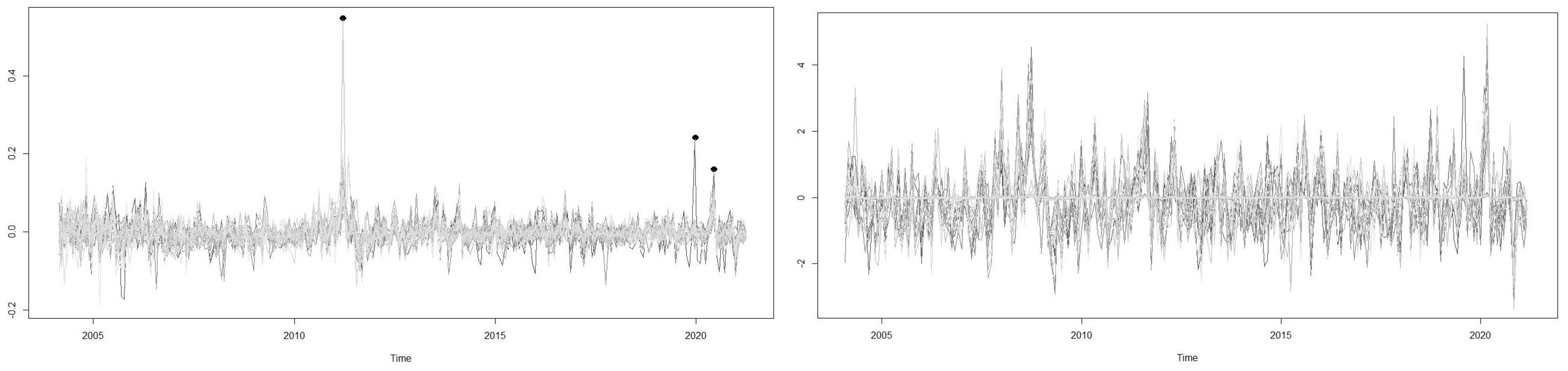
The initial data are the monthly value of market indices $M{I}_{ti}$, $t=1,\dots ,207$ and $i=1,\dots ,46$. We used monthly data because the information from Google Trends necessary for the construction of the uncertainty index is available monthly. The monthly losses are $l_{ti}=-log\left(\frac{M{I}_{ti}}{M{I}_{(t-1)i}}\right)$, where for $t=1$ we obtain the value of $t-1=0$. In total, we have 46 series of losses, described in Table A1 of Appendix A. The Shapiro–Wilk test for small samples and the Kolmogorov–Smirnov test for large samples are used to study the normality of the risk series; we omit normal inference results and for all the series the normality assumption is rejected. For each monthly loss series, we study its stationarity in mean and variance and filter the series with the fitted ARMA-GARCH models that are shown in

Table A2. Fitted ARMA-GARCH models.

Label	Index	Model
AR	MERVAL	ARMA(0, 0) - GARCH(1, 1)
AU	S&P-ASX200	ARMA(0, 0) - GARCH(1, 1)
AT	ATX	ARMA(1, 0) - GARCH(0, 0)
BE	BEL20	ARMA(1, 0) - GARCH(0, 0)
BR	BOVESPA	ARMA(0, 0) - GARCH(0, 0)
CA	S&PTSX	ARMA(0, 0) - GARCH(1, 1)
CL	IPSA	ARMA(0, 0) - GARCH(1, 1)
CZ	PX	ARMA(1, 0) - GARCH(0, 0)
DK	OMX	ARMA(1, 0) - GARCH(0, 0)
EG	EGX30	ARMA(1, 0) - GARCH(0, 0)
FI	OMXH25	ARMA(1, 0) - GARCH(0, 0)
FR	CAC40	ARMA(0, 0) - GARCH(1, 1)
DE	DAX	ARMA(0, 0) - GARCH(0, 0)
GR	ATH	ARMA(1, 0) - GARCH(0, 0)
HK	HANG SENG	ARMA(0, 0) - GARCH(1, 1)
HU	BUX	ARMA(1, 0) - GARCH(0, 0)
IS	ICEX	ARMA(1, 0) - GARCH(0, 0)
IN	BSE SENSEX30	ARMA(0, 0) - GARCH(1, 1)
ID	IDX	ARMA(1, 0) - GARCH(0, 0)
IE	ISEQ20	ARMA(1, 0) - GARCH(0, 0)
IL	TA35	ARMA(0, 0) - GARCH(1, 1)
IT	FTSE MIB	ARMA(0, 0) - GARCH(0, 0)
JP	NIKKEI225	ARMA(0, 0) - GARCH(1, 1)
MY	KLCI	ARMA(0, 0) - GARCH(0, 0)
MX	IPC	ARMA(0, 0) - GARCH(0, 0)
NL	AEX	ARMA(0, 0) - GARCH(1, 1)
NZ	S&PNZX10	ARMA(0, 0) - GARCH(0, 0)
NO	OSEAX	ARMA(1, 0) - GARCH(0, 0)
PK	KARACHI100	ARMA(0, 0) - GARCH(0, 0)
PE	IGBVL	ARMA(1, 0) - GARCH(0, 0)
PH	PSEI	ARMA(0, 0) - GARCH(0, 0)
PL	WIG20	ARMA(0, 0) - GARCH(1, 1)
PT	PSI20	ARMA(1, 0) - GARCH(0, 0)
RU	RTSI	ARMA(1, 0) - GARCH(0, 0)
SG	STI	ARMA(0, 0) - GARCH(0, 0)
SK	SAX	ARMA(1, 0) - GARCH(0, 0)
KR	KOSPI200	ARMA(0, 0) - GARCH(0. 0)
SP	IBEX35	ARMA(0, 0) - GARCH(0, 0)
SE	OMXS30	ARMA(0, 0) - GARCH(0, 0)
CH	SMI	ARMA(0, 0) - GARCH(1, 1)
TW	TWII	ARMA(1, 0) - GARCH(0, 0)
TH	SET	ARMA(1, 0) - GARCH(0, 0)
TR	BIST100	ARMA(0, 0) - GARCH(0, 0)
UK	FTSE100	ARMA(0, 0) - GARCH(1, 1)
US	DOWJONES	ARMA(0, 0) - GARCH(1, 1)
US	S&P 500	ARMA(0, 0) - GARCH(1, 1)

in Appendix A. The series of losses called $l_{ti}$ and the standardised residuals $r_{ti}$ of ARMA-GARCH models, called filtered series, are plotted in Figure 1. Three main positive peaks are prominent in the plot on the left. The first corresponds to October 2010 in the middle of the Euro debt crisis, where Iceland reached losses of more than $50\%$, followed by Peru, Argentina and Russia, whose indices lost $20\%$ of their value. The second peak is in August 2019 and corresponds to the economic crisis in Argentina, a country whose stock index lost more than $23\%$ of its value. The third is in March 2020, coinciding with the health crisis of the COVID-19 pandemic which has affected the whole world and during which, for example, Austria, Spain, Italy and Greece in the Eurozone lost more than $10\%$ of their stock index value. In the plot on the right, showing the standardised residuals of the ARMA-GARCH fitted model, the four crisis periods are reflected with greater instability in the series.

With the filtered data we estimate the monthly risk with two alternative measures, the volatility and the VaR at $99\%$ confidence level, using the rolling method with a window of 12 months. This window is selected considering that we work with long monthly series and, in addition to the volatility, where a window of 6 is very common, we must estimate the VaR at $99\%$, in this case a window of 12 provides less sensitive results. The first year of data was not available, leaving us with information for 195 months, from January 2005 to March 2021. Let $r_{it}$ be the standardised residual of stock market i and month t, the volatility is estimated with the known formula for the variance, ${\widehat{\sigma }}_{it}^2=\frac{{\sum }_{s=t-12}^t{\left(r_{is}-{\overline{r}}_{it}\right)}^2}{12}$, where ${\overline{r}}_{it}=\frac{{\sum }_{s=t-12}^t{r}_{is}}{12}$. The VaR is estimated using the formula that takes into account the deviations from the normal distribution, i.e., the modified VaR MVaR. Due to the non-normality of the data and the diversity of the 46 analysed series, parametric and Monte Carlo approaches do not make sense, the MVaR is the most consistent estimation in our case, and it is:

$$MVa{R}_{it}={\overline{l}}_{it}+Z_{CF}{\widehat{\sigma }}_{it}.$$

In the MVaR formula, the term

$$Z_{CF}=Z_{\alpha }+\frac{\left(Z_{\alpha }^2-1\right)S}{6}+\frac{\left(Z_{\alpha }^3-3Z_{\alpha }\right)K}{24}-\frac{\left(2Z_{\alpha }^3-5Z_{\alpha }\right)S^2}{36}$$

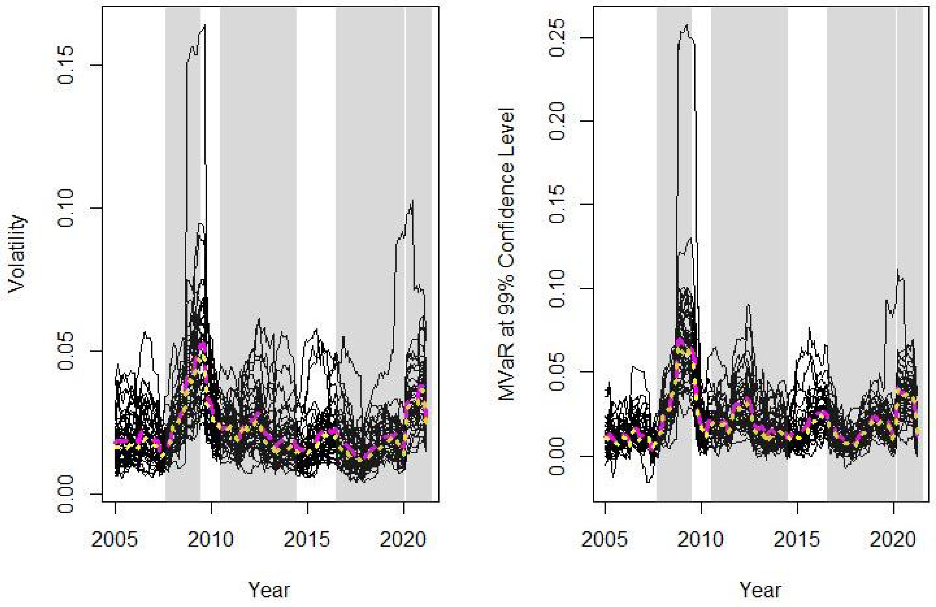
is the Cornish Fisher approximation of the $\alpha$ quantile, where S and $K=k-3$ refer to skewness and the excess of kurtosis of the data. Our variables, therefore, in formulas (5) and (11) for global and local Moran statistics are $Y_{it}={\widehat{\sigma }}_{it}^2$ and $Y_{it}=MVa{R}_{it}$. In Figure 2 both risk measures for the 46 indices are plotted, including their means (magenta long dashed line) and medians (yellow short dashed line) throughout the analysed period. In all the figures that are shown in this section, the crisis periods are shaded.

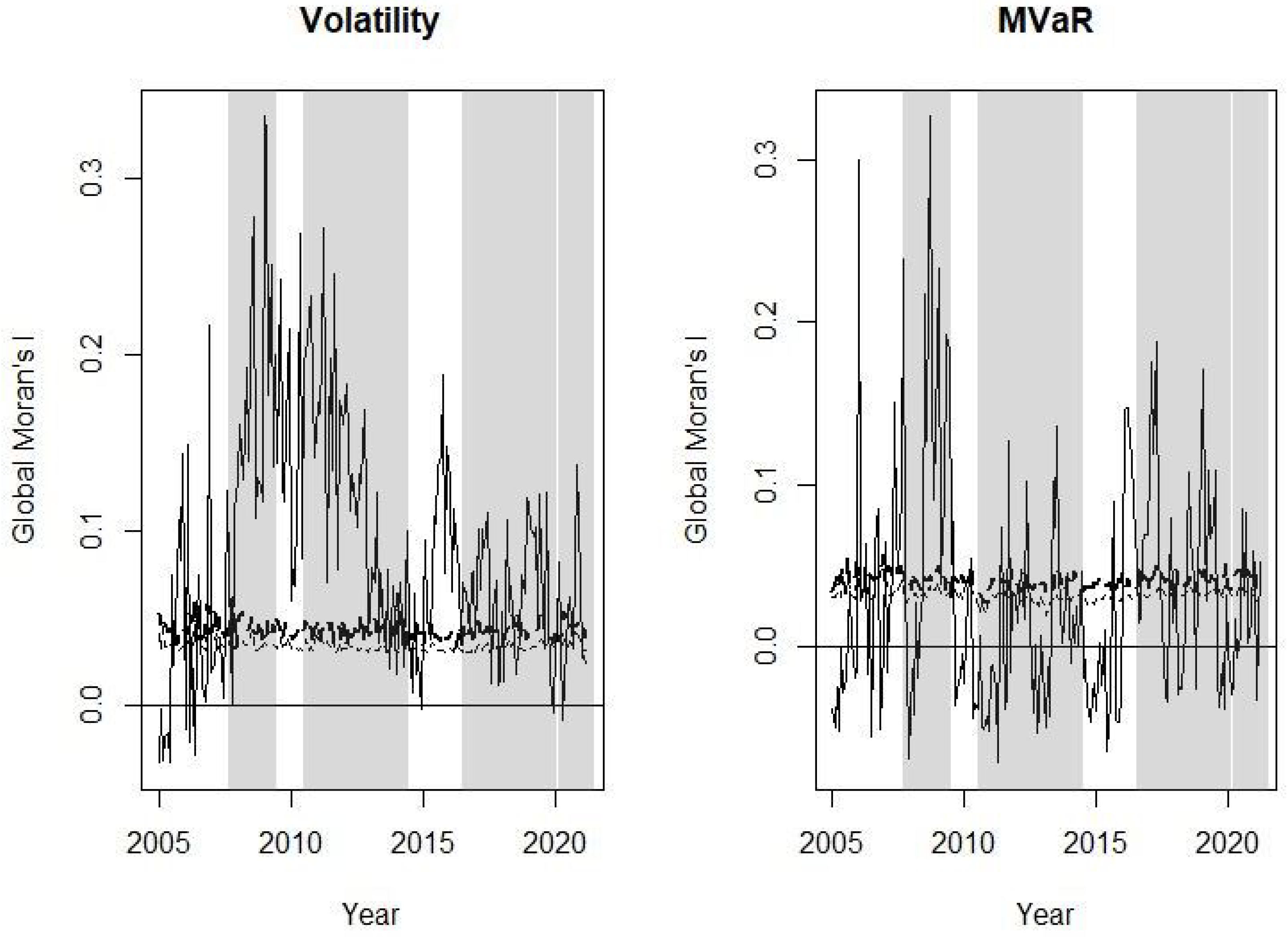
Figure 2 shows that throughout the analysed period the mean of the risk variable is greater than its median, which reflects the skewness of the data due to the presence of extreme risks, especially during the sub-prime period. In the exercise of simulation of Section 3, Table 1 shows that in these cases, when spatial dependence is not significant, normal inference tends to reject the null hypothesis more frequently than bootstrap inference, i.e., the normality assumption increases the error type I. This result is reflected in our analysis in Figure 3 where, along with the value of the global Moran’s I statistic, its upper limits at $95\%$ confidence level are plotted, estimated with normal distribution (thin dashed line) and bootstrap (thick dashed line), with the former always below the latter.

In Figure 3, we observe that positive spatial dependence for volatility is more frequent than for MVaR. This is justified given that the former takes into account both tails of the loss distribution and the latter is focused on the right tail. So, on the right we plot positive spatial dependence between extreme losses. For the volatility, the period with more positive spatial dependence is the sub-prime crisis, followed by the Euro debt crisis; however, for the MVaR, the sub-prime period remains the one that causes the greatest positive spatial dependence between extreme losses but is followed by Brexit. Similar results on the US sub-prime crisis have been obtained in recent work by Chopra and Mehta [25], these authors showed that the sub-prime crisis was the most contagious for the Asian stock markets. In addition, previous works also showed the contagion of this crisis in different financial markets around the world, see [16,17].

To complete the results of Figure 3, in

Table 5. Frequencies and proportion of months with significant positive global spatial dependence and test at $5\%$ significance level of difference between proportion of months with significant positive spatial dependence in each crisis period, with respect to the non-crisis period.

	Volatility			MVaR
Volatility	Frequency	Proportion	p-Value	Frequency	Proportion	p-Value
Sub-prime	22	0.957	0.001	13	0.565	0.010
Euro Debit	42	0.857	0.002	12	0.245	0.287
Brexit	30	0.682	0.239	22	0.500	0.014
COVID-19	6	0.429	0.901	5	0.357	0.316
Total crisis	100	0.769	0.012	52	0.400	0.070
Total no crisis	40	0.615		19	0.292

we show the test of differences of proportions of months with significant positive spatial dependence between each crisis period and the non-crisis period. The results of Table 5 allow us to answer the three questions posed in the Introduction of this study. For volatility, in the four crisis periods the proportion of the months with positive spatial dependence is greater than for the non-crisis period. However, the differences are significant for the sub-prime and Euro debt crises. In contrast, for the spatial dependence estimate with the MVaR, the proportion of months for Euro debt crisis is lower than that for the non-crisis period, although the difference is not significant at the $5\%$ significance level. In this case, the Brexit period reflects a stronger spatial dependence than the Euro debt period. In relation to the COVID-19 pandemic, the results with volatility and MVaR do not show significant differences compared to the non-crisis period. In response to the first question, we can affirm that the volatility spatial dependence, that takes into account the two tails of the distribution (losses and profits), is clearly more frequent in periods of crisis, i.e., spatial dependence occurs in boom and bust periods. Regarding the second and third questions, we observe that there are clear differences between the spatial dependence detected in the different periods of crisis and between spatial dependence criteria (volatility and MVaR).

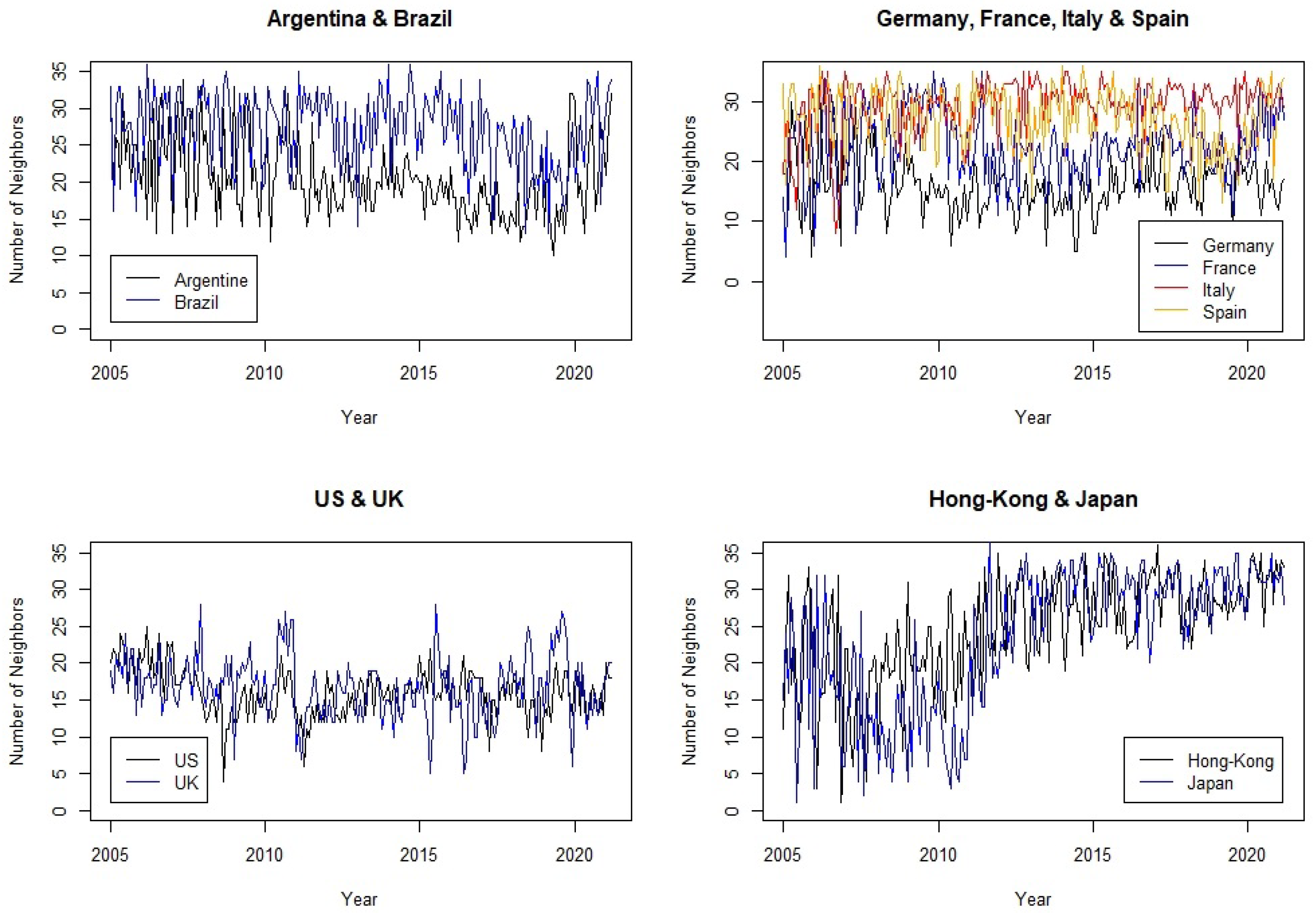
Next, we analyse the local spatial dependency for the market indices of the following countries: Spain, Germany, France, Italy, UK, US, Argentina, Brazil, Japan and Hong Kong, in total 11 indices, given that the US has two. The upper confidence limits are carried out with Bonferroni correction for multiple null hypothesis (11 in our case). In Figure 4, the monthly number of neighbours for different groups of countries is plotted. It is in Japan and Hong Kong where the trend shows an increase. In the EU, Italy has the greatest number of neighbours throughout almost all of the period, followed by Spain, while Germany is the EU country with the fewest neighbours of uncertainty. Argentina is below Brazil and the UK has a more unstable behaviour in terms of number of neighbours than the US.

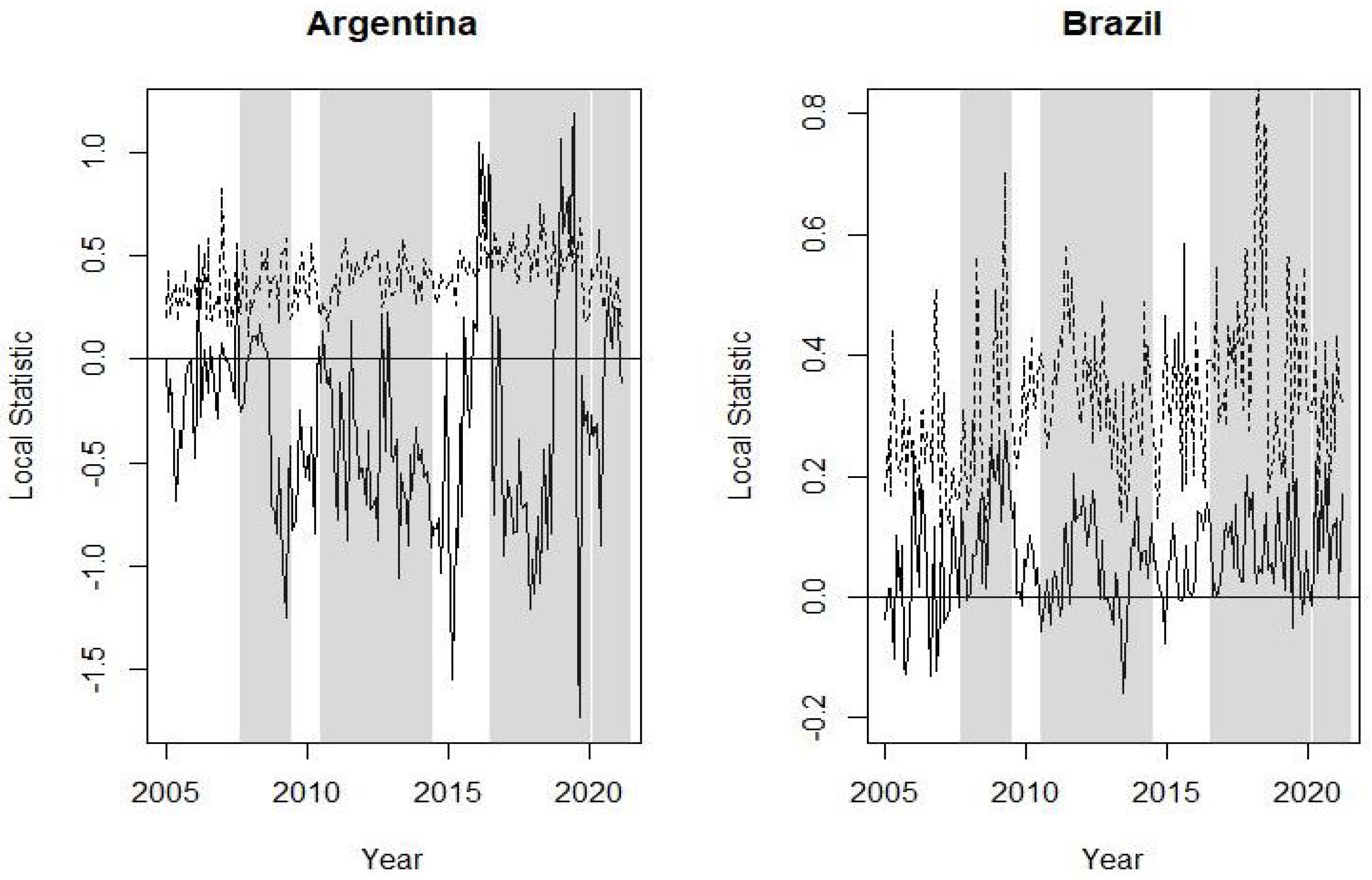
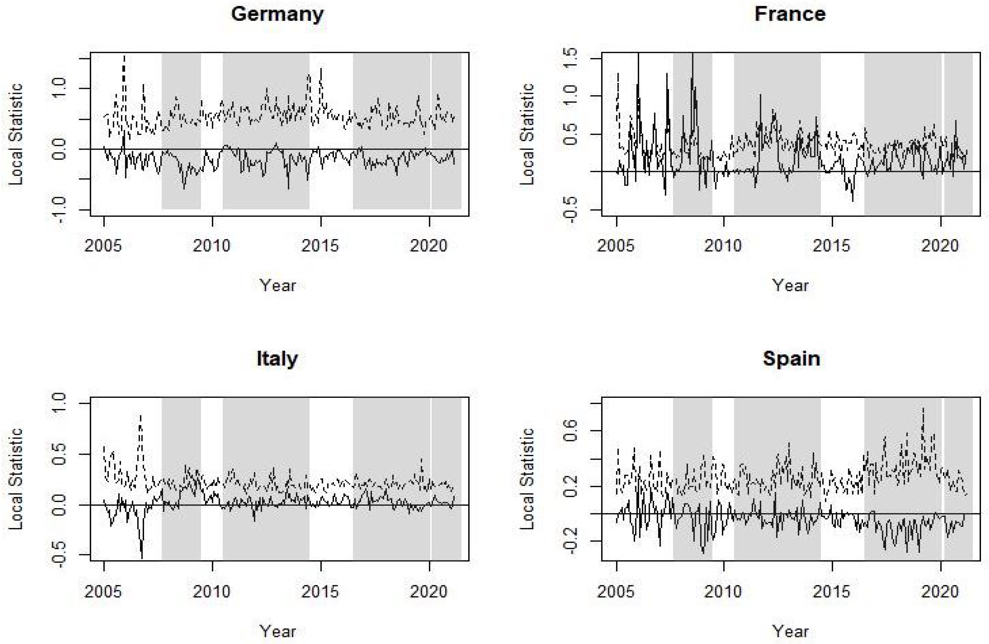
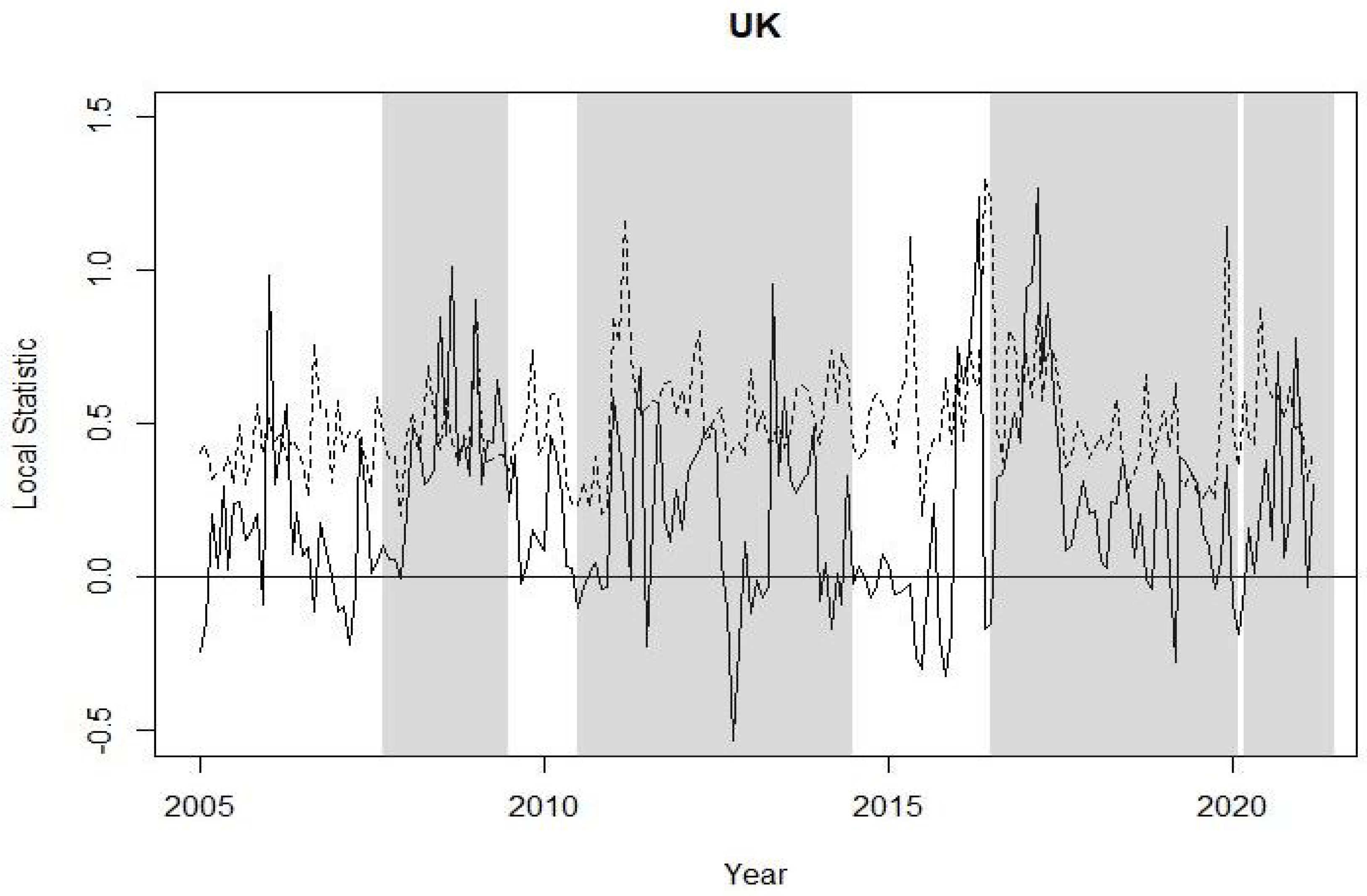
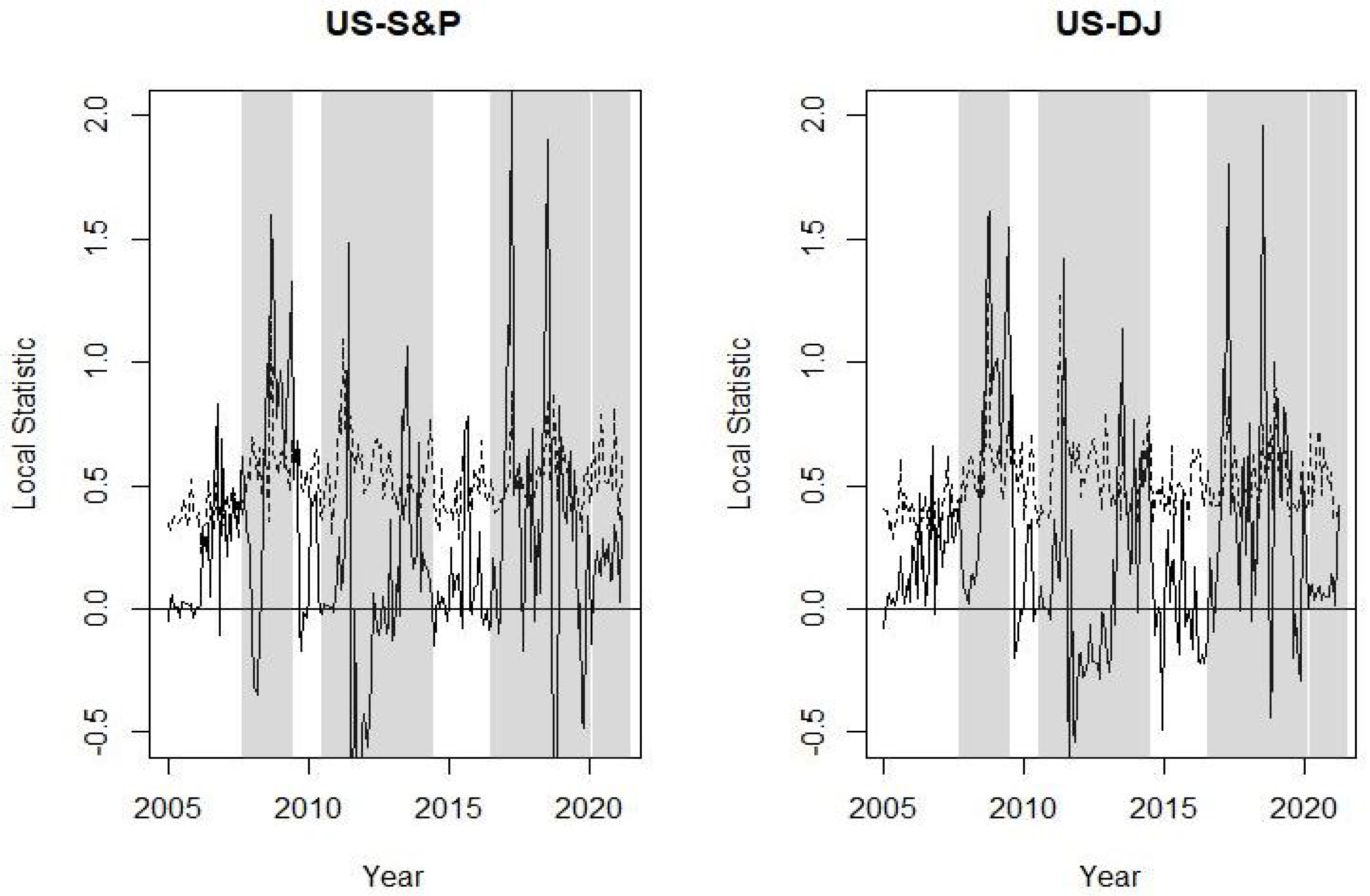
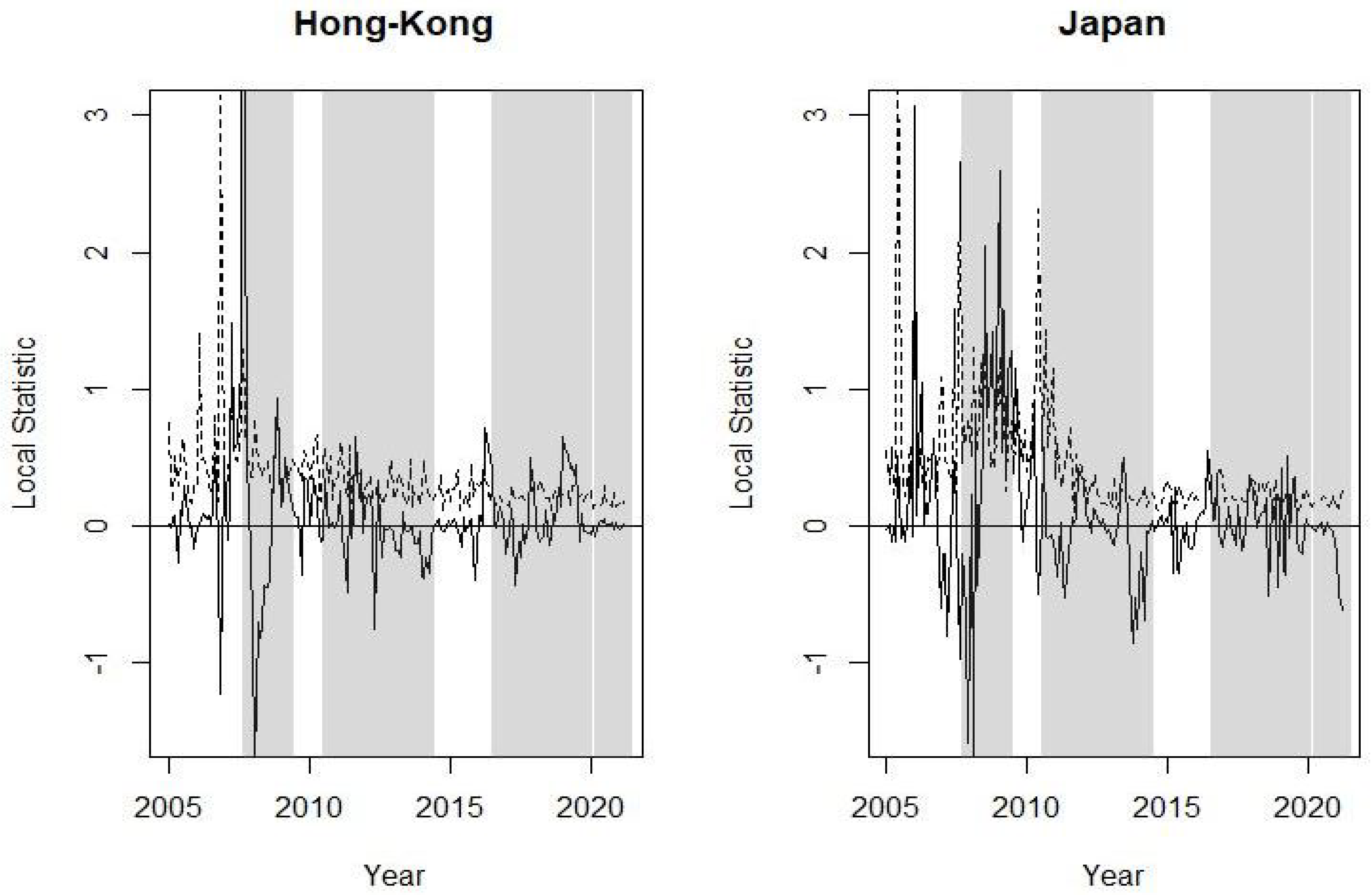
The graphs from Figure 5, Figure 6, Figure 7, Figure 8 and Figure 9 plot the local spatial dependence statistics (solid line) and the bootstrap upper limits at $95\%$ confidence level (dashed line) for testing significant positive local spatial dependence. These figures are obtained focusing on the right tail of the loss distribution, i.e., using MVaR for the 11 indices. Specifically, Figure 5 shows the results for Argentina and Brazil, Figure 6 for the four EU markets, Figure 7 for the UK, Figure 8 for the US and, finally, the local spatial dependence results for Japan and Hong Kong are shown in Figure 9. The results obtained with the volatility are omitted; similar to global spatial dependence, these show a somewhat stronger dependence. A significant local spatial dependence implies that the country spreads its situation of extreme losses to its neighbouring countries, i.e., neighbours with similar uncertainty. These linkages between stock market losses are apparent for some countries and for certain specific periods. Figure 5 shows a significant local positive spatial dependence for Argentina just before the Brexit referendum and at the end of this period. With regard to the EU countries, Figure 6 shows that it is the French stock market that shows a significant spatial dependence before and during the sub-prime period, as well as some months with strong local dependency during the Brexit and COVID-19 period. The UK shows similar results to France, although the period of strong local spatial dependence before and after the Brexit referendum is particularly prominent. The US indices are those that show more frequent local spatial dependence in all the crisis periods apart from during the COVID-19 pandemic. Finally, the two Asian stock markets have significant local spatial dependence in the sub-prime period and more so in Japan.

We observe that between non-EU countries, Argentina has a certain level of contagion both in the sub-prime crisis and due to Brexit, but it is relatively lower compared to the EU countries analysed. It is interesting to note that countries such as Germany and Spain have financial markets relatively isolated from the others, since they do not have relevant spatial correlation.

With respect to the other countries analysed, there are certain relevant impulses: the US indices clearly felt an impact from the Brexit crisis due to their interconnection with the UK economy; France, curiously, has connections for all crises except Brexit, since it has somehow benefited from it.

With regard to the possibility of detecting crises in advance, through relevant impacts on the spatial correlation, we see that the Euro debt crisis does not show any sign of impact, nor does Brexit, but the sub-prime crisis does show in almost all countries an increase in the relevant spatial correlation. We could perhaps consider that the type of crisis can influence contagion before or during it and that the markets adjust their expectations differently depending on what they are like.

5. Conclusions

This article presents a complete study of the analysis of global and local spatial dependence with Moran statistics in the context of financial markets and their uncertainty.

A simulation study is presented which shows how, when there are extreme values in the right tail of the distribution, the inference with global and local Moran statistics based on the normal distribution increases the type I error. The same tests are also done based on the bootstrap resampling technique.

Following the analysis of the data, there are some interesting findings. The period of the global financial crisis of the sub-prime is the one that caused more linkages between the extreme losses of the analysed stock indices. We can therefore conclude that systemic risk in this period caused more losses than in the others periods. The Euro debt period is the one with less global spatial dependence between extreme losses, followed by the COVID-19 pandemic period. Between the 10 countries whose local spatial dependences were analysed, those that were contagious for their neighbours of uncertainty in certain months were Argentina, France, the US, the UK, Japan and Hong Kong.

The impact of the financial crisis of the sub-prime is the most visible in our study such that it presents a greater presence of joint or systemic risk, where the most extreme losses are greater. However, the opposite is seen in two other crises analysed, Euro debt and COVID-19. We consider that a possible justification for this comes from the fact that their impact was more indirect on the markets and more adequate management tools were created. With regard to Brexit, which was consolidated little by little, we see that there are no signs of contagion before it, but there are during it in the countries with more interconnected economies: the US, Hong Kong, Japan and, of course, the UK. Finally, we would like to mention a degree of isolation of certain countries in terms of contagion—Germany, Spain, Italy and Brazil—this may because these countries have different structures than those that are more closely related. The greater variability of the Local Moran indicator itself could be an early indicator of the crises themselves, and detecting which markets are more sensitive to them could be a way of preparing the latter for any adjustments needed.

References

- McNeil, A.J.; Frey, R.; Embrechts, P. Quantitative Risk Management: Concepts, Techniques and Tools; Revised ed.; Princeton University Press: Princeton, NJ, USA, 2015. [Google Scholar]
- Moran, P.A.P. Notes on continuous stochastic phenomena. Biometrika 1950, 37, 17–23. [Google Scholar] [CrossRef] [PubMed]
- Anselin, L. Local indicators of spatial association - LISA. Geogr. Anal. 1995, 27, 93–115. [Google Scholar] [CrossRef]
- Griffith, D.A. The Moran coefficient for non-normal data. J. Stat. Plan. Inference 2010, 140, 2980–2990. [Google Scholar] [CrossRef]
- Yang, Z. LM tests of spatial dependence based on bootstrap critical values. J. Econ. 2015, 185, 33–59. [Google Scholar] [CrossRef]
- Jin, F.; Lee, L.F. On the bootstrap for Moran’I test for spatial dependence. J. Econ. 2015, 184, 295–314. [Google Scholar] [CrossRef]
- Mei, C.L.; Xu, S.F.; Chen, F. Consistency of bootstrap approximation to the null distributions of local spatial statistics with application to house price analysis. J. Inequal. Appl. 2020, 217, 2–19. [Google Scholar] [CrossRef]
- Acuña, C.A.; Bolancé, C.; Torra, S. Análisis de la dependencia espacial entre índices bursátiles. Anal. Inst. Act. Españoles 2018, 24, 79–97. [Google Scholar]
- Flavin, T.; Hurley, M.J.; Rousseau, F. Explaining Stock Market Correlation: A Gravity Model Approach. Manch. Sch. 2002, 70, 87–106. [Google Scholar] [CrossRef] [Green Version]
- Ahir, H.; Bloom, N.; Furceri, D. The World Uncertainty Index; Technical Report 19–027, SIEPR-Stanford Institute for Economic Policy Research; National Bureau of Economic Research-Stanford (US): Stanford, CA, USA, 2019. [Google Scholar]
- Baker, S.R.; Bloom, N.; Davis, S.J. Measuring Economic Policy Uncertainty. Quar. J. Econ. 2016, 131, 1593–1636. [Google Scholar] [CrossRef]
- Ghirelli, C.; Pérez, J.J.; Urtasun, A. A new economic policy uncertainty index for Spain. Econ. Lett. 2019, 182, 64–67. [Google Scholar] [CrossRef] [Green Version]
- Weinberg, L. The Google Trends Uncertainty (GTU) Index: A Measure of Economic Policy Uncertainty in the EU Using Google Trends. Undergr. Econ. Rev. 2020, 17, 2. [Google Scholar]
- Castelnuovo, E.; Tran, T.D. Google It Up! A Google Trends-based Uncertainty Index for the United States and Australia. Econ. Lett. 2017, 161, 149–153. [Google Scholar] [CrossRef] [Green Version]
- Dimitriou, D.; Kenourgios, D.; Simos, T. Global financial crisis and emerging stock market contagion: A multivariate FIAPARCH-DCC approach. Int. Rev. Financ. Anal. 2013, 30, 46–56. [Google Scholar] [CrossRef]
- Lien, D.; Lee, G.; Yang, L.; Zhang, Y. Volatility spillovers among the US and Asian stock markets: A comparison between the periods of Asian currency crisis and subprime credit crisis. N. Am. J. Econ. Financ. 2018, 46, 187–201. [Google Scholar] [CrossRef]
- Mohti, W.; Dionísio, A.; Ferreira, P.; Vieira, I. Contagion of the Subprime Financial Crisis on Frontier Stock Markets: A Copula Analysis. Economies 2019, 7, 15. [Google Scholar] [CrossRef] [Green Version]
- Tilfani, O.; Ferreira, P.; Boukfaoui, M.Y.E. Dynamic cross-correlation and dynamic contagion of stock markets: A sliding windows approach with the DCCA correlation coefficient. Empirical Econ. 2021, 60, 1127–1156. [Google Scholar] [CrossRef]
- Samarakoon, L.P. Contagion of the Eurozone debt crisis. J. Int. Financ. Mark. Inst. Mon. 2017, 49, 115–128. [Google Scholar] [CrossRef]
- Samitas, A.; Tsakalos, I. How can a small country affect the European economy? The Greek contagion phenomenon. J. Int. Financ. Mark. Inst. Mon. 2013, 25, 18–32. [Google Scholar] [CrossRef]
- Breinlich, H.; Leromain, E.; Novy, D.; Sampson, T.; Usman, A. The Economic Effects of Brexit: Evidence from the Stock Market. Fiscal Stud. 2018, 39, 581–623. [Google Scholar] [CrossRef]
- Ameur, H.B.; Louhichi, W. The Brexit impact on European market co-movements. Ann. Oper. Res. 2021. Available online: https://0-link-springer-com.brum.beds.ac.uk/article/10.1007/s10479-020-03899-9 (accessed on 25 February 2022).
- Li, H. Volatility spillovers across European stock markets under the uncertainty of Brexit. Econ. Model. 2020, 84, 1–12. [Google Scholar] [CrossRef]
- Burdekin, R.C.K.; Hughson, E.; Gu, J. A first look at Brexit and global equity markets. Appl. Econ. Lett. 2018, 25, 136–140. [Google Scholar] [CrossRef]
- Chopra, M.; Mehta, C. Is the COVID-19 pandemic more contagious for the Asian stock markets? A comparison with the Asian financial, the US subprime and the Eurozone debt crisis. J. Asian Econ. 2022, 79, 101450. [Google Scholar] [CrossRef] [PubMed]
- Li, Y.; Liang, C.; Ma, F.; Wang, J. The role of the IDEMV in predicting European stock market volatility during the COVID-19 pandemic. Financ. Res. Lett. 2020, 36, 101749. [Google Scholar] [CrossRef] [PubMed]
- Baker, S.R.; Bloom, N.; Davis, S.J.; Kost, K.; Sammon, M.; Viratyosin, T. The Unprecedented Stock Market Reaction to COVID-19. Rev. Asset Pricing Stud. 2020, 10, 742–758. [Google Scholar] [CrossRef]
- Akhtaruzzaman, M.; Boubaker, S.; Sensoy, A. Financial contagion during COVID-19 crisis. Financ. Res. Lett. 2021, 38, 101604. [Google Scholar] [CrossRef]
- Asgharian, H.; Hess, W.; Liu, L. A spatial analysis of international stock market linkages. J. Banking Financ. 2013, 37, 4738–4754. [Google Scholar] [CrossRef]
Figure 1.
Losses (left) and standardised residuals of filtered losses (right) for the 46 stock indices.
Figure 2.
Volatility (left) and MVaR at 99% confidence level (right). The crisis periods are shaded. Mean values plotted in magenta long dashed line and median in yellow short dashed line.
Figure 3.
Global Moran’s I statistic for Volatility (left) and for MVaR at confidence level (right). The crisis periods are shaded. Upper limits at confidence level that have been estimated with normal distribution (thin dashed line) and bootstrap (thick dashed line).
Figure 4.
Number of neighbours.
Figure 5.
Local Moran statistic for MVaR at confidence level (solid line) and bootstrap upper limits at confidence level (dashed line). The crisis periods are shaded. Results for Argentine and Brazil stock indices.
Figure 6.
Local Moran statistic for MVaR at confidence level (solid line) and bootstrap upper limits at confidence level (dashed line). The crisis periods are shaded. Results for EU stock indices.
Figure 7.
Local Moran statistic for MVaR at confidence level (solid line) and bootstrap upper limits at confidence level (dashed line). The crisis periods are shaded. Results for UK stock index.
Figure 8.
Local Moran statistic for MVaR at confidence level (solid line) and bootstrap upper limits at confidence level (dashed line). The crisis periods are shaded. Results for US stock indices.
Figure 9.
Local Moran statistic for MVaR at confidence level (solid line) and bootstrap upper limits at confidence level (dashed line). The crisis periods are shaded. Results for Japan and Hong Kong stock indices.