Article

Global Properties of a Diffusive SARS-CoV-2 Infection Model with Antibody and Cytotoxic T-Lymphocyte Immune Responses

1
Department of Mathematics, Faculty of Science, King Abdulaziz University, P.O. Box 80203, Jeddah 21589, Saudi Arabia
2
Department of Mathematics, Faculty of Science, Al-Azhar University, Assiut Branch, Assiut 71516, Egypt
*
Author to whom correspondence should be addressed.
Submission received: 8 December 2022 / Revised: 22 December 2022 / Accepted: 25 December 2022 / Published: 29 December 2022

Abstract

:
A severe acute respiratory syndrome coronavirus 2 (SARS-CoV-2) infection can lead to morbidity and mortality. SARS-CoV-2 infects the epithelial cells of the respiratory tract and causes coronavirus disease 2019 (COVID-19). The immune system’s response plays a significant role in viral progression. This article develops and analyzes a system of partial differential equations (PDEs), which describe the in-host dynamics of SARS-CoV-2 under the effect of cytotoxic T-lymphocyte (CTL) and antibody immune responses. The model characterizes the interplay between six compartments, healthy epithelial cells (ECs), latent infected ECs, active infected ECs, free SARS-CoV-2 particles, CTLs, and antibodies. We consider the logistic growth of healthy ECs. We first investigate the properties of the model’s solutions, then, we calculate all steady states and determine the conditions of their existence and global stability. The global asymptotic stability is examined by constructing Lyapunov functions. The analytical findings are supported via numerical simulations.

1. Introduction

Recently, many viruses have spread that infect the human body, which can lead to illness and death and thus have a great impact on health and the global economy. These viruses include human viral infections such as human T-cell lymphotropic virus (HTLV), human immunodeficiency virus (HIV), Ebola virus, hepatitis B virus, hepatitis C virus, influenza virus, chikungunya virus, Middle East Respiratory Syndrome coronavirus (MERS-CoV), Zika virus, and dengue virus. At the end of 2019, the world witnessed the emergence of a new respiratory virus in Wuhan, China, called severe acute respiratory syndrome coronavirus 2 (SARS-CoV-2), which causes coronavirus disease 2019 (COVID-19). Within a few months, this viral infection had spread to most countries in the world and infected many people of different ages. Since the beginning of the spread of the virus, scientists from many disciplines have focused on finding ways to confront this pandemic such as by applying suitable control methods to reduce viral transmission, synthesizing antiviral drugs, and synthesizing vaccinations [1,2]. The WHO approved eleven vaccines for COVID-19 for emergency use [3]. Disease progression and outcome in COVID-19 are highly dependent on the host immune response, particularly in the elderly in whom immunosenescence may predispose them to increased risk of infection [4]. Immunosenescence enhances the susceptibility to viral infections and renders vaccinations less effective [5].
SARS-CoV-2 is a single-stranded positive-sense RNA virus and is a member of the Coronaviridae family. It is an airborne-transmitted virus and can infect the upper and lower respiratory tracts [6]. The epithelial cells (ECs) of the host respiratory tract are the target for SARS-CoV-2 particles [7]. The in-host dynamics of SARS-CoV-2 were mathematically modeled in [8] as
d E ( t ) d t = ψ E ( t ) S ( t ) SARS-CoV- 2 infectious transmission , d W ( t ) d t = ψ E ( t ) S ( t ) SARS-CoV- 2 infectious transmission ϑ W ( t ) latent transition , d P ( t ) d t = ϑ W ( t ) latent transition β P P ( t ) natural death , d S ( t ) d t = ϱ P ( t ) SARS-CoV- 2 production β S S ( t ) natural death ,
where E, W, P, and S represent the concentrations of healthy ECs, latent infected ECs, active infected ECs, and SARS-CoV-2 particles, respectively. Li et al. [9] considered the regeneration and death of uninfected ECs
d E ( t ) d t = β E ( E ( 0 ) E ( t ) ) ψ E ( t ) S ( t ) ,
where E ( 0 ) is the initial concentration of healthy ECs.
Several extensions and modifications have been made on the SARS-CoV-2 infection models presented in [8,9] by taking into consideration the effect of different drug therapies [10,11,12] and the influence of time delay [13]. The innate immune response represents the first line of defense that recognizes the antigens and activates the adaptive immune response. B cells and T cells are important components of the adaptive immune response. It has been reported in [14] that both B- and T-cell responses against SARS-CoV-2 are detected in the blood around 1 week after the onset of COVID-19 symptoms. B cells have the ability to produce antibodies specific to SARS-CoV-2, such as IgA, IgG, and IgM, in order to neutralize the virus at the infection site [15,16,17,18]. CD8 + T cells (also known as cytotoxic T lymphocytes (CTLs)) are important for directly attacking and killing SARS-CoV-2-infected epithelial cells, whereas CD4 + T cells are crucial to prime both B cells and CTLs. CD4 + T cells are also responsible for cytokine production to drive immune cell recruitment [14]. The impact of the immune response was introduced in the SARS-CoV-2 infection model in [19,20,21,22,23,24,25]. Elaiw et al. [13] added a logistic term for the proliferation of healthy ECs as
d E ( t ) d t = ϕ β E E ( t ) + υ E ( t ) 1 E ( t ) E m a x ψ E ( t ) S ( t ) .
It was assumed that healthy ECs are regenerated with a constant ϕ and are proliferated with a logistic growth rate υ E 1 E E m a x , where υ is the rate of growth and E m a x is the maximum capacity of healthy ECs in the human body.
Stability analysis for models describing the in-host dynamics of SARS-CoV-2 infection was conducted in [23,24,25,26,27,28]. Hattaf and Yousfi [23] studied the global stability of an in-host SARS-CoV-2 infection model with cell-to-cell transmission and the cytotoxic T-lymphocyte (CTL) immune response. The model included both lytic (destruction of infected cells [29]) and nonlytic (inhibition of viral replication by soluble mediators secreted by immune cells [29]) immune responses. A SARS-CoV-2 infection model with both CTL and antibody immunities was developed and analyzed in [24]. Mathematical analysis of the model presented in [9] was studied in [26]. Both local and global stability analyses of the model’s equilibria were established. Almocera et al. [25] studied the stability of the two-dimensional SARS-CoV-2 dynamics model with the immune response presented in [8]. Elaiw et al. [13] studied the global stability of a delayed SARS-CoV-2 dynamics model with the logistic growth of uninfected ECs and antibody immunity. In very recent works, the Lyapunov method was used to establish the global stability of co-infection models including SARS-CoV-2/HIV-1 [27], SARS-CoV-2/Influenza A virus [28], and SARS-CoV-2/malaria [30].
In all the above mentioned works, it was assumed that the viruses and cells are homogeneously distributed in the human body. However, such an assumption is unrealistic because the diffusion of viruses and cells causes spatial variations within the body. Spatial structure plays a major role in describing the dynamical behaviors of SARS-CoV-2 infection within a host. The effect of spatial structure on the SARS-CoV-2 dynamics was addressed in [31,32]. In these papers, it was assumed that SARS-CoV-2 infection is resisted by antibodies, whereas the effect of CTL immunity was neglected. Moreover, the proliferation of healthy ECs was not included. In the present article, we construct and analyze a diffusive SARS-CoV-2 infection model with both antibody and CTL immune responses. We prove the non-negativity and boundedness of the solutions. We consider the logistic growth of healthy ECs. We derive the threshold parameters that determine the existence and stability of the model’s steady states. The global stability of all steady states is established by constructing Lyapunov functions and applying LaSalle’s invariance principle (LIP). We illustrate our theoretical results with some numerical simulations.

2. Model Formulation

We propose a diffusive SARS-CoV-2 model with antibody and CTL immune responses. Let E ( x , t ) , W ( x , t ) , P ( x , t ) , S ( x , t ) , H ( x , t ) , and M ( x , t ) be the concentrations of healthy ECs, latent infected cells, active infected ECs, SARS-CoV-2 particles, antibodies, and CTLs, respectively, at spatial location x and time t.
E ( x , t ) t = D E Δ E ( x , t ) + ϕ β E E ( x , t ) + υ E ( x , t ) 1 E ( x , t ) E m a x ψ E ( x , t ) S ( x , t ) ,
W ( x , t ) t = D W Δ W ( x , t ) + γ ψ S ( x , t ) E ( x , t ) ϑ W ( x , t ) β W W ( x , t ) ,
P ( x , t ) t = D P Δ P ( x , t ) + ( 1 γ ) ψ S ( x , t ) E ( x , t ) + ϑ W ( x , t ) β P P ( x , t ) σ P ( x , t ) M ( x , t ) ,
S ( x , t ) t = D S Δ S ( x , t ) + ϱ P ( x , t ) β S S ( x , t ) λ S ( x , t ) H ( x , t ) ,
H ( x , t ) t = D H Δ H ( x , t ) + μ S ( x , t ) H ( x , t ) β H H ( x , t ) ,
M ( x , t ) t = D M Δ M ( x , t ) + η P ( x , t ) M ( x , t ) β M M ( x , t ) ,
where x = x 1 , x 2 , , x m ϖ and t > 0 . The spatial domain ϖ R m , m 1 is connected and bounded and the boundary ϖ is smooth. Δ = 2 x 2 is the Laplacian operator and D Q is the diffusion coefficient of Q { E , W , P , S , H , M } . Parameter γ ( 0 , 1 ) is the part of the healthy ECs that enters the latent state and β W W is the death rate of the latent infected ECs. The active infected ECs are killed by CTLs at rate σ M P . The SARS-CoV-2 particles are neutralized by antibodies at the rate λ H S . The terms μ H S and η M P represent the proliferation rates of antibodies and CTLs, respectively. The terms β H H and β M M denote the death rate of antibodies and CTLs, respectively. The initial conditions are given by
E ( x , 0 ) = δ 1 ( x ) , W ( x , 0 ) = δ 2 ( x ) , P ( x , 0 ) = δ 3 ( x ) , S ( x , 0 ) = δ 4 ( x ) , H ( x , 0 ) = δ 5 ( x ) , M ( x , 0 ) = δ 6 ( x ) , x ϖ ¯ ,
where δ i ( x ) , i = 1 , , 6 , are non-negative and continuous functions. In addition, we consider the following homogeneous Neumann boundary conditions:
E n = W n = P n = S n = H n = M n = 0 , t > 0 , x ϖ ,
where n is the outward normal derivative on the boundary ϖ .

3. Properties of Solutions

This section examines the existence, non-negativity, and boundedness of the solutions of Systems (2)–(7) with the initial conditions in (8) and the boundary conditions in (9). Moreover, it determines the existence conditions of the spatially homogeneous steady states of the model.
Theorem 1.
Assume that D E = D W = D P = D S = D H = D M = D . Then, Models (2)–(7) have unique, non-negative, and bounded solutions defined on ϖ ¯ × [ 0 , + ) for any given initial data satisfying (8).
Proof. 
Let X = B U M ϖ ¯ , R 6 be the set of all bounded and uniformly continuous functions from ϖ ¯ to R 6 , and X + = B U M ϖ ¯ , R + 6 X . Hence, the positive cone X + induces a partial order on X . Define θ X = sup x ϖ ¯ | θ ( x ) | , where | · | is the Euclidean norm on R 6 . It follows that the space X , · X is a Banach lattice [33,34]. □
For any initial data δ = ( δ 1 , δ 2 , δ 3 , δ 4 , δ 5 , δ 6 ) X + , we define Γ = ( Γ 1 , Γ 2 , Γ 3 , Γ 4 , Γ 5 , Γ 6 ) : X + X by
Γ 1 ( δ ) ( x ) = ϕ β E δ 1 ( x ) + υ δ 1 ( x ) 1 δ 1 ( x ) E m a x ψ δ 1 ( x ) δ 4 ( x ) , Γ 2 ( δ ) ( x ) = γ ψ δ 1 ( x ) δ 4 ( x ) ϑ δ 2 ( x ) β W δ 2 ( x ) , Γ 3 ( δ ) ( x ) = ( 1 γ ) ψ δ 1 ( x ) δ 4 ( x ) + ϑ δ 2 ( x ) β P δ 3 ( x ) σ δ 3 ( x ) δ 6 ( x ) , Γ 4 ( δ ) ( x ) = ϱ δ 3 ( x ) β S δ 4 ( x ) λ δ 4 ( x ) δ 5 ( x ) , Γ 5 ( δ ) ( x ) = μ δ 4 ( x ) δ 5 ( x ) β H δ 5 ( x ) , Γ 6 ( δ ) ( x ) = η δ 3 ( x ) δ 6 ( x ) β M δ 6 ( x ) .
We observe that Γ is locally Lipschitz on X + . Models (2)–(7) with Conditions (8) and (9) can be written as the following abstract functional DE
d Q d t = D Q + Γ ( Q ) , t > 0 , Q ( 0 ) = δ X + ,
where Q = ( E , W , P , S , H , M ) and D Q = D E Δ E , D W Δ W , D P Δ P , D S Δ S , D H Δ H , D M Δ M . can be shown that
lim h 0 + 1 h dist δ ( 0 ) + h Γ ( δ ) , X + = 0 , for all δ X + .
It follows from [33,34,35] that for any δ X + , Systems (2)–(7) with (8) and (9) have unique non-negative mild solutions ( E x , t , W x , t , P x , t , S x , t , H x , t , M x , t ) defined on ϖ ¯ × [ 0 , T max ) , where [ 0 , T max ) is the maximal existence time interval on which the solution exists. Further, this solution is also a classical solution for the given problem.
Now, we define
Φ x , t = E x , t + W x , t + P x , t + β P 2 ϱ S x , t + β P λ 2 ϱ μ H x , t + σ η M x , t .
Since D E = D W = D P = D S = D H = D M = D , then, using Systems (2)–(7) we obtain
Φ ( x , t ) t D Δ Φ ( x , t ) = ϕ β E E ( x , t ) + υ E ( x , t ) 1 E ( x , t ) E m a x β W W ( x , t ) β P 2 P ( x , t ) β P β S 2 ϱ S ( x , t ) β P β H λ 2 ϱ μ H ( x , t ) β M σ η M ( x , t ) = υ E m a x E 2 ( x , t ) + υ E ( x , t ) + ϕ β E E ( x , t ) β W W ( x , t ) β P 2 P ( x , t ) β P β S 2 ϱ S ( x , t ) β P β H λ 2 ϱ μ H ( x , t ) β M σ η M ( x , t ) .
Let us define Π ( E ) = υ E m a x E 2 + υ E + ϕ and calculate Π ( E ) as
Π ( E ) = 2 υ E m a x E + υ = 0 E = E m a x 2
and
Π ( E ) = 2 υ E m a x < 0 .
Then,
Π E m a x 2 = υ E m a x E m a x 2 2 + υ E m a x 2 + ϕ = υ E m a x 4 + ϕ .
Let N 1 = υ E m a x + 4 ϕ 4 > 0 and q 1 = min { β E , β W , β P 2 , β S , β H , β M } , then, Φ ( x , t ) satisfies the following system:
Φ ( x , t ) t D Δ Φ ( x , t ) N 1 q 1 Φ ( x , t ) , Φ n = 0 , Φ ( x , 0 ) = δ 1 ( x ) + δ 2 ( x ) + δ 3 ( x ) + β P 2 ϱ δ 4 ( x ) + β P λ 2 ϱ μ δ 5 ( x ) + σ η δ 6 ( x ) 0 .
Let Φ ˜ ( t ) be a solution to the following ODE system
d Φ ˜ ( t ) d t = N 1 q 1 Φ ˜ ( t ) , Φ ˜ ( 0 ) = max x ϖ ¯ Φ ( x , 0 ) .
This gives that Φ ˜ ( t ) max N 1 q 1 , max x ϖ ¯ Φ ( x , 0 ) . According to the comparison principle [36], we have Φ ( x , t ) Φ ˜ ( t ) . Then, we obtain
Φ ( x , t ) max N 1 q 1 , max x ϖ ¯ Φ ( x , 0 ) ,
which implies that E x , t , W x , t , P x , t , S x , t , H x , t , and M x , t are bounded on ϖ ¯ × [ 0 , T max ) . From the standard theory for semi-linear parabolic systems, we deduce that T max = + [37]. This shows that solution E x , t , W x , t , P x , t , S x , t , H x , t , M x , t is defined for all x ϖ , t > 0 and is also non-negative and unique.

4. Steady States

This section computes all steady states of Systems (2)–(7) and the threshold parameters that guarantee the existence of these steady states. Let S S = ( E , W , P , S , H , M ) be any steady state of Systems (2)–(7) satisfying the following system of nonlinear equations:
0 = ϕ β E E + υ E 1 E E m a x ψ E S ,
0 = γ ψ E S ( ϑ + β W ) W ,
0 = ( 1 γ ) ψ E S + ϑ W β P P σ M P ,
0 = ϱ P β S S λ H S ,
0 = μ H S β H H ,
0 = η M P β M M .
By solving Systems (10)–(15), we find that Systems (2)–(7) have the following steady states:
(i) Healthy steady state S S 0 = ( E 0 , 0 , 0 , 0 , 0 , 0 ) , where E 0 is the positive root of ϕ β E E + υ E 1 E E m a x = 0 and is given by
E 0 = E m a x 2 υ υ β E + ( υ β E ) 2 + 4 υ ϕ E m a x .
The basic reproduction number R 0 for Systems (2)–(7) is given by
R 0 = ϱ ψ E 0 β P β S ρ .
where, ρ = ϑ γ ϑ + β W + 1 γ .
(ii) Infected steady state with inactive immune responses S S 1 = ( E 1 , W 1 , P 1 , S 1 , 0 , 0 ) , where
E 1 = β P β S ϱ ψ ρ = E 0 R 0 , W 1 = γ ϑ + β W ψ E 1 S 1 , P 1 = β S ϱ S 1 , S 1 = ϕ ϱ ρ β P β S + υ ψ β E ψ + υ β P β S ϱ ψ 2 E m a x ρ .
Assume that β E υ + υ E 1 E m a x > 0 , then, we obtain
β E υ + υ E m a x β P β S ϱ ψ ρ > 0 .
We note that
R 0 > 1 E m a x 2 υ υ β E + ( υ β E ) 2 + 4 υ ϕ E m a x > β P β S ϱ ψ ρ ( υ β E ) 2 + 4 υ ϕ E m a x > 2 υ β P β S ϱ ψ E m a x ρ ( υ β E ) .
From Inequality (17), we have 2 υ β P β S ϱ ψ E m a x ρ ( υ β E ) > 0 . Then,
R 0 > 1 4 υ ϕ E m a x > 4 υ 2 β P β S ϱ 2 ψ 2 E m a x 2 ρ 2 4 υ β P β S ϱ ψ E m a x ρ ( υ β E ) υ ϕ > υ 2 β P β S ϱ 2 ψ 2 E m a x ρ 2 υ 2 β P β S ϱ ψ ρ + υ β E β P β S ϱ ψ ρ ϕ ϱ ρ β P β S + υ ψ β E ψ + υ β P β S ϱ ψ 2 E m a x ρ > 0 S 1 > 0 .
Thus, S S 1 exists when R 0 > 1 and β E υ + υ E 1 E m a x > 0 . At this steady state, the virus exists while the immune response is inhibited.
(iii) Infected steady state with only active antibody immunity S S 2 = ( E 2 , W 2 , P 2 , S 2 , H 2 , 0 ) , where
E 2 = E m a x 2 υ υ β E β H ψ μ + υ β E β H ψ μ 2 + 4 υ ϕ E m a x , W 2 = β H γ ψ μ ( ϑ + β W ) E m a x 2 υ υ β E β H ψ μ + υ β E β H ψ μ 2 + 4 υ ϕ E m a x = β H γ ψ E 2 μ ( ϑ + β W ) , P 2 = β H ψ μ β P E m a x 2 υ υ β E β H ψ μ + υ β E β H ψ μ 2 + 4 υ ϕ E m a x ρ = β H ψ E 2 μ β P ρ , S 2 = β H μ , H 2 = β S λ ϱ ψ β P β S E m a x 2 υ υ β E β H ψ μ + υ β E β H ψ μ 2 + 4 υ ϕ E m a x ρ 1 = β S λ ϱ ψ E 2 β P β S ρ 1 .
We note that S S 2 exists when ϱ ψ E 2 β P β S ρ > 1 . Let R 1 H be the antibody immunity activation number defined as
R 1 H = ϱ ψ E 2 β P β S ρ .
which determines when the antibody immunity is activated. Thus, H 2 = β S λ R 1 H 1 . We note that H 2 > 0 when R 1 H > 1 . Thus, S S 2 exists when R 1 H > 1 .
(iv) Infected steady state with only active CTL immunity S S 3 = ( E 3 , W 3 , P 3 , S 3 , 0 , M 3 ) , where
E 3 = E m a x 2 υ υ β E β M ϱ ψ β S η + υ β E β M ϱ ψ β S η 2 + 4 υ ϕ E m a x , W 3 = β M γ ϱ ψ β S η ( ϑ + β W ) E m a x 2 υ υ β E β M ϱ ψ β S η + υ β E β M ϱ ψ β S η 2 + 4 υ ϕ E m a x = β M γ ϱ η ψ E 3 β S η ( ϑ + β W ) , P 3 = β M η , S 3 = β M ϱ β S η , M 3 = β P σ ϱ ψ E 3 β P β S ϑ γ ϑ + β W + 1 γ 1 = β P σ ϱ ψ E 3 β P β S ρ 1 .
We note that M 3 > 0 when ϱ ψ E 3 β P β S ρ > 1 . Then, we define the CTL immunity activation number R 1 M as
R 1 M = ϱ ψ E 3 β P β S ρ .
Consequently, S S 3 exists when R 1 M > 1 .
(v) Infected steady state with both active antibody and CTL immunities S S 4 = ( E 4 , W 4 , P 4 , S 4 , H 4 , M 4 ) , where
E 4 = E m a x 2 υ υ β E β H ψ μ + υ β E β H ψ μ 2 + 4 υ ϕ E m a x = E 2 , W 4 = β H γ ψ μ ( ϑ + β W ) E m a x 2 υ υ β E β H ψ μ + υ β E β H ψ μ 2 + 4 υ ϕ E m a x = β H γ ψ E 4 μ ( ϑ + β W ) , P 4 = β M η = P 3 , S 4 = β H μ = S 2 , H 4 = β M ϱ μ β H η λ β S λ = β S λ β M ϱ μ β S β H η 1 , M 4 = η β M σ β H ψ E 4 μ ϑ γ ϑ + β W + 1 γ β P β M η = β P σ β H η ψ E 4 β P β M μ ρ 1 .
We see that, H 4 and M 4 exist when β M ϱ μ β S β H η > 1 and β H η ψ E 4 β P β M μ ρ > 1 . Now, we define
R 2 M = β H η ψ E 4 β P β M μ ρ .
Hence, H 4 and M 4 can be rewritten as
H 4 = β S λ R 1 H R 2 M 1 , M 4 = β P σ R 2 M 1 .
Therefore, S S 4 exists when R 1 H > R 2 M and R 2 M > 1 . Here, R 2 M refers to the competing CTL immunity number.
Lemma 1.
Systems (2)–(7) have four threshold parameters R 0 > 0 , R 1 H > 0 , R 1 M > 0 , and R 2 M > 0 , such that:
(i)
if R 0 1 , then there exists only one steady state S S 0 ;
(ii)
if R 1 H 1 < R 0 , R 1 M 1 and β E υ + υ E 1 E m a x > 0 , then there exist two steady states S S 0 and S S 1 ;
(iii)
if R 1 H > 1 and R 2 M 1 , then there exist only three steady states S S 0 , S S 1 , and S S 2 ;
(iv)
if R 1 M > 1 and R 1 H R 2 M , then there exist only three steady states S S 0 , S S 1 , and S S 3 ;
(v)
if R 1 H > R 2 M > 1 , then there exist five steady states S S 0 , S S 1 , S S 2 , S S 3 , and S S 4 .

5. Global Properties

In this section, we prove the global asymptotic stability of all five steady states S S i , i = 0 , 1 , 2 , 3 , 4 by constructing Lyapunov functions [38]. We use the arithmetic–geometric mean inequality
1 n i = 1 n Υ i i = 1 n Υ i n , Υ i 0 , i = 1 , 2 ,
Using Inequality (18), we obtain the following relations:
E j E W j E S W E j S j P j W P W j S j P S P j 4 ,
E j E P j E S P E j S j S j P S P j 3 , j = 1 , , 4 ,
Let a function G j ( E , W , P , S , H , M ) and define
G ˜ j ( t ) = ϖ G j ( x , t ) d x , j = 0 , 1 , , 4 .
Let Ξ ˜ j be the largest invariant subset of
Ξ j = ( E , W , P , S , H , M ) : d G ˜ j d t = 0 , j = 0 , 1 , , 4 .
From the Neumann boundary conditions in (9) and the Divergence Theorem we obtain
0 = ϖ Q · n d x = ϖ div ( Q ) d x = ϖ Δ Q d x , 0 = ϖ 1 Q Q · n d x = ϖ div ( 1 Q Q ) d x = ϖ Δ Q Q Q 2 Q 2 d x ,
for Q { E , W , P , S , H , M } . Thus, we obtain
ϖ Δ Q d x = 0 , ϖ Δ Q Q d x = ϖ Q 2 Q 2 d x , for Q { E , W , P , S , H , M } .
For convenience, we drop the input notation, i.e., ( E , W , P , S , H , M ) = ( E ( x , t ) , W ( x , t ) ,
P ( x , t ) , S ( x , t ) , H ( x , t ) , M ( x , t ) ) . Define a function H ( θ ) = θ 1 ln θ 0 for all θ > 0 .
The following result suggests that when R 0 1 , the SARS-CoV-2 infection is predicted to be removed regardless of the initial conditions.
Theorem 2.
The steady state S S 0 is globally asymptotically stable (GAS) when R 0 1 .
Proof. 
Define a function G 0 ( x , t ) as
G 0 = ρ E 0 H E E 0 + ϑ ϑ + β W W + P + β P ϱ S + β P λ ϱ μ H + σ η M .
Clearly, G 0 ( E , W , P , S , H , M ) > 0 for all E , W , P , S , H , M > 0 , and G 0 ( E 0 , 0 , 0 , 0 , 0 , 0 ) = 0 . We calculate G 0 t along the solutions of Systems (2)–(7) as
G 0 t = ρ 1 E 0 E E t + ϑ ϑ + β W W t + P t + β P ϱ S t + β P λ ϱ μ H t + σ η M t = ρ 1 E 0 E D E Δ E + ϕ β E E + υ E 1 E E m a x ψ E S + ϑ ϑ + β W D W Δ W + γ ψ E S ( ϑ + β W ) W + D P Δ P + ( 1 γ ) ψ E S + ϑ W β P P σ M P + β P ϱ D S Δ S + ϱ P β S S λ H S + β P λ ϱ μ D H Δ H + μ H S β H H + σ η D M Δ M + η M P β M M .
Collecting the terms of Equation (22), we obtain
G 0 t = ρ 1 E 0 E ϕ β E E + υ E 1 E E m a x + ρ ψ E 0 S β P β S ϱ S β P β H λ ϱ μ H β M σ η M + ρ D E 1 E 0 E Δ E + ϑ D W ϑ + β W Δ W + D P Δ P + β P D S ϱ Δ S + β P λ D H ϱ μ Δ H + σ D M η Δ M .
Form the steady-state conditions of S S 0 , we obtain ϕ = β E E 0 υ E 0 1 E 0 E m a x and thus,
ϕ β E E + υ E 1 E E m a x = ( E 0 E ) β E υ + υ E 0 E m a x + υ E E m a x .
Therefore, we deduce that
G 0 t = ρ β E υ + υ E 0 E m a x + υ E E m a x ( E E 0 ) 2 E + ρ ψ E 0 S β P β S ϱ S β P β H λ ϱ μ H β M σ η M + ρ D E 1 E 0 E Δ E + ϑ D W ϑ + β W Δ W + D P Δ P + β P D S ϱ Δ S + β P λ D H ϱ μ Δ H + σ D M η Δ M .
The following inequality will be used for i = 0 , 1 , 2 , 3 , 4
ρ β E υ + υ E i E m a x + υ E E m a x ( E E i ) 2 E ρ β E υ + υ E i E m a x ( E E i ) 2 E .
Using Inequality (23) in case of i = 0 , we obtain
G 0 t ρ β E υ + υ E 0 E m a x ( E E 0 ) 2 E + β P β S ϱ ϱ ψ E 0 β P β S ρ 1 S β P β H λ ϱ μ H β M σ η M + ρ D E 1 E 0 E Δ E + ϑ D W ϑ + β W Δ W + D P Δ P + β P D S ϱ Δ S + β P λ D H ϱ μ Δ H + σ D M η Δ M .
Using the definition of R 0 we obtain
G 0 t ρ β E υ + υ E 0 E m a x ( E E 0 ) 2 E + β P β S ϱ R 0 1 S β P β H λ ϱ μ H β M σ η M + ρ D E 1 E 0 E Δ E + ϑ D W ϑ + β W Δ W + D P Δ P + β P D S ϱ Δ S + β P λ D H ϱ μ Δ H + σ D M η Δ M .
Consequently, we calculate d G ˜ 0 d t as follows:
d G ˜ 0 d t = ϖ G 0 t d x ρ β E υ + υ E 0 E m a x ϖ ( E E 0 ) 2 E d x + β P β S ϱ R 0 1 ϖ S d x β P β H λ ϱ μ ϖ H d x β M σ η ϖ M d x + ρ D E ϖ 1 E 0 E Δ E d x + ϑ D W ϑ + β W ϖ Δ W d x + D P ϖ Δ P d x + β P D S ϱ ϖ Δ S d x + β P D H λ ϱ μ ϖ Δ H d x + σ D M η ϖ Δ M d x .
Using Equality (21) we obtain
d G ˜ 0 d t ρ β E υ + υ E 0 E m a x ϖ ( E E 0 ) 2 E d x + β P β S ϱ R 0 1 ϖ S d x β P β H λ ϱ μ ϖ H d x β M σ η ϖ M d x ρ D E E 0 ϖ E 2 E 2 d x .
At the steady state S S 0 , we have ϕ = β E E 0 υ E 0 1 E 0 E m a x , which implies that β E υ + υ E 0 E m a x > 0 . It follows that d G ˜ 0 d t 0 when R 0 1 . In addition, d G ˜ 0 d t = 0 when E = E 0 , S = 0 , H = 0 and M = 0 . The solutions of Systems (2)–(7) converge to Ξ ˜ 0 . For any elements in Ξ ˜ 0 we have E = E 0 and S = H = M = 0 , and then S t = Δ S = 0 . From Equation (5), we obtain 0 = S t = ϱ P , which gives P = 0 and thus, P t = Δ P = 0 . From Equation (4), we obtain 0 = P t = ϑ W , which gives W = 0 . It follows that Ξ ˜ 0 = { S S 0 } . By LIP [39], we conclude that S S 0 is GAS when R 0 1 .
The next result establishes that when R 1 H 1 < R 0 , R 1 M 1 and β E υ + υ E 1 E m a x > 0 , the SARS-CoV-2 infection with inactive immune responses is always established regardless of the initial conditions.
Theorem 3.
The steady state S S 1 is GAS when R 1 H 1 < R 0 , R 1 M 1 and β E υ + υ E 1 E m a x > 0 .
Proof. 
Define a function G 1 ( x , t ) as
G 1 = ρ E 1 H E E 1 + ϑ ϑ + β W W 1 H W W 1 + P 1 H P P 1 + β P ϱ S 1 H S S 1 + β P λ ϱ μ H + σ η M .
Clearly, G 1 ( E , W , P , S , H , M ) > 0 for all E , W , P , S , H , M > 0 , and G 1 ( E 1 , W 1 , P 1 , S 1 , 0 , 0 ) = 0 . Hence, G 1 t is given by
G 1 t = ρ 1 E 1 E D E Δ E + ϕ β E E + υ E 1 E E m a x ψ E S + ϑ ϑ + β W 1 W 1 W D W Δ W + γ ψ E S ( ϑ + β W ) W + 1 P 1 P D P Δ P + ( 1 γ ) ψ E S + ϑ W β P P σ M P + β P ϱ 1 S 1 S D S Δ S + ϱ P β S S λ H S + β P λ ϱ μ D H Δ H + μ H S β H H + σ η D M Δ M + η M P β M M .
Collecting the terms of Equation (24), we obtain
G 1 t = ρ 1 E 1 E ϕ β E E + υ E 1 E E m a x + ρ ψ E 1 S ϑ γ ψ ϑ + β W W 1 E S W + ϑ W 1 ( 1 γ ) ψ P 1 E S P ϑ P 1 W P + β P P 1 + σ P 1 M β P β S ϱ S β P S 1 P S + β P β S ϱ S 1 + β P λ ϱ S 1 H β P β H λ ϱ μ H β M σ η M + ρ D E 1 E 1 E Δ E + ϑ D W ϑ + β W 1 W 1 W Δ W + D P 1 P 1 P Δ P + β P D S ϱ 1 S 1 S Δ S + β P λ D H ϱ μ Δ H + σ D M η Δ M .
Using the steady-state conditions at S S 1
ϕ = β E E 1 υ E 1 1 E 1 E m a x + ψ E 1 S 1 , ϑ W 1 = ϑ γ ϑ + β W ψ E 1 S 1 , β P P 1 = ρ ψ E 1 S 1 = β P β S ϱ S 1 ,
we obtain
ϕ β E E + υ E 1 E E m a x = ( E 1 E ) β E υ + υ E 1 E m a x + υ E E m a x + ψ E 1 S 1 .
Further, we obtain
G 1 t = ρ β E υ + υ E 1 E m a x + υ E E m a x ( E E 1 ) 2 E + ρ 1 E 1 E ψ E 1 S 1 + 2 ρ ψ E 1 S 1 + ρ ψ E 1 S β P β S ϱ S ϑ γ ϑ + β W ψ E 1 S 1 W 1 E S W E 1 S 1 + ϑ γ ϑ + β W ψ E 1 S 1 ( 1 γ ) ψ E 1 S 1 P 1 E S P E 1 S 1 ϑ γ ϑ + β W ψ E 1 S 1 P 1 W P W 1 ρ ψ E 1 S 1 S 1 P S P 1 + β P λ ϱ S 1 β H μ H + σ P 1 β M η M + ρ D E 1 E 1 E Δ E + ϑ D W ϑ + β W 1 W 1 W Δ W + D P 1 P 1 P Δ P + β P D S ϱ 1 S 1 S Δ S + β P λ D H ϱ μ Δ H + σ D M η Δ M .
Using Inequality (23) in case of i = 1 , we obtain
G 1 t ρ β E υ + υ E 1 E m a x ( E E 1 ) 2 E + 3 ρ ψ E 1 S 1 ρ ψ E 1 S 1 E 1 E + ρ ψ E 1 β P β S ϱ S ϑ γ ϑ + β W ψ E 1 S 1 W 1 E S W E 1 S 1 + ϑ γ ϑ + β W ψ E 1 S 1 ( 1 γ ) ψ E 1 S 1 P 1 E S P E 1 S 1 ϑ γ ϑ + β W ψ E 1 S 1 P 1 W P W 1 ρ ψ E 1 S 1 S 1 P S P 1 + β P λ ϱ S 1 β H μ H + σ P 1 β M η M + ρ D E 1 E 1 E Δ E + ϑ D W ϑ + β W 1 W 1 W Δ W + D P 1 P 1 P Δ P + β P D S ϱ 1 S 1 S Δ S + β P λ D H ϱ μ Δ H + σ D M η Δ M .
We have ρ ψ E 1 β P β S ϱ = 0 , then,
G 1 t ρ β E υ + υ E 1 E m a x ( E E 1 ) 2 E + ϑ γ ϑ + β W ψ E 1 S 1 4 E 1 E W 1 E S W E 1 S 1 P 1 W P W 1 S 1 P S P 1 + ( 1 γ ) ψ E 1 S 1 3 E 1 E P 1 E S P E 1 S 1 S 1 P S P 1 + β P λ ϱ S 1 β H μ H + σ P 1 β M η M + ρ D E 1 E 1 E Δ E + ϑ D W ϑ + β W 1 W 1 W Δ W + D P 1 P 1 P Δ P + β P D S ϱ 1 S 1 S Δ S + β P λ D H ϱ μ Δ H + σ D M η Δ M .
Hence, d G ˜ 1 d t is calculated as
d G ˜ 1 d t = ϖ G 1 t d x ρ β E υ + υ E 1 E m a x ϖ ( E E 1 ) 2 E d x + ϑ γ ϑ + β W ψ E 1 S 1 ϖ 4 E 1 E W 1 E S W E 1 S 1 P 1 W P W 1 S 1 P S P 1 d x + ( 1 γ ) ψ E 1 S 1 ϖ 3 E 1 E P 1 E S P E 1 S 1 S 1 P S P 1 d x + β P λ ϱ S 1 β H μ ϖ H d x + σ P 1 β M η ϖ M d x ρ D E E 1 ϖ E 2 E 2 d x ϑ D W W 1 ϑ + β W ϖ W 2 W 2 d x D P P 1 ϖ P 2 P 2 d x β P D S S 1 ϱ ϖ S 2 S 2 d x .
Since β E υ + υ E 1 E m a x > 0 , then, we obtain
β E υ + υ E 1 E m a x = β E υ + υ β P β S ϱ ψ E m a x ρ > 0 β E υ + β H ψ μ + 2 υ β P β S ϱ ψ E m a x ρ > 0 2 υ β P β S ϱ ψ E m a x ρ υ β E β H ψ μ > 0 .
We obtain
R 1 H 1 E m a x 2 υ υ β E β H ψ μ + υ β E β H ψ μ 2 + 4 υ ϕ E m a x β P β S ϱ ψ ρ υ β E β H ψ μ 2 + 4 υ ϕ E m a x < 2 υ β P β S ϱ ψ E m a x ρ υ β E β H ψ μ 4 υ ϕ E m a x < 4 υ 2 β P 2 β S 2 ϱ 2 ψ 2 E m a x 2 ρ 2 4 υ β P β S ϱ ψ E m a x ρ υ β E β H ψ μ υ ϕ < υ 2 β P 2 β S 2 ϱ 2 ψ 2 E m a x ρ 2 υ 2 β P β S ϱ ψ ρ + υ β E β P β S ϱ ψ ρ + υ β P β S β H ϱ μ ρ ϕ ϱ ρ β P β S + υ ψ β E ψ + υ β P β S ϱ ψ 2 E m a x ρ < β H μ S 1 < β H μ .
in addition, since β E υ + υ E 1 E m a x > 0 , then we obtain
β E υ + υ E 1 E m a x = β E υ + υ β P β S ϱ ψ E m a x ρ > 0 β E υ + β M ϱ ψ β S η + 2 υ β P β S ϱ ψ E m a x ρ > 0 2 υ β P β S ϱ ψ E m a x ρ υ β E β M ϱ ψ β S η > 0 .
We obtain
R 1 M 1 E m a x 2 υ υ β E β M ϱ ψ β S η + υ β E β M ϱ ψ β S η 2 + 4 υ ϕ E m a x β P β S ϱ ψ ρ υ β E β M ϱ ψ β S η 2 + 4 υ ϕ E m a x < 2 υ β P β S ϱ ψ E m a x ρ υ β E β M ϱ ψ β S η 4 υ ϕ E m a x < 4 υ 2 β P 2 β S 2 ϱ 2 ψ 2 E m a x 2 ρ 2 4 υ β P β S ϱ ψ E m a x ρ υ β E β M ϱ ψ β S η υ ϕ < υ 2 β P 2 β S 2 ϱ 2 ψ 2 E m a x ρ 2 υ 2 β P β S ϱ ψ ρ + υ β E β P β S ϱ ψ ρ + υ β P β M η ρ β S ϱ ϕ ϱ υ β S + υ 2 β P ψ ρ υ β E β P ψ ρ + υ 2 β P 2 β S ϱ ψ 2 E m a x ρ 2 < υ β P β M η ρ β S ϱ ϕ ϱ ρ β P β S + υ ψ β E ψ + υ β P β S ϱ ψ 2 E m a x ρ < β M η P 1 < β M η .
If R 1 H 1 , R 1 M 1 and β E υ + υ E 1 E m a x > 0 , then, using Inequalities (19) and (20) we get d G ˜ 1 d t 0 . Moreover, d G ˜ 1 d t = 0 when E = E 1 , W = W 1 , P = P 1 , S = S 1 , H = 0 and M = 0 . Thus, Ξ ˜ 1 = { S S 1 } and by LIP, S S 1 is GAS when R 1 H 1 < R 0 , R 1 M 1 and β E υ + υ E 1 E m a x > 0 . □
The next result illustrates that when R 1 H > 1 , R 2 M 1 and β E υ + υ E 2 E m a x > 0 , the SARS-CoV-2 infection with only active antibody immunity is always established regardless of the initial conditions.
Theorem 4.
The steady state S S 2 is GAS when R 1 H > 1 , R 2 M 1 and β E υ + υ E 2 E m a x > 0 .
Proof. 
Define a function G 2 ( x , t ) as
G 2 = ρ E 2 H E E 2 + ϑ ϑ + β W W 2 H W W 2 + P 2 H P P 2 + β P ϱ S 2 H S S 2 + β P λ ϱ μ H 2 H H H 2 + σ η M .
Clearly, G 2 ( E , W , P , S , H , M ) > 0 for all E , W , P , S , H , M > 0 , and G 2 ( E 2 , W 2 , P 2 , S 2 , H 2 , 0 ) = 0 . We calculate G 2 t as
G 2 t = ρ 1 E 2 E D E Δ E + ϕ β E E + υ E 1 E E m a x ψ E S + ϑ ϑ + β W 1 W 2 W D W Δ W + γ ψ E S ( ϑ + β W ) W + 1 P 2 P D P Δ P + ( 1 γ ) ψ E S + ϑ W β P P σ M P + β P ϱ 1 S 2 S D S Δ S + ϱ P β S S λ H S + β P λ ϱ μ 1 H 2 H D H Δ H + μ H S β H H + σ η D M Δ M + η M P β M M .
Collecting the terms of (25), we obtain
G 2 t = ρ 1 E 2 E ϕ β E E + υ E 1 E E m a x + ρ ψ E 2 S ϑ γ ψ ϑ + β W W 2 E S W + ϑ W 2 ( 1 γ ) ψ P 2 E S P ϑ P 2 W P + β P P 2 + σ P 2 M β P β S ϱ S β P S 2 P S + β P β S ϱ S 2 + β P λ ϱ S 2 H β P β H λ ϱ μ H β P λ ϱ H 2 S + β P β H λ ϱ μ H 2 β M σ η M + ρ D E 1 E 2 E Δ E + ϑ D W ϑ + β W 1 W 2 W Δ W + D P 1 P 2 P Δ P + β P D S ϱ 1 S 2 S Δ S + β P λ D H ϱ μ 1 H 2 H Δ H + σ D M η Δ M .
At the steady state S S 2 we have
ϕ = β E E 2 υ E 2 1 E 2 E m a x + ψ E 2 S 2 , ϑ W 2 = ϑ γ ϑ + β W ψ E 2 S 2 , β P P 2 = ρ ψ E 2 S 2 = β P β S ϱ S 2 + β P λ ϱ H 2 S 2 , S 2 = β H μ ,
and we obtain
ϕ β E E + υ E 1 E E m a x = ( E 2 E ) β E υ + υ E 2 E m a x + υ E E m a x + ψ E 2 S 2 .
By using the above conditions, we obtain
G 2 t = ρ β E υ + υ E 2 E m a x + υ E E m a x ( E E 2 ) 2 E + ρ 1 E 2 E ψ E 2 S 2 + 2 ρ ψ E 2 S 2 + ρ ψ E 2 S β P β S ϱ S β P λ ϱ H 2 S ϑ γ ϑ + β W ψ E 2 S 2 W 2 E S W E 2 S 2 + ϑ γ ϑ + β W ψ E 2 S 2 ( 1 γ ) ψ E 2 S 2 P 2 E S P E 2 S 2 ϑ γ ϑ + β W ψ E 2 S 2 P 2 W P W 2 ρ ψ E 2 S 2 S 2 P S P 2 + σ P 2 β M η M + ρ D E 1 E 2 E Δ E + ϑ D W ϑ + β W 1 W 2 W Δ W + D P 1 P 2 P Δ P + β P D S ϱ 1 S 2 S Δ S + β P λ D H ϱ μ 1 H 2 H Δ H + σ D M η Δ M .
Using Inequality (23) in the case of i = 2 , we obtain
G 2 t ρ β E υ + υ E 2 E m a x ( E E 2 ) 2 E + 3 ρ ψ E 2 S 2 ρ ψ E 2 S 2 E 2 E + ρ ψ E 2 β P β S ϱ β P λ ϱ H 2 S ϑ γ ϑ + β W ψ E 2 S 2 W 2 E S W E 2 S 2 + ϑ γ ϑ + β W ψ E 2 S 2 ( 1 γ ) ψ E 2 S 2 P 2 E S P E 2 S 2 ϑ γ ϑ + β W ψ E 2 S 2 P 2 W P W 2 ρ ψ E 2 S 2 S 2 P S P 2 + σ P 2 β M η M + ρ D E 1 E 2 E Δ E + ϑ D W ϑ + β W 1 W 2 W Δ W + D P 1 P 2 P Δ P + β P D S ϱ 1 S 2 S Δ S + β P λ D H ϱ μ 1 H 2 H Δ H + σ D M η Δ M .
The conditions of S S 2 imply that
ρ ψ E 2 β P β S ϱ β P λ ϱ H 2 = 0 .
We obtain
G 2 t ρ β E υ + υ E 2 E m a x ( E E 2 ) 2 E + ϑ γ ϑ + β W ψ E 2 S 2 4 E 2 E W 2 E S W E 2 S 2 P 2 W P W 2 S 2 P S P 2 + ( 1 γ ) ψ E 2 S 2 3 E 2 E P 2 E S P E 2 S 2 S 2 P S P 2 + σ P 2 β M η M + ρ D E 1 E 2 E Δ E + ϑ D W ϑ + β W 1 W 2 W Δ W + D P 1 P 2 P Δ P + β P D S ϱ 1 S 2 S Δ S + β P λ D H ϱ μ 1 H 2 H Δ H + σ D M η Δ M .
Using the definition of R 2 M we obtain
G 2 t ρ β E υ + υ E 2 E m a x ( E E 2 ) 2 E + ϑ γ ϑ + β W ψ E 2 S 2 4 E 2 E W 2 E S W E 2 S 2 P 2 W P W 2 S 2 P S P 2 + ( 1 γ ) ψ E 2 S 2 3 E 2 E P 2 E S P E 2 S 2 S 2 P S P 2 + β M σ η R 2 M 1 M + ρ D E 1 E 2 E Δ E + ϑ D W ϑ + β W 1 W 2 W Δ W + D P 1 P 2 P Δ P + β P D S ϱ 1 S 2 S Δ S + β P λ D H ϱ μ 1 H 2 H Δ H + σ D M η Δ M .
Then, d G ˜ 2 d t is calculated as
d G ˜ 2 d t = ϖ G 2 t d x ρ β E υ + υ E 2 E m a x ϖ ( E E 2 ) 2 E d x + ϑ γ ϑ + β W ψ E 2 S 2 ϖ 4 E 2 E W 2 E S W E 2 S 2 P 2 W P W 2 S 2 P S P 2 d x + ( 1 γ ) ψ E 2 S 2 ϖ 3 E 2 E P 2 E S P E 2 S 2 S 2 P S P 2 d x + β M σ η R 2 M 1 ϖ M d x ρ D E E 2 ϖ E 2 E 2 d x ϑ D W W 2 ϑ + β W ϖ W 2 W 2 d x D P P 2 ϖ P 2 P 2 d x β P D S S 2 ϱ ϖ S 2 S 2 d x β P λ D H H 2 ϱ μ ϖ H 2 H 2 d x .
If R 1 H > 1 , R 2 M 1 and β E υ + υ E 2 E m a x > 0 , then, using Inequalities (19) and (20) we obtain d G ˜ 2 d t 0 . Moreover, d G ˜ 2 d t = 0 when, E = E 2 , W = W 2 , P = P 2 , S = S 2 and M = 0 . The solutions of Systems (2)–(7) tend toward Ξ ˜ 2 . For each element in Ξ ˜ 2 we have S = S 2 , then, S t = Δ S = 0 and from Equation (5), we have
0 = S t = ϱ P 2 β S S 2 λ H S 2 H = H 2 .
It follows that Ξ ˜ 2 = { S S 2 } . By LIP, S S 2 is GAS when R 1 H > 1 , R 2 M 1 and β E υ + υ E 2 E m a x > 0 . □
The next theorem shows that when R 1 M > 1 , R 1 H R 2 M and β E υ + υ E 3 E m a x > 0 , the SARS-CoV-2 infection with only active CTL immunity is always established regardless of the initial conditions.
Theorem 5.
The steady state S S 3 is GAS when R 1 M > 1 , R 1 H R 2 M and β E υ + υ E 3 E m a x > 0 .
Proof. 
Define G 3 ( x , t ) as
G 3 = ρ E 3 H E E 3 + ϑ ϑ + β W W 3 H W W 3 + P 3 H P P 3 + ( β P + σ M 3 ) ϱ S 3 H S S 3 + ( β P + σ M 3 ) λ ϱ μ H + σ η M 3 H M M 3 .
We have G 3 ( E , W , P , S , H , M ) > 0 for all E , W , P , S , H , M > 0 , and G 3 ( E 3 , W 3 , P 3 , S 3 , 0 , M 3 ) = 0 . Then, we calculate G 3 t as
G 3 t = ρ 1 E 3 E D E Δ E + ϕ β E E + υ E 1 E E m a x ψ E S + ϑ ϑ + β W 1 W 3 W D W Δ W + γ ψ E S ( ϑ + β W ) W + 1 P 3 P D P Δ P + ( 1 γ ) ψ E S + ϑ W β P P σ M P + ( β P + σ M 3 ) ϱ 1 S 3 S D S Δ S + ϱ P β S S λ H S + ( β P + σ M 3 ) λ ϱ μ D H Δ H + μ H S β H H + σ η 1 M 3 M D M Δ M + η M P β M M .
Collecting the terms of Equation (26), we obtain
G 3 t = ρ 1 E 3 E ϕ β E E + υ E 1 E E m a x + ρ ψ E 3 S ϑ γ ψ ϑ + β W W 3 E S W + ϑ W 3 ( 1 γ ) ψ P 3 E S P ϑ P 3 W P + β P P 3 + σ P 3 M ( β P + σ M 3 ) β S ϱ S ( β P + σ M 3 ) S 3 P S + ( β P + σ M 3 ) β S ϱ S 3 + ( β P + σ M 3 ) λ ϱ S 3 H ( β P + σ M 3 ) β H λ ϱ μ H β M σ η M + β M σ η M 3 + ρ D E 1 E 3 E Δ E + ϑ D W ϑ + β W 1 W 3 W Δ W + D P 1 P 3 P Δ P + ( β P + σ M 3 ) D S ϱ 1 S 3 S Δ S + ( β P + σ M 3 ) λ D H ϱ μ Δ H + σ D M η 1 M 3 M Δ M .
The components of S S 3 satisfy
ϕ = β E E 3 υ E 3 1 E 3 E m a x + ψ E 3 S 3 , ϑ W 3 = ϑ γ ϑ + β W ψ E 3 S 3 , ( β P + σ M 3 ) P 3 = ρ ψ E 3 S 3 = ( β P + σ M 3 ) β S ϱ S 3 , P 3 = β M σ , ϱ P 3 = β S S 3 ,
and we obtain
ϕ β E E + υ E 1 E E m a x = ( E 3 E ) β E υ + υ E 3 E m a x + υ E E m a x + ψ E 3 S 3 .
By using the above conditions we obtain
G 3 t = ρ β E υ + υ E 3 E m a x + υ E E m a x ( E E 3 ) 2 E + ρ 1 E 3 E ψ E 3 S 3 + 2 ρ ψ E 3 S 3 ρ ψ E 3 S ( β P + σ M 3 ) β S ϱ S ϑ γ ϑ + β W ψ E 3 S 3 W 3 E S W E 3 S 3 + ϑ γ ϑ + β W ψ E 3 S 3 ( 1 γ ) ψ E 3 S 3 P 3 E S P E 3 S 3 ϑ γ ϑ + β W ψ E 3 S 3 P 3 W P W 3 ρ ψ E 3 S 3 S 3 P S P 3 + ( β P + σ M 3 ) λ ϱ S 3 β H μ H + ρ D E 1 E 3 E Δ E + ϑ D W ϑ + β W 1 W 3 W Δ W + D P 1 P 3 P Δ P + ( β P + σ M 3 ) D S ϱ 1 S 3 S Δ S + ( β P + σ M 3 ) λ D H ϱ μ Δ H + σ D M η 1 M 3 M Δ M .
Using Inequality (23) in the case of i = 3 , we obtain
G 3 t ρ β E υ + υ E 3 E m a x ( E E 3 ) 2 E + 3 ρ ψ E 3 S 3 ρ ψ E 3 S 3 E 3 E + ρ ψ E 3 ( β P + σ M 3 ) β S ϱ S ϑ γ ϑ + β W ψ E 3 S 3 W 3 E S W E 3 S 3 + ϑ γ ϑ + β W ψ E 3 S 3 ( 1 γ ) ψ E 3 S 3 P 3 E S P E 3 S 3 ϑ γ ϑ + β W ψ E 3 S 3 P 3 W P W 3 ρ ψ E 3 S 3 S 3 P S P 3 + ( β P + σ M 3 ) λ ϱ S 3 β H μ H + ρ D E 1 E 3 E Δ E + ϑ D W ϑ + β W 1 W 3 W Δ W + D P 1 P 3 P Δ P + ( β P + σ M 3 ) D S ϱ 1 S 3 S Δ S + ( β P + σ M 3 ) λ D H ϱ μ Δ H + σ D M η 1 M 3 M Δ M .
We have ρ ψ E 3 ( β P + σ M 3 ) β S ϱ = 0 . Then, we obtain
G 3 t ρ β E υ + υ E 3 E m a x ( E E 3 ) 2 E + ϑ γ ϑ + β W ψ E 3 S 3 4 E 3 E W 3 E S W E 3 S 3 P 3 W P W 3 S 3 P S P 3 + ( 1 γ ) ψ E 3 S 3 3 E 3 E P 3 E S P E 3 S 3 S 3 P S P 3 + ( β P + σ M 3 ) λ ϱ S 3 β H μ H + ρ D E 1 E 3 E Δ E + ϑ D W ϑ + β W 1 W 3 W Δ W + D P 1 P 3 P Δ P + ( β P + σ M 3 ) D S ϱ 1 S 3 S Δ S + ( β P + σ M 3 ) λ D H ϱ μ Δ H + σ D M η 1 M 3 M Δ M .
Using the definition of R 1 H and R 2 M we obtain
G 3 t ρ β E υ + υ E 3 E m a x ( E E 3 ) 2 E + ϑ γ ϑ + β W ψ E 3 S 3 4 E 3 E W 3 E S W E 3 S 3 P 3 W P W 3 S 3 P S P 3 + ( 1 γ ) ψ E 3 S 3 3 E 3 E P 3 E S P E 3 S 3 S 3 P S P 3 + ( β P + σ M 3 ) β H λ ϱ μ R 1 H R 2 M 1 H + ρ D E 1 E 3 E Δ E + ϑ D W ϑ + β W 1 W 3 W Δ W + D P 1 P 3 P Δ P + ( β P + σ M 3 ) D S ϱ 1 S 3 S Δ S + ( β P + σ M 3 ) λ D H ϱ μ Δ H + σ D M η 1 M 3 M Δ M .
Therefore, d G ˜ 3 d t is given by
d G ˜ 3 d t = ϖ G 3 t d x ρ β E υ + υ E 3 E m a x ϖ ( E E 3 ) 2 E d x + ϑ γ ϑ + β W ψ E 3 S 3 ϖ 4 E 3 E W 3 E S W E 3 S 3 P 3 W P W 3 S 3 P S P 3 d x + ( 1 γ ) ψ E 3 S 3 ϖ 3 E 3 E P 3 E S P E 3 S 3 S 3 P S P 3 d x + ( β P + σ M 3 ) β H λ ϱ μ R 1 H R 2 M 1 ϖ H d x ρ D E E 3 ϖ E 2 E 2 d x ϑ D W W 3 ϑ + β W ϖ W 2 W 2 d x D P P 3 ϖ P 2 P 2 d x ( β P + σ M 3 ) D S S 3 ϱ ϖ S 2 S 2 d x σ D M M 3 η ϖ M 2 M 2 d x .
If R 1 M > 1 , R 1 H R 2 M 1 and β E υ + υ E 3 E m a x > 0 then, using Inequalities (19) and (20) we obtain d G ˜ 3 d t 0 . In addition, d G ˜ 3 d t = 0 when, E = E 3 , W = W 3 , P = P 3 , S = S 3 , H = 0 and M = M 3 . It follows that Ξ ˜ 3 = { S S 3 } . By LIP, S S 3 is GAS when R 1 M > 1 , R 1 H R 2 M 1 and β E υ + υ E 3 E m a x > 0 . □
The next theorem demonstrates that, when R 1 H > R 2 M > 1 and β E υ + υ E 4 E m a x > 0 , the SARS-CoV-2 infection with both active antibody and CTL immune responses is always established regardless of the initial conditions.
Theorem 6.
The steady state S S 4 is GAS when R 1 H > R 2 M > 1 and β E υ + υ E 4 E m a x > 0 .
Proof. 
Define a function G 4 ( x , t ) as
G 4 = ρ E 4 H E E 4 + ϑ ϑ + β W W 4 H W W 4 + P 4 H P P 4 + ( β P + σ M 4 ) ϱ S 4 H S S 4 + ( β P + σ M 4 ) λ ϱ μ H 4 H H H 4 + σ η M 4 H M M 4 .
We have G 4 ( E , W , P , S , H , M ) > 0 for all E , W , P , S , H , M > 0 , and G 4 ( E 4 , W 4 , P 4 , S 4 , H 4 , M 4 ) = 0 . Then, we calculate G 4 t as
G 4 t = ρ 1 E 4 E D E Δ E + ϕ β E E + υ E 1 E E m a x ψ E S + ϑ ϑ + β W 1 W 4 W β W Δ W + γ ψ E S ( ϑ + β W ) W + 1 P 4 P D P Δ P + ( 1 γ ) ψ E S + ϑ W β P P σ M P + ( β P + σ M 4 ) ϱ 1 S 4 S D S Δ S + ϱ P β S S λ H S + ( β P + σ M 4 ) λ ϱ μ 1 H 4 H D H Δ H + μ H S β H H + σ η 1 M 4 M D M Δ M + η M P β M M .
Collecting the terms of Equation (28), we obtain
G 4 t = ρ 1 E 4 E ϕ β E E + υ E 1 E E m a x + ρ ψ E 4 S ϑ γ ψ ϑ + β W W 4 E S W + ϑ W 4 ( 1 γ ) ψ P 4 E S P ϑ P 4 W P + β P P 4 + σ P 4 M ( β P + σ M 4 ) β S ϱ S ( β P + σ M 4 ) S 4 P S + ( β P + σ M 4 ) β S ϱ S 4 + ( β P + σ M 4 ) λ ϱ S 4 H ( β P + σ M 4 ) β H λ ϱ μ H ( β P + σ M 4 ) λ ϱ H 4 S + ( β P + σ M 4 ) β H λ ϱ μ H 4 β M σ η M + β M σ η M 4 + ρ D E 1 E 4 E Δ E + ϑ D W ϑ + β W 1 W 4 W Δ W + D P 1 P 4 P Δ P + ( β P + σ M 4 ) D S ϱ 1 S 4 S Δ S + ( β P + σ M 4 ) λ D H ϱ μ 1 H 4 H Δ H + σ D M η 1 M 4 M Δ M .
The steady state S S 4 satisfies the following:
ϕ = β E E 4 υ E 4 1 E 4 E m a x + ψ E 4 S 4 , ϑ W 4 = ϑ γ ϑ + β W ψ E 4 S 4 , ( β P + σ M 4 ) P 4 = ρ ψ E 4 S 4 = ( β P + σ M 4 ) β S ϱ S 4 + ( β P + σ M 4 ) λ ϱ S 4 H 4 , S 4 = β H μ , P 4 = β M η ,
and we obtain
ϕ β E E + υ E 1 E E m a x = ( E 4 E ) β E υ + υ E 4 E m a x + υ E E m a x + ψ E 4 S 4 .
By using the above conditions, we obtain
G 4 t = ρ β E υ + υ E 4 E m a x + υ E E m a x ( E E 4 ) 2 E + ρ 1 E 4 E ψ E 4 S 4 + 2 ρ ψ E 4 S 4 + ρ ψ E 4 S ( β P + σ M 4 ) β S ϱ S ( β P + σ M 4 ) λ ϱ H 4 S ϑ γ ϑ + β W ψ E 4 S 4 W 4 E S W E 4 S 4 + ϑ γ ϑ + β W ψ E 4 S 4 ( 1 γ ) ψ E 4 S 4 P 4 E S P E 4 S 4 ϑ γ ϑ + β W ψ E 4 S 4 P 4 W P W 4 ρ ψ E 4 S 4 S 4 P S P 4 + ρ D E 1 E 4 E Δ E + ϑ D W ϑ + β W 1 W 4 W Δ W + D P 1 P 4 P Δ P + ( β P + σ M 4 ) D S ϱ 1 S 4 S Δ S + ( β P + σ M 4 ) λ D H ϱ μ 1 H 4 H Δ H + σ D M η 1 M 4 M Δ M .
Using Inequality (23) in the case of i = 4 , we obtain
G 4 t ρ β E υ + υ E 4 E m a x ( E E 4 ) 2 E + 3 ρ ψ E 4 S 4 ρ ψ E 4 S 4 E 4 E + ρ ψ E 4 ( β P + σ M 4 ) β S ϱ ( β P + σ M 4 ) λ ϱ H 4 S ϑ γ ϑ + β W ψ E 4 S 4 W 4 E S W E 4 S 4 + ϑ γ ϑ + β W ψ E 4 S 4 ( 1 γ ) ψ E 4 S 4 P 4 E S P E 4 S 4 ϑ γ ϑ + β W ψ E 4 S 4 P 4 W P W 4 ρ ψ E 4 S 4 S 4 P S P 4 + ρ D E 1 E 4 E Δ E + ϑ D W ϑ + β W 1 W 4 W Δ W + D P 1 P 4 P Δ P + ( β P + σ M 4 ) D S ϱ 1 S 4 S Δ S + ( β P + σ M 4 ) λ D H ϱ μ 1 H 4 H Δ H + σ D M η 1 M 4 M Δ M .
The steady-state conditions of S S 4 imply that
ρ ψ E 4 ( β P + σ M 4 ) β S ϱ ( β P + σ M 4 ) λ ϱ H 4 = 0 .
We obtain
G 4 t ρ β E υ + υ E 4 E m a x ( E E 4 ) 2 E + ϑ γ ϑ + β W ψ E 4 S 4 4 E 4 E W 4 E S W E 4 S 4 P 4 W P W 4 S 4 P S P 4 + ( 1 γ ) ψ E 4 S 4 3 E 4 E P 4 E S P E 4 S 4 S 4 P S P 4 + ρ D E 1 E 4 E Δ E + ϑ D W ϑ + β W 1 W 4 W Δ W + D P 1 P 4 P Δ P + ( β P + σ M 4 ) D S ϱ 1 S 4 S Δ S + ( β P + σ M 4 ) λ D H ϱ μ 1 H 4 H Δ H + σ D M η 1 M 4 M Δ M .
Calculating d G ˜ 4 d t as
d G ˜ 4 d t = ϖ G 4 t d x ρ β E υ + υ E 4 E m a x ϖ ( E E 4 ) 2 E d x + ϑ γ ϑ + β W ψ E 4 S 4 ϖ 4 E 4 E W 4 E S W E 4 S 4 P 4 W P W 4 S 4 P S P 4 d x + ( 1 γ ) ψ E 4 S 4 ϖ 3 E 4 E P 4 E S P E 4 S 4 S 4 P S P 4 d x ρ D E E 4 ϖ E 2 E 2 d x ϑ D W W 4 ϑ + β W ϖ W 2 W 2 d x D P P 4 ϖ P 2 P 2 d x ( β P + σ M 4 ) D S S 4 ϱ ϖ S 2 S 2 d x ( β P + σ M 4 ) λ D H H 4 ϱ μ ϖ H 2 H 2 d x σ D M M 4 η ϖ M 2 M 2 d x .
We see that d G ˜ 4 d t 0 when R 1 H > R 2 M > 1 , β E υ + υ E 4 E m a x > 0 and using Inequalities (19) and (20). Moreover, d G ˜ 4 d t = 0 when, E = E 4 , W = W 4 , P = P 4 , S = S 4 , H = H 4 and M = M 4 . It follows that Ξ ˜ 4 = { S S 4 } . By LIP, S S 4 is GAS when R 1 H > R 2 M > 1 and β E υ + υ E 4 E m a x > 0 . □
Based on the above findings, we summarize the existence and global stability conditions for all steady state points in Table 1.

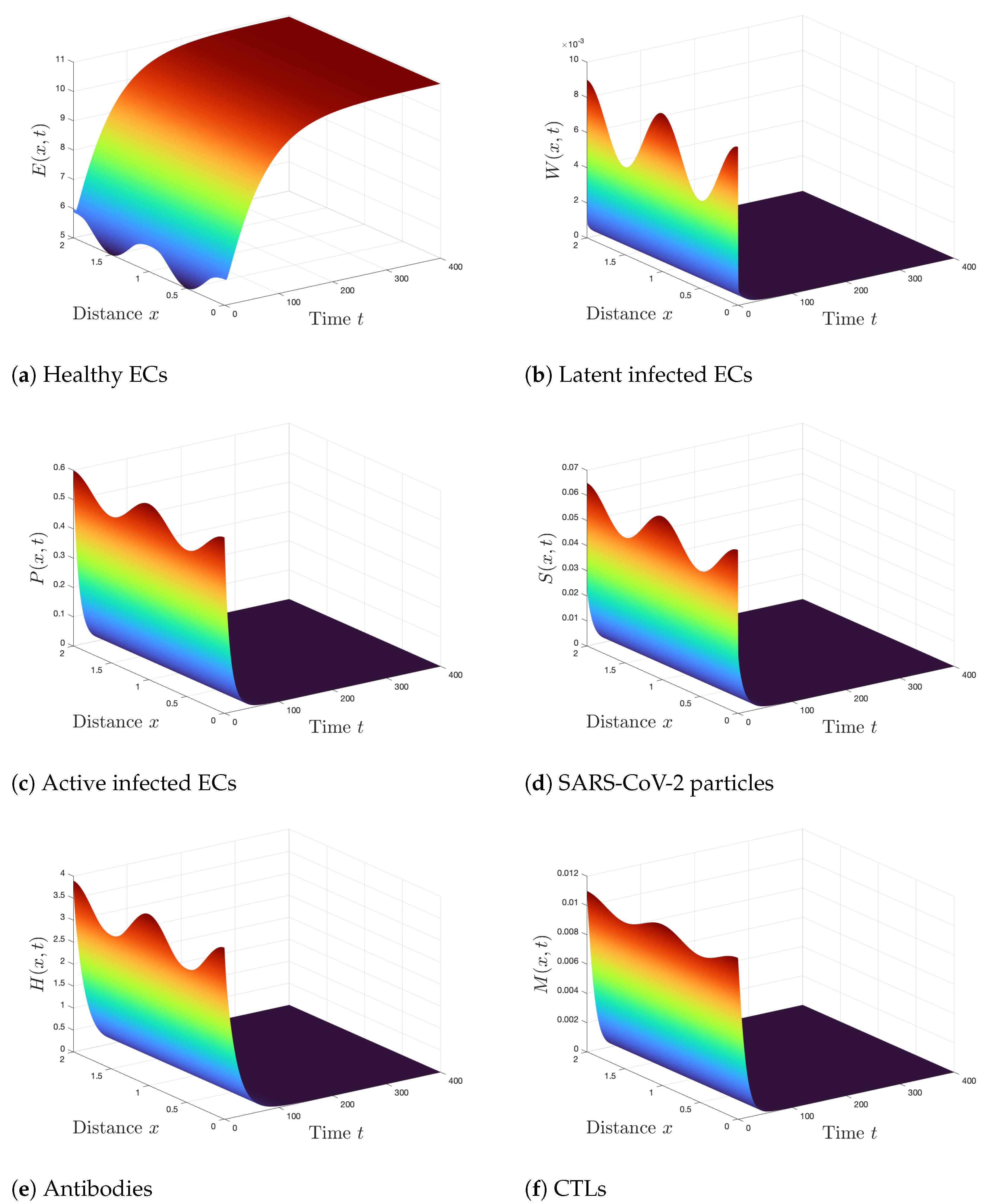
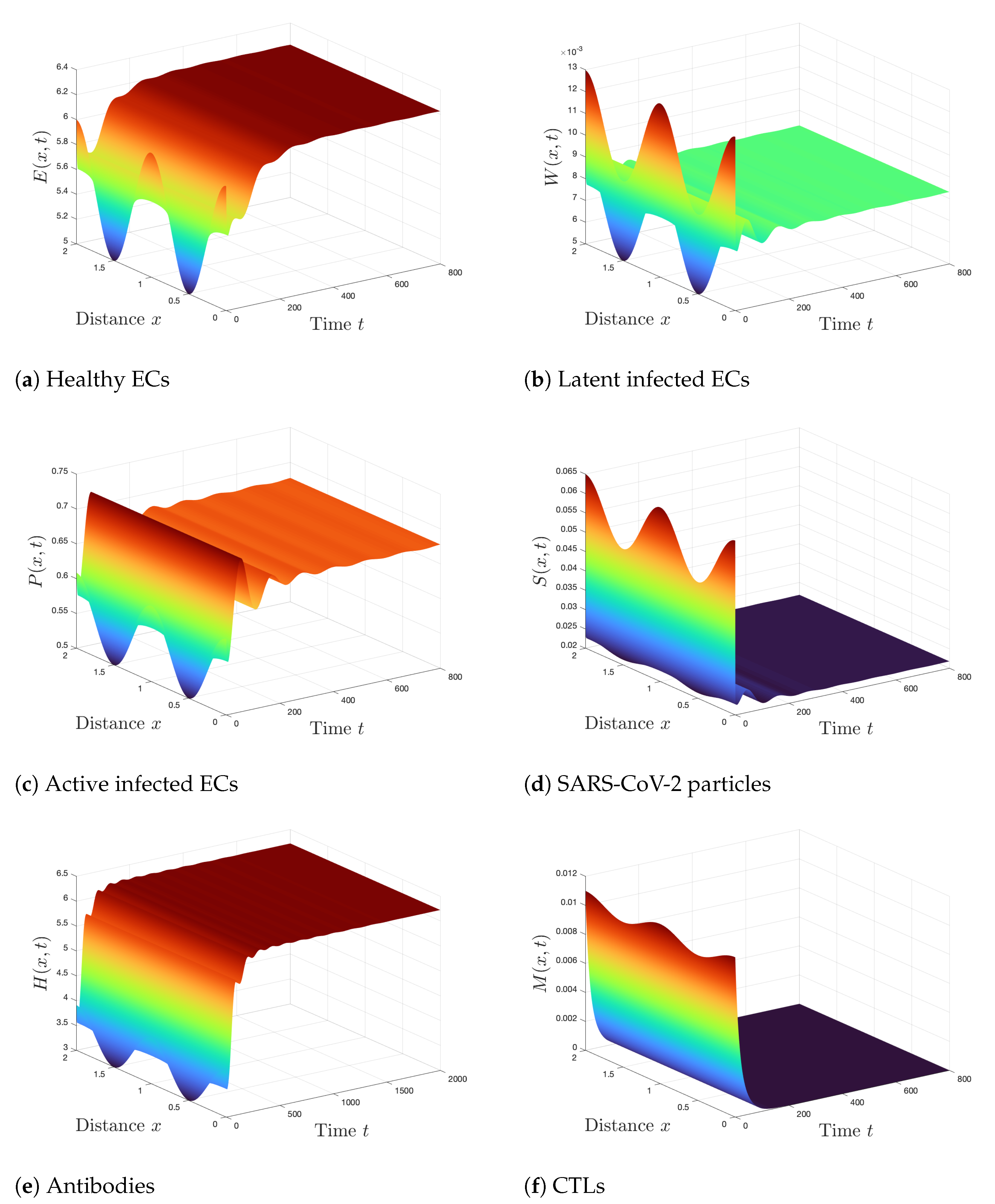
6. Numerical Simulations

In this section, we execute numerical simulations to support the results of Theorems 2–6. The MATLB PDE solver (pdepe) is used to solve Systems (2)–(7). We consider the spatial domain as ϖ = [ 0 , 2 ] , with a step size of 0.02 . The time step size is chosen as 0.1 . Moreover, we consider the following initial conditions:
E ( x , 0 ) = 5 1 + 0.2 cos 2 ( π x ) , W ( x , 0 ) = 0.005 1 + 0.8 cos 2 ( π x ) , P ( x , 0 ) = 0.5 1 + 0.2 cos 2 ( π x ) , S ( x , 0 ) = 0.05 1 + 0.3 cos 2 ( π x ) , H ( x , 0 ) = 3 1 + 0.3 cos 2 ( π x ) , M ( x , 0 ) = 0.01 1 + 0.1 cos 2 ( π x ) , x [ 0 , 2 ] .
In addition, we consider the homogeneous Neumann boundary conditions:
E n = W n = P n = S n = H n = M n = 0 , t > 0 , x = 0 , 2 .
The parameters ( ψ , μ , η ) of Models (2)–(7) are taken as free parameters. The other parameters are fixed, as shown in Table 2. To illustrate the global stability of the five steady states of Models (2)–(7), we have the following cases:
Case 1 (Stability of  S S 0 ): ( ψ , μ , η ) = ( 0.05 , 0.5 , 0.09 ) . For these values, we obtain R 0 = 0.3015 < 1 . According to Theorem 2, S S 0 is GAS and the SARS-CoV-2 infection is predicted to be completely cleared from the body. From Figure 1, we can see that the numerical results agree with the results of Theorem 2. We observe that the concentration of healthy ECs is increased and converged to its normal value E 0 = 10.9495 , whereas the concentrations of other compartments are reducing and tending to zero.
Case 2 (Stability of  S S 1 ): ( ψ , μ , η ) = ( 0.5 , 0.5 , 0.09 ) . Using these values, we compute R 1 H = 0.5332 < 1 , R 1 M = 0.8314 < 1 < R 0 = 3.0146 and β E υ + υ E 1 E m a x = 0.003 > 0 . It means that the conditions of Theorem 3 are valid and thus S S 1 is GAS. From Figure 2, we see that there is an agreement between the numerical simulations and the results of Theorem 3. Further, the states of the system converge to the steady state S S 1 = ( 3.6335 , 0.0109 , 0.8899 , 0.049 , 0 , 0 ) . In this case, the SARS-CoV-2 exists in the body but without any response from the immune system.
Case 3 (Stability of  S S 2 ): ( ψ , μ , η ) = ( 0.5 , 2.3 , 0.09 ) . Consequently, R 1 H = 1.7137 > 1 , R 2 M = 0.6091 < 1 and β E υ + υ E 2 E m a x = 0.0052 > 0 . This shows that the conditions of Theorem 4 are fulfilled and thus S S 2 is GAS. The numerical solutions displayed in Figure 3 are consistent with the results of Theorem 4. Further, the states of the system converge to the steady state S S 2 = ( 6.2268 , 0.0083 , 0.6776 , 0.0218 , 6.2213 , 0 ) . In this case, only the antibody immunity is activated.
Case 4 (Stability of  S S 3 ): ( ψ , μ , η ) = ( 0.5 , 1 , 0.13 ) . We compute R 1 M = 1.1203 > 1 , R 1 H R 2 M = 0.8469 < 1 and β E υ + υ E 3 E m a x = 0.0034 > 0 . According to Theorem 5, S S 3 is GAS and this is shown in Figure 4. We can see that the states of the system converge to the steady state S S 3 = ( 4.0730 , 0.0106 , 0.7713 , 0.0425 , 0 , 0.0150 ) . For this case, the CTLs are activated, whereas the antibody immune response is unstimulated.
Case 5 (Stability of  S S 4 ): ( ψ , μ , η ) = ( 0.5 , 1.6 , 0.13 ) . Hence, we compute R 1 H R 2 M = 1.355 > 1 , R 2 M = 1.0243 > 1 and β E υ + υ E 4 E m a x = 0.0042 > 0 . According to Theorem 6, S S 4 is GAS and this is clarified numerically in Figure 5. The states of the system converge to the steady state S S 4 = ( 5.0433 , 0.0097 , 0.7691 , 0.0313 , 3.0927 , 0.0031 ) . In this situation, both antibodies and CTLs are activated against the viral infection.

7. Discussion

SARS-CoV-2 infection represents a real concern worldwide. Therefore, the modeling and analysis of SARS-CoV-2 are needed to understand the dynamics of this virus within a host. In this paper, we develop a diffusive SARS-CoV-2 infection model with antibody and CTL immune responses. We study the dynamical behavior of the model. We establish that the model has five steady states and we prove the following:
  • The healthy steady state S S 0 always exists and it is GAS when R 0 1 . In this case, the patient will be recoveredfrom COVID-19. From a control viewpoint, making R 0 1 will be a good strategy. This can be obtained by reducing the parameters ψ and ϱ . Let us consider the effect of two types of antiviral drugs, one for blocking the infection with drug efficacy ϵ 1 [ 0 , 1 ] and the other for blocking the production of SARS-CoV-2 with drug efficacy ϵ 2 [ 0 , 1 ] [8]. Modeling the two antiviral drugs will change parameters ψ and ϱ to ( 1 ϵ 1 ) ψ and ( 1 ϵ 2 ) ϱ [21]. Let us consider ϵ 1 = ϵ 2 = ϵ and the other parameters are fixed, then, R 0 can be given as functions of ϵ as follows:
    R 0 ( ϵ ) = ( 1 ϵ ) 2 ϱ ψ E m a x 2 υ β P β S ϑ γ ϑ + β W + 1 γ υ β E + ( υ β E ) 2 + 4 υ ϕ E m a x = ( 1 ϵ ) 2 R 0 ( 0 ) .
    To make R 0 1 , the effectiveness ϵ has to satisfy
    ϵ min ϵ 1 , ϵ min = max 0 , 1 1 R 0 ( 0 ) ,
    where ϵ min is the minimum drug efficacy required to eradicate SARS-CoV-2 from the body.
    We note that R 0 does not depend on the immune response parameters σ , λ , μ , and η . Therefore, both CTL and antibody immune responses can control the viral infection but they do not play the role of clearing the viruses.
  • The infected steady state with inactive immune responses S S 1 exists when R 0 > 1 and β E υ + υ E 1 E m a x > 0 . Further, S S 1 is GAS when R 1 H 1 < R 0 , R 1 M 1 and β E υ + υ E 1 E m a x > 0 . This result suggests that starting from any disease stage, the COVID-19 patient will still have a SARS-CoV-2 infection but without immune responses.
  • The infected steady state with only active antibody immunity S S 2 exists when R 1 H > 1 . Moreover, S S 2 is GAS, when R 1 H > 1 , R 2 M 1 and β E υ + υ E 2 E m a x > 0 . This result suggests that starting from any disease stage, the COVID-19 patient will still have a SARS-CoV-2 infection but with only an active antibody immune response.
  • The infected steady state with only active CTL immunity S S 3 exists when R 1 M > 1 , whereas it is GAS when R 1 M > 1 , R 1 H R 2 M and β E υ + υ E 3 E m a x > 0 . This result suggests that starting from any disease stage, the COVID-19 patient will still have a SARS-CoV-2 infection but with only an active CTL immune response.
  • The infected steady state with both active antibody and CTL immunities S S 4 exists when R 1 H > R 2 M and R 2 M > 1 . Further, S S 4 is GAS when R 1 H > R 2 M > 1 and β E υ + υ E 4 E m a x > 0 . This result suggests that starting from any disease stage, the COVID-19 patient will still have a SARS-CoV-2 infection despite both antibody and CTL immune responses being active.
    We performed the numerical simulations for the model and showed that both the numerical and theoretical results are consistent.
We presented some numerical results and showed that they agreed with the theoretical results. The main limitation of the present work is that we did not validate the model using real data from COVID-19 patients (such as the concentrations of SARS-CoV-2, CTLs, antibodies, etc.). In fact, the real data on SARS-CoV-2 infections are still very limited. Collecting such data from SARS-CoV-2-infected patients is not an easy task and needs further experimental studies.

8. Conclusions

Mathematical models can be helpful for understanding the complex behavior of viral infections and the reaction of the immune system. We noted that the great majority of works on within-host SARS-CoV-2 infection models are based on the assumption that the viruses and cells are homogeneously distributed in the human body. This is a poor approach because the diffusion of viruses and cells causes spatial variations within the body. In this paper, we constructed a diffusive SARS-CoV-2 infection model with antibody and CTL immune responses. The model was given by a system of PDEs that describes the interaction of six compartments: healthy ECs, latent infected ECs, active infected ECs, free SARS-CoV-2 particles, CTLs, and antibodies. We considered a logistic term for healthy ECs. The non-negativity and boundedness of the solutions of the model were proven. Further, we derived four threshold parameters that determine the existence and stability of the five steady states of the model. The global stability of all steady states of the model was investigated by constructing Lyapunov functions and applying LIP. We performed numerical simulations for the model and showed that both the numerical and theoretical results are consistent.
Our model suggest that both CTL and antibody immune responses can play a role in controlling SARS-CoV-2 infection but not in clearing the virus from the body.
We discussed the effect of the antiviral treatment of the SARS-CoV-2 dynamics. Our model can help pharmaceutical companies and biologists to develop effective antiviral drugs for COVID-19 patients that make the basic reproduction number R 0 for patients less than or equal to one. This will lead to the clearance of SARS-CoV-2 from the patient’s body.

Author Contributions

Methodology, A.M.E., A.J.A. and A.D.H.; Formal analysis, A.M.E.; Investigation, A.M.E., A.J.A. and S.A.A.; Writing—original draft, A.J.A. and A.D.H.; Writing—review an editing, S.A.A. All authors have read and agreed to the published version of the manuscript.

Funding

This project was funded by the Deanship of Scientific Research (DSR), King Abdulaziz University, Jeddah, Saudi Arabia, under grant no. KEP-PHD-95-130-42.

Data Availability Statement

Not applicable.

Acknowledgments

This project was funded by the Deanship of Scientific Research (DSR), King Abdulaziz University, Jeddah, Saudi Arabia, under grant no. KEP-PHD-95-130-42. The authors, therefore, acknowledge with thanks the DSR’s technical and financial support.

Conflicts of Interest

The authors declare no conflict of interest.

References

  1. Olaniyi, S.; Obabiyi, O.S.; Okosun, K.O.; Oladipo, A.T.; Adewale, S.O. Mathematical modelling and optimal cost-effective control of COVID-19 transmission dynamics. Eur. J. Plus 2020, 135, 938. [Google Scholar] [CrossRef] [PubMed]
  2. Asamoah, J.K.K.; Okyere, E.; Abidemi, A.; Moore, S.E.; Sun, G.Q.; Jin, Z.; Acheampong, E.; Gordon, J.F. Optimal control and comprehensive cost-effectiveness analysis for COVID-19. Results Phys. 2022, 33, 105177. [Google Scholar] [CrossRef] [PubMed]
  3. Coronavirus Disease (COVID-19), Vaccine Tracker, World Health Organization (WHO). 2022. Available online: https://covid19.trackvaccines.org/agency/who/ (accessed on 1 December 2022).
  4. Nowak, M.D.; Sordillo, E.M.; Gitman, M.R.; Mondolfi, A.E. Coinfection in SARS-CoV-2 infected patients: Where are influenza virus and rhinovirus/enterovirus? J. Med. Virol. 2020, 92, 1699. [Google Scholar] [CrossRef]
  5. Hernandez-Vargas, E.A.; Wilk, E.; Canini, L.; Toapanta, F.R.; Binder, S.C.; Uvarovskii, A.; Ross, T.M.; Guzmán, C.A.; Perelson, A.S.; Meyer-Hermann, M. Effects of aging on influenza virus infection dynamics. J. Virol. 2014, 88, 4123–4131. [Google Scholar] [CrossRef] [Green Version]
  6. Murphy, K. SARS CoV-2 detection from upper and lower respiratory tract specimens: Diagnostic and infection control implications. Chest 2020, 158, 1804–1805. [Google Scholar]
  7. Varga, Z.; Flammer, A.J.; Steiger, P.; Haberecker, M.; Andermatt, R.; Zinkernagel, A.S.; Mehra, M.R.; Schuepbach, R.A.; Ruschitzka, F.; Moch, H. Endothelial cell infection and endotheliitis in COVID-19. Lancet 2020, 395, 1417–1418. [Google Scholar] [CrossRef]
  8. Hernandez-Vargas, E.A.; Velasco-Hernandez, J.X. In-host mathematical modelling of COVID-19 in humans. Annu. Rev. Control 2020, 50, 448–456. [Google Scholar] [CrossRef]
  9. Li, C.; Xu, J.; Liu, J.; Zhou, Y. The within-host viral kinetics of SARS-CoV-2. Math. Biosci. Eng. 2020, 17, 2853–2861. [Google Scholar] [CrossRef]
  10. Gonçalves, A.; Bertrand, J.; Ke, R.; Comets, E.; De Lamballerie, X.; Malvy, D.; Pizzorno, A.; Terrier, O.; Rosa Calatrava, M.; Mentré, F.; et al. Timing of antiviral treatment initiation is critical to reduce SARS-CoV-2 viral load. CPT Pharmacometrics Syst. Pharmacol. 2020, 9, 509–514. [Google Scholar] [CrossRef]
  11. Abuin, P.; Anderson, A.; Ferramosca, A.; Hernandez-Vargas, E.A.; Gonzalez, A.H. Characterization of SARS-CoV-2 dynamics in the host. Annu. Rev. Control. 2020, 50, 457–468. [Google Scholar] [CrossRef]
  12. Chhetri, B.; Bhagat, V.M.; Vamsi, D.K.K.; Ananth, V.S.; Prakash, D.B.; Mandale, R.; Muthusamy, S.; Sanjeevi, C.B. Within-host mathematical modeling on crucial inflammatory mediators and drug interventions in COVID-19 identifies combination therapy to be most effective and optimal. Alex. Eng. J. 2021, 60, 2491–2512. [Google Scholar] [CrossRef]
  13. Elaiw, A.M.; Alsaedi, A.J.; Agha, A.D.A.; Hobiny, A.D. Global stability of a humoral immunity COVID-19 model with logistic growth and delays. Mathematics 2022, 10, 1857. [Google Scholar] [CrossRef]
  14. Tay, M.Z.; Poh, C.M.; Rénia, L.; MacAry, P.A.; Ng, L.F. The trinity of COVID-19: Immunity, inflammation and intervention. Nat. Rev. Immunol. 2020, 20, 363–374. [Google Scholar] [CrossRef]
  15. Ren, X.; Wen, W.; Fan, X.; Hou, W.; Su, B.; Cai, P.; Li, J.; Liu, Y.; Tang, F.; Zhang, F.; et al. COVID-19 immune features revealed by a large-scale single-cell transcriptome atlas. Cell 2021, 184, 1895–1913. [Google Scholar] [CrossRef]
  16. Shah, V.K.; Firmal, P.; Alam, A.; Ganguly, D.; Chattopadhyay, S. Overview of immune response during SARS-CoV-2 infection: Lessons from the past. Front. Immunol. 2020, 11, 1949. [Google Scholar] [CrossRef] [PubMed]
  17. Quast, I.; Tarlinton, D. B cell memory: Understanding COVID-19. Immunity 2021, 54, 205–210. [Google Scholar] [CrossRef]
  18. Alzahrani, T. Spatio-temporal modeling of immune response to SARS-CoV-2 infection. Mathematics 2021, 9, 3274. [Google Scholar] [CrossRef]
  19. Ke, R.; Zitzmann, C.; Ho, D.D.; Ribeiro, R.M.; Perelson, A.S. In vivo kinetics of SARS-CoV-2 infection and its relationship with a person’s infectiousness. Proc. Natl. Acad. Sci. USA 2021, 118, e2111477118. [Google Scholar] [CrossRef]
  20. Sadria, M.; Layton, A.T. Modeling within-host SARS-CoV-2 infection dynamics and potential treatments. Viruses 2021, 13, 1141. [Google Scholar] [CrossRef]
  21. Ghosh, I. Within host dynamics of SARS-CoV-2 in humans: Modeling immune responses and antiviral treatments. SN Comput. Sci. 2021, 2, 482. [Google Scholar] [CrossRef]
  22. Du, S.Q.; Yuan, W. Mathematical modeling of interaction between innate and adaptive immune responses in COVID-19 and implications for viral pathogenesis. J. Med. Virol. 2020, 92, 1615–1628. [Google Scholar] [CrossRef] [PubMed]
  23. Hattaf, K.; Yousfi, N. Dynamics of SARS-CoV-2 infection model with two modes of transmission and immune response. Math. Biosci. Eng. 2020, 17, 5326–5340. [Google Scholar] [CrossRef] [PubMed]
  24. Mondal, J.; Samui, P.; Chatterjee, A.N. Dynamical demeanour of SARS-CoV-2 virus undergoing immune response mechanism in COVID-19 pandemic. Eur. Phys. J. Spec. Top. 2022, 1–14. [Google Scholar] [CrossRef]
  25. Almoceraa, A.E.S.; Quiroz, G.; Hernandez-Vargas, E.A. Stability analysis in COVID-19 within-host model with immune response. Commun. Nonlinear Sci. Numer. Simul. 2021, 95, 105584. [Google Scholar] [CrossRef]
  26. Nath, B.J.; Dehingia, K.; Mishra, V.N.; Chu, Y.-M.; Sarmah, H.K. Mathematical analysis of a within-host model of SARS-CoV-2. Adv. Differ. Equations 2021, 2021, 113. [Google Scholar] [CrossRef]
  27. Agha, A.D.A.; Elaiw, A.M.; Ramadan, S.A.A.E. Stability analysis of within-host SARS-CoV-2/HIV coinfection model. Math. Methods Appl. Sci. 2022, 45, 11403–11422. [Google Scholar] [CrossRef]
  28. Elaiw, A.M.; Alsulami, R.S.; Hobiny, A.D. Modeling and stability analysis of within-host IAV/SARS-CoV-2 coinfection with antibody immunity. Mathematics 2022, 10, 4382. [Google Scholar] [CrossRef]
  29. Wodarz, D.; Christensen, J.P.; Thomsen, A.R. The importance of lytic and nonlytic immune responses in viral infections. Trends Immunol. 2002, 23, 194–200. [Google Scholar] [CrossRef]
  30. Agha, A.D.A.; Elaiw, A.M. Global dynamics of SARS-CoV-2/malaria model with antibody immune response. Math. Biosci. Eng. 2022, 19, 8380–8410. [Google Scholar] [CrossRef]
  31. Elaiw, A.M.; Agha, A.D.A.; Alshaikh, M.A. Global stability of a within-host SARS-CoV-2/cancer model with immunity and diffusion. Int. J. Biomath. 2022, 15, 2150093. [Google Scholar] [CrossRef]
  32. Elaiw, A.M.; Agha, A.D.A. Global Stability of a reaction-diffusion malaria/COVID-19 coinfection dynamics model. Mathematics 2022, 10, 4390. [Google Scholar] [CrossRef]
  33. Xu, Z.; Xu, Y. Stability of a CD4+ T cell viral infection model with diffusion. Int. J. Biomath. 2018, 11, 1850071. [Google Scholar] [CrossRef]
  34. Zhang, Y.; Xu, Z. Dynamics of a diffusive HBV model with delayed Beddington-DeAngelis response. Nonlinear Anal. Real World Appl. 2014, 15, 118–139. [Google Scholar] [CrossRef]
  35. Smith, H.L. Monotone Dynamical Systems: An Introduction to the Theory of Competitive and Cooperative Systems; American Mathematical Society: Providence, RI, USA, 1995. [Google Scholar]
  36. Protter, M.H.; Weinberger, H.F. Maximum Principles in Differential Equations; Prentic Hall: Englewood Cliffs, NJ, USA, 1967. [Google Scholar]
  37. Henry, D. Geometric Theory of Semilinear Parabolic Equations; Springer-Verlag: New York, NY, USA, 1993. [Google Scholar]
  38. Korobeinikov, A. Global properties of basic virus dynamics models. Bull. Math. Biol. 2004, 66, 879–883. [Google Scholar] [CrossRef]
  39. Khalil, H.K. Nonlinear Systems; Pearson Education: Boston, MA, USA; Prentice Hall: Englewood Cliffs, NJ, USA, 2002. [Google Scholar]
Figure 1. Simulation of Systems (2)–(7) when ( ψ , μ , η ) = ( 0.05 , 0.5 , 0.09 ) . The steady state S S 0 ( 10.9495 , 0 , 0 , 0 , 0 , 0 ) is GAS.
Mathematics 11 00190 g001
Figure 2. Simulation of Systems (2)–(7) when ( ψ , μ , η ) = ( 0.5 , 0.5 , 0.09 ) . The steady state S S 1 = ( 3.6335 , 0.0109 , 0.8899 , 0.049 , 0 , 0 ) is GAS.
Mathematics 11 00190 g002
Figure 3. Simulation of Systems (2)–(7) when ( ψ , μ , η ) = ( 0.5 , 2.3 , 0.09 ) . The steady state S S 2 = ( 6.2268 , 0.0083 , 0.6776 , 0.0218 , 6.2213 , 0 ) is GAS.
Mathematics 11 00190 g003
Figure 4. Simulation of Systems (2)–(7) when ( ψ , μ , η ) = ( 0.5 , 1 , 0.13 ) . The steady state S S 3 = ( 4.0730 , 0.0106 , 0.7713 , 0.0425 , 0 , 0.0150 ) is GAS.
Mathematics 11 00190 g004
Figure 5. Simulation of Systems (2)–(7) when ( ψ , μ , η ) = ( 0.5 , 1.6 , 0.13 ) . The steady state S S 4 = ( 5.0433 , 0.0097 , 0.7691 , 0.0313 , 3.0927 , 0.0031 ) is GAS.
Mathematics 11 00190 g005
Table 1. Steady states and their global stability conditions for Models (2)–(7).
Steady StateGlobal Stability Conditions
S S 0 = ( E 0 , 0 , 0 , 0 , 0 , 0 ) R 0 1
S S 1 = ( E 1 , W 1 , P 1 , S 1 , 0 , 0 ) R 1 H 1 < R 0 , R 1 M 1 and β E υ + υ E 1 E m a x > 0
S S 2 = ( E 2 , W 2 , P 2 , S 2 , H 2 , 0 ) R 1 H > 1 , R 2 M 1 and β E υ + υ E 2 E m a x > 0
S S 3 = ( E 3 , W 3 , P 3 , S 3 , 0 , M 3 ) R 1 M > 1 , R 1 H R 2 M and β E υ + υ E 3 E m a x > 0
S S 4 = ( E 4 , W 4 , P 4 , S 4 , H 4 , M 4 ) R 1 H > R 2 M > 1 and β E υ + υ E 4 E m a x > 0
Table 2. Model parameters.
ParameterValueParameterValueParameterValueParameterValue
ϕ 0.1 σ 0.8 β W 0.001 D W 0.01
υ 0.01 ϱ 0.24 β P 0.1 D P 0.01
E max 12 λ 0.5 β S 4.36 D S 0.01
ψ varied μ varied β H 0.05 D H 0.01
γ 0.5 η varied β M 0.1 D M 0.01
ϑ 4.08 β E 0.01 D E 0.01
Disclaimer/Publisher’s Note: The statements, opinions and data contained in all publications are solely those of the individual author(s) and contributor(s) and not of MDPI and/or the editor(s). MDPI and/or the editor(s) disclaim responsibility for any injury to people or property resulting from any ideas, methods, instructions or products referred to in the content.

