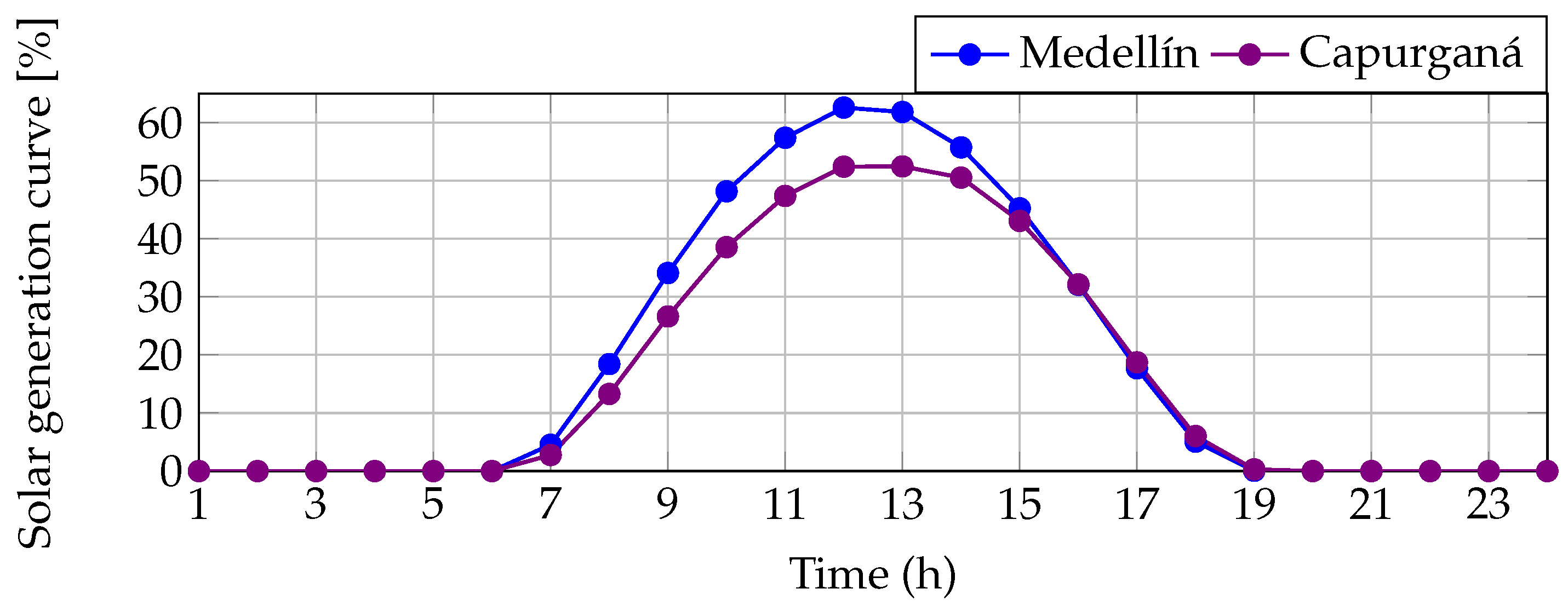
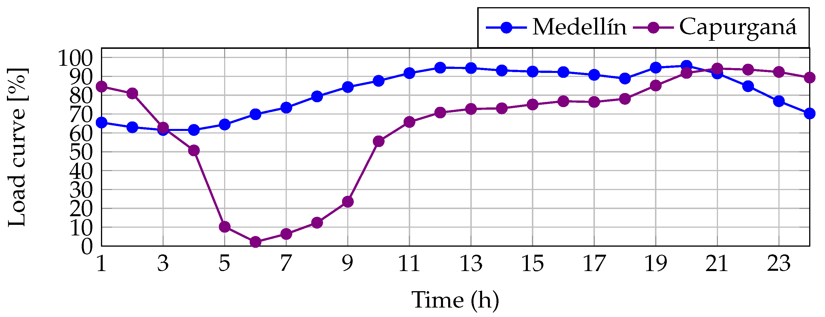
This section shows, analyzes, and discuses all results obtained by the optimization algorithms to solve the problem of optimal operation of PV distributed generators in DC networks. To accomplish this task, we employed a grid-connected and a standalone grid from Medellín and Capurganá in Colombia, respectively. To realize all the simulations, we used the numerical computing system Matlab 2022a version, by using a Dell Precision 3450 workstation with an Intel(R) Core(TM) i9-11900
[email protected] GHz and 64.0 GB RAM running Windows 10 Pro 64-bit. Finally, each algorithm was executed 100 times for each objective function, with the intention of evaluating the average solution for each index used, the standard deviation, and the average processing times required by the optimization methodologies.
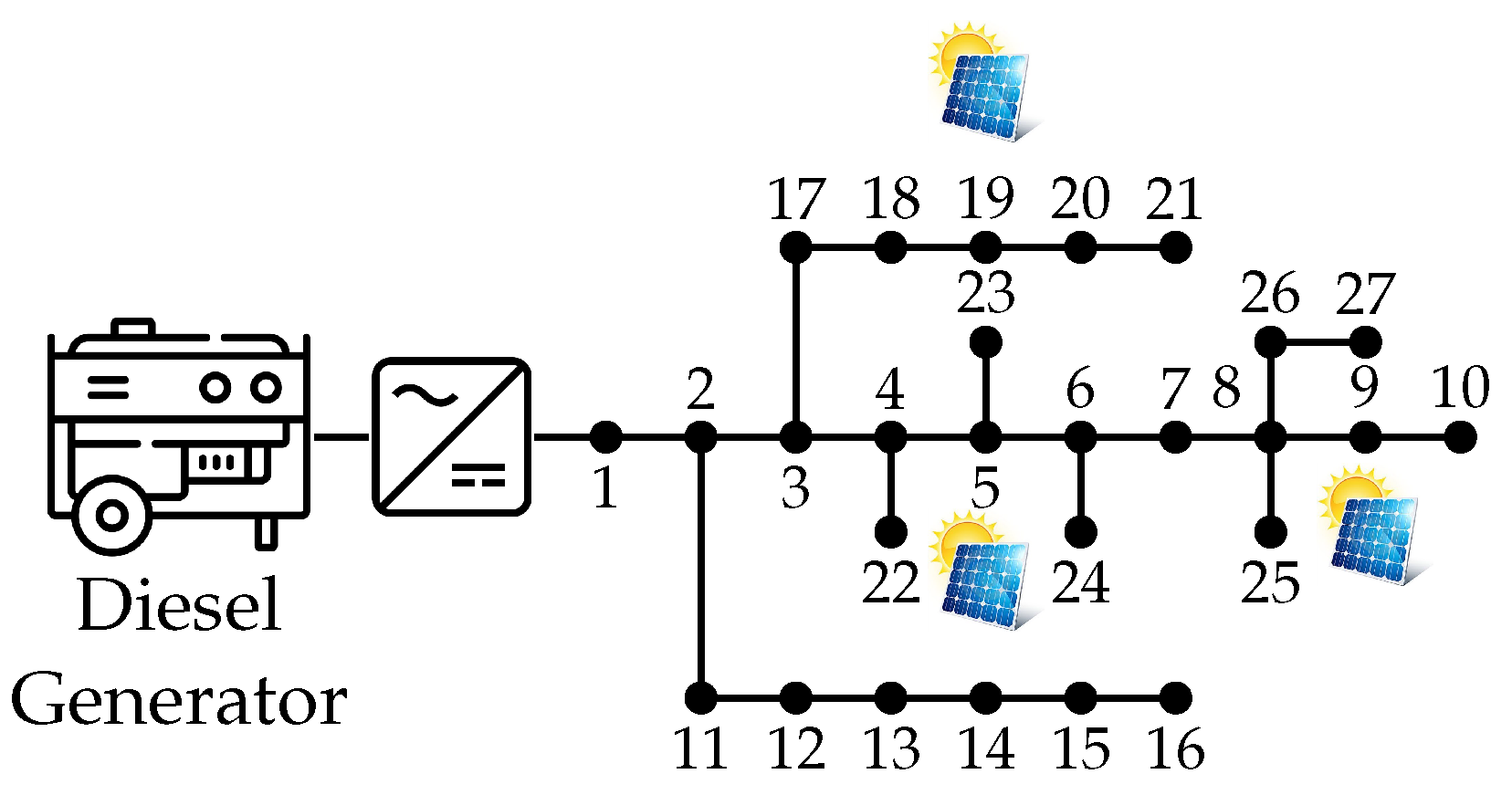
5.1. Capurganá’s Network: Standalone System
Table 9 presents all simulation results obtained for the different optimization methods for each objective function used. This table is arranged from left to right as follows: the first column corresponds to the optimization algorithm employed. In the second, third, and fourth columns, we present the results related to the objective functions that we are seeking to minimize in this document (
,
, and
), where
is the energy losses in the grid associated with the energy transport in
,
is the energy purchasing cost of the conventional generators located in the DC grid in USD, and
is the
emission related to the energy production in the DC grid by the conventional generators in
. In the first row of this table, we present the values associated with the electrical network without PV distributed generation (base case) for each objective function. The rest of the table continues with the analysis of the average solution obtained by each solution methodology, the percentage of reduction with respect to the base case, the standard deviation obtained by each method, and the average processing time that it took each algorithm to reach the presented solution.
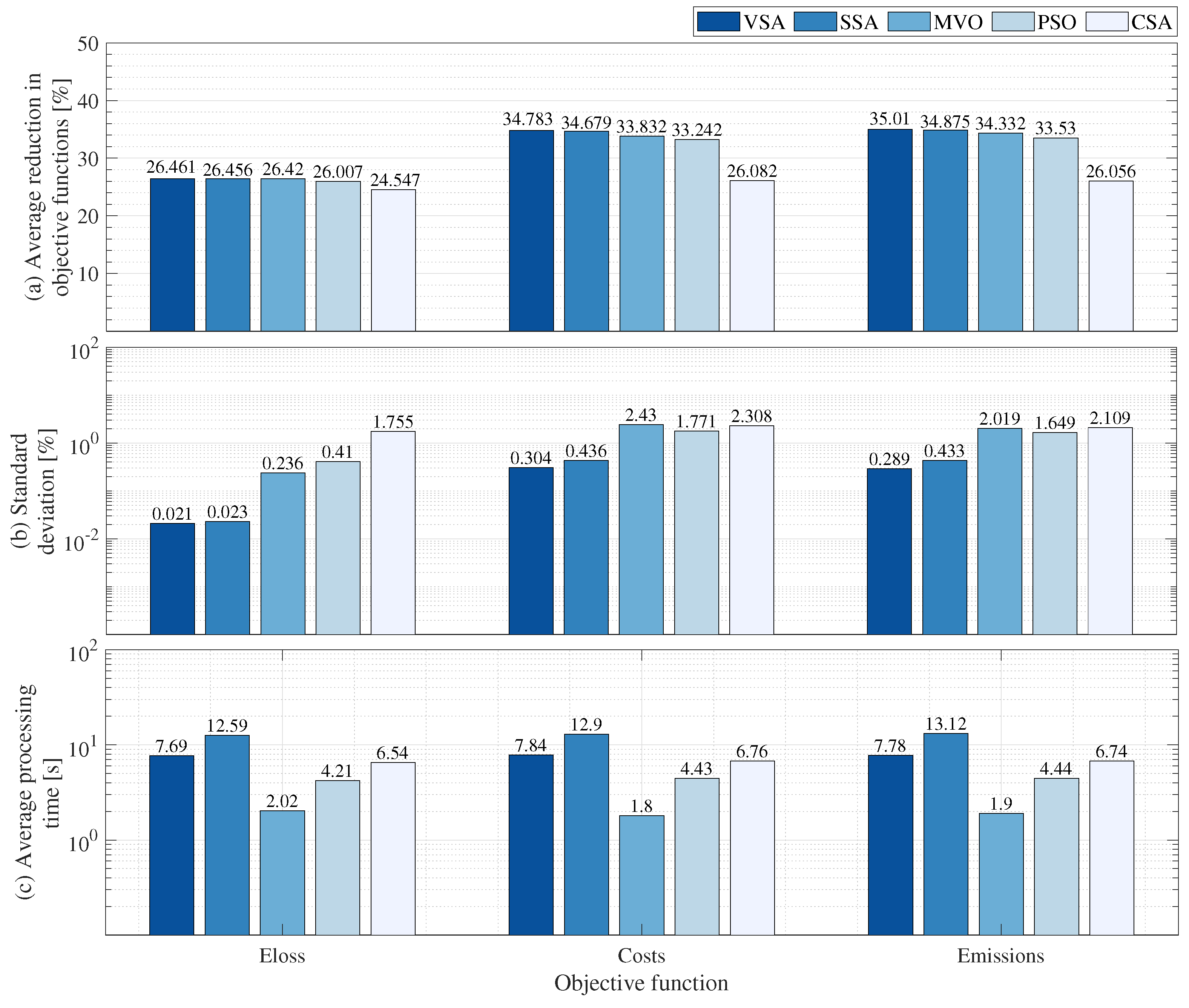
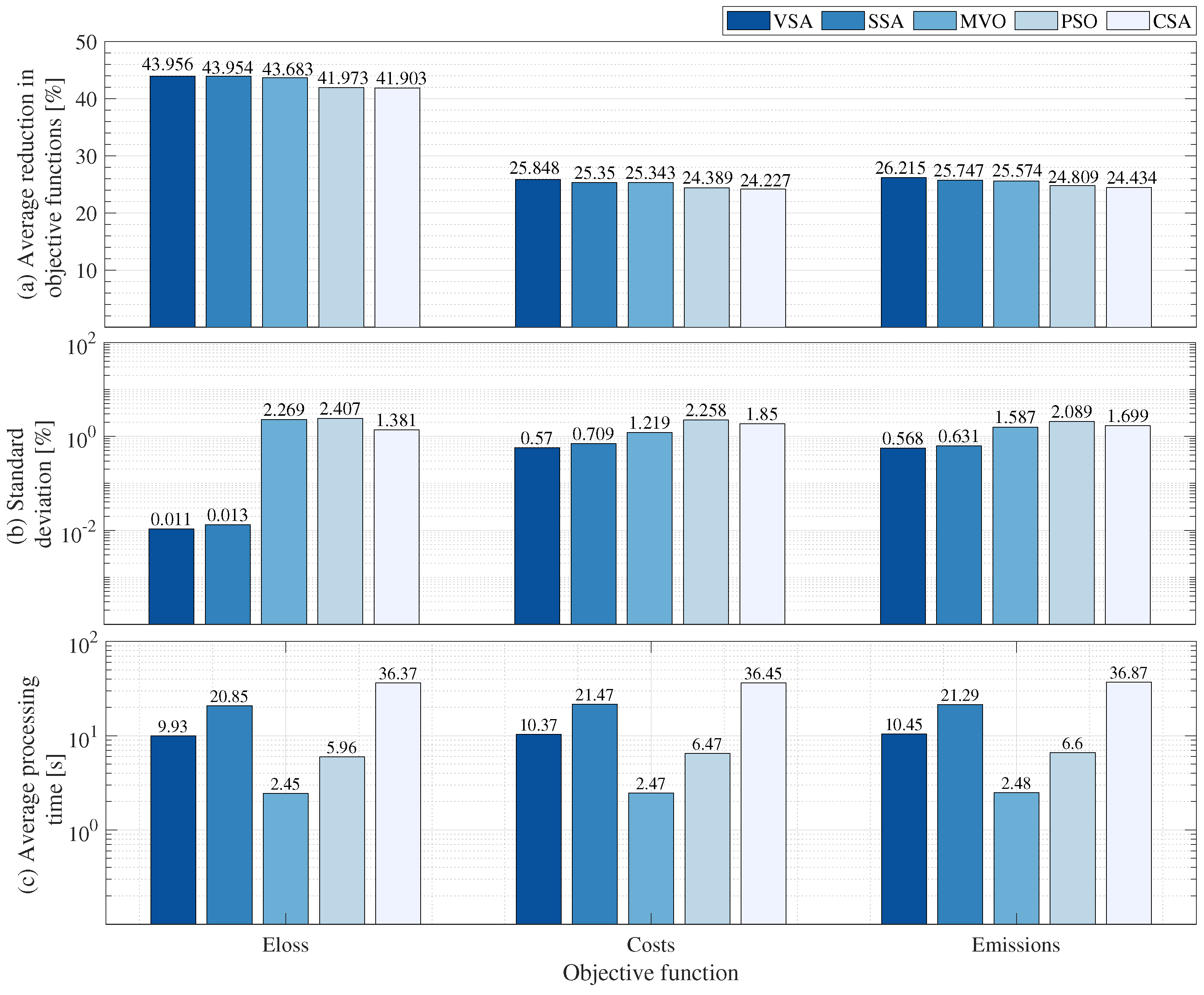
By analyzing the results obtained in the last table, it is possible to obtain
Figure 7. This figure shows the percentage of average reduction by each method (a) with respect to base case, the percentage of standard deviation reached by each algorithm (b), and the average processing time that each algorithm needs to obtain the solution for the problem addressed, in seconds (c). In
Figure 7a, we analyze the percentage of average reduction obtained by the optimization algorithms for each objective function. For the
case, the VSA algorithm obtains an
of
, achieving a reduction of
, outperforming SSA by
, MVO by
, PSO by
, and CSA by
. For the
case, the proposed algorithm obtains a percentage reduction of
, reaching an
value of
, outperforming the other methodologies by an average percentage of
. In the
case, the VSA once again obtains the best solution, reaching an
value of
, and reaching an emissions average percentage reduction of
in relation to the base case, outperforming SSA, MVO, PSO, and CSA by
,
,
, and
, respectively. The discussion presented shows that the VSA obtains the best average solutions for the three objective functions addressed in this document.
Figure 7b compares the solutions obtained by each optimization algorithm in terms of standard deviation in the
,
, and
objective functions. In the first one, the VSA algorithm obtains a percentage of standard deviation of
, beating SSA by
, MVO by
, PSO by
, and CSA by
. In the second case, related to the
, the VSA occupies the first position, with a minor standard deviation percentage (
), outperformingSSA, PSO, CSA, and MVO by
,
,
, and
, respectively. In the third case, associated with reduction of
, the proposed algorithm reaches a standard deviation value of
, outperforming the other algorithms by an average percentage of
. Thus, through the results obtained from
Figure 7b, it is possible to observe the excellent accuracy of the VSA in terms of repeatability for standalone grids; it outperforms the other optimization algorithms in each of the objective functions used in this document, and reaches excellent-quality solutions every time the algorithm is executed.
Figure 7c compares the average time employed by each method to obtain the solution for each objective function used. In the
case, the VSA algorithm obtains an average processing time of
, being surpassed by the MVO, PSO, and CSA algorithms, which obtain
,
, and
, respectively, with the proposed methodology being faster than the SSA algorithm, which requires an average time of
. In the
case, the proposed algorithm reaches an average processing time of
, requiring more time than the MVO, PSO, and CSA algorithms, which obtain
,
, and
, but surprisingly less time than the SSA algorithm, which reaches a
average time value. In the
case, the VSA algorithm obtains an average processing time of
, beating the MVO, PSO, and CSA algorithms by
,
, and
; reducing the processing time required by the SSA algorithm by
. Although the VSA algorithm does not have the shortest processing time, it is important to note that the proposed algorithm takes only
seconds on average to reach the best average solution to solve the problem addressed in the
,
, and
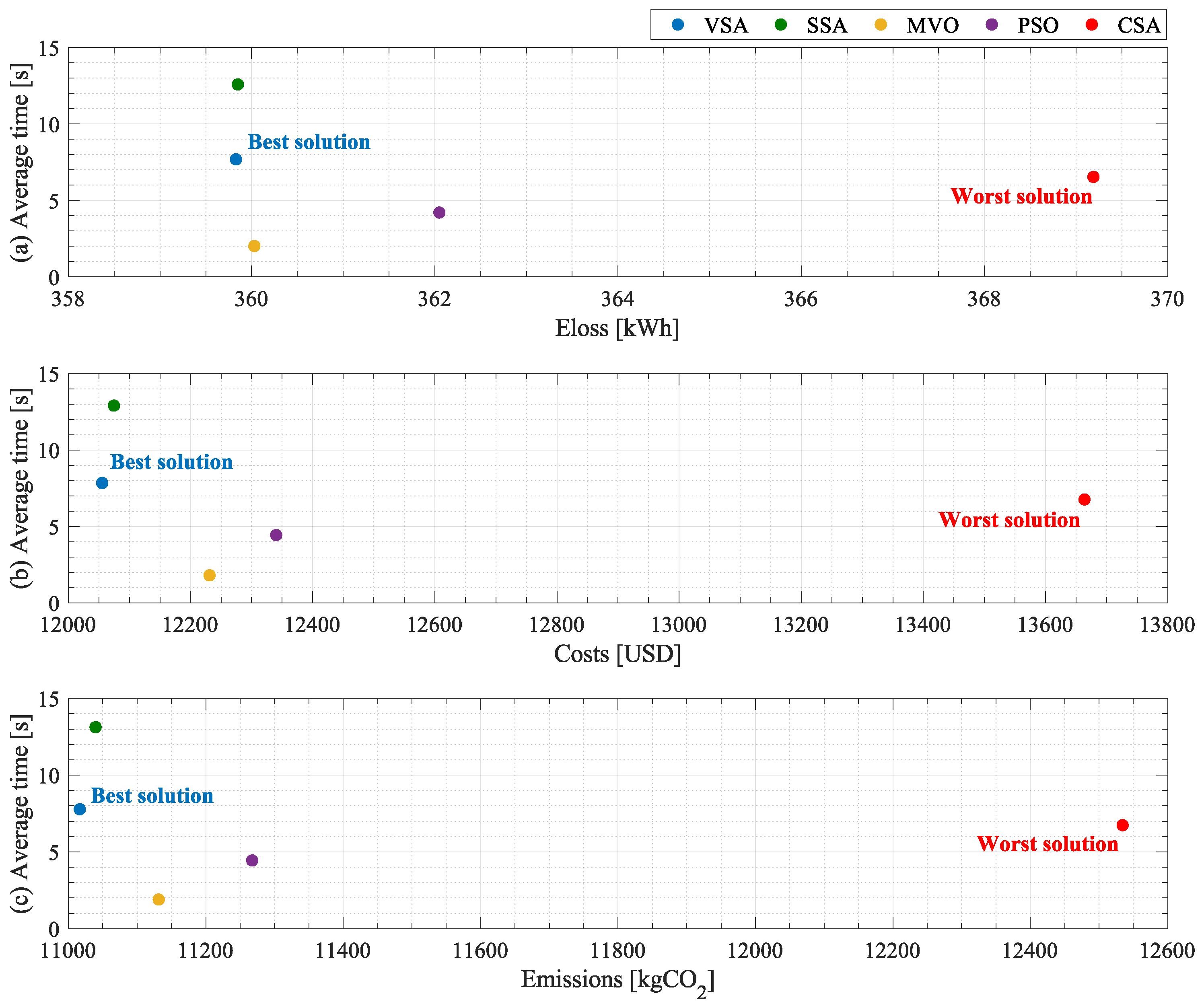
objective functions for a whole operation day, which is a reduced time in terms of grid operation. However, to demonstrate that the VSA algorithm is the method with the best trade-off between solution quality and processing time for solving the problem of optimal operation of PV distributed generators in standalone DC networks,
Table 10 is presented.
The previous table is arranged from left to right as follows: the optimization algorithm and the objective function results, ordering the results with the aim to present the average solution obtained and processing time; presenting, at the end, the distance with respect to the origin (
point) which graphically represents the best solution to the problem in
Figure 8. It represents 0
(
Figure 8a), 0
(
Figure 8b), and 0
(
Figure 8c) with a
processing time requirement, with respect to all scenarios generated by the different objective functions used. In
Figure 8, we fix the
x-axis to the objective function analyzed, and on the
y-axis is the average processing time required by each solution methodology. It is important to mention that to calculate the distance from the origin to the optimization algorithms, the Pythagorean theorem was used, by considering the objective function and the average processing time data.
Table 10 and
Figure 8 demonstrate that the VSA optimization algorithm is the technique that obtains the best trade-off between average solution and processing time for the different objective functions used. In all scenarios, the VSA achieved the minor distance with respect to the origin, which means that the VSA obtained the minor objective function value and processing time. This shows that the proposed methodology has an excellent impact on the solution quality for the problem of optimal operation of PV distributed generators in standalone DC networks in each of the objective functions, by presenting reduced processing time. Therefore, the VSA algorithm is the technique that allows to obtain the best results when technical, economical, and environmental indexes are analyzed and the processing time required is considered for an isolated network.
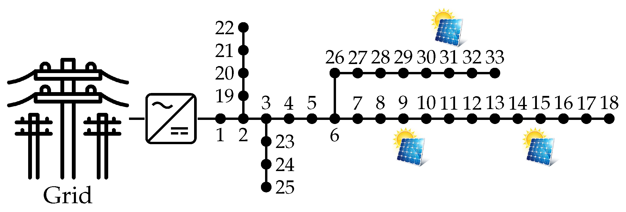
5.2. Medellín’s Network: Grid-Connected System
In this subsection, we analyze the results obtained by all optimization algorithms in the grid-connected system studied. To achieve this,
Table 11 is arranged in the same form as
Table 9. In the first row of this table, we present values obtained in the test system without considering the inject of PV power by the DGs in relation to the
,
, and
, respectively. The analysis continues, showing the results obtained by each algorithm in terms of average solution, percentage of average reduction obtained by each solution methodology with respect to the base case, the standard deviation obtained by each method, and, finally, analyzing the average processing time required by each optimization algorithm after 1000 executions.
By analyzing the results described in this table, it is possible to obtain
Figure 9, where the results achieved by each algorithm are shown. This figure illustrates the percentage of reduction with respect to base case (
Figure 9a), the percentage of standard deviation obtained by each algorithm (
Figure 9b), and the average processing time required to reach the average solution (
Figure 9c) in relation to the objective functions used.
In relation to the reductions obtained with respect to the base case, in the particular case of energy losses,
Figure 9a shows that the VSA algorithm reaches a reduction in average
of
, outperforming the SSA by
, MVO by
, PSO by
, and the CSA by
. In the costs stage, the proposed algorithm obtains an
value of
, reducing
with respect to base case, outperforming the SSA, MVO, PSO, and CSA algorithms by
,
,
, and
, respectively. In the case of emissions, the VSA method obtains an
value of 12,345.1497, ranking as the algorithm that achieves the best reduction with a percentage of
, outperforming the other techniques by an average percentage of
. The last discussion demonstrates that the VSA algorithm allows obtaining the best average reduction for solving the optimal operation problem of distributed photovoltaic generators in DC grids, allowing the grid operator to perform the most optimal grid planning for a day of operation in technical, economical, and environmental terms for grid-connected networks.
To evaluate the accuracy presented by each algorithm,
Figure 9b is presented. This figure compares the standard deviation obtained by each method to solve the problem of optimal operation of PV distributed generators in grid-connected DC networks in the three objective functions. In the energy losses case, the VSA algorithm obtains the best percentage of standard deviation with a value of
, outperforming the other algorithms by an average percentage of
. By analyzing the objective function related to the energy costs, the VSA ranks first, with a standard deviation percentage of
, beating SSA by
, MVO by
, CSA by
, and PSO by
. In the emissions case, once again, the VSA obtains the best percentage of standard deviation with a value of
, ranking as the best solution methodology with an average reduction of
. These results show excellence in terms of solution quality and repeatability of the proposed algorithm in grid-connected networks.
Finally, with the intention of analyzing the processing time required by the solutions,
Figure 9c is presented. This figure compares the average processing time required by each optimization algorithm. In the
terms, the VSA is positioned third, with an average processing time of
s, behind the MVO and the PSO, which obtain times of 2.45 s and 5.96 s, respectively, and reducing the timesreported by SSA and CSA, which are positioned fourth and fifth, with average processing times of 20.85 s and 36.37 s. In the
case, the VSA algorithm is outperformed by MVO and PSO just by 7.9 s and 3.9 s, respectively, but the VSA reduces the processing time reported by the SSA by 11.09 s and the CSA by 26.07 s. In the analysis of
, the VSA ranked third behind the MVO and PSO just by 7.97 s and 3.85 s, but outperformed SSA and CSA by 10.85 s and 26.42 s. The average processing times discussed above show that the fastest optimization algorithms are MVO and PSO; however, these algorithms become stuck in local optima because not enough processing time is used in the exploration phase. On the other hand, the VSA has more adequate exploration and exploitation phases in comparison with the other optimization algorithms, allowing it to escape from local optima and find solutions of high quality in lower processing times, for each objective function employed.
Finally, for a standalone network, with the aim to identify the optimization algorithm with the best trade-off between solution quality and processing time,
Table 12 is presented. This table is arranged in the same order as
Table 10. Through this table, is possible to obtain
Figure 10, where the average solution of each objective function vs. average processing time are plotted, by again considering the solution with the minor distance to the origin as the best solution methodology.
The results plotted in
Figure 10 demonstrate that the VSA had the capacity to solve the problem of optimal operation of PV DGs in grid-connected in DC networks with the best trade-off between technical, economical, and environmental stages, and processing times. These results allow the network operator to perform operation of a grid-connected system in shorter processing times, achieving large reductions in energy losses, operating costs, and power purchases from the grid, and also greatly reducing greenhouse gas emissions to the environment.


 ,
, 


