
Comparing Neural Style Transfer and Gradient-Based Algorithms in Brushstroke Rendering Tasks
 , , , , and
Abstract
:1. Introduction
- a method for quantifying brushstroke rendering results based on correlation analysis of feature histograms,
2. Related Work
Methods for Evaluating the Effectiveness of NPR Algorithms
3. Materials and Methods
3.1. Neural Style Transfer with Explicit Brushstrokes
3.2. Gradient Algorithm for Brushstroke Rendering
| Algorithm 1 Gradient-Based Brushstroke Rendering |
 |
3.3. Brushstroke Features
- Length. Brushstroke length along the skeleton of the brushstroke. For each brushstroke, consisting of N pixels with coordinates , , , the length is calculated as the sum of the distances between neighboring points:
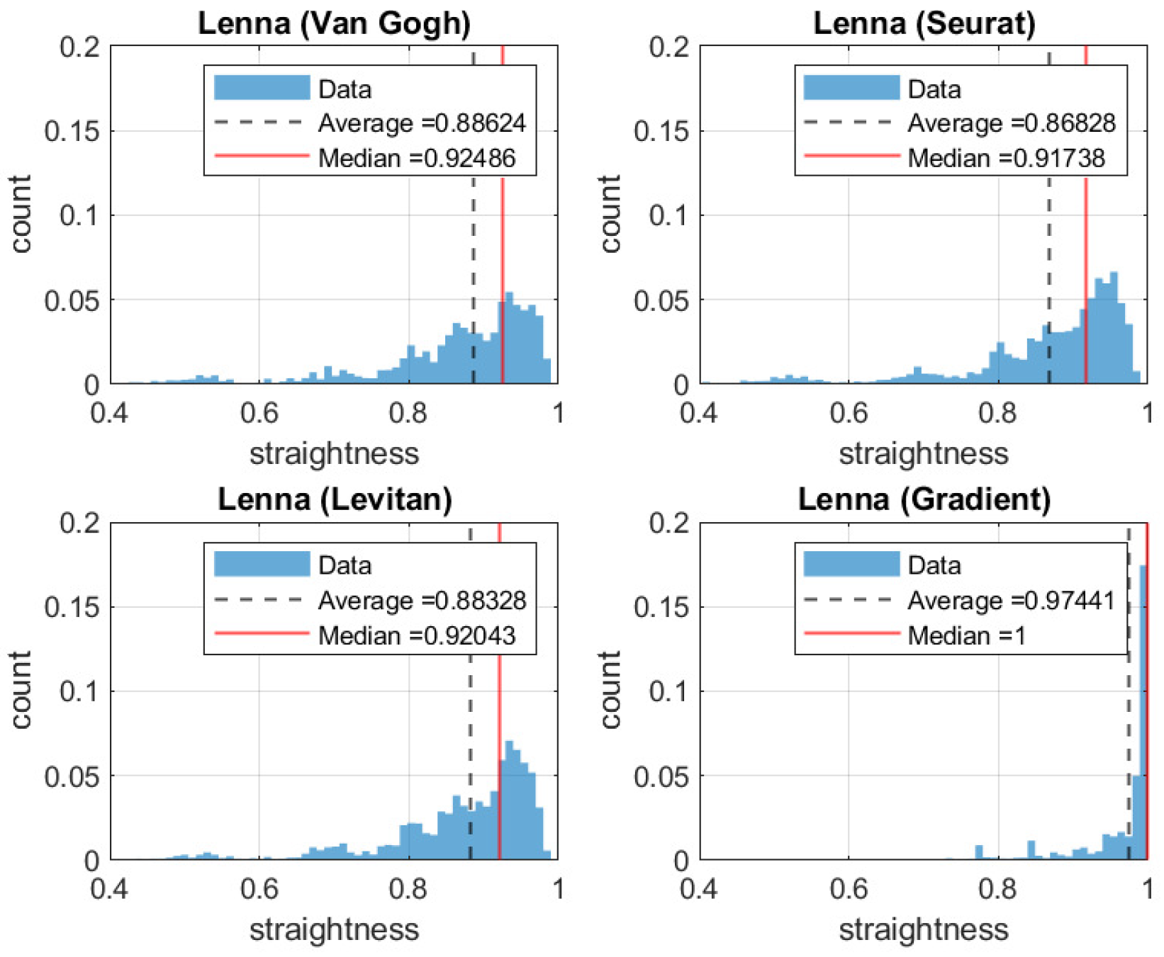
- Straightness. Brushstroke straightness is defined as the Pearson correlation coefficient (PCC) between the horizontal and vertical coordinates of pixels located on the brushstroke skeleton. If the skeleton is a perfectly straight line, the correlation coefficient will be equal to one; if the skeleton is curved, the absolute value of the coefficient will be less than one. Suppose the brushstroke contains N pixels, with coordinates , , , the straightness is defined as:
- Orientation. To obtain the brushstroke orientation, we use an alternative to the definition in [48]. For each brushstroke with , coordinates set, a linear least squares fit is found using the polyfit function in MATLAB. The brushstroke orientation is defined as the slope of the approximating linear polynomial, i.e., as , where k is the first coefficient of the linear polynomial.
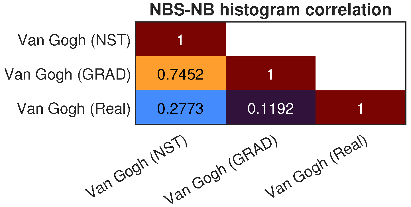
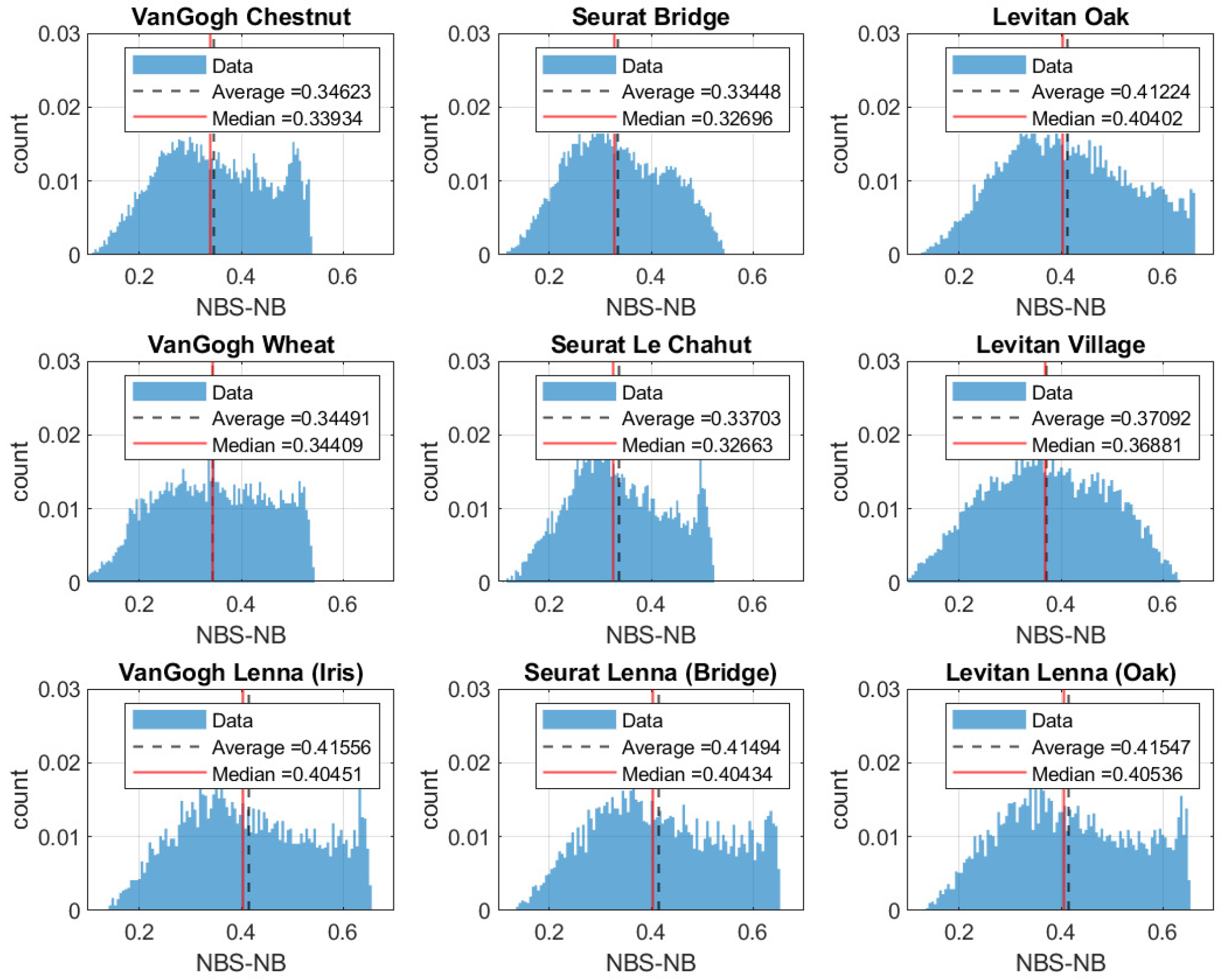
- Number of brushstrokes in the neighborhood (NBS-NB). A brushstroke j is a neighbor to a brushstroke i if the distance between the centers of these brushstrokes does not exceed the threshold value s: and , where the threshold value is set to 200, as in [48]. NBS-NB is the total number of strokes that are neighbors of i.
- Number of brushstrokes with similar orientations in the neighborhood (NBS-SO). A brushstroke j has a similar orientation as i if the difference between their orientations is below a threshold value. The threshold value is set to 0.35, as in [48].
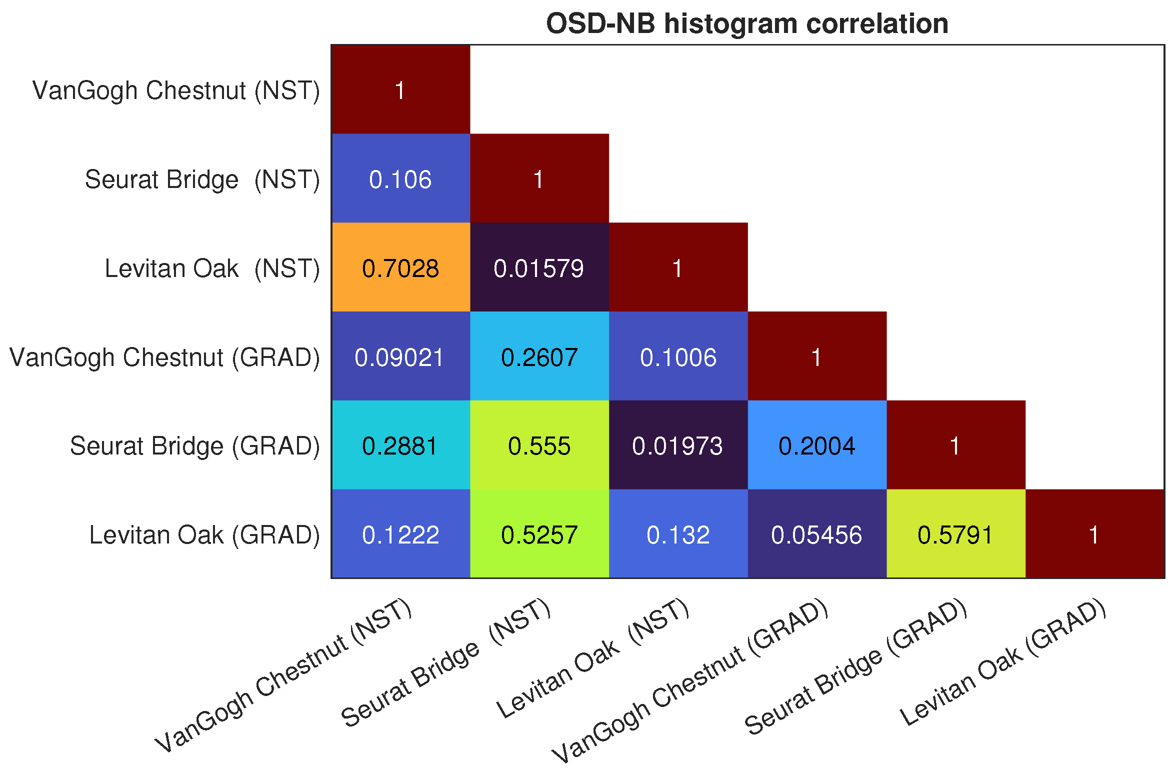
- Orientation standard deviation in the neighborhood (OSD-NB). For any brushstroke i, we compute the orientation standard deviation for all brushstrokes in the neighborhood as:where is the orientation of the i-th stroke in the neighborhood, N is the number of brushstrokes in the neighborhood, and is the mean orientation of all neighboring brushstrokes.
3.4. Test Set
3.5. Design of the Experiment
- Similar artist test. Given nine paintings in three different styles, three artworks in each one, we render them to themselves with the NST algorithm and compare brushstroke parameter distributions. This test aims to learn whether the implementation of the style transfer algorithm from [33] is capable of adapting its results to an individual brushstroke rendering manner.
- NST vs. heuristic test. Given three paintings in different styles, we render them with the NST and heuristic algorithms and compare the brushstroke parameter distributions. This test aims to quantify similarities and differences between the two considered approaches.
- Similar image test. Given one standard image, we render it with the NST program in three different styles and with the heuristic program and then compare brushstroke parameter distributions. This test aims to determine whether differences between these algorithms are substantiated mostly by their design or mostly by the content image.
- Real painting test. Given one image and one parameter which is not radically different in the results given by the two considered algorithms, we compare its distribution with that of the real image investigated in [48]. This test aims to determine which approach gives results closer to the real painting, or whether both are closer to each other than to the real painting.
4. Results
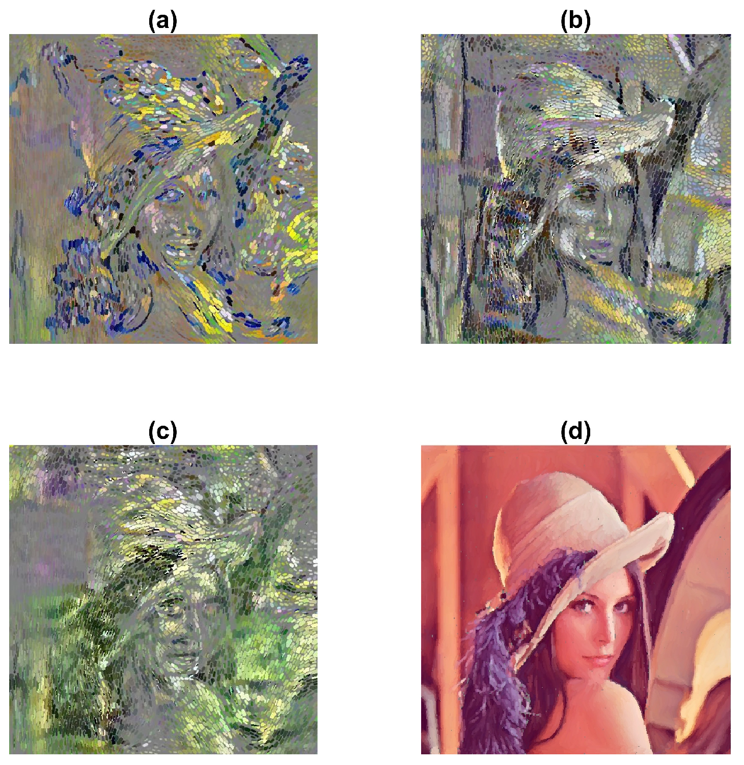
4.1. Examples of Brushstroke Rendering
4.2. Painting-to-Itself by the NST Algorithm Test
4.3. Painting-to-Itself by NST and Gradient Algorithms Test
4.4. Similar Image Test
4.5. Real Painting Test
5. Discussion
6. Conclusions and Future Research
- A novel method for quantifying brushstroke rendering results based on correlation analysis of feature histograms is proposed.
- A comparison of the heuristic gradient-based algorithm with the NST stroke-based algorithm using the proposed method is carried out.
- As a result, the paper offers valuable insights into the limitations of both current style transfer and heuristic techniques and highlights the need for further research to improve their effectiveness.
Author Contributions
Funding
Data Availability Statement
Conflicts of Interest
Abbreviations
| NST | Neural style transfer |
| NBS-NB | Number of neighboring brushstrokes |
| NBS-SO | Number of brushstrokes with similar orientations in the neighborhood |
| OSD-NB | Orientation standard deviation in the neighborhood |
Appendix A. Results for Test 1


Appendix B. Results for Test 2


Appendix C. Results for Test 3


References
- Gooch, B.; Gooch, A. Non-Photorealistic Rendering; CRC Press: Boca Raton, FL, USA, 2001. [Google Scholar]
- Hertzmann, A. Non-photorealistic rendering and the science of art. In Proceedings of the 8th International Symposium on Non-Photorealistic Animation and Rendering, Annecy, France, 7–10 June 2010; pp. 147–157. [Google Scholar]
- Hertzmann, A. Can computers create art? Arts 2018, 7, 18. [Google Scholar] [CrossRef]
- Kumar, M.P.; Poornima, B.; Nagendraswamy, H.; Manjunath, C. A comprehensive survey on non-photorealistic rendering and benchmark developments for image abstraction and stylization. Iran J. Comput. Sci. 2019, 2, 131–165. [Google Scholar] [CrossRef]
- Dijkzeul, D.; Brouwer, N.; Pijning, I.; Koppenhol, L.; Van den Berg, D. Painting with evolutionary algorithms. In Proceedings of the Artificial Intelligence in Music, Sound, Art and Design: 11th International Conference, EvoMUSART 2022, Held as Part of EvoStar 2022, Madrid, Spain, 20–22 April 2022; Springer: Berlin/Heidelberg, Germany, 2022; pp. 52–67. [Google Scholar]
- Scalera, L.; Seriani, S.; Gasparetto, A.; Gallina, P. Non-photorealistic rendering techniques for artistic robotic painting. Robotics 2019, 8, 10. [Google Scholar] [CrossRef]
- Karimov, A.; Kopets, E.; Kolev, G.; Leonov, S.; Scalera, L.; Butusov, D. Image preprocessing for artistic robotic painting. Inventions 2021, 6, 19. [Google Scholar] [CrossRef]
- Karimov, A.I.; Pesterev, D.O.; Ostrovskii, V.Y.; Butusov, D.N.; Kopets, E.E. Brushstroke rendering algorithm for a painting robot. In Proceedings of the 2017 International Conference“ Quality Management, Transport and Information Security, Information Technologies” (IT&QM&IS), Saint Petersburg, Russia, 24–30 September 2017; pp. 331–334. [Google Scholar]
- Gerr, J. The Comic Artist’s Tools Suite: Centralized and Intuitive Non-Photorealistic Computer Graphics Renderings. Ph.D. Thesis, Massachusetts Institute of Technology, Cambridge, MA, USA, 2022. [Google Scholar]
- Mazzone, M.; Elgammal, A. Art, creativity, and the potential of artificial intelligence. Arts 2019, 8, 26. [Google Scholar] [CrossRef]
- Guo, C.; Bai, T.; Lu, Y.; Lin, Y.; Xiong, G.; Wang, X.; Wang, F.Y. Skywork-daVinci: A novel CPSS-based painting support system. In Proceedings of the 2020 IEEE 16th International Conference on Automation Science and Engineering (CASE), Hong Kong, China, 20–21 August 2020; pp. 673–678. [Google Scholar]
- Jing, Y.; Yang, Y.; Feng, Z.; Ye, J.; Yu, Y.; Song, M. Neural style transfer: A review. IEEE Trans. Vis. Comput. Graph. 2019, 26, 3365–3385. [Google Scholar] [CrossRef]
- Singh, A.; Jaiswal, V.; Joshi, G.; Sanjeeve, A.; Gite, S.; Kotecha, K. Neural style transfer: A critical review. IEEE Access 2021, 9, 131583–131613. [Google Scholar] [CrossRef]
- Gatys, L.A.; Ecker, A.S.; Bethge, M. Image style transfer using convolutional neural networks. In Proceedings of the IEEE Conference on computer Vision and Pattern Recognition, Las Vegas, NV, USA, 27–30 June 2016; pp. 2414–2423. [Google Scholar]
- Goodfellow, I.; Pouget-Abadie, J.; Mirza, M.; Xu, B.; Warde-Farley, D.; Ozair, S.; Courville, A.; Bengio, Y. Generative adversarial networks. Commun. ACM 2020, 63, 139–144. [Google Scholar] [CrossRef]
- Cheng, M.M.; Liu, X.C.; Wang, J.; Lu, S.P.; Lai, Y.K.; Rosin, P.L. Structure-preserving neural style transfer. IEEE Trans. Image Process. 2019, 29, 909–920. [Google Scholar] [CrossRef]
- Zhu, J.Y.; Park, T.; Isola, P.; Efros, A.A. Unpaired image-to-image translation using cycle-consistent adversarial networks. In Proceedings of the IEEE International Conference on Computer Vision, Venice, Italy, 22–29 October 2017; pp. 2223–2232. [Google Scholar]
- Isola, P.; Zhu, J.Y.; Zhou, T.; Efros, A.A. Image-to-image translation with conditional adversarial networks. In Proceedings of the IEEE Conference on Computer Vision and Pattern Recognition, Honolulu, HI, USA, 21–26 July 2017; pp. 1125–1134. [Google Scholar]
- Johnson, J.; Alahi, A.; Fei-Fei, L. Perceptual losses for real-time style transfer and super-resolution. In Proceedings of the Computer Vision–ECCV 2016: 14th European Conference, Amsterdam, The Netherlands, 11–14 October 2016; Proceedings, Part II 14. Springer: Berlin/Heidelberg, Germany, 2016; pp. 694–711. [Google Scholar]
- Ulyanov, D.; Lebedev, V.; Vedaldi, A.; Lempitsky, V. Texture networks: Feed-forward synthesis of textures and stylized images. arXiv 2016, arXiv:1603.03417. [Google Scholar]
- Vanderhaeghe, D.; Collomosse, J. Stroke based painterly rendering. In Image and Video-Based Artistic Stylisation; Springer: Berlin/Heidelberg, Germany, 2012; pp. 3–21. [Google Scholar]
- Haeberli, P. Paint by numbers: Abstract image representations. In Proceedings of the 17th Annual Conference on Computer Graphics and Interactive Techniques, Dallas, TX, USA, 6–10 August 1990; pp. 207–214. [Google Scholar]
- Hertzmann, A. Painterly rendering with curved brush strokes of multiple sizes. In Proceedings of the 25th Annual Conference on Computer Graphics and Interactive Techniques, Orlando, FL, USA, 19–24 July 1998; pp. 453–460. [Google Scholar]
- Zeng, K.; Zhao, M.; Xiong, C.; Zhu, S.C. From image parsing to painterly rendering. ACM Trans. Graph. 2009, 29, 2. [Google Scholar]
- Lu, J.; Barnes, C.; DiVerdi, S.; Finkelstein, A. Realbrush: Painting with examples of physical media. ACM Trans. Graph. (TOG) 2013, 32, 1–12. [Google Scholar] [CrossRef]
- Lindemeier, T.; Metzner, J.; Pollak, L.; Deussen, O. Hardware-Based Non-Photorealistic Rendering Using a Painting Robot. Comput. Graph. Forum 2015, 34, 311–323. [Google Scholar] [CrossRef]
- Beltramello, A.; Scalera, L.; Seriani, S.; Gallina, P. Artistic robotic painting using the palette knife technique. Robotics 2020, 9, 15. [Google Scholar] [CrossRef]
- Guo, C.; Bai, T.; Wang, X.; Zhang, X.; Lu, Y.; Dai, X.; Wang, F.Y. ShadowPainter: Active learning enabled robotic painting through visual measurement and reproduction of the artistic creation process. J. Intell. Robot. Syst. 2022, 105, 61. [Google Scholar] [CrossRef]
- Karimov, A.; Kopets, E.; Leonov, S.; Scalera, L.; Butusov, D. A Robot for Artistic Painting in Authentic Colors. J. Intell. Robot. Syst. 2023, 107, 34. [Google Scholar]
- Fu, Y.; Yu, H.; Yeh, C.K.; Lee, T.Y.; Zhang, J.J. Fast accurate and automatic brushstroke extraction. ACM Trans. Multimed. Comput. Commun. Appl. (TOMM) 2021, 17, 1–24. [Google Scholar] [CrossRef]
- Xie, N.; Zhao, T.; Tian, F.; Zhang, X.; Sugiyama, M. Stroke-based stylization learning and rendering with inverse reinforcement learning. In Proceedings of the 24th International Conference on Artificial Intelligence, Buenos Aires, Argentina, 25–31 July 2015; pp. 2531–2537. [Google Scholar]
- Nolte, F.; Melnik, A.; Ritter, H. Stroke-based Rendering: From Heuristics to Deep Learning. arXiv 2022, arXiv:2302.00595. [Google Scholar]
- Kotovenko, D.; Wright, M.; Heimbrecht, A.; Ommer, B. Rethinking style transfer: From pixels to parameterized brushstrokes. In Proceedings of the IEEE/CVF Conference on Computer Vision and Pattern Recognition, Nashville, TN, USA, 20–25 June 2021; pp. 12196–12205. [Google Scholar]
- Mandryk, R.L.; Mould, D.; Li, H. Evaluation of emotional response to non-photorealistic images. In Proceedings of the ACM SIGGRAPH/Eurographics Symposium on Non-Photorealistic Animation and Rendering, Vancouver, BC, Canada, 5–7 August 2011; pp. 7–16. [Google Scholar]
- Mould, D.; Mandryk, R.L.; Li, H. Emotional response and visual attention to non-photorealistic images. Comput. Graph. 2012, 36, 658–672. [Google Scholar] [CrossRef]
- Santella, A.; DeCarlo, D. Visual interest and NPR: An evaluation and manifesto. In Proceedings of the 3rd International Symposium on Non-Photorealistic Animation and Rendering, Annency, France, 7–9 June 2004; pp. 71–150. [Google Scholar]
- Mould, D. Authorial subjective evaluation of non-photorealistic images. In Proceedings of the Workshop on Non-Photorealistic Animation and Rendering, Vancouver, BC, Canada, 8–10 August 2014; pp. 49–56. [Google Scholar]
- Hong, K.; Jeon, S.; Yang, H.; Fu, J.; Byun, H. Domain-aware universal style transfer. In Proceedings of the IEEE/CVF International Conference on Computer Vision, Montreal, BC, Canada, 11–17 October 2021; pp. 14609–14617. [Google Scholar]
- Deng, Y.; Tang, F.; Dong, W.; Ma, C.; Pan, X.; Wang, L.; Xu, C. Stytr2: Image style transfer with transformers. In Proceedings of the IEEE/CVF Conference on Computer Vision and Pattern Recognition, New Orleans, LA, USA, 18–24 June 2022; pp. 11326–11336. [Google Scholar]
- Maciejewski, R.; Isenberg, T.; Andrews, W.M.; Ebert, D.S.; Sousa, M.C.; Chen, W. Measuring stipple aesthetics in hand-drawn and computer-generated images. IEEE Comput. Graph. Appl. 2008, 28, 62–74. [Google Scholar] [CrossRef]
- Dowson, D.; Landau, B. The Fréchet distance between multivariate normal distributions. J. Multivar. Anal. 1982, 12, 450–455. [Google Scholar] [CrossRef]
- Lucic, M.; Kurach, K.; Michalski, M.; Gelly, S.; Bousquet, O. Are gans created equal? A large-scale study. Adv. Neural Inf. Process. Syst. 2018, 31, 698–707. [Google Scholar]
- Wright, M.; Ommer, B. Artfid: Quantitative evaluation of neural style transfer. In Proceedings of the Pattern Recognition: 44th DAGM German Conference, DAGM GCPR 2022, Konstanz, Germany, 27–30 September 2022; Springer: Berlin/Heidelberg, Germany, 2022; pp. 560–576. [Google Scholar]
- Wang, Z.; Zhao, L.; Chen, H.; Zuo, Z.; Li, A.; Xing, W.; Lu, D. Evaluate and improve the quality of neural style transfer. Comput. Vis. Image Underst. 2021, 207, 103203. [Google Scholar] [CrossRef]
- Gatys, L.; Ecker, A.S.; Bethge, M. Texture synthesis using convolutional neural networks. Adv. Neural Inf. Process. Syst. 2015, 28, 262–270. [Google Scholar]
- Karimov, A.I.; Kopets, E.E.; Rybin, V.G.; Leonov, S.V.; Voroshilova, A.I.; Butusov, D.N. Advanced tone rendition technique for a painting robot. Robot. Auton. Syst. 2019, 115, 17–27. [Google Scholar] [CrossRef]
- Lamberti, F.; Sanna, A.; Paravati, G. Computer-assisted analysis of painting brushstrokes: Digital image processing for unsupervised extraction of visible features from van Gogh’s works. EURASIP J. Image Video Process. 2014, 2014, 53. [Google Scholar] [CrossRef]
- Li, J.; Yao, L.; Hendriks, E.; Wang, J.Z. Rhythmic brushstrokes distinguish van Gogh from his contemporaries: Findings via automated brushstroke extraction. IEEE Trans. Pattern Anal. Mach. Intell. 2011, 34, 1159–1176. [Google Scholar]
- Bakurov, I.; Ross, B.J. Non-photorealistic rendering with cartesian genetic programming using graphics processing units. In Proceedings of the Computational Intelligence in Music, Sound, Art and Design: 7th International Conference, EvoMUSART 2018, Parma, Italy, 4–6 April 2018; Springer: Berlin/Heidelberg, Germany, 2018; pp. 34–49. [Google Scholar]
- Collomosse, J.P. Supervised genetic search for parameter selection in painterly rendering. In Proceedings of the Applications of Evolutionary Computing: EvoWorkshops 2006: EvoBIO, EvoCOMNET, EvoHOT, EvoIASP, EvoINTERACTION, EvoMUSART, and EvoSTOC, Budapest, Hungary, 10–12 April 2006; Springer: Berlin/Heidelberg, Germany, 2006; pp. 599–610. [Google Scholar]
- Collomosse, J.P. Evolutionary search for the artistic rendering of photographs. In The Art of Artificial Evolution: A Handbook on Evolutionary Art and Music; Springer: Berlin/Heidelberg, Germany, 2008; pp. 39–62. [Google Scholar]
- Kang, H.W.; Chakraborty, U.K.; Chui, C.K.; He, W. Multi-scale stroke-based rendering by evolutionary algorithm. In Proceedings of the International Workshop on Frontiers of Evolutionary Algorithms, JCIS, Salt Lake City, UT, USA, 21–26 July 2005; pp. 546–549. [Google Scholar]
- Ross, B.J.; Ralph, W.; Zong, H. Evolutionary image synthesis using a model of aesthetics. In Proceedings of the 2006 IEEE International Conference on Evolutionary Computation, Vancouver, BC, Canada, 16–21 July 2006; pp. 1087–1094. [Google Scholar]
- Putri, T.; Mukundan, R.; Neshatian, K. Artistic style characterization and brush stroke modelling for non-photorealistic rendering. In Proceedings of the 2017 International Conference on Image and Vision Computing New Zealand (IVCNZ), Christchurch, New Zealand, 4–6 December 2017; pp. 1–7. [Google Scholar]


| Feature | Images | |
|---|---|---|
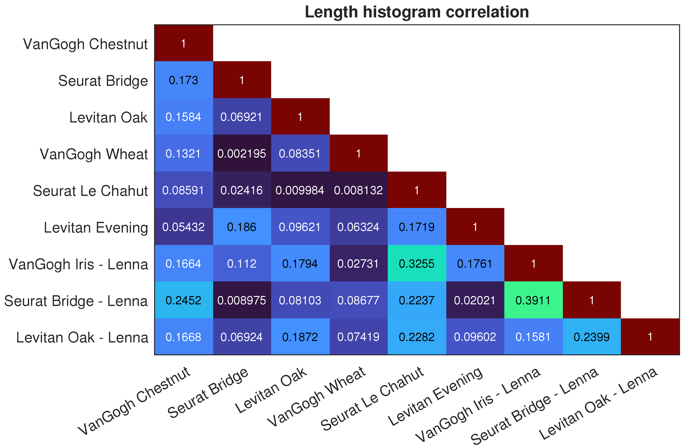
| Length | Seurat Lenna (Bridge), Van Gogh Lenna (Iris) | 0.3911 |
| Seurat Le Chahut, Van Gogh Lenna (Iris) | 0.3255 | |
| Van Gogh Chestnut, Seurat Lenna (Bridge) | 0.2452 | |
| Straightness | Levitan Lenna (Oak), Seurat Lenna (Bridge) | 0.99564 |
| Seurat Le Chahut, Seurat Lenna (Bridge) | 0.98714 | |
| Levitan Lenna (Oak), Seurat Le Chahut | 0.987 | |
| Orientation | Levitan Lenna (Oak), Seurat Lenna (Bridge) | 0.93126 |
| Van Gogh Lenna (Iris), Seurat Lenna (Bridge) | 0.90229 | |
| Van Gogh Chestnut, Seurat Le Chahut | 0.8997 | |
| NBS-NB | Levitan Village, Seurat Bridge | 0.94412 |
| Levitan Lenna (Oak), Seurat Lenna (Bridge) | 0.9184 | |
| Seurat Lenna (Bridge), Levitan Lenna (Oak) | 0.9082 | |
| NBS-SO | Seurat Le Chahut, Seurat Bridge | 0.90952 |
| Levitan Lenna (Oak), Seurat Bridge | 0.86419 | |
| Levitan Oak, Van Gogh Lenna (Iris) | 0.8639 | |
| OSD-NB | Levitan Village, Seurat Le Chahut | 0.83429 |
| Levitan Oak, Van Gogh Chestnut | 0.7028 | |
| Seurat Lenna (Bridge), Van Gogh Lenna (Iris) | 0.6884 |
| Feature | Images | |
|---|---|---|
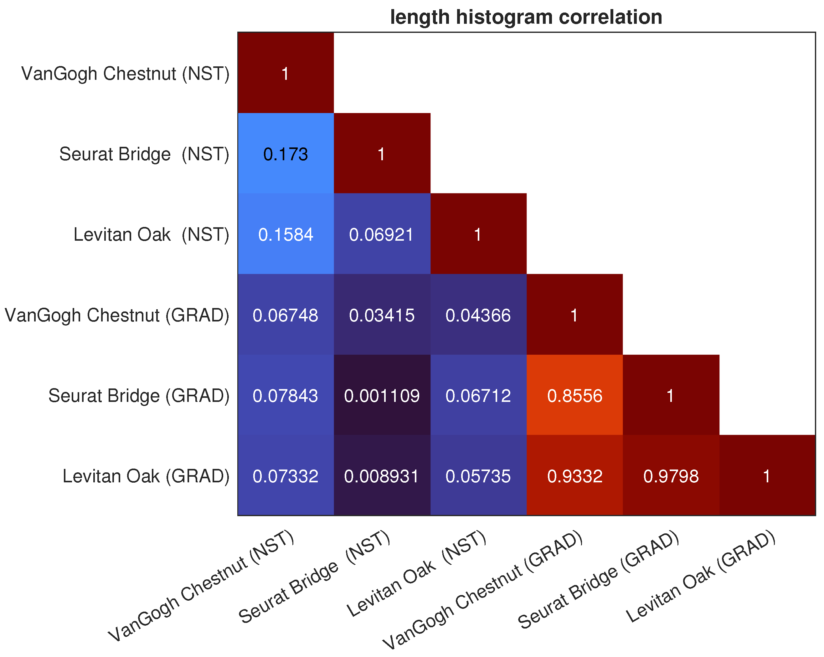
| Length | Levitan Oak (GRAD), Seurat Bridge (GRAD) | 0.97981 |
| Van Gogh Chestnut (GRAD), Levitan Oak (GRAD) | 0.93316 | |
| Seurat Bridge (GRAD), Van Gogh Chestnut (GRAD) | 0.8556 | |
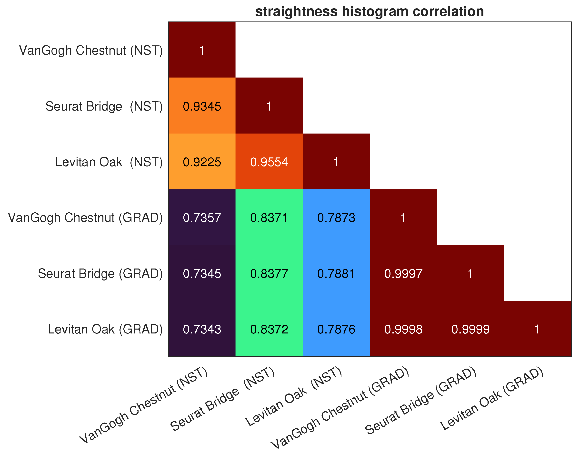
| Straightness | Levitan Oak (GRAD), Seurat Bridge (GRAD) | 0.99993 |
| Van Gogh Chestnut (GRAD), Levitan Oak (GRAD) | 0.99981 | |
| Seurat Bridge (GRAD), Van Gogh Chestnut (GRAD) | 0.9997 | |
| Orientation | Levitan Oak (GRAD), Seurat Bridge (GRAD) | 0.98387 |
| Van Gogh Chestnut (GRAD), Levitan Oak (GRAD) | 0.95169 | |
| Van Gogh Chestnut (GRAD), Seurat Bridge (GRAD) | 0.9377 | |
| NBS-NB | Van Gogh Chestnut (GRAD), Seurat Bridge (NST) | 0.92878 |
| Levitan Oak (NST), Seurat Bridge (NST) | 0.90668 | |
| Van Gogh Chestnut (GRAD), Levitan Oak (NST) | 0.8839 | |
| NBS-SO | Van Gogh Chestnut (GRAD), Van Gogh Chestnut (NST) | 0.8371 |
| Levitan Oak (NST), Van Gogh Chestnut (GRAD) | 0.82775 | |
| Levitan Oak (NST), Seurat Bridge (NST) | 0.82 | |
| OSD-NB | Levitan Oak (NST), Van Gogh Chestnut (NST) | 0.70276 |
| Levitan Oak (GRAD), Seurat Bridge (GRAD) | 0.5791 | |
| Seurat Bridge (NST), Seurat Bridge (GRAD) | 0.55502 |
| Feature | Images | |
|---|---|---|
| Length | Lenna (Seurat), Lenna (Van Gogh) | 0.3911 |
| Lenna (Levitan), Lenna (Seurat) | 0.2399 | |
| Lenna (Van Gogh), Lenna (Seurat) | 0.1856 | |
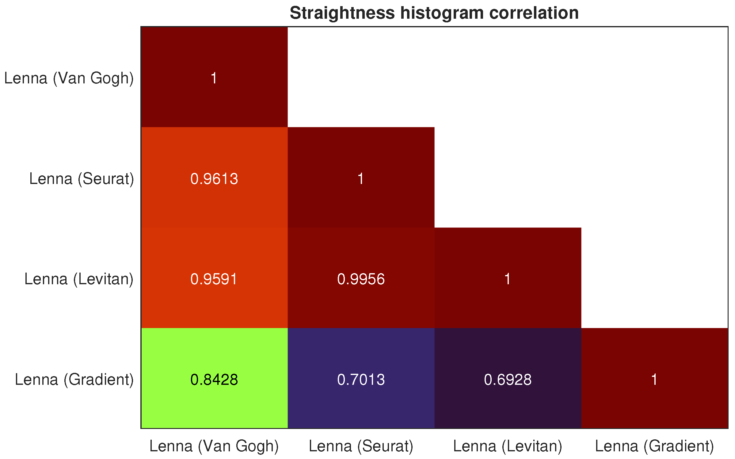
| Straightness | Lenna (Levitan), Lenna (Seurat) | 0.99564 |
| Lenna (Van Gogh), Lenna (Seurat) | 0.96133 | |
| Lenna (Levitan), Lenna (Van Gogh) | 0.9591 | |
| Orientation | Lenna (Levitan), Lenna (Seurat) | 0.93126 |
| Lenna (Van Gogh), Lenna (Seurat) | 0.90229 | |
| Lenna (Levitan), Lenna (Van Gogh) | 0.8639 | |
| NBS-NB | Lenna (Levitan), Lenna (Seurat) | 0.91844 |
| Lenna (Van Gogh), Lenna (Seurat) | 0.90822 | |
| Lenna (Levitan), Lenna (Van Gogh) | 0.898 | |
| NBS-SO | Lenna (Levitan), Lenna (Van Gogh) | 0.84841 |
| Lenna (Seurat), Lenna (Levitan) | 0.83553 | |
| Lenna (Van Gogh), Lenna (Seurat) | 0.8088 | |
| OSD-NB | Lenna (Gradient), Lenna (Seurat) | 0.70927 |
| Lenna (Van Gogh), Lenna (Seurat) | 0.68831 | |
| Lenna (Gradient), Lenna (Van Gogh) | 0.6879 |
Disclaimer/Publisher’s Note: The statements, opinions and data contained in all publications are solely those of the individual author(s) and contributor(s) and not of MDPI and/or the editor(s). MDPI and/or the editor(s) disclaim responsibility for any injury to people or property resulting from any ideas, methods, instructions or products referred to in the content. |
© 2023 by the authors. Licensee MDPI, Basel, Switzerland. This article is an open access article distributed under the terms and conditions of the Creative Commons Attribution (CC BY) license (https://creativecommons.org/licenses/by/4.0/).
Share and Cite
Karimov, A.; Kopets, E.; Shpilevaya, T.; Katser, E.; Leonov, S.; Butusov, D. Comparing Neural Style Transfer and Gradient-Based Algorithms in Brushstroke Rendering Tasks. Mathematics 2023, 11, 2255. https://0-doi-org.brum.beds.ac.uk/10.3390/math11102255
Karimov A, Kopets E, Shpilevaya T, Katser E, Leonov S, Butusov D. Comparing Neural Style Transfer and Gradient-Based Algorithms in Brushstroke Rendering Tasks. Mathematics. 2023; 11(10):2255. https://0-doi-org.brum.beds.ac.uk/10.3390/math11102255
Chicago/Turabian StyleKarimov, Artur, Ekaterina Kopets, Tatiana Shpilevaya, Evgenii Katser, Sergey Leonov, and Denis Butusov. 2023. "Comparing Neural Style Transfer and Gradient-Based Algorithms in Brushstroke Rendering Tasks" Mathematics 11, no. 10: 2255. https://0-doi-org.brum.beds.ac.uk/10.3390/math11102255