Bursting Dynamics in a Singular Vector Field with Codimension Three Triple Zero Bifurcation

Abstract

As a kind of dynamical system with a particular nonlinear structure, a multi-time scale nonlinear system is one of the essential directions of the current development of nonlinear dynamics theory. Multi-time scale nonlinear systems in practical applications are often complex forms of coupling of high-dimensional and high codimension characteristics, leading to various complex bursting oscillation behaviors and bifurcation characteristics in the system. For exploring the complex bursting dynamics caused by high codimension bifurcation, this paper considers the normal form of the vector field with triple zero bifurcation. Two kinds of codimension-2 bifurcation that may lead to complex bursting oscillations are discussed in the two-parameter plane. Based on the fast–slow analysis method, by introducing the slow variable $W=Asin\left(\omega t\right)$, the evolution process of the motion trajectory of the system changing with W was investigated, and the dynamical mechanism of several types of bursting oscillations was revealed. Finally, by varying the frequency of the slow variable, a class of chaotic bursting phenomena caused by the period-doubling cascade is deduced. Developing related work has played a positive role in deeply understanding the nature of various complex bursting phenomena and strengthening the application of basic disciplines such as mechanics and mathematics in engineering practice.

1. Introduction

Multi-time scale nonlinear systems have a broad engineering background. The coupling of different scales involving the interaction of dynamic behavior at multiple scales will lead to many extraordinary nonlinear phenomena. Their complexity and mechanism research has become one of the essential directions for the development of current nonlinear dynamics theory [1]. Most nonlinear systems encountered in natural science and practical engineering applications are coupled by several subsystems [2]. The evolution process from the dynamic behavior at the subsystem level to the dynamic behavior at the fundamental system level will involve different time and space scales, resulting in scale differences between the dynamical characteristics of these subsystems in different environments so that the whole system presents various multi-scale effects [3]. For example, large-scale rotating machinery must consider the large-scale motion of components and the deformation of the members themselves [4], electronic circuit systems with high nonlinear electronic coupling [5,6,7], and the transition metal-catalyzed gas-phase chemical reaction, where adsorption, desorption, and the response between adsorbents are much faster than the oxidation process under the metal surface [8,9]. Such systems cannot be superimposed but exhibit more complex dynamic properties. The process behaves as a typical nonlinear feature, with complex motions such as harmonic oscillations, periodic jumps, quasi-periodic motions, and period-doubling cascades to chaos [10,11]. These nonlinear phenomena can lead to the instability of the entire system in the actual engineering problem, which may be detrimental to industrial applications [12,13]. Therefore, it is urgent to study the dynamic mechanism of such phenomena.

So far, although specific results have been achieved in the complexity of multi-time scale nonlinear systems, due to the particularity of such systems, their related research is still preliminary, and many problems need to be further studied. High codimension bifurcation not only has a variety of bifurcation characteristics but also has a high sensitivity to parameter perturbation, which will not only lead to the diversity of quiescent states and spiking states but, in some circumstances, under the influence of appropriate slow subsystems, it will even lead to the simultaneous existence of different bifurcation characteristics in the same burster. Consequently, in the case of high codimension bifurcation, the fast–slow system has various complex bifurcation characteristics, which leads to the diversification of the motion trajectory of the system. It is necessary to explore the bursting oscillations under high codimension bifurcation and their mechanism.

The qualitative geometry of the flow in each bifurcation form can be obtained by analyzing the dynamic characteristics of the normal form, thereby simplifying the process of analyzing the existing system. Therefore, studying the bursting oscillation behavior of normal form in a singular vector field with high codimension bifurcation has become one of the hot topics [14,15]. The normal form is derived from a simple set of differential equations that study the stability and bifurcation properties of a dynamic system near the equilibria. In addition to the apparent reduction of high-dimensional systems, normal form theory can also classify nonlinear dynamic systems based on the singularity in the unfolding. In recent years, scholars have conducted in-depth research on the complex dynamic behavior of vector fields under high codimension bifurcation. In studying the dynamics of the double pendulum model, Mandadi and Huseyin proposed possible double zero bifurcation, zero-Hopf bifurcation, and double Hopf bifurcation in the system [16]. Yu and Huseyin [17,18] then derived the explicit expression of a singularity normal form with triple zero and zero-zero-Hopf eigenvalues. They explored static and dynamic bifurcation properties of singularity systems near the equilibria, but these results were limited to first-order approximations. Yu and Bi [19] constructed a homogeneous polynomial for calculating the coefficient of normal form using the Lie derivative as an operator for the singular vector field with a Jordan block form in the linear part. They developed the MAPLE program of the corresponding recursive algorithm and studied the dynamic characteristics of a triple zero eigenvalue singularity perturbation model of the double pendulum system on its central manifold. Then, the evolution of the limit cycle near the equilibria of a normal form under the singularity condition is analyzed, and based on that, the complex dynamic behavior, such as chaos induced by the period-doubling cascade, is discussed. Algaba et al. [20,21] discovered similar movements while studying double-zero and triple-zero eigenvalue singularity systems and found a class of global dynamic behavior between homoclinic and heteroclinic orbits. Next, based on the NTT (nonlinear time transformation) method, they derived a recursive algorithm for calculating the analytic formula of the global connection curve of the high-order approximation symmetric Bogdanov–Takens normal form. The theoretically derived phase trajectories can be well matched with the results of numerical simulations [22].

The complex bifurcation characteristics under high codimension bifurcation will lead to the more sophisticated dynamic behavior of fast–slow systems, so scholars at home and abroad have carried out a lot of work studying the mechanism of high codimension bifurcation in the occurrence of complex dynamics of singular systems. Duan et al. [23] classified the burster pattern of the Chay neuron model and divided the bifurcation region within the parametric plane to reveal the dynamical mechanism of bursting oscillations. Next, based on a two-parameter bifurcation analysis, they also found that the codimension-1 and codimension-2 bifurcations of the fast subsystem are essential for the transition mechanisms between different firing activities. The bifurcation curves of the fast subsystem can provide crucial information about the possible types of bursting in the neuronal model under given parameter conditions [24]. Braun and Mereu [25] analyze the zero-Hopf bifurcation occurring in a 3D jerk system after persuading a quadratic perturbation of the coefficients. The second-order averaging theory proves that up to three periodic orbits are born as the perturbation parameter tends to zero. Bao et al. [26] presented a new 5D two-memristor-based jerk (TMJ) system and emphatically studied complex dynamical effects induced by the initial conditions of memristors and non-memristors therein. Consequently, the dynamical effects of the initial conditions on the 5D TMJ system are disclosed comprehensively. Golubitsky et al. [1] proposed a classification method of bursting oscillation, which defined the codimension as the smallest codimension of the first occurrence of singularity in the unfolding by changing the slow-varying unfolding parameter and systematically classifying the currently known busting oscillators induced by the bifurcation of codimension-1 and codimension-2. Saggio [27] conducted a similar study, and they comprehensively classified the burster mode of the fast two-dimensional subsystem on the spherical surface of the unfolding parameter.

This paper studies the bursting oscillation near the codimension-3 triple-zero bifurcation point in the normal form of a singular vector with low-frequency excitation. The rest of this paper is organized as follows: In Section 2, the specific version of the second-order truncated normal form with triple zero eigenvalues singularity in the case of universal folding is introduced. In Section 3, we consider the stabilities and bifurcations of the system by regarding $W=Asin\left(\omega t\right)$ as the bifurcation parameter. In Section 4, the evolution of system dynamics with the change of $W=Asin\left(\omega t\right)$ is analyzed by regarding W as a slow-varying parameter, and the dynamical mechanism of bursting oscillations is investigated by overlapping the transformed phase portrait and the equilibrium branch. Section 5 discusses the chaos evolution caused by the period-doubling cascade. Finally, Section 6 concludes the paper.

2. Mathematical Model

The normal form theory of vector fields provides an effective analytical method for the in-depth study of the stability and bifurcation of high-dimensional nonlinear systems. In addition to the apparent reduction of high-dimensional systems, normal form theory can classify nonlinear dynamic systems according to the singularity in the unfolding. To reveal the complex dynamics of high codimension systems under the effects of fast–slow coupling, this paper analyzes the normal form of a singular vector field with triple zero eigenvalues, the basic idea of which follows.

Consider the following general ODE (ordinary differential equation) system

$$\dot{\mathbf{x}}=\mathbf{Lx}+\mathbf{f}\left(\mathbf{x}\right),\mathbf{f}\in C^k\left(R^n\right),$$

(1)

where $\mathbf{x}\in R^n$ and k is a large number. Without losing the generality, let $\mathbf{x}=0$ be the equilibrium point of the system, namely $\mathbf{f}\left(\mathbf{0}\right)=\mathbf{0}$.

Suppose that the Jordan form of the Jacobian matrix of the system (1) at the equilibrium point is non-semisimple, i.e., it can be expressed as the following block matrix

$$\mathbf{L}=\left[\begin{array}{cc}{\mathbf{L}}_0& 0\\ 0& {\mathbf{L}}_1\end{array}\right]=\left[\begin{array}{cccc}0& 1& 0& 0\\ 0& 0& 1& 0\\ 0& 0& 0& 0\\ 0& 0& 0& {\mathbf{L}}_1\end{array}\right],$$

(2)

where ${\mathbf{L}}_1$ has eigenvalues with nonzero real parts, which are given in Jordan canonical form.

Considering the normal form of the singular vector field under high codimension bifurcation, the calculation of the normal form is complicated because the basis of the corresponding nonlinear transformation is coupled during the calculation process. For a system with the singularity of non-semisimple double zero eigenvalues, Kuznetsov YA [28] analyzed the bifurcation characteristics of its critical normal form in detail. The results have been extended to the study of global bifurcation and chaos [29,30,31,32]. Based on that, Baider and Sanders [33] give a complete formal classification of such systems. For the normal form with the singularity of non-semisimple triple zero eigenvalues, this paper refers to the calculation process proposed by Bi QS and Yu P [19] and introduces a nonlinear transformation

$$\mathbf{w}=\mathbf{u}+\sum _{k\ge 2}{P}^k\left(\mathbf{u}\right)=\mathbf{u}+\mathbf{P}\left(\mathbf{u}\right),$$

(3)

where w is a variable on the central manifold, and the form of a homogeneous polynomial constructed by a set of near-identity transformations is

$${\mathbf{D}}_{\mathbf{u}}\overline{\mathbf{H}}\left(\mathbf{u}\right){\mathbf{L}}_0\mathbf{u}-\mathbf{L}\overline{\mathbf{H}}\left(\mathbf{u}\right)=\mathbf{f}\left(\mathbf{u}\right)-{\mathbf{D}}_{\mathbf{u}}\overline{\mathbf{H}}\left(\mathbf{u}\right)\mathbf{C}\left(\mathbf{u}\right)-\overline{\mathbf{C}}\left(\mathbf{u}\right),$$

(4)

calculating Equation (4) can explicitly express the singularity vector field and its corresponding nonlinear transformation.

When the Jacobian matrix of system (1) has a zero real part of a non-semisimple, i.e., $L_0$ is a non-semisimple form, then $L_0$ can be decomposed into

$${\mathbf{L}}_0=\mathbf{S}+\mathbf{N},$$

(5)

where $\mathbf{S}=diag({\lambda }_1,{\lambda }_2,\dots ,\lambda n_0)$, and $\mathbf{N}$ has the form

$${\mathbf{N}}_{ij}=\left\{\begin{array}{c}1\mathrm{or}0,\mathrm{if}i+1=j;\\ 0,otherwise.\end{array}\right.$$

(6)

By sorting out the coefficients of the nonlinear term ${u_1}^{m_1}{u_2}^{m_2}\dots {u_{n_0}}^{m_{n_0}}$, Equation (6) can be rewritten as

$$({\lambda }_0\mathbf{I}-\mathbf{L}){\mathbf{H}}_{\tilde{m}}+\sum _{j=1}^{n_0-1}{\left({\mathbf{L}}_0\right)}_{j(j+1)}(m_j+1){\mathbf{H}}_{m_1{m}_2\dots (m_{j+1}-1)\dots \left(m_{n_0}\right)}={\tilde{\mathbf{f}}}_{\tilde{m}}-{\overline{\mathbf{C}}}_{\tilde{m}},$$

(7)

Equation (7) can be used to construct algebraic equations which decide the coefficients of normal form with the singularity of triple zero eigenvalues. Then, by performing a series of recursive operations, the explicit expression of the normal form will finally be obtained as

$$\begin{array}{c}{\dot{u}}_1=u_2,\hfill \\ {\dot{u}}_2=u_3,\hfill \\ {\dot{u}}_3={\displaystyle \sum _{j\ge 2}^{\infty }}\begin{array}{c}(C_{3,00(j-1)}{u_3}^{j-1}+({\displaystyle \sum _{l<j}^j}{C}_{3,(j-i)0i}{u_1}^{(j-l)}{u_3}^l\hfill \\ +{\displaystyle \sum _{l<(j-1)}^j}(C_{3,(j-l-1)1i}{u_1}^{j-l-1}{u}_2{u_3}^l+C_{3,(j-l-2)2i}{u_1}^{j-l-2}{u_2}^2{u_3}^l)\left)\right)\hfill \end{array},\hfill \end{array}$$

(8)

where $j=0,1,2,\dots$.

Executing the recursive procedure with MAPLE yields the normal form of a singular vector field truncated to the second order as

$$\begin{array}{c}{\dot{u}}_1=u_2,\hfill \\ {\dot{u}}_2=u_3,\hfill \\ {\dot{u}}_3=C_{3200}{u_1}^2+C_{3020}{u_2}^2+C_{3101}{u}_1{u}_3,\hfill \end{array}$$

(9)

where $C_{i,jkl}$ are the coefficients of normal form.

Inspired by Murdock’s classical unfolding theory [34], the parameter perturbations on constant and linear terms are introduced. Then, the first-order perturbation form of a singular vector field with triple zero eigenvalues is obtained as

$$\dot{\mathbf{w}}=\mathbf{Jw}+\mathbf{F}\left(\mathbf{w}\right)+{\mathbf{Q}}_0\epsilon +{\epsilon }^{\mathrm{T}}{\mathbf{Q}}_1\mathbf{w},$$

(10)

where $\epsilon ={({\epsilon }_1,{\epsilon }_2,{\epsilon }_3)}^T$. $\mathbf{F}\left(\mathbf{w}\right)$ is the vector of nonlinear terms in the canonical form and

$${\mathbf{Q}}_0=\left[\begin{array}{ccc}0& 0& 0\\ 0& 0& 0\\ 1& 0& 0\end{array}\right],{\mathbf{Q}}_1=\left[\begin{array}{ccc}0& 0& 0\\ 0& 1& 0\\ 0& 0& 1\end{array}\right],$$

(11)

then Equation (9) can be rewritten as

$$\begin{array}{c}\dot{x}=y,\hfill \\ \dot{y}=z,\hfill \\ \dot{z}={\epsilon }_1+{\epsilon }_{2}y+{\epsilon }_{3}z+C_{3200}{x}^2+C_{3020}{y}^2+C_{3101}xz.\hfill \end{array}$$

(12)

Introducing a parametric excitation to the system (12), the following non-autonomous singular vector field is established as

$$\begin{array}{c}\dot{x}=y,\hfill \\ \dot{y}=z,\hfill \\ \dot{z}={\mu }_0+({\mu }_1+W)x+{\mu }_{2}y+{\mu }_{3}z+\alpha x^2+\beta y^2+\gamma xz,\hfill \\ W=Asin\left(\omega t\right),\hfill \end{array}$$

(13)

where $\omega \ll 1$, and the parametric excitation W can be expressed as

$$\begin{array}{c}\left\{\begin{array}{c}\dot{W}=\omega W_1,\hfill \\ {\dot{W}}_1=-\omega W,\hfill \end{array}\right.\hfill \end{array}$$

(14)

where $W\left(0\right)=0$, $W_1\left(0\right)=A$.

The system (13) can be treated as a fast–slow system, and W represents the slow variable. Thus, according to the fast–slow analysis method [35], regarding W as a control parameter, the bursting dynamics, especially the transition mechanisms, can be explored.

3. Bifurcation Analyses

Based on the fast–slow analysis method, the system (13) includes fast subsystems that regard W as a control parameter. It can be seen that the equilibrium point of the fast subsystem is in the form $x_E=(\pm x_0,0,0)$, and its solution equation is

$${\mu }_0+({\mu }_1+W)x_E+\alpha {x_E}^2=0,$$

(15)

and the characteristic equation at the equilibrium point is

$$P={\lambda }^3+D_1{\lambda }^2+D_2\lambda +D_3,$$

(16)

where $D_1=-\gamma x_E-{\mu }_1$, $D_2=-{\mu }_1$, and $D_3=-2\alpha x_E-W-{\mu }_1$.

Selecting the system parameter at ${\mu }_1=-0.1,{\mu }_2=-0.16,{\mu }_3=-0.16,\alpha =-0.3,\gamma =-15$. According to the Hurwitz stability criterion, the stability condition of system (14) is $D_3>0$ and $D_1{D}_2-D_3>0$. At this point, the characteristics of the equilibrium point of the system may change through two types of codimension-1 bifurcation. When $D_3=0$, the fold bifurcation may occur, and it will cause the transition between equilibria. The nonhyperbolic condition is

$$\mathrm{fold}:-2\alpha x_{\mathrm{fold}}-W_{\mathrm{fold}}-{\mu }_1=0.$$

(17)

Combining Equations (15) and (17) can obtain bifurcation sets

$$\begin{array}{c}{W_{\mathrm{fold}}}_{+}=0.1+2\sqrt{-0.3{\mu }_0},\hfill \\ {W_{\mathrm{fold}}}_{-}=0.1-2\sqrt{-0.3{\mu }_0},\hfill \end{array}$$

(18)

$W_{{\mathrm{fold}}_{\pm }}$ represents the critical values of W corresponding to the fold bifurcation of the positive and negative half-axis equilibrium point $E_{\pm }$, respectively.

It should be noted that by substituting $W_{{\mathrm{fold}}_{-}}$ and $x_{{\mathrm{fold}}_{-}}$ into Equation (15), the equilibrium of the negative half-axis of x is always unstable, so only the stability of the equilibrium point $E_{+}$ is analyzed below.

When $D_1{D}_2-D_3=0$, the Hopf bifurcation may occur at the equilibrium point. The nonhyperbolic condition is

$$\mathrm{Hopf}:\left(\gamma {\mu }_2+2\alpha \right)x_{\mathrm{Hopf}}+{\mu }_2{\mu }_3+{\mu }_1+W_{\mathrm{Hopf}}=0.$$

(19)

The Hopf bifurcation set can be obtained by solving Equations (15) and (19) simultaneously

$${\mu }_0-0.004645866667+0.1106666667W_{\mathrm{Hopf}}-0.6481481482{W_{\mathrm{Hopf}}}^2=0,$$

(20)

and bursting oscillation occurs when the trajectory on the bifurcation parameters plane crosses it.

When the parameter trajectories meet at the intersection of two codimension-1 bifurcations, fold-Hopf bifurcation may occur, and Hopf bifurcation conditions may also degenerate, resulting in Bautin bifurcation. Here, we use the numerical simulation tool MATCONT to perform codimension-2 bifurcation analysis.

Figure 1 shows a two-parameter bifurcation diagram of the system (13) in the $(W,\beta )$ plane. Due to the previous analysis, only the bifurcation behavior of equilibrium point $E_{+}$ is analyzed here. According to the numerical simulation, it can be obtained that at the point $(-0.13005,7.6881)-(W,\beta )$, the first Lyapunov coefficient $l_1$ shrinks to zero, which means the Hopf bifurcation of $E_{+}$ degenerates, and Bautin bifurcation occurs. Regarding the formula for calculating the second Lyapunov coefficient proposed by Kuznetsov, $l_2=-63.89666<0$ is obtained by numerical simulation. That is, the Bautin bifurcation point $G{H}_{+}=(-0.13005,7.6881)$ in the $(W,\beta )$ plane divides the Hopf bifurcation set $H_{+}$ into two parts: supercritical Hopf bifurcation $(\beta >7.6881)$ and subcritical Hopf bifurcation $(\beta <7.6881)$. To further reveal the mechanism of complex bursting oscillations caused by the codimension-2 Bautin bifurcation, we consider the other dynamics of the system with respect to parameter $W=Asin\left(\omega t\right)$ when $\beta =12$ and $\beta =7.5$, respectively.

3.1. Bifurcation Analysis on $(W,{\mu }_0)$ Plane for $\beta =12$

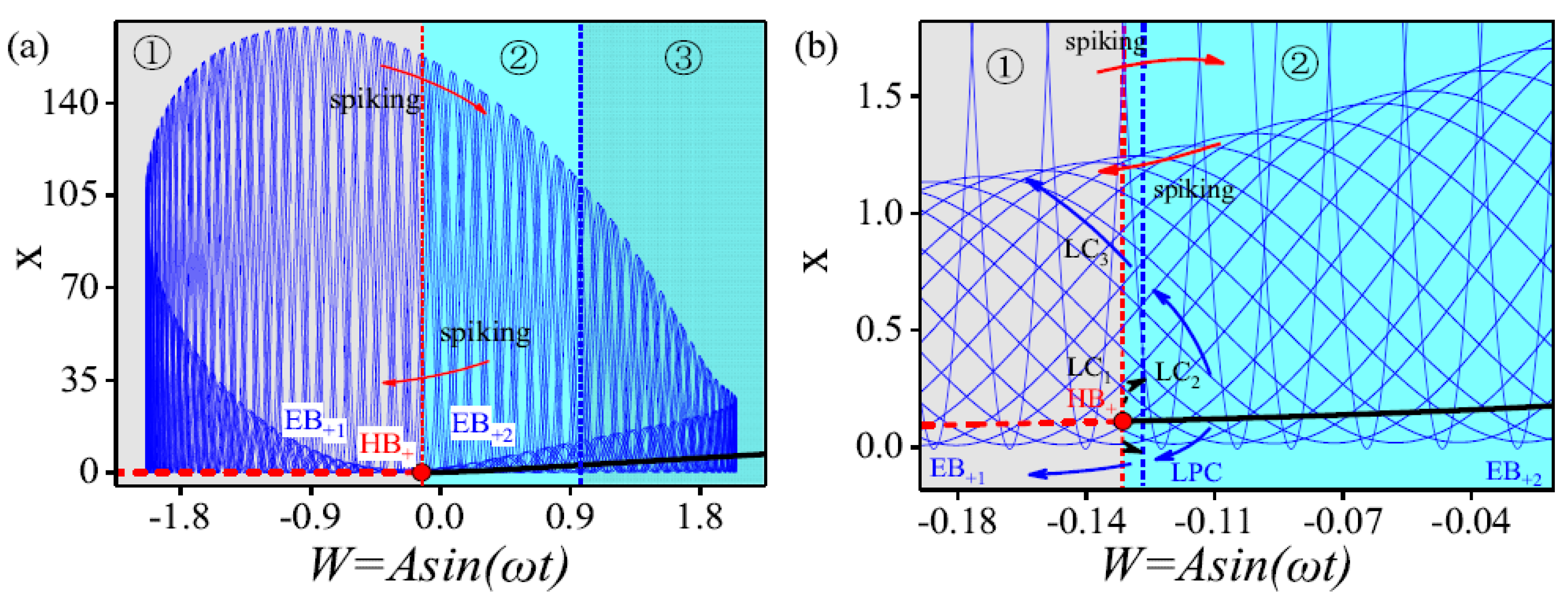
Figure 2 divides the unfolding parameter plane into three regions by the Hopf and fold bifurcation sets. The system dynamics will change accordingly when the unfolding parameter trajectory crosses different areas.

As shown in Figure 2, the system dynamics appear as a stable equilibrium point in region ➁. When the unfolding parameter crosses through the Hopf bifurcation set into region ➀, the supercritical Hopf bifurcation occurs, and the motion trajectory behaves as a stable limit cycle. It should be pointed out that when the parameter changes to $(0.0936,{\tilde{\mu }}_0)-(W,{\mu }_0)$, the bifurcation sets $H_{+}$ and $F_{+}$ intersect at the point $ZH$ where the fold-Hopf bifurcation occurs. Regarding the numerical simulation results, the corresponding fold-Hopf bifurcation coefficients of critical normal form are $s=-1,\sigma =1.5$. In area ➂ of Figure 2, the motion trajectory appears as a stable limit cycle $L{C}_{ZH}$ in the $(x,y)$ plane. Further numerical simulation shows that $L{C}_{ZH}$ will have the period-doubling bifurcation of the limit cycle with the change of slow-varying parameters. Referring to the bifurcation diagram on fold-Hopf bifurcation in the unfolding parametric plane introduced by Kuznetsov, the system will exhibit more rich dynamics when slow-varying parameter W crosses through different regions leading to more complex structures of bursting oscillations.

Figure 3 shows the bifurcation diagram of the system (13) with the variation of slow-varying parameters. The simultaneous Equations (15) and (20) obtain the coordinates $H{B}_{+}=(-0.130049,0.113583)$ of the Hopf bifurcation point of equilibrium point $E_{+}$ in the $(W,x)$ plane. The trajectory behaves as a stable limit cycle $L{C}_{+}$ when the equilibrium branch passes the bifurcation point $H{B}_{+}$. It is worth noting that the numerical simulation results show that $L{C}_{+}$ will bifurcate at $L{C}_{PD}(W=-1.784)$, which will cause the motion trajectory to evolve toward chaos through the period-doubling cascade.

3.2. Bifurcation Analysis on $(W,{\mu }_0)$ Plane for $\beta =7.5$

At $\beta =7.5$, Figure 4 is almost close to Figure 2, but subtle differences remain. Figure 4b shows that a subcritical Hopf bifurcation occurs when the trajectory of W crosses through the Hopf bifurcation set from region ➁ to region ➀. The system behaves as an unstable limit cycle $L{C}_1$. According to the previous analysis, due to the first Lyapunov coefficient failure, the Bautin bifurcation will occur at point $G{H}_{+}$, resulting in a stable limit cycle $L{C}_2$, at which time the second Lyapunov coefficient is $l_2<0$. During the movement of trajectory, $L{C}_1$ and $L{C}_2$ disappear after colliding at $LP{C}_{+}$ $(W=-0.1295)$, creating a new stable limit cycle $L{C}_3$. This process is called FLC (fold bifurcation of the limit cycle).

Figure 5 also shows the bifurcation diagram of the system (13) when ${\mu }_0=0.03$. The coordinates of the Hopf bifurcation point are $H{B}_{+}=(-0.130049,0.113583)$. It can be seen that the fold bifurcation of the limit cycle will cause the structure of the spiking state of the burster to be utterly different from that in the case of $\beta =12$.

4. Evolution of Bursting Oscillations as Well as Their Mechanism

Based on the results of the above analysis, this section will further explore the influence of bifurcation behavior in different regions on the fast–slow effect of the system (13). Here, we also consider the evolution of dynamics in the case of $\beta =12$ and $\beta =7.5$ with the change of the amplitude of the slow-varying parameter W, respectively.

In Figure 6, as the control parameters $W=Asin\left(\omega t\right)$ change, the vertical axis is divided into three areas: red, green, and blue, corresponding to different access modes. Considering the excitation frequency $\omega \ll 1$, the equilibrium branch will slowly cross the corresponding region differently with the excitation amplitude A change, showing various dynamic characteristics.

When $A<\left|W_{ZH}\right|$, the slow-varying excitation $W=Asin\left(\omega t\right)$ will periodically visit the blue area in Figure 6, where the motion trajectory is presented as a stable focus, and no bursting oscillation occurs.

When $A>\left|W_{ZH}\right|$, the red line in Figure 6 represents the curve of W for $A=0.1$, and it can be seen that the control parameter W will visit the blue and green regions over time. Since the bifurcation sets $H_{+}$ and $F_{+}$ intersect at a point in the green area, the codimension-2 fold-Hopf bifurcation will occur. With the perturbance of the high-order term of the system, the trajectory near the equilibria will periodically cross the fold-Hopf bifurcation point, resulting in the motion trajectory near the equilibria appearing as a limit cycle in the $(x,y)$ plane and a stable focus in the $(y,z)$ plane, respectively. The phase portraits of the motion trajectory in different planes and the corresponding time history are performed in Figure 7. In this case, no bursting oscillation occurs.

When $A>\left|W_{Hopf}\right|$, the blue line in Figure 6 represents the curve of slow-varying excitation for $A=0.3$, at which time the control parameters will visit the blue, green, and red regions periodically so that the system dynamics behavior is affected by three areas and bursting oscillations will occur at the single equilibrium point $E_{+}$.

Here, the TPP (transformed phase portrait) is used to reveal the dynamical mechanism of the bursting oscillation behavior of the system. TPP can be defined as

$$\prod _G=[\mathbf{X}\left(\mathbf{t}\right),W]=\left[x\right(t),y(t),z(t),Asin(\omega t\left)\right],\forall t=R$$

(21)

Equation (21) yields the trajectory of the slow-changing parameters associated with each variable of the system (13) in each subplane projection, such as $(W,x)-plane$, $(W,y)-plane$, and $(W,z)-plane$. Therefore, the TPP is believed to present the evolution process of bursting oscillation and reveals the corresponding induction mechanism. Furthermore, here, we overlap the TPP and the equilibrium branch on the $(W,x)-plane$ to demonstrate the characteristics of the equilibrium point and its bifurcation mechanism when bursting oscillation occurs.

4.1. Bursting Oscillation for $\beta =7.5$ as Well as the Mechanism

Let $A=0.3$, and as the slow-variable parameter W changes, the movement trajectory will periodically visit the blue, green, and red regions in Figure 6a. Combined with the bifurcation diagram shown in Figure 4 in the previous section, we can find that in the region ➀, the equilibrium branch of the system will cross the Hopf bifurcation point with the change of W, at which point the trajectory behaves as an unstable limit cycle $L{C}_1$. As the parameters change, the Hopf bifurcation will degenerate, and a stable limit cycle $L{C}_2$ will be generated at the degenerate Hopf bifurcation point $G{H}_{+}$. In Figure 6a, when $W>\left|W_{LPC}\right|$, as W changes further, the two limit cycles will collide, and the limit cycle will bifurcate at position $LPC$, resulting in a stable limit cycle $L{C}_3$.

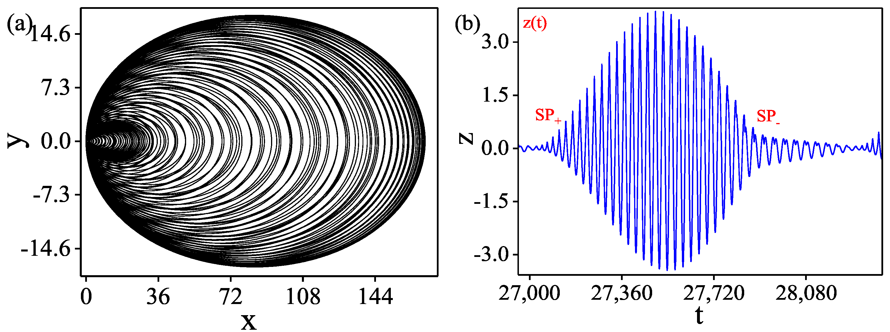
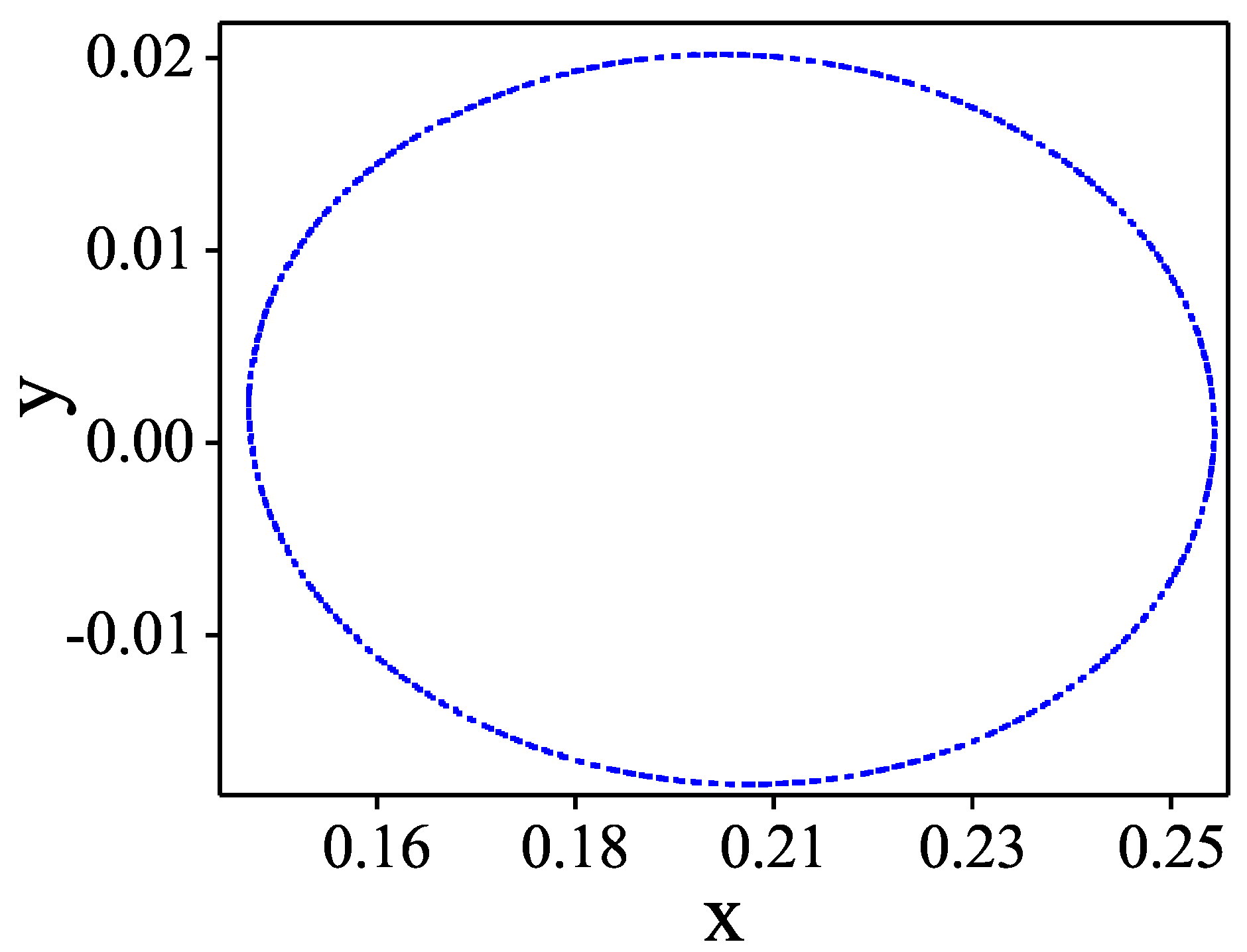
As can be seen from Figure 8, the fast–slow effect occurs between the limit cycle generated by the bifurcation of Hopf and the fold-Hopf bifurcation, resulting in bursting oscillations, and each oscillation period can be divided into the spiking state and the quiescent state. To reveal the essential characteristics of the spiking state, here, the Stroboscopic method is used to obtain the trajectory of the Poincar$\acute{e}$ mapping

$$\sum =[(x,y,z)\left|t=t_0+2N\pi /\omega ,\right.N=1,2,\dots ].$$

(22)

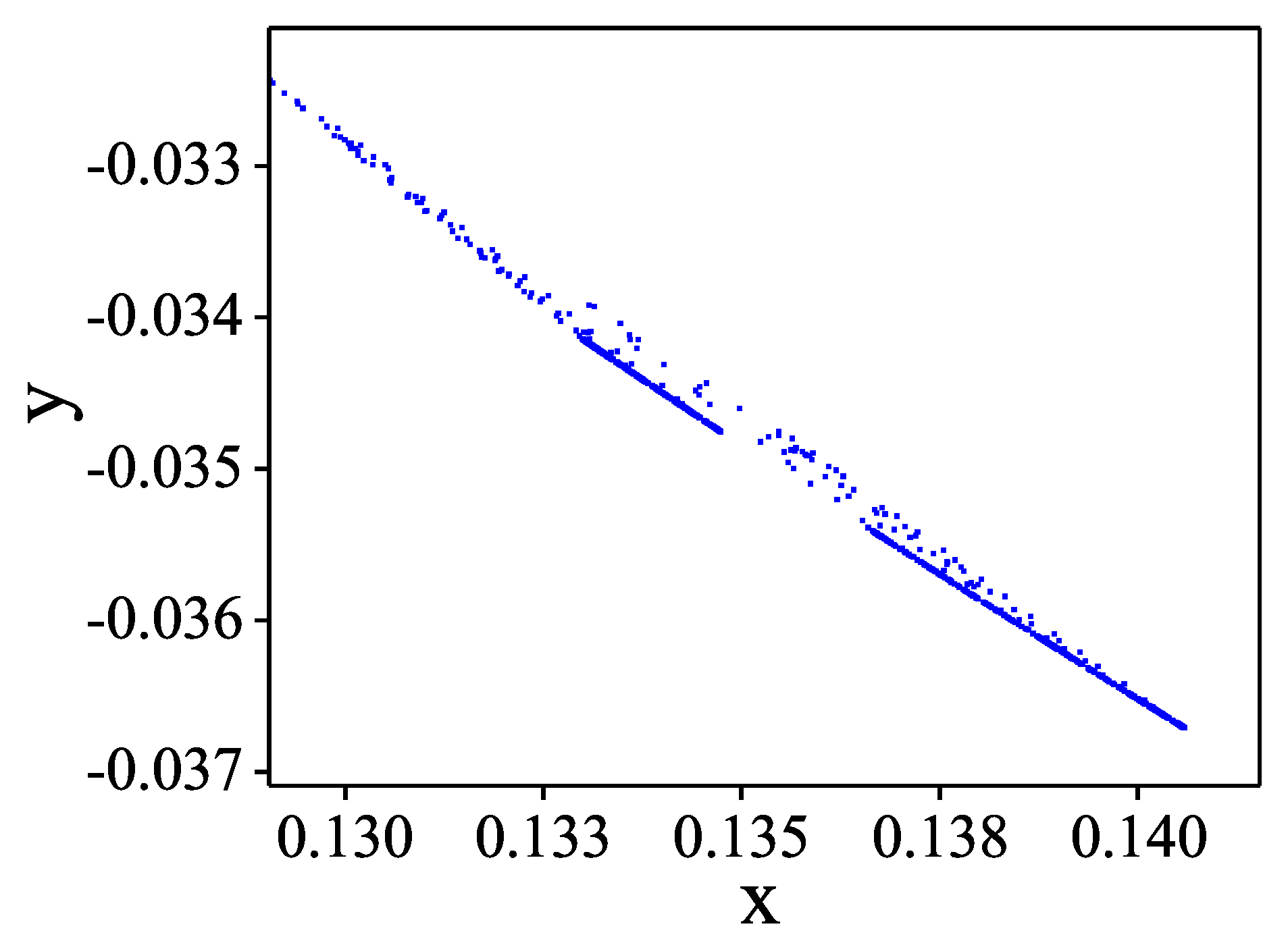
Figure 9 shows the cross-section of the motion trajectory for one period, and it can be found that the spiking state behaves as a quasi-periodic characteristic. Further numerical calculations show that the corresponding two oscillation frequencies approximate the frequency of the stable limit cycle generated by the subcritical Hopf in the red region and the frequency of the limit cycle caused by the fold-Hopf bifurcation in the green area. Therefore, from the structural point of view of bursting oscillation, the burster can be classified as a quasi-periodic Point–Cycle–Cycle type.

As performed in Figure 10, overlapping the TPP and the equilibrium branch in the $(W,x)$ plane, the dynamical mechanism of bursting oscillation can be revealed. Suppose that the motion of the system (13) starts from region ➁, and the trajectory moves to the left along the stable equilibrium branch $E{B}_{+2}$, which appears as a quiescent state. When the trajectory moves to the subcritical Hopf bifurcation point at $H{B}_{+}$, the trajectory will cross this bifurcation point and move along $E{B}_{+1}$ for a while, which is due to the fact that the slow passage effect affects the bifurcation. Some studies in the literature believe that this is in terms of the action of motion inertia, which is affected by factors such as initial value, excitation frequency, and amplitude, which are not discussed here. The effect of Hopf bifurcation occurs after the trajectory passes through the bifurcation delay region in Figure 10, causing the trajectory to jump to the unstable limit cycle $L{C}_1$ and move to the right. When W changes to $W=W_{LPC}$, FLC will occur, causing the unstable limit cycle $L{C}_1$ to disappear after colliding with the stable limit cycle $L{C}_2$ and, at the same time, generating a stable limit cycle $L{C}_3$ in the direction of the left, and the motion trajectory will oscillate according to the stable limit cycle $L{C}_3$, showing a spiking state. When the slow-varying parameter W changes to the minimum value at $W=-0.3$, the trajectory turns, and the slow passage effect of the Hopf bifurcation at point $H{B}_{+}$ makes the amplitude of the trajectory oscillation gradually decreases with the change of W. As W changes, the trajectory will pass through region ➁, enter region ➂, transition to the limit cycle generated by the codimension-2 fold-Hopf bifurcation, and continue oscillating according to the limit cycle, at which point the motion of system still behaves as a spiking state. When the slow-varying parameter W changes to the maximum value $W=0.3$, the trajectory will gradually settle down to the stable equilibrium branch $E{B}_{+2}$ after turning. The trajectory of the system completes a period of bursting oscillations.

In general, the trajectory of bursting oscillation is divided into three parts. Firstly, the trajectory moves along the stable equilibrium branch $E{B}_{+2}$ in region ➁. Secondly, the trajectory oscillates according to the stable limit cycle after passing through the subcritical Hopf bifurcation and FLC in the region ➀. Finally, the trajectory oscillates in the region ➂ by the limit cycle generated by the codimension-2 fold-Hopf bifurcation.

According to the classification method on bursting oscillation proposed by Izhikevich, the oscillation can be called subHopf/FLC/fold-Hopf bursting from the bifurcation mechanism. Meanwhile, from the geometric structure, it can be called a quasi-periodic Point–Cycle–Cycle burster.

The TPP will expand to the left and right as the excitation amplitude increases. Likewise, the trajectory near the equilibria will periodically visit the blue, green, and red regions in Figure 6a. Figure 11 shows the trajectory structure of the system in the $(x,y)$ plane when $A=2.0$ and the corresponding time history. As the slow-varying parameter W changed, the trajectory behaved as a spiking state at all times in the oscillation period. The burster on the spiking state $S{P}_{-}$ presents a period-doubling characteristic. This is caused by the interaction between the limit cycle induced by the fold-Hopf bifurcation of the codimension-2 and the limit cycle generated by the Hopf bifurcation.

Similarly, Figure 12 shows the superposition of the TPP and equilibrium branch in the $(W,x)$ plane when the amplitude of the slow-varying excitation changes to $A=2.0$. It can be seen in the figure that the trajectory of the system motion is almost the same as when $A=0.3$. When the trajectory moves to region ➂ with the change of W, it oscillates according to the limit cycle generated by the fold-Hopf bifurcation, and the system behaves as a spiking state. The trajectory turns and begins to converge toward the stable equilibrium branch $E{B}_{+2}$ when W increases to the maximum value. Before converging to $E{B}_{+2}$, the trajectory moves to a stable limit cycle $L{C}_3$ after it crosses through the Hopf bifurcation point $H{B}_{+}$ and bifurcation delay region, and it oscillates according to the limit cycle $L{C}_3$, at which point the system continues to exhibit a spiking state. This buster can be called a subHopf/FLC/fold-Hopf burster of Cycle–Cycle type.

4.2. Bursting Oscillation for $\beta =12$ as Well as the Mechanism

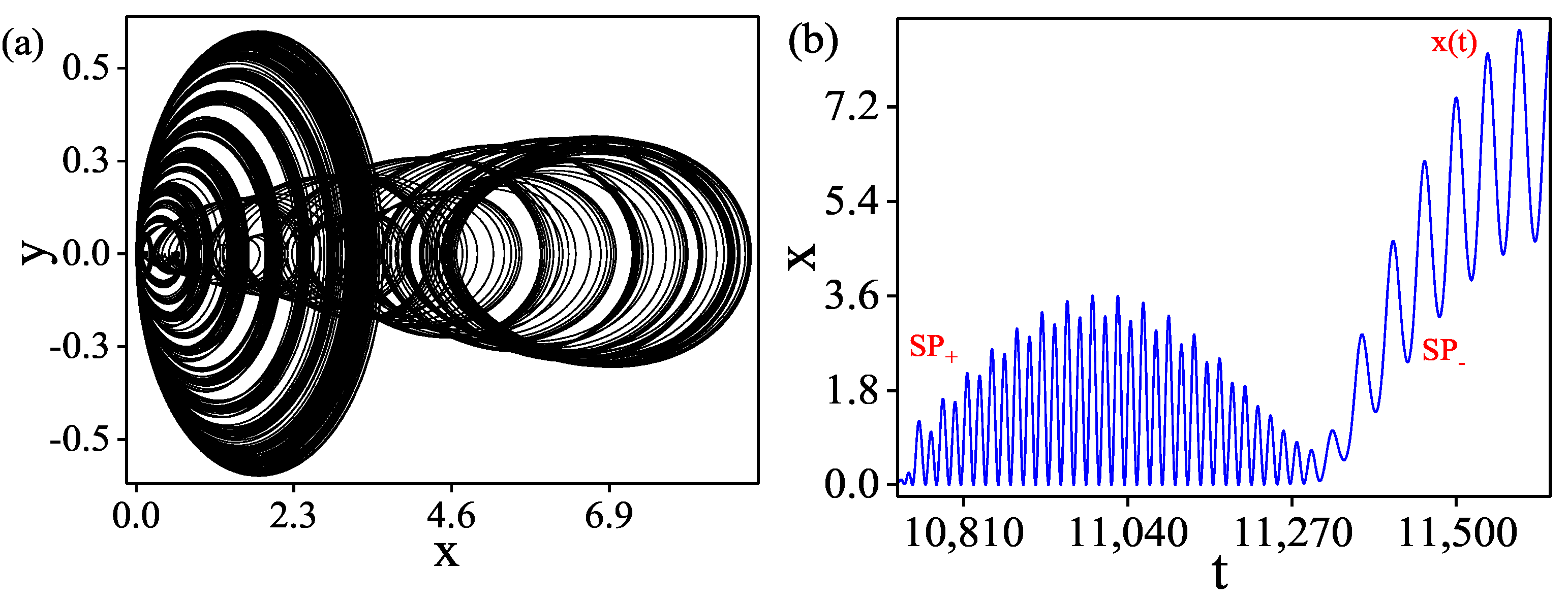
In this case, set $A=0.3$. As shown in Figure 6b, with the changing of the $W=Asin\left(\omega t\right)$, the equilibrium branch of the system will periodically visit regions blue, green, and red sequentially. Figure 13 shows the structure of the trajectory of the system motion in the $(x,y)$ plane and the $(y,z)$ plane, respectively, and the corresponding time history has also been given. It can be seen from Figure 13c,d that when $A=0.3$, with the change of $\beta$, the mode of the spiking state of bursting oscillation due to codimension-2 Bautin bifurcation will change qualitatively, where the red curve represents $\beta =7.5$, and the blue curve represents $\beta =12$.

Figure 14 shows Poincar$\acute{e}$ mapping (22) of the oscillation trajectory of one period, in which it can be found that the spiking state behaves as a quasi-periodic characteristic. Therefore, the structure of the bursting oscillation is the Point–Cycle–Cycle type in this case.

Figure 15 shows the superposition of the TPP and the equilibrium branch on the $(W,x)$ plane. At $A=0.3$, as W changes, the motion trajectory will periodically traverse regions ➁, ➀, and ➂ in Figure 15. Assuming that the starting point of the movement of the system (13) is in region ➁, the trajectory will move to the left along the stable equilibrium branch $E{B}_{+2}$. The system will be quiescent, which can also be confirmed by the $x\left(t\right)$ time history in Figure 13c. By changing W, the supercritical Hopf bifurcation occurs at the bifurcation point $H{B}_{+}$. Due to the delayed effect of the bifurcation, the trajectory will continue to move in the region ➀ along the unstable equilibrium branch $E{B}_{+1}$. When the trajectory crosses the bifurcation delay region in Figure 15b, it will jump to the limit cycle $L{C}_{+}$, causing the trajectory to transition between the spiking state and the quiescent state, and the trajectory will oscillate along $L{C}_{+}$. At the minimum value of W, the trajectory turns the right and oscillates along $L{C}_{+}$. As the slow-varying parameter W changes in the region ➂, the codimension-2 fold-Hopf bifurcation will cause the trajectory to jump toward a stable limit cycle, behaving as a spiking state. When W arrives at the maximum, the trajectory shifts to the left and gradually converges to a stable equilibrium branch, completing one period of bursting oscillation.

The trajectory of bursting oscillation is generally divided into three parts. Firstly, the trajectory moves along the stable equilibrium branch $E{B}_{+1}$ in region ➁. Secondly, it oscillates according to the stable limit cycle after passing through the supercritical Hopf bifurcation in region ➀ and finally oscillates in region ➂ around the limit cycle generated by the codimension-2 fold-Hopf bifurcation.

Due to the interaction between the limit cycle induced by the fold-Hopf bifurcation and the limit cycle generated by the Hopf bifurcation, the spiking state presents a quasi-period characteristic. In this case, the burster can be classified as supHopf/fold-Hopf bursting of Point–Cycle–Cycle type.

As the excitation amplitude A increases, the region the trajectory visits no longer changes. Still, its motion pattern changes, and Figure 16 shows the bursting oscillation when $A=2.0$. From the time history of $x\left(t\right)$ in Figure 16, unlike the case of $A=0.3$, it can be seen that the motion trajectory of the system has been excited at all times. Meanwhile, the trajectory exhibits period-doubling characteristics due to the interaction between the limit cycle generated by the Hopf bifurcation and the limit cycle caused by the fold-Hopf bifurcation. This can also be verified from the time history of the spiking state of bursting oscillation in Figure 16b. The period-doubling characteristic can also be verified by the Poincar$\acute{e}$ mapping of the oscillation trajectory of the burster, which is shown in Figure 17. Consequently, it can be considered that the motion of the system at this time is quasi-period bursting with period-doubling characteristics.

To reveal the mechanism of bursting behavior, as performed in Figure 18, we overlap the TPP and the equilibrium branch. It can be seen that the trajectory of the system motion is almost the same as when $A=0.3$. We assume that the starting point of the trajectory is in region ➁. When the slow-varying parameter W changes to $W=-1.784$, the period-doubling bifurcation of the limit cycle will occur, causing the trajectory to present as Torus. It should be noted that since the inertia of the movement of the system increases with the increase of the excitation amplitude, the trajectory jumps to a stable limit cycle $L{C}_{+}$ before converging to the equilibrium branch and oscillates according to the limit cycle $L{C}_{+}$. At that time, the system continues to exhibit a spiking state. As W changes, the trajectory returns to region ➁, completing one period of bursting oscillation.

5. Evolution of Chaos

This section discusses the evolution of the dynamical behavior when the fast–slow effects change. According to geometric singular perturbation theory, slow manifolds determine the trajectory of the entire fast–slow system, while fast manifolds can be seen as minor perturbations of slow systems. Therefore, in this section, the evolution of the dynamics of the whole system is analyzed by increasing the frequency $\omega$ of the slow variable W. A set of chaotic bursting phenomena induced by the period-doubling cascade of the limit cycle is also deduced.

Let $\beta =12$ and set the excitation amplitude at $A=1.0$. Figure 19 shows the trajectory of bursting oscillation with different $\omega$ values in the $(x,y)$ plane. The corresponding Poincar$\acute{e}$ cross-section is given in Figure 20.

When $\omega =0.005$, from Figure 19a,b, it can be found that the trajectory of the system (13) behaves as a bursting oscillation of a quasi-periodic Cycle–Cycle type. As shown in Figure 19c, when $\omega$ increases to $\omega =0.006$, the trajectory of the bursting presented in the $(x,y)$ plane appears as a doubling period, which is verified by the Poincar$\acute{e}$ mapping of the trajectory corresponding to the bursting oscillation in Figure 19d. Combined with the analysis of Section 3, with the change of unfolding parameters, the limit cycle generated by the codimension-2 fold-Hopf bifurcation evolves to the Torus, resulting in the bursting oscillation present as Torus–Torus type.

As W increases, the trajectory of motion of the system (13) will evolve toward periodic oscillation. Figure 20 shows that the scale difference between the frequency of the spiking state $S{P}_{+}$ and $S{P}_{-}$ of the burster is gradually disappearing. From the time history of $x\left(t\right)$ in Figure 20b,d, the difference in time scale between the two spiking states still exists, so it can be considered that the motion trajectory of the system at this time is a bursting oscillation. Figure 20a,c show that the trajectory of the burster is period-4 for $\omega =0.024$ and period-8 for $\omega =0.026$, respectively. When $\omega$ increases to $\omega =0.037$, the trajectory of bursting in the $(x,y)$ plane appears irregular, which can be verified in Figure 20f. At this point, it can be considered that the motion of the system evolved from the period-doubling cascade to chaotic bursting.

As $\omega$ increases further, the scale differences between the fast and slow subsystems will disappear completely, and Figure 21 also deduces a set of chaotic motions induced by the period-doubling cascade. The corresponding $\omega$ are $\omega =0.109$ (period-2), $\omega =0.111$ (period-4), $\omega =0.112$ (period-8) and $\omega =0.113$ (chaos), respectively.

6. Conculusions

This paper mainly studies the bursting oscillations and their dynamical mechanism of the second-order truncated triple zero eigenvalues singularity normal form under the unfolding form. Based on the fast–slow analysis method, considering the order gap between excitation and natural frequency, the singular system with parametric excitation can be viewed as a generalized autonomous system. The evolution of system dynamics and the mechanism are analyzed regarding periodic parameter excitation $W=Asin\left(\omega t\right)$ as a slow-varying bifurcation parameter. The system exhibits various bursting oscillation patterns when the slow-varying parameters visit different dynamical regions in the two-parameter plane. In particular, due to the singularity of the triple zero eigenvalues, two types of degeneration will occur in the Hopf bifurcation at the equilibrium point of the system, namely the codimension-2 fold-Hopf bifurcation and the Bautin bifurcation, which makes the dynamic behavior change from simple to complex. More diverse structures of the spiking state of bursting oscillation will occur at the single equilibria due to the complexity of the singularity of high codimension bifurcation, such as Cycle–Cycle burster, Torus–Torus burster, and chaotic bursting. With the increase of the approximate order of normal form, the number of equilibrium points of the system will increase, and the difficulty of bifurcation analysis will also increase, so the dynamical mechanism corresponding to bursting oscillations will also become complex, and related research needs to be further carried out.

References

- Golubitsky, M.; Josic, K.; Kaper, T.J. An unfolding theory approach to bursting in fast-slow systems. In Global Analysis of Dynamical Systems, A Festschrift/Liber Amicorum Dedicated to Floris Takens for His 60th Birthday; Broer, H., Krauskopf, B., Vegter, G., Eds.; IOP Publishing: Bristol, UK, 2001; pp. 277–308. [Google Scholar] [CrossRef]
- Leimkuhler, B. An efficient multiple time-scale reversible integrator for the gravitational N-body problem. Appl. Numer. Math. 2002, 43, 175–190. [Google Scholar] [CrossRef]
- Fujimoto, K.; Kaneko, K. How fast elements can affect slow dynamics. Phys. D Nonlinear Phenom. 2003, 180, 1–16. [Google Scholar] [CrossRef]
- Hou, L.; Chen, H.; Chen, Y.; Lu, K.; Liu, Z. Bifurcation and stability analysis of a nonlinear rotor system subjected to constant excitation and rub-impact. Mech. Syst. Signal Process. 2019, 125, 65–78. [Google Scholar] [CrossRef]
- Bonet, C.; Jeffrey, M.R.; Martín, P.; Olm, J.M. Novel slow–fast behaviour in an oscillator driven by a frequency-switching force. Commun. Nonlinear Sci. Numer. Simul. 2023, 118, 107032. [Google Scholar] [CrossRef]
- Bao, H.; Wang, N.; Bao, B.; Chen, M.; Jin, P.; Wang, G. Initial condition-dependent dynamics and transient period in memristor-based hypogenetic jerk system with four line equilibria. Commun. Nonlinear Sci. Numer. Simul. 2018, 57, 264–275. [Google Scholar] [CrossRef]
- Bi, Q.; Li, S.; Kurths, J.; Zhang, Z. The mechanism of bursting oscillations with different codimensional bifurcations and nonlinear structures. Nonlinear Dyn. 2016, 85, 993–1005. [Google Scholar] [CrossRef]
- Györgyi, L.; Field, R.J. A three-variable model of deterministic chaos in the Belousov–Zhabotinsky reaction. Nature 1992, 355, 808–810. [Google Scholar] [CrossRef]
- Vanag, V.K.; Zhabotinsky, A.M.; Epstein, I.R. Oscillatory clusters in the periodically illuminated, spatially extended Belousov-Zhabotinsky reaction. Phys. Rev. Lett. 2001, 86, 552. [Google Scholar] [CrossRef]
- Huang, L.; Wu, G.; Zhang, Z.; Bi, Q. Fast–slow dynamics and bifurcation mechanism in a novel chaotic system. Int. J. Bifurc. Chaos 2019, 29, 1930028. [Google Scholar] [CrossRef]
- Wang, J. Active vibration control: Design towards performance limit. Mech. Syst. Signal Process. 2022, 171, 108926. [Google Scholar] [CrossRef]
- Dragan, V.; Stoica, A. Robust stabilization of two-time scale systems with respect to the normalized coprime factorization. Int. J. Control 2002, 75, 1–10. [Google Scholar] [CrossRef]
- Boussaada, I.; Morărescu, I.-C.; Niculescu, S. Inverted pendulum stabilization: Characterization of codimension-three triple zero bifurcation via multiple delayed proportional gains. Syst. Control Lett. 2015, 82, 1–9. [Google Scholar] [CrossRef]
- Xue, M.; Gou, J.; Xia, Y.; Bi, Q. Computation of the normal form as well as the unfolding of the vector field with zero-zero-Hopf bifurcation at the origin. Math. Comput. Simul. 2021, 190, 377–397. [Google Scholar] [CrossRef]
- Zhang, M.; Zhang, X.; Bi, Q. Slow–Fast Behaviors and Their Mechanism in a Periodically Excited Dynamical System with Double Hopf Bifurcations. Int. J. Bifurc. Chaos 2021, 31, 2130022. [Google Scholar] [CrossRef]
- Mandadi, V.; Huseyin, K. Non-linear bifurcation analysis of non-gradient systems. Int. J. Non-Linear Mech. 1980, 15, 159–172. [Google Scholar] [CrossRef]
- Yu, P.; Huseyin, K. Bifurcations associated with a three-fold zero eigenvalue. Q. Appl. Math. 1988, 46, 193–216. [Google Scholar] [CrossRef]
- Yu, P.; Huseyin, K. Bifurcations associated with a double zero of index two and a pair of purely imaginary eigenvalues. Int. J. Syst. Sci. 1988, 19, 1–21. [Google Scholar] [CrossRef]
- Bi, Q.; Yu, P. Computation of normal forms of differential equations associated with non-semisimple zero eigenvalues. Int. J. Bifurc. Chaos 1998, 8, 2279–2319. [Google Scholar] [CrossRef]
- Freire, E.; Gamero, E.; Rodríguez-Luis, A.J.; Algaba, A. A note on the triple-zero linear degeneracy: Normal forms, dynamical and bifurcation behaviors of an unfolding. Int. J. Bifurc. Chaos 2002, 12, 2799–2820. [Google Scholar] [CrossRef]
- Algaba, A.; Domínguez-Moreno, M.C.; Merino, M.; Rodríguez-Luis, A.J. Takens–Bogdanov bifurcations of equilibria and periodic orbits in the Lorenz system. Commun. Nonlinear Sci. Numer. Simul. 2016, 30, 328–343. [Google Scholar] [CrossRef]
- Algaba, A.; Chung, K.-W.; Qin, B.-W.; Rodríguez-Luis, A.J. Computation of all the coefficients for the global connections in the Z2-symmetric Takens-Bogdanov normal forms. Commun. Nonlinear Sci. Numer. Simul. 2020, 81, 105012. [Google Scholar] [CrossRef]
- Duan, L.; Lu, Q.; Wang, Q. Two-parameter bifurcation analysis of firing activities in the Chay neuronal model. Neurocomputing 2008, 72, 341–351. [Google Scholar] [CrossRef]
- Duan, L.; Lu, Q.; Cheng, D. Bursting of Morris-Lecar neuronal model with current-feedback control. Sci. China Ser. E Technol. Sci. 2009, 52, 771–781. [Google Scholar] [CrossRef]
- Braun, F.; Mereu, A.C. Zero-Hopf bifurcation in a 3D jerk system. Nonlinear Anal. Real World Appl. 2021, 59, 103245. [Google Scholar] [CrossRef]
- Bao, H.; Ding, R.; Hua, M.; Wu, H.; Chen, B. Initial-condition effects on a two-memristor-based Jerk system. Mathematics 2022, 10, 411. [Google Scholar] [CrossRef]
- Saggio, M.L.; Spiegler, A.; Bernard, C.; Jirsa, V.K. Fast–slow bursters in the unfolding of a high codimension singularity and the ultra-slow transitions of classes. J. Math. Neurosci. 2017, 7, 7. [Google Scholar] [CrossRef]
- Kuznetsov, Y.A. Elements of Applied Bifurcation Theory, 2nd ed.; Springer: New York, NY, USA, 2011. [Google Scholar]
- Sen, D.; Ghorai, S.; Banerjee, M.; Morozov, A. Bifurcation analysis of the predator–prey model with the Allee effect in the predator. J. Math. Biol. 2022, 84, 7. [Google Scholar] [CrossRef]
- Yang, R. Turing–Hopf bifurcation co-induced by cross-diffusion and delay in Schnakenberg system. Chaos Solitons Fractals 2022, 164, 112659. [Google Scholar] [CrossRef]
- Maleki, F.; Beheshti, B.; Hajihosseini, A.; Lamooki, G.R.R. The Bogdanov–Takens bifurcation analysis on a three dimensional recurrent neural network. Neurocomputing 2010, 73, 3066–3078. [Google Scholar] [CrossRef]
- Perko, L.M. A global analysis of the Bogdanov–Takens system. SIAM J. Appl. Math. 1992, 52, 1172–1192. [Google Scholar] [CrossRef]
- Baider, A.; Sanders, J.A. Further reduction of the Takens-Bogdanov normal form. J. Differ. Equ. 1992, 99, 205–244. [Google Scholar] [CrossRef]
- Murdock, J. Asymptotic unfoldings of dynamical systems by normalizing beyond the normal form. J. Differ. Equ. 1998, 143, 151–190. [Google Scholar] [CrossRef]
- Rinzel, J. Formal classification of bursting mechanisms in excitable systems. In Lecture Notes in Biomathematics; Teramoto, E., Yamaguti, M., Eds.; Springer: Berlin, Germany, 1987; pp. 267–281. [Google Scholar]
Figure 1.
Two-parameter bifurcation diagram in the () plane.
Figure 2.
Two-parameter bifurcation diagram in the () plane for . (a) The framework of the bifurcation diagram. (b) Local enlargement of the bifurcation diagram.
Figure 3.
Single-parameter bifurcation diagram on the () plane for .
Figure 4.
Two-parameter bifurcation diagram on the () plane for . (a) The framework of the bifurcation diagram. (b) Local enlargement of the bifurcation diagram.
Figure 5.
Figure 6.
The trace path of the equilibrium branch as it changes with W. (a) The case for . (b) The case for .
Figure 7.
The phase portrait of system trajectory and its time history for . (a) The phase portrait on the () plane. (b) The phase portrait on the () plane. (c) The time history of . (d) The time history of .
Figure 8.
The bursting oscillation for . (a) The phase portrait on the plane. (b) The phase portrait on the plane. (c) The time history of . (d) The time history of .
Figure 9.
The trajectory of Poincar mapping corresponding to the bursting oscillations for .
Figure 10.
TPP on the () plane for . (a) The framework of the TPP. (b) Local enlargement of the TPP.
Figure 11.
The bursting oscillation for . (a) The phase portrait on the () plane. (b) The time history of .
Figure 12.
TPP on the plane for . (a) Framework of the TPP. (b) Local enlargement of the TPP.
Figure 13.
The bursting oscillation for . (a) The phase portrait on the () plane. (b) The phase portrait on the () plane. (c) Overlap of the time history of . (d) Overlap of the time history of .
Figure 14.
Poincar mapping (22) for .
Figure 15.
TPP on the for () plane. (a) The framework of the TPP. (b) Local enlargement of the TPP.
Figure 16.
Figure 17.
Figure 18.
TPP for the () plane for . (a) The framework of the TPP. (b) Local enlargement of the TPP.
Figure 19.
Evolution of bursting oscillations with period-doubling. (a) Quasi-period bursting for . (b) Poincar mapping (22) for . (c) Quasi-period bursting for . (d) Poincar mapping (22) for as well as the time history of .
Figure 20.
The evolution of a period-doubling cascade to chaotic bursting. (a) Bursting with period doubling for . (b) Poincar mapping (22) for as well as the time history of . (c) Bursting with period doubling for ; (d) Poincar mapping (22) for as well as the time history of . (e) Chaotic bursting; (f) Poincar mapping (22) for as well as the time history of .
Figure 21.
The evolution of a period-doubling cascade to chaos. (a) PD-2 for . (b) PD-4 for . (c) PD-8 for . (d) Chaos for .
Disclaimer/Publisher’s Note: The statements, opinions and data contained in all publications are solely those of the individual author(s) and contributor(s) and not of MDPI and/or the editor(s). MDPI and/or the editor(s) disclaim responsibility for any injury to people or property resulting from any ideas, methods, instructions or products referred to in the content. |
© 2023 by the authors. Licensee MDPI, Basel, Switzerland. This article is an open access article distributed under the terms and conditions of the Creative Commons Attribution (CC BY) license (https://creativecommons.org/licenses/by/4.0/).
Share and Cite
MDPI and ACS Style
Lyu, W.; Li, S.; Chen, Z.; Bi, Q. Bursting Dynamics in a Singular Vector Field with Codimension Three Triple Zero Bifurcation. Mathematics 2023, 11, 2486. https://0-doi-org.brum.beds.ac.uk/10.3390/math11112486
AMA Style
Lyu W, Li S, Chen Z, Bi Q. Bursting Dynamics in a Singular Vector Field with Codimension Three Triple Zero Bifurcation. Mathematics. 2023; 11(11):2486. https://0-doi-org.brum.beds.ac.uk/10.3390/math11112486
Chicago/Turabian StyleLyu, Weipeng, Shaolong Li, Zhenyang Chen, and Qinsheng Bi. 2023. "Bursting Dynamics in a Singular Vector Field with Codimension Three Triple Zero Bifurcation" Mathematics 11, no. 11: 2486. https://0-doi-org.brum.beds.ac.uk/10.3390/math11112486
Note that from the first issue of 2016, this journal uses article numbers instead of page numbers. See further details here.