Greenhouse Micro-Climate Prediction Based on Fixed Sensor Placements: A Machine Learning Approach

Abstract

Accurate measurement of micro-climates that include temperature and relative humidity is the bedrock of the control and management of plant life in protected cultivation systems. Hence, the use of a large number of sensors distributed within the greenhouse or mobile sensors that can be moved from one location to another has been proposed, which are both capital and labor-intensive. On the contrary, accurate measurement of micro-climates can be achieved through the identification of the optimal number of sensors and their optimal locations, whose measurements are representative of the micro-climate in the entire greenhouse. However, given the number of sensors, their optimal locations are proven to vary from time to time as the outdoor weather conditions change. Therefore, regularly shifting the sensors to their optimal locations with the change in outdoor conditions is cost-intensive and may not be appropriate. In this paper, a framework based on the dense neural network (DNN) is proposed to predict the measurements (temperature and humidity) corresponding to the optimal sensor locations, which vary relative to the outdoor weather, using the measurements from sensors whose locations are fixed. The employed framework demonstrates a very high correlation between the true and predicted values with an average coefficient value of 0.91 and 0.85 for both temperature and humidity, respectively. In other words, through a combination of the optimal number of fixed sensors and DNN architecture that performs multi-channel regression, we estimate the micro-climate of the greenhouse.

1. Introduction

Agricultural products are crucial to the sustenance of humans and livestock. However, their production is faced with several challenges such as extreme weather conditions, soil erosion, pests, and disease outbreaks, which all have far-reaching effects on crop productivity and growth rate [1,2]. Protected cultivation systems such as greenhouses offer optimal production of agricultural products throughout the year by the appropriate control of micro- and macro-environments suitable for plant growth [3]. Furthermore, protected cultivation systems result in higher income compared to open-field cultivation as a result of their higher returns per unit area [4]. Hence, their adoption is increasing across continents [5]. Despite these benefits, the operation of greenhouses is non-linear in nature due to changing atmospheric conditions [6] and therefore requires intricate monitoring and control to obtain optimal yield. In other words, maintaining suitable temperature, which directly affects the humidity, is essential in greenhouse environmental control as these affect crop growth as well as quality and quantity [7,8,9]. Specifically, while effective temperature control improves plant growth and minimizes the energy consumed by the system, an appropriate relative humidity range is required to prevent fungal infection and control transpiration [10].

To facilitate monitoring and control in protected cultivation systems, the integration of different advanced sensing technologies becomes eminent [4,11,12]. Basically, sensors installed in greenhouses range from those used to monitor and control micro-climatic conditions such as temperature and relative humidity to soil-related parameters such as moisture, PH, and several others, which are vital for maintaining optimal conditions for favorable crop productivity and growth. In terms of micro-climates, previous studies have shown that monitoring and controlling the temperature and relative humidity within a greenhouse is complex and challenging due to drastic variations in daily and seasonal atmospheric conditions [13].

Generally, sensors are installed arbitrarily in protected systems based on factors such as grower resources, the size of the facility, and technical know-how [14]. Furthermore, in conventional settings, as many sensors as possible are usually installed to facilitate the necessary measurements. However, the use of multiple randomly/inappropriately placed sensors fails to provide measurements that are true estimates of greenhouse micro-climates. In addition, employing a large number of sensors results in large quantities of data that require efficient data management. In other words, the quality of information and consequently the estimation accuracy of micro-climates depend heavily on the number of sensors and their locations/placements. Therefore, optimizing the number of sensors and their locations, though a challenging task, is crucial as it forms the basis for accurate measurement of micro-climates and consequently optimal control of the cultivation system. Additionally, it reduces the overall operating cost of protected cultivation systems.

In the literature, methods have been proposed based on approximate models of partial differential equations (PDEs), such as the error covariance matrix of the Kalman filter or the finite difference method [15,16]. However, these methods were applied without any general systematic procedure to linear systems modeled based on a small number of sensors. Meanwhile, it is important to know that distributed processes, such as in protected cultivation systems, are intrinsically non-linear with infinite dimensions. Therefore, such methods are not appropriate for highly non-linear protected cultivation systems that feature high-dimensional representations. Consequently, different methods, such as genetic algorithms [17,18], Harris hawks optimization [19], the Fisher information matrix [20], the exponential-time exact algorithm [21], the system reliability criterion [22], and Bayesian optimization [23], have been proposed for optimal sensor placement in different application domains.

In terms of optimal sensor placement in protected cultivation systems (greenhouses), Yeon Lee et al. [14] proposed a combination of an error-based and entropy-based approach for the optimal location of temperature sensors. In the work, based on the reference temperature obtained by averaging the temperature data obtained from all the measurement locations, sensor locations with measurements statistically close to reference values were selected. Furthermore, the entropy method was used to realize locations that are greatly influenced by external environmental conditions. Based on these two methods, optimal sensor locations that provide representative data of the entire greenhouse condition, as well as understanding regions with high variations in temperature, were realized. In order to maximize the coverage area (a non-occlusion coverage scheme) in a vegetable-cultivating greenhouse, Wu et al. [24] proposed a hierarchical cooperative particle swarm optimization algorithm for directional sensor placement. Specifically, the decision variables were modeled in terms of the global effective coverage of each sensor and consequently the orientation angles of each sensor. The model demonstrated the capability to avoid occlusion between covered objects and also improved sensor utilization in general. However, the limitation of the aforementioned works is that their investigations were performed for a limited period of time and do not capture all the different planting seasons as well as different weather conditions. Recently, Uyeh et al. [25] proposed a reinforcement learning (RL)-based approach for optimal sensor location in greenhouses using a robust dataset that covers different planting seasons. From the analysis, it was evident that the optimal locations for temperature and relative humidity are different. Specifically, the RL-based model was able to rank the sensor locations based on their importance in estimating the greenhouse micro-climates, for each temperature and relative humidity. However, it was also reported that the ranking of sensor locations for effective measurement of greenhouse micro-climates varies during the different months of the year with the change in the external weather conditions.

Although the assertion that the optimal sensor locations change from month to month is intuitive and supported by a number of recent literature [26,27], the implication is that it would be required to move the sensors every month throughout the growing seasons or to have a huge number of sensors within the cultivation system. This need to relocate the sensors every month is tedious, expensive, and not ideal for a typical grower. 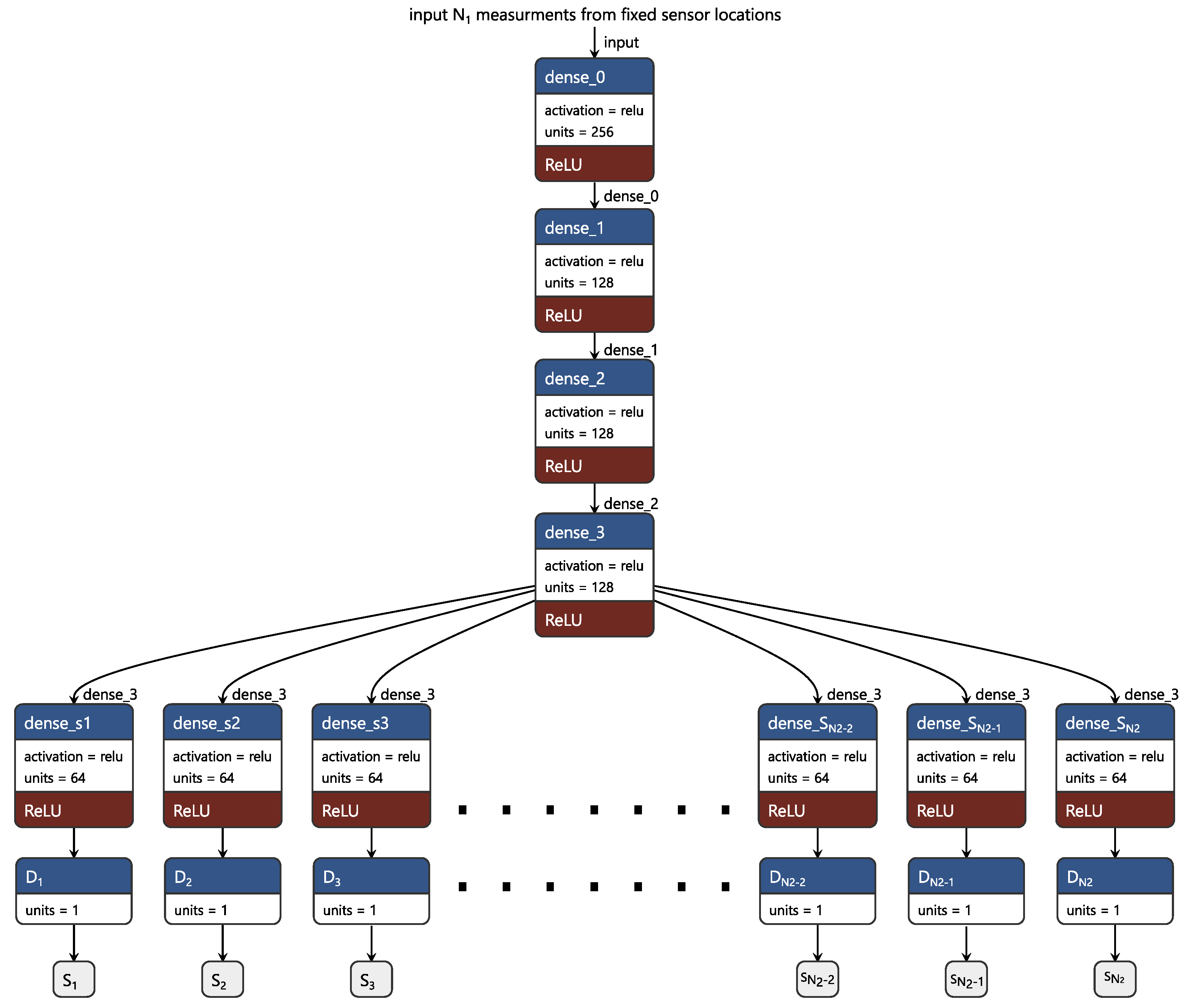Hence in this paper, based on the data collected from a greenhouse used to cultivate strawberries in [25], a framework based on the multi-channeled dense neural network (DNN) is proposed to be used to predict temperature and relative humidity values corresponding to the optimal sensor locations of each month without the need of moving the sensor from one location to another. Specifically, temperature and relative humidity values measured from the fixed locations (say the optimal locations of February) are used to predict the temperature and relative humidity values corresponding to the optimal locations of the other months referred to as target months (March, April, May, June, July, and October). The prediction of the temperature and relative humidity values corresponding to the optimal locations corresponding to the target month will help better estimate the micro-climates of the greenhouse. The effectiveness of the proposed model to predict temperature and relative humidity is demonstrated in terms of the resulting RMSE values. Furthermore, it is shown that the true and predicted sensor values are highly correlated based on Pearson’s correlation coefficient. Overall the results obtained show that the proposed framework is efficient and applicable in predicting micro-climates within protected cultivation systems and also comes with the advantage of cost reduction.In addition, as the prediction is performed for each month using the same fixed locations, the proposed framework alleviates the issue related to shifting of the sensors with the change in the external weather conditions. In other words, the novel framework proposed in this paper becomes an initiative basis in the research community for modeling dynamic optimal sensor placement in cultivation systems based on fixed sensors. Finally, it is important to note that the choice of the multi-channel DNN employed in this work is motivated by its simplicity in terms of implementation and deployment since it is well suited to several low-precision hardware for deep learning compared to other variants.

The rest of this paper is organized as follows: In Section 2, a review of related works is presented. Section 3 gives a brief description of the dataset and the associated pre-processing stages. In Section 4, the proposed framework and the associated model are presented. Section 5 presented the results and discussions, and finally, in Section 6 conclusions and future works are highlighted.

2. Review of Related Works

The prediction of micro-climates in protected cultivation systems under different setups has been studied in the literature [9,28,29,30]. The prediction models often employed range from very basic deterministic models [28] to more advanced learning networks such as ANN [9], multi-layer perceptron neural network (MLP-NN) [29], and extreme learning machine (ELM) [30]. Although these works propose the use of learning or deterministic models for micro-climate predictions, most of them applied these models to achieve different goals. For example, the deterministic model proposed in [28] was aimed at predicting crop temperature from measured air temperature, air density, and other related sensor-measured environmental conditions. The authors argued that rather than the air temperature, the crop temperature is responsible for crop growth and development. In [31], a dynamic model based on energy and mass transport processes, such as the mechanism of conduction, convection, radiation, etc., was employed to realize a prediction model capable of predicting the temperature of air in plant communities. Although the use of such models is very dependent on the structure of the greenhouse model, the authors claimed that the proposed model can be extended for a general greenhouse micro-climate prediction model. In terms of the use of learning networks, Liu et al. [30] proposed the use of ELM for predicting temperature and relative humidity from historical samples of indoor temperature and humidity. In order words, the learning model is aimed at predicting current micro-climates based on previously sampled or measured micro-climates. This is beneficial in situations where the cost of continually measuring micro-climates in terms of energy and communication protocols is high and needs to be minimized. In [9,29], where MLP-NN and ANN were employed, respectively, the aim of the models was to predict indoor or internal micro-climates based on measured external micro-climates such as temperature, relative humidity, wind speed, etc. Although the aforementioned works have considered the prediction of micro-climates in the greenhouse setting, the aims of their predictions are different from ours, where we predict the measurements of micro-climates at varying optimal sensor locations using input data from fixed-placed sensors.

Generally, it can be observed that most of the aforementioned models are relatively not computationally expensive. This is because the choice of model or learning networks for such applications is usually motivated by the nature of the underlying data (real-valued vectors) and the need for quick prediction or low inference time. In a similar fashion, we employ a simple multi-channel learning model that extracts global features from all the input data, which are consequently fed into the channels’ response for extracting local features corresponding to micro-climate measurements from different sensor locations.

3. Data Description and Pre-Processing

The dataset [25] employed in the current work contains sensor readings corresponding to internal temperature and relative humidity from 56 two-in-one sensors distributed within a greenhouse used to cultivate strawberries in Daegu, South Korea. The readings were collected for seven months (February, March, April, May, June, July and October). In [25], the same dataset was used to rank the sensor locations corresponding to each of the seven months. A more detailed description of the protected cultivation facility in terms of size and materials from which the data were collected, the type of sensors used, and how the 56 sensors were distributed within the greenhouse are provided in [25].

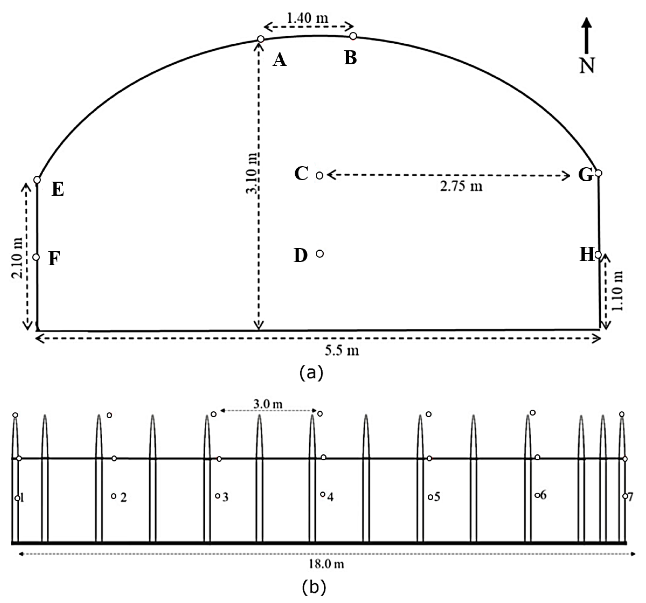
In Figure 1, the overall layout of the sensors in the considered greenhouse is provided. In addition, the sensor locations corresponding to temperature (T) and relative humidity (RH) corresponding to each month are ranked based on their ability to estimate the micro-climates of the greenhouse [25]. Due to space constraints, we only present the top 10 ranked sensor locations for each month in

Table 1. Locations of 10 top-ranked sensors corresponding to different months for temperature (T) and relative humidity (RH).

Rank	Optimal Locations
		February		March		April		May		June		July		October
	T	RH	T	RH	T	RH	T	RH	T	RH	T	RH	T	RH
1	E3	B4	G1	D6	A4	E4	D1	B2	E7	E2	B4	D3	A4	E4
2	F7	F5	C7	G6	E7	D2	B2	A3	C7	E6	D5	B6	E7	D2
3	D1	A1	B6	C4	F7	E3	F5	F6	F6	B2	G7	C3	F7	E3
4	D7	C1	A3	A2	A1	A2	C1	F7	D7	F7	G6	D6	A1	A2
5	E2	C5	D1	D3	E6	E6	D7	G6	G1	H3	E1	D7	E6	E6
6	C4	F2	E2	E6	D2	E5	A7	E3	E1	G6	E7	F5	D2	E5
7	H2	F3	D2	E1	F6	A4	C5	B4	G7	H1	D7	A3	F6	A4
8	E7	H5	B3	F4	G7	D3	F2	H1	B2	B1	G1	C2	G7	D3
9	G1	E2	C1	B4	G6	A5	F3	B1	A2	A6	F7	F4	G6	A5
10	E1	F1	E1	A5	D6	F2	A3	D7	E3	E4	A1	G3	D6	F2

. A detailed ranking of the 56 sensors for each month can be found in [25].

In the current work, we assume that $N_1$ sensors are fixed at $N_1$ top-ranked locations (referred to as optimal locations) corresponding to the month of February, as shown in Table 1. It should be noted that the optimal locations corresponding to temperature and relative humidity are different. Therefore, the fixed sensor locations for measuring temperature and relative humidity would be different. By observing the measurements obtained at these fixed locations, the goal is to develop a model that can predict the measurements corresponding to the $N_2$ optimal locations of the target month (say March). By doing so, the micro-climates of the greenhouse in the month of March, the target month, is accurately estimated without shifting the locations of the sensors. In other words, one prediction model is developed corresponding to each target month (March, April, May, June, July, and October). Therefore, the prediction accuracy of the models determines the precision of micro-climates estimation.

Since the model is expected to predict the values corresponding to the sensors at the $N_2$ optimal locations in the target months based on measurements from February, it is important to ensure consistency in comparison across the various months. Therefore, considering that the number of days in February is less, the length of the entire data samples is limited to those available in the month of February. Furthermore, the rows with missing sensor values were removed across all corresponding input and target months.

In terms of implementing the learning networks, the datasets were divided into training, validation, and test sets. The training and test set consists of 80 percent and 20 percent of the entire data, respectively, and 20 percent of the training data were used as the validation set. In order words, the dataset was divided, with 64%, 16%, and 20% of the entire dataset used for training, validation, and testing, respectively.

Table 2. Number of instances in train, validation, and test data.

Predicted Month	Temperature Data			Humidity Data
	Train	Test	Validate	Train	Test	Validate
March	16,711	5223	4178	16,252	5080	4064
April	16,283	5089	4071	16,516	5162	4130
May	16,639	5200	4160	16,343	5108	4086
June	15,264	4771	3816	15,270	4772	3818
July	14,954	4674	3739	15,160	4738	3791
October	15,549	4860	3888	16,031	5010	4008

provides a summary of the length of the training, test, and validation dataset. Furthermore, to ensure a faster convergence of the model, normalization of the input data based on the mean and standard deviation was performed. In the context of predicting sensor values, the input variable x is a $N_1$-dimensional vector comprising readings from $N_1$ temperature or relative humidity sensors for each case. The output y are $N_2$ real values corresponding to temperature or relative humidity values for the target months.

4. Methodology

4.1. Dense Neural Network (DNN)-Based Regression Model

Considering that the output is an $N_2$-dimensional vector where each element represents the sensor values corresponding to each of the $N_2$ optimal locations for the target month, a multi-channel DNN regression model is employed. In [32], a generalized approach to formalize any NN-based model can be found. In Figure 2, a generalized overview of the DNN architecture, where $N_1$ and $N_2$ are corresponding to the number of sensor locations considered at the input and output, respectively, is presented. Based on the target month, say March, the input to the networks is the temperature or relative humidity measurements taken at the $N_1$ optimal locations of February, which are considered as the fixed locations throughout the whole study. The input is passed through a series of 4 dense layers, namely, dense_0, dense_1 dense_2, and dense_3, as shown in Figure 2, which extract global features from all the $N_1$ input sensor values. These global features are then fed into $N_2$ different dense channels, the output of which represents the predicted sensor values corresponding to the $N_2$ optimal locations of the target month, March. Each of these $N_2$ dense channels helps extract the local features corresponding to each of the sensor locations. These dense channels consist of a single dense layer of 64 units with Relu activation functions and, consequently, a single-unit, dense layer as the output layer. Using the $N_1$ fixed locations, the learning model corresponding to each target month is trained for 200 epochs with a batch size of 64. The predicted values based on the proposed model are favorably compared with the real values corresponding to the target month in terms of the root mean square error (RMSE) and correlation coefficients.

4.2. Evaluation Metrics

To evaluate the proposed framework, we used two metrics, namely, root mean -squared error (RMSE) and Pearson’s correlation coefficient (R), as expressed in Equations (1) and (2), respectively.

$$RMSE=\sqrt{\frac{1}{N}\sum _{j=1}^N(e_t}{)}^2$$

(1)

where N is the number of test samples and $e_t$ is the error between the true and predicted sensor values.

$$R=\frac{\sum (x_i-\overline{x})(y_i-\overline{y})}{\sqrt{{\sum (x_i-\overline{x})}^2{(y_i-{\overline{y}}^{})}^2}}$$

(2)

where $x_i$ is the ith true sensor value, $\overline{x}$ is the mean of the true sensor values, $y_i$ is the ith predicted sensor value, and $\overline{y}$ is the mean of the predicted sensor values.

In addition, to evaluate the efficiency of the proposed framework, we provide RMSE values between the measured values (temperature and relative humidity) from the fixed sensor locations and the true measurements corresponding to the $N_2$ optimal sensors of the target month. In other words, we present the RMSE values, assuming that there exists no prediction model, as the one proposed in the current work. In addition, we present the percentage reduction in the RMSE values by comparing the RMSE values with and without the proposed DNN model.

5. Results and Discussion

The proposed model in this work was implemented and evaluated using Python and Keras installed on a computer with an Intel(R) Core(TM) i7, 2.60 GHz, 16 GB RAM, running Windows 10, 64-bit. The results from the experiments are presented in this section accordingly.

5.1. Temperature and Humidity Prediction RMSE

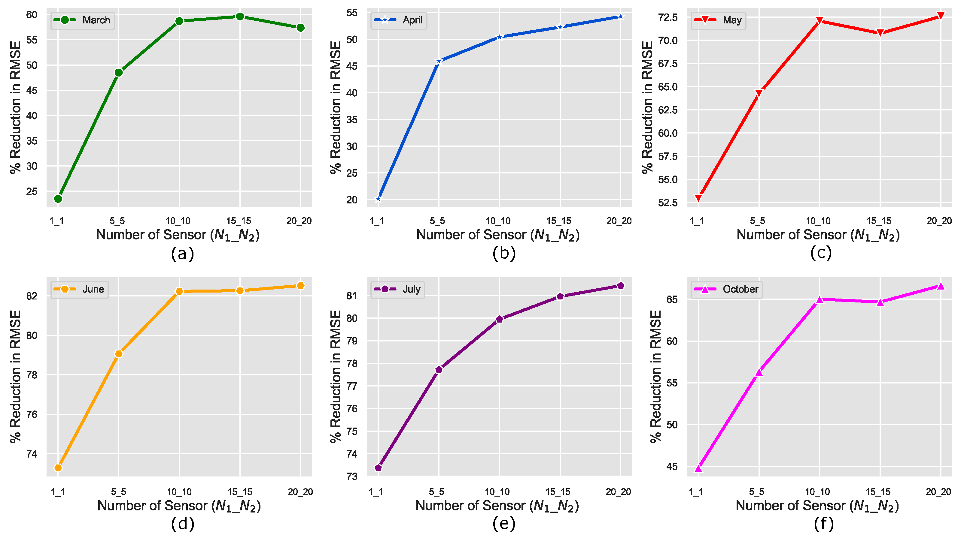
Based on different values of $N_1$ and $N_2$, the results of temperature prediction for all the six months are presented in

Table 3. Comparison of temperature prediction with and without DNN model in terms of RMSE for different values of $N_1$ and $N_2$.

Predicted Month	RMSE
	${\mathit{N}}_{\mathbf{1}}=\mathbf{1},{\mathit{N}}_{\mathbf{2}}=\mathbf{1}$			${\mathit{N}}_{\mathbf{1}}=\mathbf{5},{\mathit{N}}_{\mathbf{2}}=\mathbf{5}$			${\mathit{N}}_{\mathbf{1}}=\mathbf{10},{\mathit{N}}_{\mathbf{2}}=\mathbf{10}$			${\mathit{N}}_{\mathbf{1}}=\mathbf{15},{\mathit{N}}_{\mathbf{2}}=\mathbf{15}$			${\mathit{N}}_{\mathbf{1}}=\mathbf{20},{\mathit{N}}_{\mathbf{2}}=\mathbf{20}$
	DNN Model	W/O DNN Model	RMSE Reduction (%)	DNN Model	W/O DNN Model	RMSE Reduction (%)	DNN Model	W/O DNN Model	RMSE Reduction (%)	DNN Model	W/O DNN Model	RMSE Reduction (%)	DNN Model	W/O DNN Model	RMSE Reduction (%)
March	3.4313	4.486	23.5	2.2177	4.3059	48.49	1.7744	4.295	58.69	1.7274	4.27676	59.61	1.813	4.253	57.37
April	3.769	4.7207	20.16	2.8217	5.2158	45.9	2.4798	5.0001	50.41	2.3984	5.0265	52.28	2.2835	4.9931	54.27
May	4.879	10.3591	52.9	3.6129	10.0993	64.22	2.8061	10.051	72.08	2.9978	10.2512	70.76	2.8256	10.3058	72.58
June	4.5209	16.91844	73.28	3.4017	16.2493	79.06	2.9317	16.4949	82.23	2.8681	16.1764	82.26	2.8209	16.1334	82.52
July	3.555	13.3485	73.37	3.0707	13.7859	77.72	2.7632	13.7796	79.95	2.5978	13.6444	80.96	2.528	13.6213	81.44
October	3.9781	7.2066	44.8	3.2783	7.5076	56.33	2.6372	7.5388	65.01	2.6396	7.4724	64.68	2.4957	7.4801	66.64

in terms of RMSE. Furthermore, the table includes the resulting RMSE of the sensor readings without the DNN model as well as the percentage error margin incurred with the DNN model compared with those without the DNN model. The resulting RMSE values, as presented in Table 3, is indicative that the error associated with the proposed DNN-based prediction of the temperature values from the optimal sensor locations in each month is significantly lower than those measured without the DNN model. Specifically, the proposed framework, which is based on the DNN model results in a 68.67% reduction in the average RMSE over all the five months compared to those obtained without the DNN model.

In [25], the optimal sensor locations were identified based on the ranking of all the 56 sensors distributed within the greenhouse. Consequently, $N_2=10$ sensors were selected. However, there was no clear analysis to justify why only $N_2=10$ sensors were selected as the optimal number of sensors. Since the DDN-based prediction of the greenhouse micro-climates is superior to those without the DNN model, we provide further analysis based on the DNN model. Specifically, to show the effect of using different numbers of input ($N_1$) and output ($N_2$) sensors, we present a graphical illustration of the percentage reduction in error incurred with the DNN model for $N_1$ = $N_2$ = 1, 5, 10, 15, and 20 for each month, respectively, in Figure 3. From the figure, it is clear from the error curves that the knee or saturation point is the $N_1$ = $N_2$ = 10 for all the months. This is because a drastic increase in error reduction is observed from $N_1$ = $N_2$ = 1 to $N_1$ = $N_2$ = 10. However, as the values of $N_1$ = $N_2$> 10, the percentage improvement saturates. This might be because of the fact that adding more sensors may not provide any extra information that can help better estimate the micro-climates of the greenhouse. This validates the selection of 10 highly ranked sensors as optimal in [25].

In

Table 4. Comparison of relative humidity prediction with and without DNN model in terms of RMSE for different values of $N_1$ and $N_2$.

Predicted Month	RMSE
	${\mathit{N}}_{\mathbf{1}}=\mathbf{1},{\mathit{N}}_{\mathbf{2}}=\mathbf{1}$			${\mathit{N}}_{\mathbf{1}}=\mathbf{5},{\mathit{N}}_{\mathbf{2}}=\mathbf{5}$			${\mathit{N}}_{\mathbf{1}}=\mathbf{10},{\mathit{N}}_{\mathbf{2}}=\mathbf{10}$			${\mathit{N}}_{\mathbf{1}}=\mathbf{15},{\mathit{N}}_{\mathbf{2}}=\mathbf{15}$			${\mathit{N}}_{\mathbf{1}}=\mathbf{20},{\mathit{N}}_{\mathbf{2}}=\mathbf{20}$
	DNN Model	W/O DNN Model	RMSE Reduction (%)	DNN Model	W/O DNN Model	RMSE Reduction (%)	DNN Model	W/O DNN Model	RMSE Reduction (%)	DNN Model	W/O DNN Model	RMSE Reduction (%)	DNN Model	W/O DNN Model	RMSE Reduction (%)
March	14.2951	16.6314	14.05	12.0131	16.1924	25.81	10.5982	16.1097	34.21	10.7687	16.13353	33.25	10.4168	16.0724	35.19
April	14.1778	22.7773	37.75	12.7681	22.8833	44.2	13.0693	22.18422	41.09	10.5447	21.63	51.25	10.8462	21.8471	50.35
May	17.6504	26.2172	32.68	17.0076	26.8919	36.76	15.3399	26.9629	43.11	14.4252	26.359	45.27	13.81256	26.35056	47.82
June	15.5105	32.1841	51.81	14.0204	32.4554	56.8	13.6979	32.4173	57.75	13.28	32.1747	58.73	13.4313	32.08896	58.14
July	11.7474	24.05563	51.17	11.77418	24.092	51.13	10.9207	24.2066	54.89	10.4535	23.9932	56.43	10.61337	23.9488	55.68
October	14.1119	23.4509	39.82	13.0888	23.126	43.4	12.363	23.1641	46.63	12.677	23.6228	46.34	12.6537	23.714	46.64

, the results of humidity prediction for all the associated months are presented in terms of RMSE. The table further includes the resulting RMSE of the sensor readings obtained without the DNN model. In terms of the RMSE, the results show that there is a 46.21% overall reduction in error of the predicted humidity values based on the DNN-based framework compared to those obtained without the DNN model. In addition, the percentage improvement in the measurement error of relative humidity follows a similar pattern to the temperature, as shown in Figure 3.

5.2. Correlation Coefficients

Correlation results based on Pearson’s correlation coefficients between the real sensor value readings and predicted sensor value readings are shown in

Table 5. Performance comparison of proposed DNN framework for different $N_1$ and $N_2$ in terms of Pearson correlation coefficient.

Predicted Month	Correlation Coefficients
	${\mathit{N}}_{\mathbf{1}}=\mathbf{1},{\mathit{N}}_{\mathbf{2}}=\mathbf{1}$		${\mathit{N}}_{\mathbf{1}}=\mathbf{5},{\mathit{N}}_{\mathbf{2}}=\mathbf{5}$		${\mathit{N}}_{\mathbf{1}}=\mathbf{10},{\mathit{N}}_{\mathbf{2}}=\mathbf{10}$		${\mathit{N}}_{\mathbf{1}}=\mathbf{15},{\mathit{N}}_{\mathbf{2}}=\mathbf{15}$		${\mathit{N}}_{\mathbf{1}}=\mathbf{20},{\mathit{N}}_{\mathbf{2}}=\mathbf{20}$
	Temperature	Humidity	Temperature	Humidity	Temperature	Humidity	Temperature	Humidity	Temperature	Humidity
March	0.87	0.85	0.93	0.93	0.96	0.94	0.96	0.94	0.95	0.95
April	0.82	0.89	0.92	0.91	0.95	0.93	0.95	0.95	0.95	0.94
May	0.69	0.76	0.82	0.78	0.89	0.82	0.89	0.84	0.9	0.86
June	0.79	0.76	0.87	0.80	0.92	0.81	0.92	0.82	0.91	0.82
July	0.56	0.66	0.78	0.72	0.82	0.75	0.85	0.79	0.84	0.78
October	0.73	0.8	0.85	0.83	0.911	0.84	0.92	0.84	0.92	0.84

. From the table, it can be observed that the predicted sensor values are highly correlated with the true sensor values by an average correlation value of 0.91 and 0.85 for temperature and humidity, respectively. These average correlation values are comparable with those from the literature, where the correlation coefficients generally range between 0.977 to 0.980 and 0.825 to 0.967 for temperature and relative humidity, respectively [9,33].

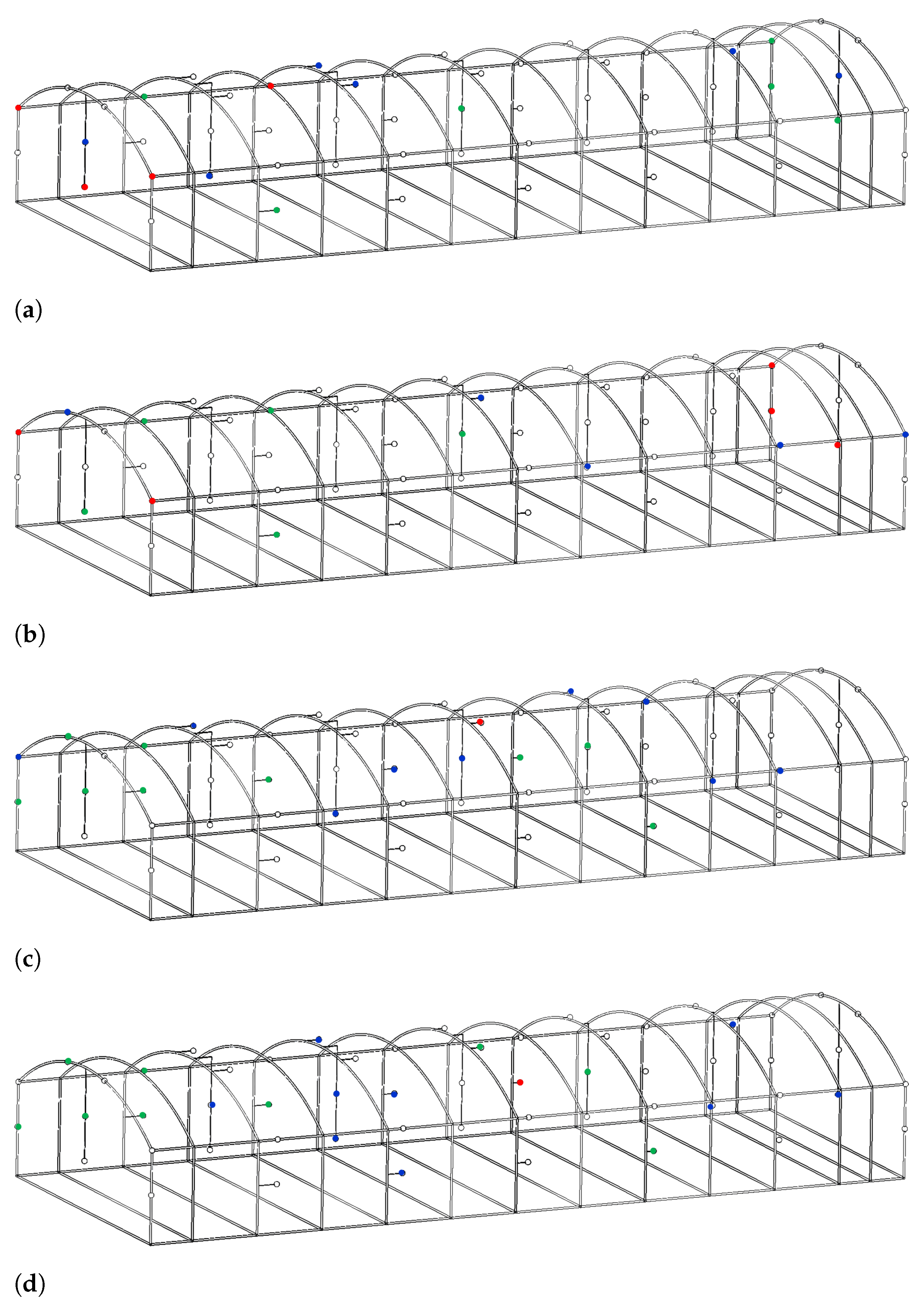
Furthermore, both temperature and humidity show a similar correlation trend, where the highest values of 0.95 and 0.94 are obtained in the month of March, while the lowest values of 0.82 and 0.75 are obtained in the month of July, respectively. This can be attributed to how the optimal sensor locations of March and July are distributed relative to the fixed sensor locations. In Figure 4, the fixed sensor locations (green) and optimal sensor locations of target months (March and July) are highlighted (glue) for both temperature and humidity to show the effect of the respective locations in the overall percentage of error reduction. In addition, the optimal locations of the target month (March and July) that overlap with some of the fixed locations are depicted in red.

As depicted in Figure 4a,b, the target months of March and July have four and five overlapping temperature sensor locations with respect to the fixed locations, respectively. Furthermore, as shown in the figure, the sensor locations of March compared to the fixed locations are closer, and for each of the fixed locations, there are also representative locations in March in the same region. However, in July, the sensor locations are much farther from those of the fixed locations when compared with those in March. Therefore, the proximity of the optimal sensor locations of the target month March with respect to the fixed locations resulted in a higher correlation compared to that of July.

Similarly, in terms of humidity, although both March and July have only one overlapping sensor location with fixed locations, as shown in Figure 4c,d, it is clear that the high correlation in March can be associated with the observation that the sensors are well distributed in regions close to the fixed locations. On the other hand, the sensor locations of July are simply packed in regions where none of the fixed sensors are located.

5.3. Effect of Number of Fixed Sensor Locations on the Prediction Accuracy of DNN Model

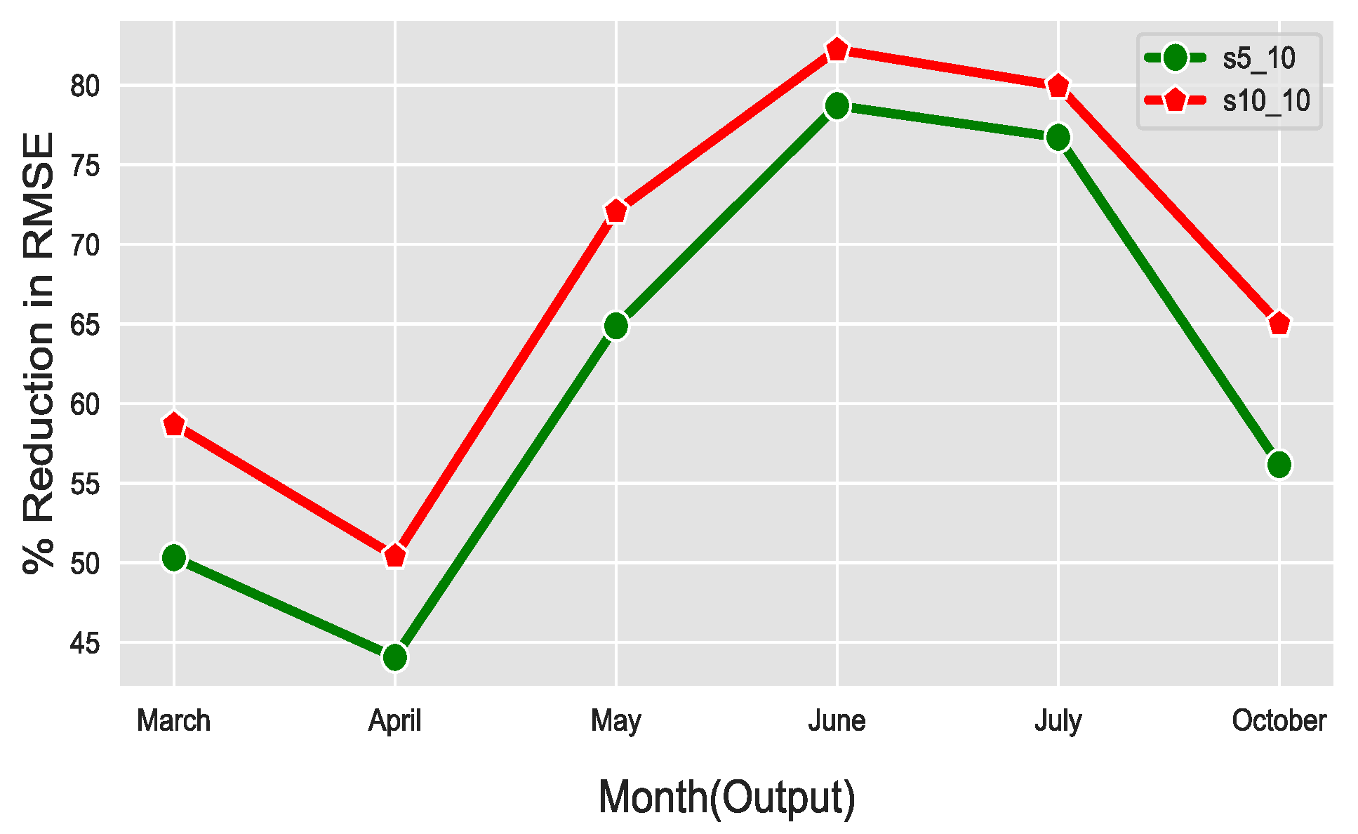
In the previous section, the analysis was conducted considering that the input and output dimensions, $N_1$ and $N_2$, respectively, are equal ($N_1$ = $N_2$). However, it would be interesting to investigate instances where $N_1<N_2$ as this would help to facilitate decisions related to the trade-off between cost and accuracy of estimation. Specifically, the input dimension $N_1$ is directly related to cost, while the output dimension N is directly proportional to the accuracy of prediction, thus providing a better estimation of micro-climates. In other words, since $N_1$ is the number of sensors that would be installed, as the number of $N_1$ sensors increases, the cost also increases. On the other hand, as the number of $N_1$ increases, the accuracy of prediction tends to increase until saturation is reached.

Table 6. Effect of number of sensors ($N_1$) on the temperature prediction accuracy of DNN model in terms of RMSE.

Predicted Month	RMSE
	${\mathit{N}}_{\mathbf{1}}=\mathbf{5},{\mathit{N}}_{\mathbf{2}}=\mathbf{10}$	${\mathit{N}}_{\mathbf{1}}=\mathbf{10},{\mathit{N}}_{\mathbf{2}}=\mathbf{10}$
	DNN Model	DNN Model	W/O DNN Model
March	2.1337	1.7744	4.295
April	2.811	2.4798	5.0001
May	3.5302	2.8061	10.051
June	3.5121	2.9317	16.4949
July	3.2077	2.7632	13.7796
October	3.305	2.6372	7.5388

summarizes the RMSE values for different combinations of the input and output number of sensors. From Table 6, we can observe that the prediction accuracy of the DNN model, where the input of 10 sensors is provided is better compared to the prediction of the DNN model with only 5 input measurements. However, the prediction accuracy of the DNN model that employs five input measurements is better than the measurements taken from fixed sensors (or without the DNN model). In other words, it is intuitive that installing more sensors can help estimate the environment better, as clearly depicted in Figure 5, but it is expensive. Therefore, the best way is to use fewer sensors and use the model proposed so that the environment can be better estimated by predicting the values of the sensors at top preferred locations.

The above analysis was conducted with respect to the temperature measurement in the greenhouse. However, a similar observation was made with respect to the measurement of relative humidity in the greenhouse.

6. Conclusions

In order to alleviate the need to move sensors from one dynamic optimal sensor location to another due to changes in the external weather condition, this study proposes a framework based on multi-channel dense neural network regression model for predicting micro-climates corresponding to changing sensor locations using measurements from fixed sensors. Results of micro-climate predictions obtained based on the proposed framework were comparable with the true sensor measurements corresponding to the dynamic sensor locations. Specifically, the proposed framework in terms of RMSE achieved a 68.67% reduction in error for temperature and 46.21% overall reduction in error for relative humidity compared with a setup without the proposed models. In terms of the Pearson correlation coefficient, the result showed a high correlation, with an average of 0.91 and 0.85 for temperature and relative humidity, respectively. The highest correlation values of 0.95 and 0.94 for temperature and relative humidity, respectively, obtained in the month of March and lowest values of 0.82 and 0.75 for temperature and relative humidity obtained in the month of July, can be explained as a result of the distance between the test month’s (February) data and the respective predicted months. The deployment of the proposed framework would generally facilitate accurate monitoring and control of micro-climates in protected cultivation systems. Although the current work is limited to monthly variations of optimal sensor locations, investigating the proposed framework for intraday variations would be of interest in the future.