
Global Dynamics of Viral Infection with Two Distinct Populations of Antibodies

1
Department of Mathematics, Faculty of Science, King Abdulaziz University, P.O. Box 80203, Jeddah 21589, Saudi Arabia
2
Department of Mathematics, Faculty of Science, King Khalid University, Abha 62529, Saudi Arabia
3
Department of Mathematics, College of Science, Taif University, P.O. Box 11099, Taif 21944, Saudi Arabia
*
Author to whom correspondence should be addressed.
Mathematics 2023, 11(14), 3138; https://0-doi-org.brum.beds.ac.uk/10.3390/math11143138
Submission received: 4 June 2023
/
Revised: 10 July 2023
/
Accepted: 13 July 2023
/
Published: 16 July 2023
(This article belongs to the Special Issue Mathematical Advances in Studying Rare and Novel Diseases)
Abstract
:This paper presents two viral infection models that describe dynamics of the virus under the effect of two distinct types of antibodies. The first model considers the population of five compartments, target cells, infected cells, free virus particles, antibodies type-1 and antibodies type-2. The presence of two types of antibodies can be a result of secondary viral infection. In the second model, we incorporate the latently infected cells. We assume that the antibody responsiveness is given by a combination of the self-regulating antibody response and the predator–prey-like antibody response. For both models, we verify the nonnegativity and boundedness of their solutions, then we outline all possible equilibria and prove the global stability by constructing proper Lyapunov functions. The stability of the uninfected equilibrium and infected equilibrium is determined by the basic reproduction number . The theoretical findings are verified through numerical simulations. According to the outcomes, the trajectories of the solutions approach and when and , respectively. We study the sensitivity analysis to show how the values of all the parameters of the suggested model affect under the given data. The impact of including the self-regulating antibody response and latently infected cells in the viral infection model is discussed. We showed that the presence of the self-regulating antibody response reduces and makes the system more stabilizable around . Moreover, we established that neglecting the latently infected cells in the viral infection modeling leads to the design of an overflow of antiviral drug therapy.
MSC:
34D20; 34D23; 37N25; 92B051. Introduction
Recently, the world witnessed the spread of many infectious viruses, which caused many deaths, and which negatively affected public health and the global economy. Scientists and researchers in various fields have made great efforts to study how to confront these viruses and eliminate the diseases resulting from them. Mathematical modeling is considered an effective and powerful method for understanding the within-host (or between-host) dynamics of several human viruses. Mathematical models have been used to provide useful insights for the development of new antiviral drug treatments. Examples of these viruses are as follows:
The basic model of viral infection was introduced by Nowak and Bangham [8] by considering the interaction of three compartments, target cells (x), infected cells (y) and free viruses (v). When foreign bodies enter the human body, the immune system becomes active against these bodies. Antibodies and cytotoxic T lymphocytes (CTLs) play major roles in fighting viruses. Antibodies are produced from the B cells and neutralize viruses. CTLs are responsible for killing the infected cells. Wodarz et al. [25] incorporated the influence of antibodies into the viral infection model as in the following:
where is the concentration of antibodies. Parameters , , , , , , , and are positive. The model was extended by including, (i) time delay [26,27,28,29], (ii) cell-to-cell transmission [30], (iii) latently infected cells [31] and (iv) age structure [32,33,34].
Equation (4) can be generalized as:
where is a general function that represents the antibody responsiveness. Several forms of have been presented in the literature such as:
All the mathematical models given above are formulated for primary viral infection. In this case, it is assumed that the virus is attacked by one type of antibody. It may happen that there are two distinct populations of antibodies against a viral infection. For example, in the case of DENV infection, there are four DENV serotypes that can infect the human [39]. When a person is infected for the second time with another type of DENV serotype, there are two types of antibodies, a heterologous (nonspecific) antibody previously formed on the primary infection and a homologous (strain-specific) antibody against the new DENV serotype of the secondary infection. Gujarati and Ambika [40] formulated a secondary DENV infection model with two types of antibodies. Elaiw and Alofi [37] and Raezah [38] extended the model presented [40] by considering the spatial dependence. In [37,38], the antibody responsiveness is given by , where the antibodies are available just when the infection occurs. On the other hand, it was assumed in [10,15,41] that the antibodies are available even if there is no infection.
The aim of this paper is to develop two virus dynamics models with two types of antibodies, and . In the case of secondary viral infection, and can be the populations of nonspecific and strain-specific antibodies, respectively. We assume that both types of antibodies, and , are at levels and , respectively, in the absence of infection, with and being the sources [10,15,42]. We model this by assuming the expansion of the populations and at rates and , respectively. In this case, the antibody responsiveness function is given by the self-regulating antibody response and the predator–prey-like antibody response i.e., , . The second model is an extension of the first one by considering two classes of viral-infected cells, latently infected cells (which contain the viruses but are not producing them) and actively infected cells (which produce the viruses). For the proposed models, basic properties are established such as the solutions’ nonnegativity and boundedness. We derive the basic reproduction number (or and the prospective equilibrium points with the conditions of their existence. We examine the global stability of the equilibria by using appropriate Lyapunov functions and applying the Lyapunov–LaSalle asymptotic stability (L-LAS) theorem. Finally, some numerical simulations are carried out to test the key parameters’ impact on the models’ dynamics and to ensure the theoretical results. We also study the sensitivity analysis to show how the values of all the parameters of the suggested model affect (or under the given data.
2. Model with Two Antibodies
We formulate a virus dynamics model with two types of antibodies and :
where is the concentration of antibodies type-i, . In the following, we study the basic and global properties of the model.
2.1. Preliminary Results
First, we determine a bounded region for the model’s solutions to illustrate the biological acceptability of the proposed model. In particular, the concentrations of cells and viruses should not become negative or unbounded. Let , be defined as:
where . We define a region as:
and be the interior of .
Lemma 1.
Solutions of system (5)–(9) are positively invariant and bounded in Ξ.
Proof.
We have
Thus, all solutions of system (5)–(9) with initial satisfy (see Proposition B.7 of [43]). Define a function as:
then
Hence, , if . This implies that , , and if . □
Lemma 2.
There exists a threshold parameter such that (i) if then there exists a unique uninfected equilibrium , (ii) if then there exists an infected equilibrium besides .
Proof.
Let the R.H.S. of Equations (5)–(9) be zero
From Equations (10), (11), (13) and (14), we have
Substituting in Equation (12), we obtain
Equation (16) has two possibilities, the first is which gives the infection-free equilibrium , where , and . The other possibility of Equation (16) is and
which gives
where
We define a function , then we obtain
We have if the following condition is satisfied
Observe that
Hence,
We note from Equation (15) that the solution gives or ; moreover, yields and . Therefore, the only acceptable solution is , which gives
We define the basic reproduction number as:
Then, the infected equilibrium exists when . Here, represents the total number of those newly infected that arise from any one infected cell at the beginning of infection [10]. □
2.2. Global Stability
In this section, we prove the global stability of the two equilibria of system (5)–(9). The global stability of these models is established using a Lyapunov approach, which is closely related to the one given by Korobeinikov [44], Korobeinikov and Wake [45] and Elaiw [46] by constructing explicit Lyapunov functions, which are extensions and modified forms of the Lyapunov functions given in [44,45,46].
Define a function and let be the largest invariant subset of , . We use the arithmetic mean–geometric mean inequality [47]:
Theorem 1.
- (i)
- The uninfected equilibrium is globally asymptotically stable (G.A.S) in Ξ if ,
- (ii)
- is unstable if .
Proof.
- (i)
- DefineWe observe that for all and . Calculating along the solutions of (5)–(9) as:Using , and , we obtainIf , then , for all . Moreover, when , , and for all t. The solutions of system (5)–(9) converge to [48]. The set has elements satisfying , , and . We find from Equation (7) that
- (ii)
- The Jacobian matrix of system (5)–(9) is calculated as:Then, the characteristic equation at the equilibrium is given bywhere is the eigenvalue andClearly if , then and Equation (20) has a positive root, and hence, is unstable.
□
The result of Theorem 1 established that, if there are some control strategies (such as using some types of antiviral drug therapies) which make , then the viruses will be cleared from the body regardless of the initial states.
Theorem 2.
The infected equilibrium is G.A.S in if .
Proof.
Define
Calculating along the trajectories of (5)–(9):
Applying the equilibrium conditions
we obtain
and
From the equilibrium conditions, we have and . It follows that
Applying inequality (19) we obtain
Consequently, for all . Moreover, when and thus . L-LAS theorem implies that is G.A.S in . □
Theorem 2 suggests that, if , then a chronic viral infection will be established regardless of the initial states.
Remark 1.
In some cases, one can consider a more complex within-host virus dynamics model with n-compartments (Target cells, infected cells, free viruses, immune cells, etc.), . However, it seems that the following Lyapunov function can be successfully applied to establish the global stability of an equilibrium :
where are positive constants and
3. Model with Latency
In this section, we consider two populations of viral-infected cells, latently infected cells and actively infected cells. We assume that a fraction of infected cells become active and the remaining () become latent. Let be the concentration of latently virus-infected cells at time t. The model with latency can be formulated as:
The latently infected cells are activated at rate and die at rate .
3.1. Preliminary Results
Let , be defined as:
where . Define a domain as:
Lemma 3.
Solutions of system (21)–(26) are positively invariant and bounded in .
Proof.
We have
Hence, all solutions of system (21)–(26) with initial satisfy . Let
then
Hence, if . This implies that , , and if . □
Lemma 4.
There exists a threshold parameter such that (i) if then there exists a unique uninfected equilibrium , (ii) if then there exists an infected equilibrium as well as .
Proof.
The equilibrium points of system (21)–(26) are calculated by solving the following equations:
From Equations (27)–(29), (31) and (32), we have
Substituting in Equation (30) we obtain
Equation (34) has two possibilities, the first is , which gives the infection-free equilibrium , where , and . The other possibility of Equation (34) is and
where
Let , then we obtain
We have when
We note that
From Equation (33), the solution yields or ; moreover, gives and . Therefore, the only acceptable solution is , which provides
The basic reproduction number of model (21)–(26) can be defined as:
Then the infected equilibrium with immunity exists when □
3.2. Global Stability
Define a function and let be the largest invariant subset of , .
Theorem 3.
- (i)
- If then the uninfected equilibrium of system (21)–(26) is G.A.S in ,
- (ii)
- if , then is unstable.
Proof.
- (i)
- DefineObserve that for all and Calculating along the solutions of (21)–(26) as:Using , and we obtainTherefore, if , then for all . Moreover, when , , and for all t. The solutions of system (21)–(26) converge to , which contains elements that satisfy , , and . It follows from Equation (24) thatFurthermore, from Equation (23) we haveHence, and L-LAS theorem provides that is G.A.S in .
- (ii)
- The Jacobian matrix of system (21)–(26) is calculated as:Then, the characteristic equation at the equilibrium is given bywhere is the eigenvalue andClearly, if , then and Equation (37) has a positive root, and hence, is unstable.
□
Theorem 4.
The infected equilibrium of system (21)–(26) is G.A.S in if .
Proof.
Define
Calculating along the trajectories of (21)–(26):
The equilibrium conditions of imply
Then, we obtain
and
With more simplifications we obtain
The equilibrium conditions give and . Hence
From inequality (19) we obtain for all . Furthermore, when . This gives , and according to L-LAS theorem, is G.A.S in . □
4. Numerical Simulations
4.1. Numerical Simulations for Model (5)–(9)
In this subsection, we present numerical simulation to confirm the global stability of equilibria for system (5)–(9) using the values given in Table 1.
Stability of Equilibria
We simulate system (5)–(9) using the following initials:
IS-1:,
IS-2:
IS-3:.
We note that, due to the difficulty of obtaining real data from viral-infected patients with two types of active antibodies, we therefore take arbitrary initial conditions in solving the system numerically. The global stability results given in Theorems 1 and 2 ensure that the solutions of system (5)–(9) converge to either uninfected equilibrium (when ) or infected equilibrium (when ) regardless of the chosen initial values.
Selecting different values of under the above initial conditions leads to the following cases:
Case 1 (Stability of ): We take . For this case, we have Figure 1 shows that the solutions with initials IS-1, IS-2 and IS-3 reach the uninfected equilibrium . According to the Theorem 1, is G.A.S. In this case, the virus will die out and the number of target cells will return to its normal level.
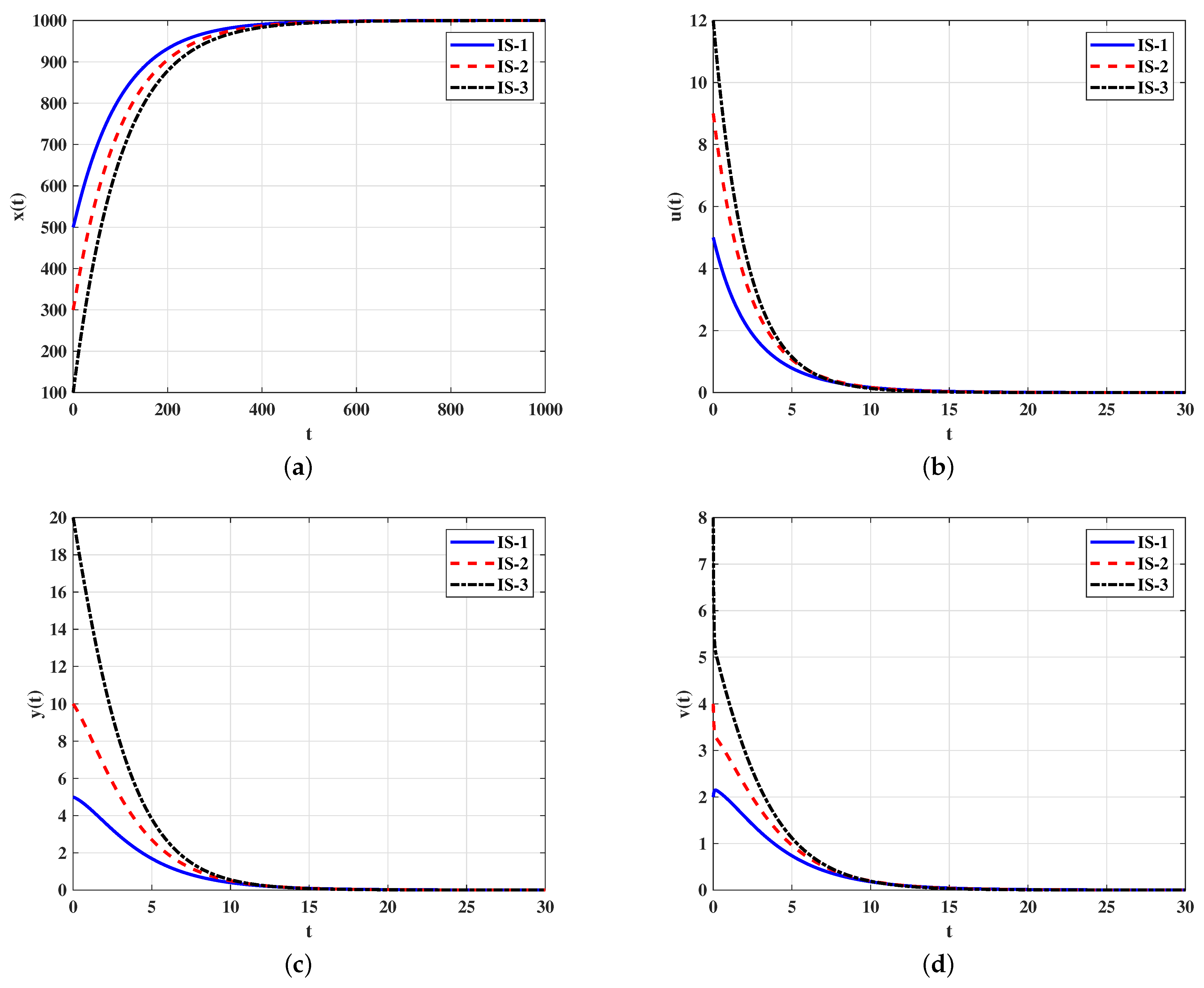
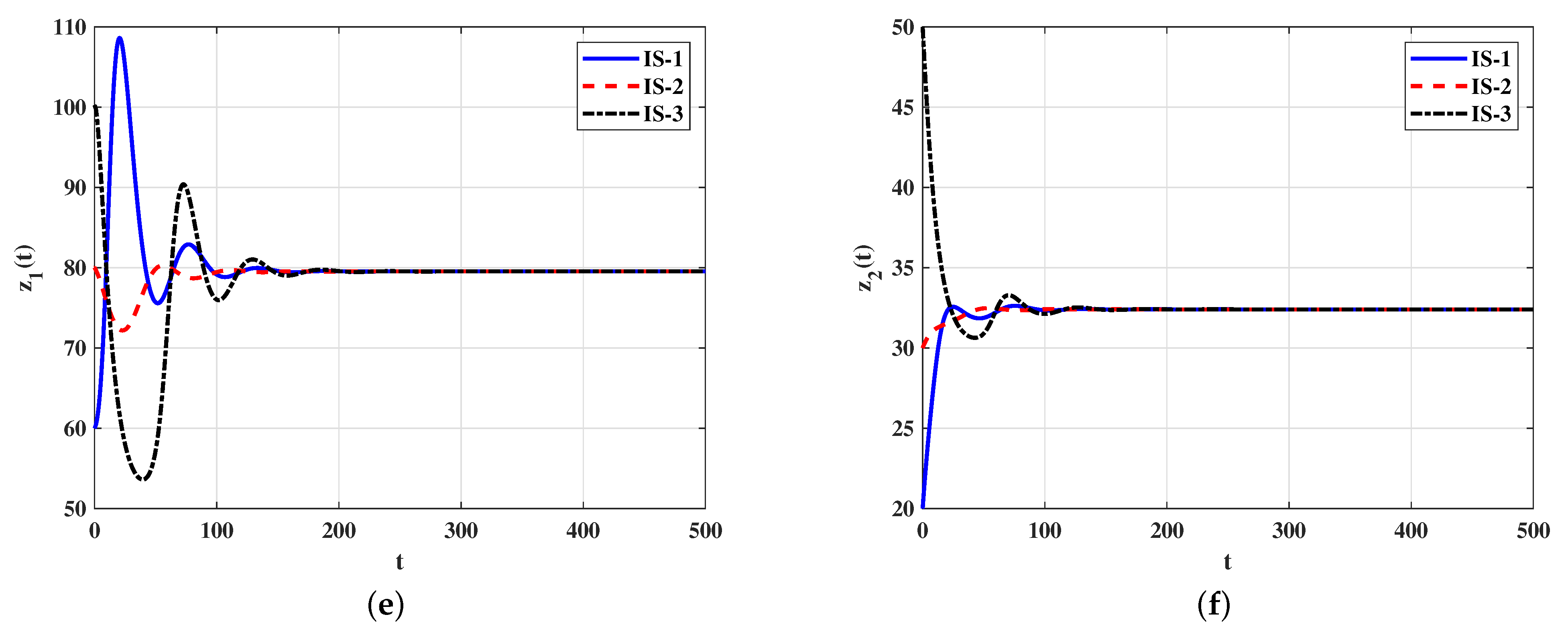
Case 2 (Stability of ): By choosing , we obtain . Figure 2 displays that the solutions starting with initials IS-1, IS-2 and IS-3 tend to the infected equilibrium . Lemma 2 and Theorem 2 state that exists and it is G.A.S. This strategy will lead to chronic viral infection.
4.2. Numerical Simulations for Model (21)–(26)
We present a numerical simulation for system (21)–(26). We consider the values of the parameters given in Table 1 and the following parameters: and .
4.2.1. Sensitivity Analysis
When modeling complicated interactions, sensitivity analysis is particularly important in pathology and epidemiology [52]. Our ability to control the spread of disease or crime can be determined by analyzing sensitivities. It is possible to calculate sensitivity indexes in three ways: directly through direct differentiation, using a Latin hypercube sampling method or by linearizing the model and solving the resulting equations [52,53].
The indices can be expressed analytically in this study using direct differentiation. By using partial derivatives, you can calculate the sensitivity index when variables vary based on parameters. In terms of the parameter, the normalized forward sensitivity index of is expressed as follows:
where is a given parameter. The sensitivity indices for each parameter included in are calculated using Equation (39). For instance, the sensitivity index of the parameter value with respect to is computed as:
Table 2 and Figure 3 display the value of the sensitivity index of based on the parameter values in Table 1. Clearly, , , , , , and have positive indices. In terms of sensitivity, , and are the most important parameters and is the least important. In this case, there is a positive relationship between the endemicity of the disease and the increase in the values of these parameters , , , , , and , while keeping other parameters constant. The remaining indices are negative, i.e., the value of decreases as the values of , , , , , , and increase. The parameters of antibody responsiveness, and , do not affect .
4.2.2. Stability of Equilibria
We choose three different initial states as follows:
IS-1:,
IS-2:
IS-3:.
Selecting different values of under the above initial states leads to the following cases:
Case 1 (Stability of ): We consider . For this case, we obtain Figure 4 illustrates that the solutions with initials IS-1, IS-2 and IS-3 reach the equilibrium This shows that is G.A.S according to Theorem 7. In this situation, the infected cells and virus particles will die out.
Case 2 (Stability of ): We select This gives . In Figure 5, we show that the solutions starting with initials IS-1, IS-2 and IS-3 tend to and then it is G.A.S which agrees with Theorem 8.
5. Discussions
In this section, we discuss the effect of including the self-regulating antibody response and latently infected cells on the virus dynamics. To address the influence of including the self-regulating antibody response in the viral infection model. We compare the basic reproduction number of system (1)–(4) where the self-regulating antibody response is not included and that of system (5)–(9). The basic reproduction number of model (1)–(4) can be calculated as:
Clearly,
Therefore, the presence of the self-regulating antibody response reduces the basic reproduction number and then makes the system more stabilizable around the uninfected equilibrium .
To discuss the impact of incorporating the latently infected cells in the model, we include the effect of an antiviral drug therapy of type reverse transcriptase inhibitor (RTI) with drug efficacy . Systems (5)–(9) and (21)–(26) under the effect of RTI are obtained by replacing the parameter by . Consequently, the basic reproduction numbers and become
Let us calculate the minimum drug efficacies and that make
where
We have
By comparison, we obtain . This means that including the latently infected cells will reduce the antiviral drug dose needed to stabilize the system around the uninfected equilibrium and clear the virus from the body. As a result, ignoring the latently infected cells in the viral infection model will yield the design of overflow antiviral drug doses.
6. Conclusions
In this paper, two viral infection models with two types of antibodies were considered. The presence of two types of antibodies can be a result of secondary viral infection. We included the latently infected cells in the second model. We assumed that the antibody responsiveness is given by a combination of the self-regulating antibody response and the predator–prey-like antibody response. We proved that the proposed model solutions are nonnegative and bounded. We showed that the model has two possible equilibrium points, uninfected equilibrium and infected equilibrium depending on the basic reproduction number . This number governs the dynamic behavior of the model; if , then the point is G.A.S, and if , then the point is G.A.S. In order to verify the theoretical results, we conducted some numerical computations. We also studied the sensitivity analysis to show how the values of all the parameters of the suggested model affect under given data. We discussed the impact of including the self-regulating antibody response and latently infected cells in the viral infection model. We noted that the presence of the self-regulating antibody response reduces and makes the system more stabilizable around . Moreover, we established that neglecting the latently infected cells in the viral infection modeling leads to the design of an overflow of antiviral drug therapy.
Author Contributions
Conceptualization, A.M.E.; Methodology, A.M.E., A.A.R. and M.A.A.; Formal analysis, A.A.R.; Investigation, M.A.A.; Writing—original draft, A.A.R. and M.A.A.; Writing—review & editing, A.M.E. All authors have read and agreed to the published version of the manuscript.
Funding
This research was funded by Deanship of Scientific Research at King Khalid University, Abha, Saudi Arabia, Project under Grant Number RGP.2/27/44.
Data Availability Statement
Not applicable.
Acknowledgments
The authors extend their appreciation to the Deanship of Scientific Research at King Khalid University, Abha, Saudi Arabia, for funding this work through the Research Group Project under Grant Number RGP.2/27/44.
Conflicts of Interest
The authors declare that they have no conflict of interest regarding the publication of this paper.
References
- Kitagawa, K.; Kuniya, T.; Nakaoka, S.; Asai, Y.; Watashi, K.; Iwami, S. Mathematical analysis of a transformed ODE from a PDE multiscale model of hepatitis C virus infection. Bull. Math. 2019, 81, 1427–1441. [Google Scholar] [CrossRef] [PubMed]
- Lan, Y.; Li, Y.; Zheng, D. Global dynamics of an age-dependent multiscale hepatitis C virus model. J. Math. 2022, 85, 21. [Google Scholar] [CrossRef]
- Ciupe, S.M.; Ribeiro, R.M.; Nelson, P.W.; Perelson, A.S. Modeling the mechanisms of acute hepatitis B virus infection. J. Theor. Biol. 2007, 247, 23–35. [Google Scholar] [CrossRef] [PubMed] [Green Version]
- Chenar, F.F.; Kyrychko, Y.N.; Blyuss, K.B. Mathematical model of immune response to hepatitis B. J. Theor. Biol. 2018, 447, 98–110. [Google Scholar] [CrossRef] [PubMed] [Green Version]
- Stilianakis, N.I.; Seydel, J. Modeling the T-cell dynamics and pathogenesis of HTLV-I infection. Bull. Math. Biol. 1999, 61, 935–947. [Google Scholar] [CrossRef] [Green Version]
- Elaiw, A.M.; Shflot, A.S.; Hobiny, A.D. Global stability of delayed SARS-CoV-2 and HTLV-I coinfection models within a host. Mathematics 2022, 10, 4756. [Google Scholar] [CrossRef]
- Wang, L.; Liu, Z.; Li, Y.; Xu, D. Complete dynamical analysis for a nonlinear HTLV-I infection model with distributed delay, CTL response and immune impairment. Discret. Contin. Dyn. Ser. B 2020, 25, 917–933. [Google Scholar] [CrossRef] [Green Version]
- Nowak, M.A.; Bangham, C.R.M. Population dynamics of immune responses to persistent viruses. Science 1996, 272, 74–79. [Google Scholar] [CrossRef] [Green Version]
- Culshaw, R.V.; Ruan, S. A delay-differential equation model of HIV infection of CD4+ T-cells. Math. Biosci. 2000, 165, 27–39. [Google Scholar] [CrossRef]
- Nowak, M.A.; May, R.M. Virus Dynamics; Oxford University Press: New York, NY, USA, 2000. [Google Scholar]
- Hernandez-Vargas, E.A.; Velasco-Hernandez, J.X. In-host mathematical modelling of COVID-19 in humans. Annu. Rev. Control 2020, 50, 448–456. [Google Scholar] [CrossRef]
- Wang, S.; Pan, Y.; Wang, Q.; Miao, H.; Brown, A.N.; Rong, L. Modeling the viral dynamics of SARS-CoV-2 infection. Math. Biosci. 2020, 328, 108438. [Google Scholar] [CrossRef] [PubMed]
- Bellomo, N.; Burini, D.; Outada, N. Multiscale models of Covid-19 with mutations and variants. Netw. Heterog. Media 2022, 17, 293–310. [Google Scholar] [CrossRef]
- Elaiw, A.M.; Alsulami, R.S.; Hobiny, A.D. Modeling and stability analysis of within-host IAV/SARS-CoV-2 coinfection with antibody immunity. Mathematics 2022, 10, 4382. [Google Scholar] [CrossRef]
- Song, H.; Yuan, Z.; Liu, S.; Jin, Z.; Sun, G. Mathematical modeling the dynamics of SARS-CoV-2 infection with antibody-dependent enhancement. Nonlinear Dyn. 2023, 111, 2943–2958. [Google Scholar] [CrossRef]
- Elaiw, A.M.; Alsaedi, A.J.; Hobiny, A.D.; Aly, S.A. Global properties of a diffusive SARS-CoV-2 infection model with antibody and cytotoxic T-lymphocyte immune responses. Mathematics 2022, 11, 190. [Google Scholar] [CrossRef]
- Chen, M.X.; Wu, R.C.; Zheng, Q.Q. Qualitative analysis of a diffusive COVID-19 model with non-monotone incident rate. J. Appl. Anal. Comput. 2023, 1–21. [Google Scholar] [CrossRef]
- Elaiw, A.M.; Alsaedi, A.J.; Agha, A.D.A.; Hobiny, A.D. Global stability of a humoral immunity COVID-19 model with logistic growth and delays. Mathematics 2022, 10, 1857. [Google Scholar] [CrossRef]
- Baccam, P.; Beauchemin, C.; Macken, C.A.; Hayden, F.G.; Perelson, A.S. Kinetics of influenza A virus infection in humans. J. Virol. 2006, 80, 7590–7599. [Google Scholar] [CrossRef] [PubMed] [Green Version]
- Handel, A.; Liao, L.E.; Beauchemin, C.A. Progress and trends in mathematical modelling of influenza A virus infections. Curr. Opin. Syst. Biol. 2018, 12, 30–36. [Google Scholar] [CrossRef]
- Nuraini, N.; Tasman, H.; Soewono, E.; Sidarto, K.A. A with-in host dengue infection model with immune response. Math. Comput. Model. 2009, 49, 1148–1155. [Google Scholar] [CrossRef]
- Comez, M.C.; Yang, H.M. Mathematical model of the immune response to dengue virus. J. Appl. Math. Comput. 2020, 63, 455–478. [Google Scholar]
- Wang, Y.; Liu, X. Stability and Hopf bifurcation of a within-host chikungunya virus infection model with two delays. Math. Comput. Simul. 2017, 138, 31–48. [Google Scholar] [CrossRef]
- Best, K.; Perelson, A.S. Mathematical modeling of within-host Zika virus dynamics. Immunol. Rev. 2018, 285, 81–96. [Google Scholar] [CrossRef]
- Wodarz, D.; May, R.M.; Nowak, M.A. The role of antigen-independent persistence of memory cytotoxic T lymphocytes. Int. Immunol. 2000, 12, 467–477. [Google Scholar] [CrossRef] [PubMed] [Green Version]
- Wang, S.; Zou, D. Global stability of in host viral models with humoral immunity and intracellular delays. Appl. Math. 2012, 36, 1313–1322. [Google Scholar] [CrossRef]
- Xu, J.; Zhou, Y.; Li, Y.; Yang, Y. Global dynamics of a intracellular infection model with delays and humoral immunity. Math. Methods Appl. Sci. 2016, 39, 5427–5435. [Google Scholar] [CrossRef]
- Miao, H.; Teng, Z.; Kang, C.; Muhammadhaji, A. Stability analysis of a virus infection model with humoral immunity response and two time delays. Math. Methods Appl. Sci. 2016, 39, 3434–3449. [Google Scholar] [CrossRef]
- Elaiw, A.M.; Elnahary, E.K. Analysis of general humoral immunity HIV dynamics model with HAART and distributed delays. Mathematics 2019, 7, 157. [Google Scholar] [CrossRef] [Green Version]
- Lin, J.; Xu, R.; Tian, X. Threshold dynamics of an HIV-1 model with both viral and cellular infections, cell-mediated and humoral immune responses. Math. Biosci. Eng. 2018, 16, 292–319. [Google Scholar] [CrossRef] [PubMed]
- Elaiw, A.M.; AlShamrani, N.H. Global stability of humoral immunity virus dynamics models with nonlinear infection rate and removal. Nonlinear Anal. Real World Appl. 2015, 26, 161–190. [Google Scholar] [CrossRef]
- Duan, X.; Yuan, S. Global dynamics of an age-structured virus model with saturation effects. Math. Methods Appl. Sci. 2017, 40, 1851–1864. [Google Scholar] [CrossRef]
- Kajiwara, T.; Sasaki, T.; Otani, Y. Global stability for an age-structured multistrain virus dynamics model with humoral immunity. J. Appl. Math. Comput. 2020, 62, 239–279. [Google Scholar] [CrossRef]
- Avila-Vales, E.; Pérez, Á.G. Global properties of an age-structured virus model with saturated antibody-immune response, multi-target cells, and general incidence rate. Boletín Soc. Mat. Mex. 2021, 27, 26. [Google Scholar] [CrossRef]
- Inoue, T.; Kajiwara, T.; Sasaki, T. Global stability of models of humoral immunity against multiple viral strains. J. Biol. Dyn. 2010, 4, 282–295. [Google Scholar] [CrossRef] [PubMed]
- Dhar, M.; Samaddar, S.; Bhattacharya, P. Modeling the effect of non-cytolytic immune response on viral infection dynamics in the presence of humoral immunity. Nonlinear Dyn. 2019, 98, 637–655. [Google Scholar] [CrossRef]
- Elaiw, A.M.; Alofi, A.S. Global dynamics of secondary DENV infection with diffusion. J. Math. 2021, 2021, 5585175. [Google Scholar] [CrossRef]
- Raezah, A.A. Dynamical analysis of secondary dengue viral infection with multiple target cells and diffusion by mathematical model. Discret. Dyn. Nat. Soc. 2022, 2022, 2106910. [Google Scholar] [CrossRef]
- Navarro-Sanchez, E.; Despres, P.; Cedillo-Barreon, L. Innate immune responses to dengue virus. Archchives Med. Res. 2005, 36, 425–435. [Google Scholar] [CrossRef]
- Gujarati, T.P.; Ambika, G. Virus antibody dynamics in primary and secondary dengue infections. J. Math. Biol. 2014, 69, 1773–1800. [Google Scholar] [CrossRef] [Green Version]
- Camargo, F.d.A.; Adimy, M.; Esteva, L.; Métayer, C.; Ferreira, C.P. Modeling the relationship between antibody-dependent enhancement and disease severity in secondary dengue infection. Bull. Math. Biol. 2021, 83, 85. [Google Scholar] [CrossRef]
- Nikin-Beers, R.; Ciupe, S.M. Modelling original antigenic sin in dengue viral infection. Math. Med. Biol. 2018, 35, 257–272. [Google Scholar] [CrossRef]
- Smith, H.L.; Waltman, P. The Theory of the Chemostat: Dynamics of Microbial Competition; Cambridge University Press: Cambridge, UK, 1995. [Google Scholar]
- Korobeinikov, A. Global properties of basic virus dynamics models. Bull. Math. Biol. 2004, 66, 879–883. [Google Scholar] [CrossRef]
- Korobeinikov, A.; Wake, G.C. Lyapunov functions and global stability for SIR, SIRS, and SIS epidemiological models. Appl. Math. Lett. 2002, 15, 955–960. [Google Scholar] [CrossRef] [Green Version]
- Elaiw, A.M. Global properties of a class of HIV models. Nonlinear Anal. Real World Appl. 2010, 11, 2253–2263. [Google Scholar] [CrossRef]
- Beckenbach, E.F.; Bellman, R. Inequalities; Springer: Berlin, Germany; New York, NY, USA, 1971. [Google Scholar]
- Hale, J.K.; Lunel, S.V. Introduction to Functional Differential Equations; Springer: New York, NY, USA, 1993. [Google Scholar]
- Barbashin, E.A. Introduction to the Theory of Stability; Wolters-Noordhoff: Groningen, The Netherlands, 1970. [Google Scholar]
- LaSalle, J.P. The Stability of Dynamical Systems; SIAM: Philadelphia, PA, USA, 1976. [Google Scholar]
- Lyapunov, A.M. The General Problem of the Stability of Motion; Taylor & Francis, Ltd.: London, UK, 1992. [Google Scholar]
- Marino, S.; Hogue, I.B.; Ray, C.J.; Kirschner, D.E. A methodology for performing global uncertainty and sensitivity analysis in systems biology. J. Theor. Biol. 2008, 254, 178–196. [Google Scholar] [CrossRef] [PubMed] [Green Version]
- Khan, A.; Zarin, R.; Hussain, G.; Ahmad, N.A.; Mohd, M.H.; Yusuf, A. Stability analysis and optimal control of covid-19 with convex incidence rate in Khyber Pakhtunkhawa (Pakistan). Results Phys. 2021, 20, 103703. [Google Scholar] [CrossRef] [PubMed]
- Gibelli, L.; Elaiw, A.M.; Alghamdi, M.A.; Althiabi, A.M. Heterogeneous population dynamics of active particles: Progression, mutations, and selection dynamics. Math. Model. Methods Appl. Sci. 2017, 27, 617–640. [Google Scholar] [CrossRef]
- Chen, M.X.; Hu, Z.Y.; Zheng, Q.Q.; Srivastava, H.M. Dynamics analysis of a spatiotemporal SI model. Alex. Eng. J. 2023, 74, 705–714. [Google Scholar] [CrossRef]
- Elaiw, A.M.; Agha, A.D.A. Global Stability of a reaction–diffusion malaria/COVID-19 coinfection dynamics model. Mathematics 2022, 10, 4390. [Google Scholar] [CrossRef]
- Bellomo, N.; Outada, N.; Soler, J.; Tao, Y.; Winkler, M. Chemotaxis and cross diffusion models in complex environments: Modeling towards a multiscale vision. Math. Model. Methods Appl. Sci. 2022, 32, 713–792. [Google Scholar] [CrossRef]
Figure 1.
Solutions of system (5)–(9) with different initials converge to when . (a) Target cells; (b) infected cells; (c) free viruses; (d) antibodies type-1; (e) antibodies type-2.
Figure 1.
Solutions of system (5)–(9) with different initials converge to when . (a) Target cells; (b) infected cells; (c) free viruses; (d) antibodies type-1; (e) antibodies type-2.

Figure 2.
Solutions of system (5)–(9) with different initial conditions converge to when . (a) Target cells; (b) infected cells; (c) free viruses; (d) antibodies type-1; (e) antibodies type-2.
Figure 2.
Solutions of system (5)–(9) with different initial conditions converge to when . (a) Target cells; (b) infected cells; (c) free viruses; (d) antibodies type-1; (e) antibodies type-2.

Figure 3.
Forward sensitivity analysis of the parameters on .

Figure 4.
Solutions of system (21)–(26) with different initials converge to when . (a) Target cells; (b) latently infected cells; (c) actively infected cells; (d) free viruses; (e) antibodies type-1; (f) antibodies type-2.
Figure 4.
Solutions of system (21)–(26) with different initials converge to when . (a) Target cells; (b) latently infected cells; (c) actively infected cells; (d) free viruses; (e) antibodies type-1; (f) antibodies type-2.


Figure 5.
Solutions of system (21)–(26) with different initial states converge to when . (a) Target cells; (b) latently infected cells; (c) actively infected cells; (d) free viruses; (e) antibodies type-1; (f) antibodies type-2.
Figure 5.
Solutions of system (21)–(26) with different initial states converge to when . (a) Target cells; (b) latently infected cells; (c) actively infected cells; (d) free viruses; (e) antibodies type-1; (f) antibodies type-2.


Table 1.
The values of the parameters of model (5)–(9).
| Parameter | Value | Parameter | Value | Parameter | Value |
|---|---|---|---|---|---|
| 10 | 3 | 0.01 | |||
| 0.3 | 0.002 | ||||
| Varied | 0.1 | 0.1 | |||
| 0.5 | 5 | 0.1 | |||
| 10 | 3 |
Table 2.
Sensitivity index of .
| Parameter | Value of | Parameter | Value of | Parameter | Value of |
|---|---|---|---|---|---|
| 1 | |||||
| 1 | 0 | ||||
| 1 | 0 | ||||
Disclaimer/Publisher’s Note: The statements, opinions and data contained in all publications are solely those of the individual author(s) and contributor(s) and not of MDPI and/or the editor(s). MDPI and/or the editor(s) disclaim responsibility for any injury to people or property resulting from any ideas, methods, instructions or products referred to in the content. |
© 2023 by the authors. Licensee MDPI, Basel, Switzerland. This article is an open access article distributed under the terms and conditions of the Creative Commons Attribution (CC BY) license (https://creativecommons.org/licenses/by/4.0/).
Share and Cite
MDPI and ACS Style
Elaiw, A.M.; Raezah, A.A.; Alshaikh, M.A. Global Dynamics of Viral Infection with Two Distinct Populations of Antibodies. Mathematics 2023, 11, 3138. https://0-doi-org.brum.beds.ac.uk/10.3390/math11143138
AMA Style
Elaiw AM, Raezah AA, Alshaikh MA. Global Dynamics of Viral Infection with Two Distinct Populations of Antibodies. Mathematics. 2023; 11(14):3138. https://0-doi-org.brum.beds.ac.uk/10.3390/math11143138
Chicago/Turabian StyleElaiw, Ahmed M., Aeshah A. Raezah, and Matuka A. Alshaikh. 2023. "Global Dynamics of Viral Infection with Two Distinct Populations of Antibodies" Mathematics 11, no. 14: 3138. https://0-doi-org.brum.beds.ac.uk/10.3390/math11143138
Note that from the first issue of 2016, this journal uses article numbers instead of page numbers. See further details here.