An Inhomogeneous Model for Laser Welding of Industrial Interest

Abstract

An innovative non-homogeneous dynamic model is presented for the recovery of temperature during the industrial laser welding process of Al-Si $5\%$ alloy plates. It considers that, metallurgically, during welding, the alloy melts with the presence of solid/liquid phases until total melt is achieved, and afterwards it resolidifies with the reverse process. Further, a polynomial substitute thermal capacity of the alloy is chosen based on experimental evidence so that the volumetric solid-state fraction is identifiable. Moreover, to the usual radiative/convective boundary conditions, the contribution due to the positioning of the plates on the workbench is considered (endowing the model with Cauchy–Stefan–Boltzmann boundary conditions). Having verified the well-posedness of the problem, a Galerkin-FEM approach is implemented to recover the temperature maps, obtained by modeling the laser heat sources with formulations depending on the laser sliding speed. The results achieved show good adherence to the experimental evidence, opening up interesting future scenarios for technology transfer.

1. Introduction to the Problem

As is known, laser welding makes it possible to obtain thin, deep and very resistant welds [1,2]. This is because, unlike other welding, laser welding does not add material to the sheet metal, and hardly produces obvious defects and residues. High-frequency laser welding locally melts metallic elements, creating a very strong, thin and deep weld [3,4,5,6,7]. Moving at a certain speed v, the laser beam is conveyed over a small section, ensuring welding precision, power concentration on a limited surface without additional materials to the element to be welded (avoiding unsightly residues that are often dangerous because they are harmful to the mechanical strength of the weld) [1,8]. Although laser welding is a consolidated technique, there remains a strong need to develop new and more complete physical–mathematical models in the recovery of the absolute temperature distributions T in materials that are subject to welding. This would identify any a priori thermal problems both in the welding area and in its immediate vicinity. Furthermore, if $T=T(\mathbf{x},t)$, with $\mathbf{x}\in \mathrm{\Omega }\subset {\mathbb{R}}^3$, $\mathrm{\Omega }$ domain, t time, it is easy to evaluate the elimination of thermal overload due to welding, highlighting any mechanical anomalies of the welded products [9,10].

In the past, many dynamic models have been studied to recover $T(\mathbf{x},t)$ in metallic products subjected to laser welding, starting from the following non-linear, non-homogeneous parabolic heat equation [11]:

$$\mathcal{C}\left(T(\mathbf{x},t)\right)\frac{\partial T(\mathbf{x},t)}{\partial t}=\nabla ·[\lambda \left(T(\mathbf{x},t)\right)\nabla T(\mathbf{x},t)]+Q_l(\mathbf{x},t),$$

(1)

where $\mathcal{C}\left(T\right(\mathbf{x},t\left)\right)$ is the volumetric specific heat, $\lambda \left(T\right(\mathbf{x},t\left)\right)$ is the thermal conductivity, $\nabla T(\mathbf{x},t)$ is the temperature gradient, and $Q_l$ is the volumetric heat source due to the laser [11,12,13,14,15] formulated in parabolic frontiers with suitable boundary and initial conditions [11,12,13,14,15,16,17]. When the laser moves from an initial temperature $T_0$, $T(\mathbf{x},t)$ raises, for which the material, initially solid, begins to melt, highlighting the co-presence of solid–liquid (intermediate state) until the occurrence of the total melting of the material [18]. The laser, as it moves, melts new areas of the material, while the previous ones, due to the reduction in $T(\mathbf{x},t)$, resolidify, passing from a liquid to an intermediate state (co-presence of solid and liquid) until only the solid phase is obtained. Further, many models lack the fact that they do not consider convective terms, terms due to irradiation [19,20] and terms due to practical purposes (i.e., taking into account that the welding is performed on a workbench) [16,21].

In this paper, we present a non-homogeneous parabolic model for the dynamic temperature recovery during the laser welding of two Al-Si 5% alloy plates that, usually, compared to pure aluminum, offer high mechanical resistance when subjected to welding as evidenced by the industrial activity of IRIS s.r.l (a leading Italian company in the laser welding sector). Unlike pure Al (which melts at a specific value of the temperature), the binary alloy melts and resolidifies in a certain range of temperatures, in which the material forms a mushy zone, governing $T(\mathbf{x},t)$ in the welding area. The equation is written in terms of the substitute thermal capacity $C\left(T\right(\mathbf{x},t\left)\right)$ of the binary alloy, here formulated as a polynomial [22]. This is chosen to take into account only the presence of liquid, solid, or both depending on the temperature of the material, obtaining a volumetric solid-state fraction that is strictly dependent on the volumetric latent heat. The equation was used to simulate a thin strip of 3D laser welding of two Al-Si 5% alloy plates with perfectly smooth surfaces (to avoid voids), made up of two portions of material belonging to each plate. For the parts of the plates not affected by the welding, since the laser source is not present on them, a classic Fourier model of heat transmission was hypothesized. Neumann boundary conditions were also formulated to make the heat fluxes from the weld strip (at a higher temperature) to the areas not subject to welding (at a lower temperature) compatible. Further, to make the approach more realistic, boundary conditions due to both contact with the air and contact with the workbench were added for the surfaces in question, finally achieving Cauchy–Stefan–Boltzmann boundary conditions.

Once verified that the proposed model is well posed (via hypothesis testing of a well-known result of the recent literature [23]) and reinforced by the fact that it does not allow the explicit recovery of $T(\mathbf{x},t)$, an optimized Galerkin-FEM approach (to reduce the computational load useful for any real-time applications) was implemented in the MatLab R2022 PDE Tool and tested for the resolution of the problem by also selecting appropriate formulations of the laser heat source, according to known experimental evidence [24].

The contribution of this paper can be summarized in the following points. (1) The model simulates the welding process of 5% Al-Si alloy plates, used in industrial environments, without adding additional material by eliminating unwanted thickening and adhering to regulatory standards. (2) The proposed model incorporates a melting temperature range that aligns with the requirements of modern metallurgy, ensuring an effective welding process for industrial applications. (3) By incorporating boundary conditions to simulate the presence of a workbench, the model takes a step towards more accurate modeling by improving the applicability of the model to real-world scenarios. (4) Analytical approach to laser beam modeling using classic 3D Gaussian formulation gives flexibility to operators in selecting laser beam power while avoiding damage to material structure and ensuring optimal welding conditions. (5) The proposed polynomial-shaped substitute thermal capacity generates temperature maps that exhibit gradual variations. These maps correspond with the unique and regular analytical solution, providing insights into the volumetric solid-state fraction and the resulting mechanical properties of the weld.

The remainder of the paper is structured as follows. Once the governing equations are described (Section 2), specifying both the heat transfer in the pure metal domain and the solidification process based on an interval of temperature for metal alloys, the proposed non-homogeneous parabolic models are presented and discussed, referring the specimen under study (Section 3). After presenting the exploited laser heat sources (Section 3.5), the Galerkin-FEM procedure is presented and implemented (Section 4). Once the well posedness of the proposed model is verified (Section 4.1), the numerical results are presented and discussed (Section 5).Finally, some conclusions and future perspectives conclude this work.

2. Melting–Resolidification Process

As neglecting the overheating temperature phenomena of liquid metal (for which convective phenomena lose their meaning), the equation describing the cooling and following solidification process in metals is writable as [25]

$$\mathcal{C}\left(T(\mathbf{x},t)\right)\frac{\partial T(\mathbf{x},t)}{\partial t}=\nabla ·[\lambda \left(T(\mathbf{x},t)\right)\nabla T(\mathbf{x},t)]+Q_l(\mathbf{x},t)+Q_m(\mathbf{x},t),$$

(2)

where $T(\mathbf{x},t)$ is assumed to be continuous, and $Q_m(\mathbf{x},t)$ is the capacity of volumetric internal heat sources derived from the melting phase change process. During the melting and resolidification process, both solid and liquid volumetric fractions $f_S\left(T(\mathbf{x},t)\right)$ and $f_L\left(T(\mathbf{x},t)\right)$, respectively, such that $f_S\left(T(\mathbf{x},t)\right)+f_L\left(T(\mathbf{x},t)\right)=1$ (for the solid and liquid states, $f_S\left(T(\mathbf{x},t)\right)$ and $f_L\left(T(\mathbf{x},t)\right)$ are the constant values (1 or 0)), coexist in the material at the neighborhood of the points considered. Therefore, an appropriate internal heat source $Q_m(\mathbf{x},t)$ is formulatable in terms of $f_S\left(T(\mathbf{x},t)\right)$ or $f_L\left(T(\mathbf{x},t)\right)$. Particularly, if $L_v$ is the volumetric latent heat of fusion, the heat source due to the solidification becomes [25]

$$Q_m(\mathbf{x},t)=L_v\frac{\partial f_S(T(\mathbf{x},t)}{\partial t}=-L_v\frac{\partial f_L(T(\mathbf{x},t)}{\partial t}$$

(3)

highlighting the experimental fact according to which $Q_m(\mathbf{x},t)$ takes non-zero values only at the solidification stage [25,26,27]. Then, Equation (2), exploiting (3), becomes

$$\mathcal{C}\left(T(\mathbf{x},t)\right)\frac{\partial T(\mathbf{x},t)}{\partial t}=\nabla ·[\lambda \left(T(\mathbf{x},t)\right)\nabla T(\mathbf{x},t)]+Q_l(\mathbf{x},t)+L_v\frac{\partial f_S\left(T(\mathbf{x},t)\right)}{\partial t},$$

(4)

that, exploiting

$$L_v\frac{\partial f_S\left(T(\mathbf{x},t)\right)}{\partial t}=\frac{d{f}_S\left(T(\mathbf{x},t)\right)}{dT}\frac{\partial T(\mathbf{x},t)}{\partial t},$$

(5)

becomes

$$\underset{C\left(T\right(\mathbf{x},t\left)\right)}{\underbrace{\left(\mathcal{C}\left(T(\mathbf{x},t)\right)-L_v{\displaystyle \frac{d{f}_S\left(T(\mathbf{x},t)\right)}{dT}}\right)}}{\displaystyle \frac{\partial T(\mathbf{x},t)}{\partial t}}=\nabla ·[\lambda \left(T(\mathbf{x},t)\right)\nabla T(\mathbf{x},t)]+Q_l(\mathbf{x},t),$$

(6)

where $C\left(T\right(\mathbf{x},t\left)\right)$, represents the substitute thermal capacity of an artificial mushy zone sub-domain. Unlike pure metals, where melting (and resolidification) occurs at a particular temperature value, binary alloys (such as Al-Si 5% here considered) melt and resolidify in a temperature range $[T_S,T_L]$ (i.e., the temperature field across the entire conventionally homogeneous melt domain), in which the material forms a mushy zone. Therefore, it makes sense to write [25]

$$\begin{array}{cc}\hfill & f_S=1,T(\mathbf{x},t)<T_S\left(\text{solid state}\right),\hfill \\ \hfill & f_S\in (0,1),T_S\le T(\mathbf{x},t)\le T_L\left(\text{mushy zone}\right),\hfill \\ \hfill & f_S=0,T(\mathbf{x},t)>T_L\left(\text{molten metal}\right).\hfill \end{array}$$

Recently, important results were obtained, starting from the knowledge of $f_S$ and then obtaining the behavior of $C\left(T\right(\mathbf{x},t\left)\right)$ [25]. However, the reverse approach is also feasible: a plausible trend of $C\left(T\right(\mathbf{x},t\left)\right)$ can be assumed, from which $f_S$ can be obtained [22]. Here, we consider the inverse approach, and we suppose that a good approximation for $C\left(T\right(\mathbf{x},t\left)\right)$ is a polynomial one [22]:

$$\begin{array}{cc}\hfill C\left(T\right(\mathbf{x},t\left)\right)=& a_0+a_{1}T(\mathbf{x},t)+a_2{T}^2(\mathbf{x},t)+\hfill \\ \hfill & +a_3{T}^3(\mathbf{x},t)+a_4{T}^4(\mathbf{x},t),T(\mathbf{x},t)\in [T_S,T_L],\hfill \end{array}$$

(7)

whose coefficients $a_i$, with $i\in \{0,1,2,3,4\}$, are selected in order such that both $C\left(T\right(\mathbf{x},t\left)\right)$ and its first derivative are continuous. For this reason, the following physical constraints are met:

$$\begin{array}{cc}\hfill C\left(T_L\right)& =\mathcal{C}\left(T_L\right)\equiv {\mathcal{C}}_L,\hfill \\ \hfill C\left(T_S\right)& =\mathcal{C}\left(T_S\right)\equiv {\mathcal{C}}_S,\hfill \\ \hfill {\displaystyle \frac{dC\left(T_L\right)}{dT}}& ={\displaystyle \frac{dC\left(T_S\right)}{dT}}=0,\hfill \end{array}$$

(8)

also satisfying

$${\int }_{T_S}^{T_L}C\left(T(\mathbf{x},t)\right)dT={\mathcal{C}}_m\Delta T+L_v,$$

(9)

where $\Delta T=T_L-T_S$, and ${\mathcal{C}}_m$ is the mushy zone volumetric specific heat (usually, ${\mathcal{C}}_m=\frac{1}{2}({\mathcal{C}}_S+{\mathcal{C}}_L))$, but other formulations could be taken into account). We note that conditions (8) and (9) allow the construction of a bell-shaped trend for $C\left(T\right(\mathbf{x},t\left)\right)$ [22].

Therefore, after calculations, the coefficients $a_i$ become

$$\begin{array}{cc}\hfill & a_0={\displaystyle \frac{({\mathcal{C}}_L-{\mathcal{C}}_S)T_L{T}_S(T_L+T_S)}{{(\Delta T)}^3}}+{\displaystyle \frac{30T_L^2{T}_S^2{L}_v}{{(\Delta T)}^5}},\hfill \\ \hfill & a_1=-{\displaystyle \frac{6({\mathcal{C}}_L-{\mathcal{C}}_S)T_L{T}_S}{{(\Delta T)}^3}}-{\displaystyle \frac{60T_L{T}_S(T_L+T_S)L_v}{{(\Delta T)}^5}},\hfill \\ \hfill & a_2={\displaystyle \frac{3({\mathcal{C}}_L-{\mathcal{C}}_S)(T_L+T_S)}{{(\Delta T)}^3}}+{\displaystyle \frac{30(T_L^2+4T_L{T}_S+T_S^2)L_v}{{(\Delta T)}^5}},\hfill \\ \hfill & a_3=-{\displaystyle \frac{2({\mathcal{C}}_L-{\mathcal{C}}_S)}{{(\Delta T)}^3}}+{\displaystyle \frac{60(T_L+T_S)L_v}{{(\Delta T)}^5}},\hfill \\ \hfill & a_4={\displaystyle \frac{30L_v}{{(\Delta T)}^5}},\hfill \end{array}$$

(10)

depending on $L_v$. Furthermore, from (6) and (7), we can write

$$\begin{array}{cc}\hfill \mathcal{C}\left(T(\mathbf{x},t)\right)-L_v{\displaystyle \frac{d{f}_S\left(T(\mathbf{x},t)\right)}{dT}}=& a_0+a_{1}T(\mathbf{x},t)+a_2{T}^2(\mathbf{x},t)+a_3{T}^3(\mathbf{x},t)+\hfill \\ \hfill & +a_4{T}^4(\mathbf{x},t),\hfill \end{array}$$

(11)

with $T(\mathbf{x},t)\in [T_S,T_L]$. But introducing the following definition of $\mathcal{C}\left(T\right(\mathbf{x},t\left)\right)$

$$\mathcal{C}\left(T(\mathbf{x},t)\right)=\left\{\begin{array}{c}{\mathcal{C}}_S\mathrm{i}\mathrm{f}T<T_S,\hfill \\ {\mathcal{C}}_m\mathrm{i}\mathrm{f}{T}_S\le T\le T_L,\hfill \\ {\mathcal{C}}_L\mathrm{i}\mathrm{f}T>T_L,\hfill \end{array}\right.$$

(12)

we obtain

$$\begin{array}{cc}\hfill {\mathcal{C}}_m-L_v{\displaystyle \frac{d{f}_S\left(T(\mathbf{x},t)\right)}{dT}}=& a_0+a_{1}T(\mathbf{x},t)+a_2{T}^2(\mathbf{x},t)+a_3{T}^3(\mathbf{x},t)+\hfill \\ \hfill & +a_4{T}^4(\mathbf{x},t),\hfill \end{array}$$

(13)

with $T(\mathbf{x},t)\in [T_S,T_L]$.

From which we obtain

$$\begin{array}{cc}\hfill f_s\left(T(\mathbf{x},t)\right)=& {\displaystyle \frac{({\mathcal{C}}_m-a_0)T(\mathbf{x},t)}{L_v}}-{\displaystyle \frac{a_1{T}^2(\mathbf{x},t)}{2L_v}}-{\displaystyle \frac{a_2{T}^3(\mathbf{x},t)}{3L_v}}+\hfill \\ \hfill & -{\displaystyle \frac{a_3{T}^4(\mathbf{x},t)}{4L_v}}-{\displaystyle \frac{a_4{T}^5(\mathbf{x},t)}{5L_v}}+K,\hfill \end{array}$$

(14)

where the constant of integration K is determined by imposing $f_s\left(T_L\right)=0$. Finally, (14) becomes

$$\begin{array}{cc}\hfill f_S\left(T(\mathbf{x},t)\right)=& {\displaystyle \frac{(a_0-{\mathcal{C}}_m)[T_L-T(\mathbf{x},t)]}{L_v}}+{\displaystyle \frac{a_1[T_L^2-T^2(\mathbf{x},t)]}{2L_v}}+{\displaystyle \frac{a_2[T_L^3-T^3(\mathbf{x},t)]}{3L_v}}+\hfill \\ \hfill & +{\displaystyle \frac{a_3[T_L^4-T^4(\mathbf{x},t)]}{4L_v}}+{\displaystyle \frac{a_4[T_L^5-T^5(\mathbf{x},t)]}{5L_v}}.\hfill \end{array}$$

(15)

with $T(\mathbf{x},t)\in [T_S,T_L]$. Furthermore, (15) satisfies $f_S\left(T_S\right)=1$, predicting the solidification kinetics of the casting.

3. Governing Equation

3.1. Material and Geometries

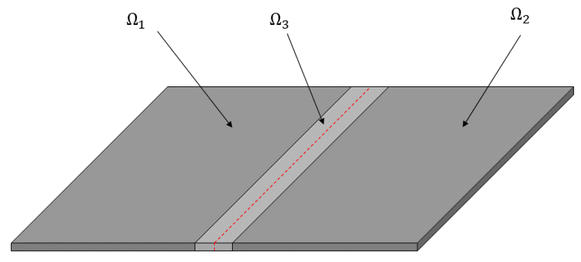
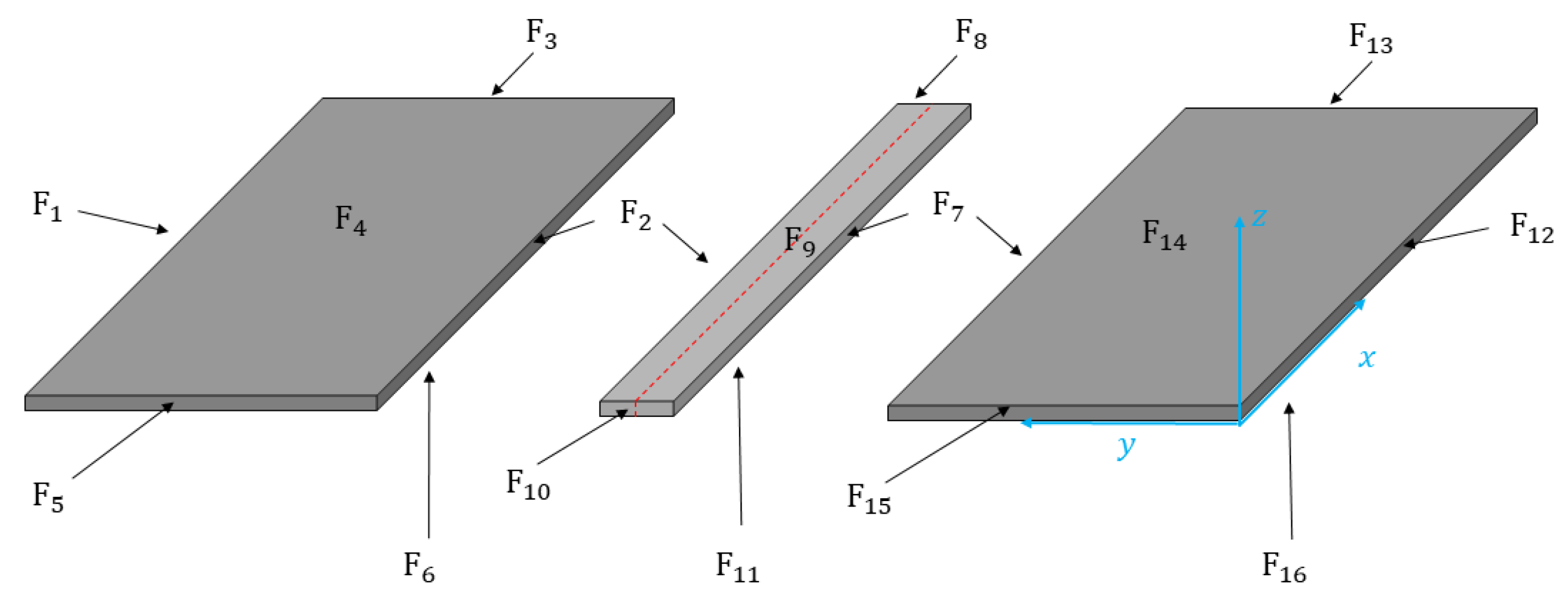
The specimen consists of two Al-Si 5% alloy plates (without surface oxides, which drastically raise the melting temperature), $P_1$ and $P_2$, of equal size (100 mm × 40 mm × 4 mm) (dimensions suggested by IRIS s.r.l.), juxtaposed along the largest dimension such that the respective faces (perfectly smooth) adhere to favor welding. The absence of voids between the plates allows, on one hand, to simulate a better weld quality and, on the other hand, avoids air between the parts to be welded. For our purposes, we divide the domain $\mathrm{\Omega }$ into three subdomains: ${\mathrm{\Omega }}_1$ and ${\mathrm{\Omega }}_2$, which consist of the plates placed side by side net of the $\mathrm{\Omega }$ portion subject to melting and then resolidifying (welding strip); ${\mathrm{\Omega }}_3$ (100 mm × 2 mm × 4 mm) corresponding to the welding strip such that ${\mathrm{\Omega }}_i=P_i\backslash {\mathrm{\Omega }}_3$ with $i=1,2$, in which the heat transfer is modeled according to the melting/resolidification of the material in the interval of temperature $[T_S,T_L]$. Figure 1 shows the partition of $\mathrm{\Omega }$ into $P_1$ and $P_2$ while Figure 2 displays ${\mathrm{\Omega }}_1$ ${\mathrm{\Omega }}_2$ and ${\mathrm{\Omega }}_3$; moreover,

Table 1. Dimensions of ${\mathrm{\Omega }}_1$, ${\mathrm{\Omega }}_2$ and ${\mathrm{\Omega }}_3$.

${\mathbf{\Omega }}_{\mathit{i}}$	Length (mm)	Width (mm)	Thickness (mm)
${\mathrm{\Omega }}_1$	39	100	4
${\mathrm{\Omega }}_2$	39	100	4
${\mathrm{\Omega }}_3$	2	100	4

and

Table 2. Geometric characterizations of ${\mathrm{\Omega }}_1$, ${\mathrm{\Omega }}_2$ and ${\mathrm{\Omega }}_3$.

${\mathbf{\Omega }}_{\mathit{i}}$	Length (mm)	$\stackrel{\circ }{{\mathbf{\Omega }}_{\mathit{i}}}$	Length (mm)
${\mathrm{\Omega }}_1$	$[0,100]\times [0,39]\times [0,4]$	${\stackrel{\circ }{\mathrm{\Omega }}}_1$	$(0,100)\times (0,39)\times (0,4)$
${\mathrm{\Omega }}_2$	$[0,100]\times [41,80]\times [0,4]$	$\stackrel{\circ }{{\mathrm{\Omega }}_2}$	$(0,100)\times (41,80)\times (0,4)$
${\mathrm{\Omega }}_3$	$[0,100]\times [39,41]\times [0,4]$	$\stackrel{\circ }{{\mathrm{\Omega }}_3}$	$(0,100)\times (39,41)\times (0,4)$

highlight the geometry of each ${\mathrm{\Omega }}_i$. Finally, for implementation aims, we label the sixteen faces of $\partial \mathrm{\Omega }$ by $F_i$ ($i=1,\dots ,16$) so that $\partial \mathrm{\Omega }=\left({\displaystyle \bigcup _{i=1}^{16}}{F}_i\right)\backslash \left(F_2\cup F_7\right)$ (see Figure 3), whose dimensions are specified in

Table 3. Geometric characterizations of $\partial {\mathrm{\Omega }}_1$, $\partial {\mathrm{\Omega }}_2$ and $\partial {\mathrm{\Omega }}_3$.

Label	Dimensions	Label	Dimensions
$F_{12}$	$[0,100]\times \left\{0\right\}\times [0,4]$	$F_2$	$[0,100]\times \left\{41\right\}\times [0,4]$
$F_7$	$[0,100]\times \left\{39\right\}\times [0,4]$	$F_1$	$[0,100]\times \left\{80\right\}\times [0,4]$
$F_5$	$\left\{0\right\}\times [41,80]\times [0,4]$	$F_4$	$[0,100]\times [41,80]\times \left\{4\right\}$
$F_3$	$\left\{100\right\}\times [41,80]\times [0,4]$	$F_6$	$[0,100]\times [41,80]\times \left\{0\right\}$
$F_{10}$	$\left\{0\right\}\times [39,41]\times [0,4]$	$F_9$	$[0,100]\times [39,41]\times \left\{4\right\}$
$F_8$	$\left\{100\right\}\times [39,41]\times [0,4]$	$F_{11}$	$[0,100]\times [39,41]\times \left\{0\right\}$
$F_{15}$	$\left\{0\right\}\times [0,39]\times [0,4]$	$F_{14}$	$[0,100]\times [0,39]\times \left\{4\right\}$
$F_{13}$	$\left\{100\right\}\times [0,39]\times [0,4]$	$F_{16}$	$[0,100]\times [0,39]\times \left\{0\right\}$

.

Concerning both ${\mathrm{\Omega }}_1$ and ${\mathrm{\Omega }}_2$, since the laser beam does not pass over them, a model exploiting (1) without a laser heat source is sufficient for recovering $T(\mathbf{x},t)$. Concerning ${\mathrm{\Omega }}_3$, due to the presence of the laser beam, we propose a model where the equation considers the melting/resolidification of the material in its melting range $\Delta T$, in which the replacement heat capacity of the alloy can be formulated according to the known experimental evidence, and from which the volume fraction of the solid state can be easily obtained.

3.2. Domains Not Belonging to the Laser Welding Domain: Model, Initial and Boundary Conditions

Starting from (1), with $Q_l(\mathbf{x},t)=0$ (absence of the laser), and considering thermal conductivity ${\lambda }_i$ independent of the temperature $T_i(\mathbf{x},t)$ that is supposed to be continuous (it makes sense because the thermal conductivity of the AlSi 5% during the laser welding can be considered, in the first approximation, as a constant), we write

$${\mathcal{C}}_S\frac{\partial T_i(\mathbf{x},t)}{\partial t}={\lambda }_i{\nabla }^2{T}_i(\mathbf{x},t),\forall \mathbf{x}\in {\stackrel{\circ }{\mathrm{\Omega }}}_i \text{with} i=1,2,\forall t>0,$$

(16)

to which the following initial conditions can be associated:

$$T_i(\mathbf{x},0)=T_0\forall \mathbf{x}\in {\mathrm{\Omega }}_i \text{with} i=1,2.$$

(17)

Moreover, since the sides of the surfaces are next to the air conduction heat flux $h^{air}[T_{air}-T_i(\mathbf{x},t)]$ and radiation flux $ϵ{\sigma }_B[T_{air}^4-T_i^4(\mathbf{x},t)]$ that occur, where $h_{air}$ is the convection coefficient of air, $ϵ$ is the emissivity and ${\sigma }_B$ the Boltzmann constant. We identify $\widehat{\mathbf{n}}$ the outward unit normal vector to generical faces. Therefore, $\forall \mathbf{x}\in F_j$, $j\in \{1,3,4,5,12,13,14,15\}$ and $\forall t>0$

$${\lambda }_i\frac{\partial T_i(\mathbf{x},t)}{\partial \widehat{\mathbf{n}}}=h^{air}[T_{air}-T_i(\mathbf{x},t)]+ϵ{\sigma }_B[T_{air}^4-T_i^4(\mathbf{x},t)].$$

(18)

Furthermore, for the surfaces in contact with the workbench (faces $F_6$ and $F_{16}$), we introduce the following boundary condition:

$${\lambda }_i\frac{\partial T_i(\mathbf{x},t)}{\partial \widehat{\mathbf{n}}}=h^{bench}[T_{bench}-T_i(\mathbf{x},t)],\forall \mathbf{x}\in F_6\cup F_{16}\forall t>0.$$

(19)

with $h^{bench}$ as the convection coefficient of the workbench. Finally, it is necessary to consider the heat flow coming from ${\mathrm{\Omega }}_3$ toward both ${\mathrm{\Omega }}_1$ and ${\mathrm{\Omega }}_2$; at a certainly higher temperature, the reverse heat flow can be considered negligible because it will not noticeably modify the numerical solution. Considering this heat flow, negligible means a software design “for the benefit of safety” because, strictly speaking, the heat dissipation that goes from the plates towards the welding is miniscule:

$${\lambda }_i\frac{\partial T_i(\mathbf{x},t)}{\partial \widehat{\mathbf{n}}}={\lambda }_3\frac{\partial T_3(\mathbf{x},t)}{\partial \widehat{\mathbf{n}}}\forall \mathbf{x}\in F_2\cup F_7\forall t>0,$$

(20)

Therefore, the model for ${\mathrm{\Omega }}_1$ and ${\mathrm{\Omega }}_2$ can be compactly written as

$$\left\{\begin{array}{c}{\mathcal{C}}_S{\displaystyle \frac{\partial T_i(\mathbf{x},t)}{\partial t}}={\lambda }_i{\nabla }^2{T}_i(\mathbf{x},t),\forall \mathbf{x}\in {\stackrel{\circ }{\mathrm{\Omega }}}_i \mathrm{with} i=1,2\forall t>0\hfill \\ T_i(\mathbf{x},0)=T_0,\forall \mathbf{x}\in {\mathrm{\Omega }}_i \mathrm{with} i=1,2\hfill \\ {\lambda }_i{\displaystyle \frac{\partial T_i(\mathbf{x},t)}{\partial \widehat{\mathbf{n}}}}=h^{air}\left(T_{air}-T_i\right)+ϵ{\sigma }_B\left(T_{air}^4-T_i^4\right),\forall \mathbf{x}\in F_4\cup F_{14}\forall t>0,\hfill \\ {\lambda }_i{\displaystyle \frac{\partial T_i(\mathbf{x},t)}{\partial \widehat{\mathbf{n}}}}=h^{air}\left(T_{air}-T_i\right)+h^{bench}\left(T_{bench}-T_i\right),\forall \mathbf{x}\in F_6\cup F_{16}\forall t>0,\hfill \\ {\lambda }_i{\displaystyle \frac{\partial T_i(\mathbf{x},t)}{\partial \widehat{\mathbf{n}}}}=h^{air}\left(T_{air}-T_i\right),\forall \mathbf{x}\in F_1\cup F_3\cup F_5\cup F_{12}\cup F_{13}\cup F_{15}\forall t>0,\hfill \\ {\lambda }_i{\displaystyle \frac{\partial T_i(\mathbf{x},t)}{\partial \widehat{\mathbf{n}}}}={\lambda }_3{\displaystyle \frac{\partial T_3(\mathbf{x},t)}{\partial \widehat{\mathbf{n}}}},\forall \mathbf{x}\in F_2\cup F_7\forall t>0.\hfill \end{array}\right.$$

(21)

3.3. Laser Welding Domain: The Model

When the laser beam flows on the plates, starting from $T_0$, the temperature $T(\mathbf{x},t)$ increases, raising the melted material, obtaining the following phase transitions:

$$solid\to \underset{intermediate}{\underbrace{solid+liquid}}\to liquid.$$

Furthermore, the laser beam, moving again, melts material further, while the previously melted material, due to the lowering of $T(\mathbf{x},t)$, resolidifies as follows:

$$liquid\to \underset{intermediate}{\underbrace{solid+liquid}}\to solid.$$

To model this process, we start from [25] in which melting and resolidification processes for a metallurgical problem were considered at a temperature interval $\Delta T$. Then, in our case, Equation (6) is valid, to whose right-hand side we add $Q_l^{\left(v\right)}(\mathbf{x},t)$, which models the volumetric moving laser heat source:

$$\mathcal{C}\left(T_3(\mathbf{x},t)\right)\frac{\partial T_3(\mathbf{x},t)}{\partial t}={\lambda }_3{\nabla }^2{T}_3(\mathbf{x},t))+Q_l^{\left(v\right)}(\mathbf{x},t),\forall \mathbf{x}\in {\stackrel{\circ }{\mathrm{\Omega }}}_3\forall t>0,$$

(22)

with the following initial condition:

$$T_3(\mathbf{x},0)=T_0\forall \mathbf{x}\in {\mathrm{\Omega }}_3.$$

(23)

Concerning the boundary conditions, a first Robin condition concerns the heat flow, which flows from ${\mathrm{\Omega }}_3$ towards the workbench (face $F_{11}$):

$${\lambda }_3\frac{\partial T_3(\mathbf{x},t)}{\partial \widehat{\mathbf{n}}}=h^{bench}[T_{bench}-T_3(\mathbf{x},t)]\forall \mathbf{x}\in F_{11}\forall t>0.$$

(24)

Furthermore, the upper side (face $F_9$) is in contact with the air, so the following Cauchy–Stefan–Boltzmann boundary condition makes sense:

$$\begin{array}{cc}\hfill {\lambda }_3\frac{\partial T_3(\mathbf{x},t)}{\partial \widehat{\mathbf{n}}}=& h^{air}[T_{air}-T_3(\mathbf{x},t)]+ϵk_B[T_{air}^4-T_3^4(\mathbf{x},t)]+\hfill \\ \hfill & +Q_l^{\left(s\right)}(\mathbf{x},t)\forall \mathbf{x}\in F_9\forall t>0,\hfill \end{array}$$

(25)

in which the contribution due to irradiation is present ($Q_l^{\left(s\right)}(\mathbf{x},t)$, laser beam heat source). Finally, lateral surfaces of ${\mathrm{\Omega }}_3$ in contact with the internal lateral surfaces of ${\mathrm{\Omega }}_1$ and ${\mathrm{\Omega }}_2$ are only affected by conduction flows; therefore,

$${\lambda }_3\frac{\partial T_3(\mathbf{x},t)}{\partial \widehat{\mathbf{n}}}={\lambda }_i\frac{\partial T_i(\mathbf{x},t)}{\partial \widehat{\mathbf{n}}},\forall \mathbf{x}\in F_2\cup F_7\forall t>0.$$

(26)

So, the model for ${\mathrm{\Omega }}_3$ assumes the following compact form:

$$\left\{\begin{array}{c}\mathcal{C}\left(T_3(\mathbf{x},t)\right){\displaystyle \frac{\partial T_3(\mathbf{x},t)}{\partial t}}={\lambda }_3{\nabla }^2{T}_3(\mathbf{x},t)+Q_l^{\left(v\right)}(\mathbf{x},t),\forall \mathbf{x}\in {\stackrel{\circ }{\mathrm{\Omega }}}_3\forall t>0\hfill \\ T_3(\mathbf{x},0)=T_0,\forall \mathbf{x}\in {\mathrm{\Omega }}_3\hfill \\ {\lambda }_3{\displaystyle \frac{\partial T_3(\mathbf{x},t)}{\partial \widehat{\mathbf{n}}}}=Q_l^{\left(s\right)}(\mathbf{x},t)+\hfill \\ +h^{air}\left(T_{air}-T_3\right)+ϵ{\sigma }_B\left(T_{air}^4-T_3^4\right),\forall \mathbf{x}\in F_9\forall t>0,\hfill \\ {\lambda }_3{\displaystyle \frac{\partial T_3(\mathbf{x},t)}{\partial \widehat{\mathbf{n}}}}=h^{air}\left(T_{air}-T_3\right)+h^{bench}\left(T_{bench}-T_3\right),\forall \mathbf{x}\in F_{11}\forall t>0,\hfill \\ {\lambda }_3{\displaystyle \frac{\partial T_3(\mathbf{x},t)}{\partial \widehat{\mathbf{n}}}}=h^{air}\left(T_{air}-T_3\right),\forall \mathbf{x}\in F_8\cup F_{10}\forall t>0,\hfill \\ {\lambda }_3{\displaystyle \frac{\partial T_3(\mathbf{x},t)}{\partial \widehat{\mathbf{n}}}}={\lambda }_i{\displaystyle \frac{\partial T_i(\mathbf{x},t)}{\partial \widehat{\mathbf{n}}}},\forall \mathbf{x}\in F_2\cup F_7\forall t>0.\hfill \end{array}\right.$$

(27)

3.4. Full Model in the Domain

Finally, for $\mathrm{\Omega }$, the model is compactly written as

$$\left\{\begin{array}{c}\mu {\displaystyle \frac{\partial T(\mathbf{x},t)}{\partial t}}=\lambda {\nabla }^{2}T(\mathbf{x},t)+\eta Q_l^{\left(v\right)}(\mathbf{x},t),\forall \mathbf{x}\in \stackrel{\circ }{\mathrm{\Omega }}\forall t>0\hfill \\ T(\mathbf{x},0)=T_0,\forall \mathbf{x}\in \mathrm{\Omega }\hfill \\ \lambda {\displaystyle \frac{\partial T(\mathbf{x},t)}{\partial \widehat{\mathbf{n}}}}=\eta Q_l^{\left(s\right)}(\mathbf{x},t)+h^{air}\left(T_{air}-T\right)+ϵ{\sigma }_B\left(T_{air}^4-T^4\right),\hfill \\ \forall \mathbf{x}\in F_4\cup F_9\cup F_{14}\forall t>0,\hfill \\ \lambda {\displaystyle \frac{\partial T(\mathbf{x},t)}{\partial \widehat{\mathbf{n}}}}=h^{air}\left(T_{air}-T\right)+h^{bench}\left(T_{bench}-T\right),\hfill \\ \forall \mathbf{x}\in F_6\cup F_{11}\cup F_{16}\forall t>0,\hfill \\ \lambda {\displaystyle \frac{\partial T(\mathbf{x},t)}{\partial \widehat{\mathbf{n}}}}=h^{air}\left(T_{air}-T\right),\hfill \\ \forall \mathbf{x}\in F_1\cup F_3\cup F_5\cup F_8\cup F_{10}\cup F_{12}\cup F_{13}\cup F_{15}\forall t>0,\hfill \end{array}\right.$$

(28)

compactly assumes the form

$$\left\{\begin{array}{c}\mu {\displaystyle \frac{\partial T(\mathbf{x},t)}{\partial t}}=\lambda {\nabla }^{2}T(\mathbf{x},t)+\eta Q_l^{\left(v\right)}(\mathbf{x},t),\forall \mathbf{x}\in \stackrel{\circ }{\mathrm{\Omega }}\forall t>0\hfill \\ T(\mathbf{x},0)=T_0,\forall \mathbf{x}\in \mathrm{\Omega }\hfill \\ \lambda {\displaystyle \frac{\partial T(\mathbf{x},t)}{\partial \widehat{\mathbf{n}}}}+h^{air}\left(T-T_{air}\right)+\beta h^{bench}\left(T-T_{bench}\right)+\alpha ϵ{\sigma }_B\left(T^4-T_{air}^4\right)=\hfill \\ =\eta Q_l^{\left(s\right)}(\mathbf{x},t),\forall \mathbf{x}\in \partial \mathrm{\Omega }\forall t>0.\hfill \end{array}\right.$$

(29)

where

$$T(\mathbf{x},t)=\left\{\begin{array}{c}{T}_1(\mathbf{x},t)\mathrm{if}\mathbf{x}\in {\mathrm{\Omega }}_1,\hfill \\ T_2(\mathbf{x},t)\mathrm{if}\mathbf{x}\in {\mathrm{\Omega }}_2,\hfill \\ T_3(\mathbf{x},t)\mathrm{if}\mathbf{x}\in {\mathrm{\Omega }}_3,\hfill \end{array}\right.$$

(30)

$$\mu =\left\{\begin{array}{c}{\mathcal{C}}_S\mathrm{if}\mathbf{x}\in {\mathrm{\Omega }}_1\cup {\mathrm{\Omega }}_2,\hfill \\ \mathcal{C}\left(T\right)\mathrm{if}\mathbf{x}\in {\mathrm{\Omega }}_3,\hfill \end{array}\right.$$

(31)

$$\lambda =\left\{\begin{array}{c}{\lambda }_1\mathrm{if}\mathbf{x}\in {\mathrm{\Omega }}_1,\hfill \\ {\lambda }_2\mathrm{if}\mathbf{x}\in {\mathrm{\Omega }}_2,\hfill \\ {\lambda }_3\mathrm{if}\mathbf{x}\in {\mathrm{\Omega }}_3,\hfill \end{array}\right.$$

(32)

$$\eta =\left\{\begin{array}{c}0\mathrm{if}\mathbf{x}\in {\mathrm{\Omega }}_1\cup {\mathrm{\Omega }}_2,\hfill \\ 1\mathrm{if}\mathbf{x}\in {\mathrm{\Omega }}_3,\hfill \end{array}\right.$$

(33)

$$\alpha =\left\{\begin{array}{c}1\mathrm{if}\mathbf{x}\in F_6\cup F_{16}\cup F_{11},\hfill \\ 0\mathrm{if}\mathbf{x}\in \partial \mathrm{\Omega }\backslash (F_6\cup F_{16}\cup F_{11}),\hfill \end{array}\right.$$

(34)

$$\beta =\left\{\begin{array}{c}1\mathrm{if}\mathbf{x}\in F_4\cup F_{14}\cup F_9,\hfill \\ 0\mathrm{if}\mathbf{x}\in \partial \mathrm{\Omega }\backslash (F_4\cup F_{14}\cup F_9).\hfill \end{array}\right.$$

(35)

The model simulates the welding process of 5% Al-Si alloy plates, which are widely used in industry, without adding any extra material. This is critical, as it eliminates unwanted thickening and adheres to regulatory standards. Even if the collaboration with IRIS s.r.l. required the use of 5% Al-Si alloy, the model can obtain results for other materials, which, for their laser welding, do not require extra material.

3.5. Realistic Formulations for Both Volumetric and Superficial Laser Heat Sources

To recover $T(\mathbf{x},t)$, it is necessary to define precisely the shape of the “melting hole” and the subsequent solidification scheme. Then, according to the final mechanical properties of the welding, we should mathematically formalize both $Q_l^{\left(v\right)}(\mathbf{x},t)$ and $Q_l^{\left(s\right)}(\mathbf{x},t)$.

3.5.1. Classical Gaussian Laser Heat Source

To model the moving heat source, as a first approach, we use the established volumetric and superficial Gaussian formulation [24]:

$$\begin{array}{cc}\hfill & Q_l^{\left(v\right)}(\mathbf{x},t)=\frac{R_f{I}_0}{r_U}{e}^{-{\displaystyle \frac{{(x-x_0)}^2+{(y-y_0)}^2+{(z-z_0)}^2}{r_U^2}}},\hfill \\ \hfill & Q_l^{\left(s\right)}(\mathbf{x},t)=R_f{I}_0{e}^{-{\displaystyle \frac{{(x-x_0)}^2+{(y-y_0)}^2}{r_U^2}}},\hfill \end{array}$$

(36)

displayed in Figure 4, where $(x_0,y_0,z_0)=(vt,y_0,z_0)$ are the coordinates of the point where the laser beam starts, v denoting the laser speed, $r_U$ the laser radius, $I_0$ the laser intensity (which contributes to give the laser power), and $R_f$ the reflexivity. It basically just means that on the surface that it is interacting with, they define a heat flux proportional to a Gaussian distribution.

3.5.2. Conical Laser Heat Source

As a term of comparison, we will also use the conical laser heat source (see Figure 5) deriving from a Gaussian heat distribution. This allows the following formulations to be used [24]:

$$\begin{array}{cc}\hfill & Q_l^{\left(v\right)}(\mathbf{x},t)=\frac{R_f{I}_0}{r_U}{e}^{-{\displaystyle \frac{{(x-vt)}^2+{(y-y_0)}^2+{(z-z_0)}^2}{r{\left(z\right)}^2}}},\hfill \\ \hfill & Q_l^{\left(s\right)}(\mathbf{x},t)=R_f{I}_0{e}^{-{\displaystyle \frac{{(x-vt)}^2+{(y-y_0)}^2}{r_U^2}}},\hfill \end{array}$$

(37)

where $r\left(z\right)$, representing the action radius of the laser on z, is formulable as

$$r\left(z\right)=r_U-(r_U-r_L)·{\displaystyle \frac{z_U-z}{z_U-z_L}},$$

(38)

in which $r_U$ and $r_L$ represent the radius on $z=z_U$ (upper) and $z=z_L$ (lower), respectively.

3.5.3. Ellipsoid Laser Heat Source

As a further term of comparison, we exploit this interesting formulation, depicted in Figure 6, formulated as [28]

$$\begin{array}{cc}\hfill & Q_l^{\left(v\right)}(\mathbf{x},t)=R_f{\displaystyle \frac{\sqrt{3}P}{abc\pi \sqrt{\pi }}}·e^{-\left[{\displaystyle \frac{{(x-vt)}^2}{a^2}}+{\displaystyle \frac{{(y-y_0)}^2}{b^2}}+{\displaystyle \frac{{(z-z_0)}^2}{c^2}}\right]},\hfill \\ \hfill & Q_l^{\left(s\right)}(\mathbf{x},t)=R_f{\displaystyle \frac{\sqrt{3}P}{ab\pi \sqrt{\pi }}}·e^{-\left[{\displaystyle \frac{{(x-vt)}^2}{a^2}}+{\displaystyle \frac{{(y-y_0)}^2}{b^2}}\right]},\hfill \end{array}$$

(39)

where a, b, and c are the length, the width, and the depth, respectively [28,29,30].

Remark 1.

The solution $T(\mathbf{x},t)$ of (28) is implicitly linked to $I_0$ which, generating the laser beam, represents the primary cause of distribution of $T(\mathbf{x},t)$ in the plates.

4. The Galerkin-FEM Approach

4.1. Some Remarks on Existence, Uniqueness and Regularity of the Solution

We focus our attention on numerical techniques for solving (28) after verifying that it is a well-posed one. Thus, we recall the following:

Theorem 1

(Miranville-Morosanu). Let $\mathrm{\Omega }\subset {\mathbb{R}}^n$ be a bounded domain, with a $C^2$ boundary $\partial \mathrm{\Omega }$. For a finite time $\tilde{t}>0$, we consider the following nonlinear parabolic second-order PDE boundary value problem [23]:

$$\left\{\begin{array}{c}{\displaystyle \frac{\partial T(\mathbf{x},t)}{\partial t}}=\mathrm{\Phi }\left(T(\mathbf{x},t)\right)\nabla ·(K\left(T(\mathbf{x},t)\right)\nabla T(\mathbf{x},t))+\hfill \\ +\mathrm{\Psi }\left(T(\mathbf{x},t)\right)r^{\left(v\right)}(\mathbf{x},t),\mathit{in}(0,\tilde{t}]\times \mathrm{\Omega },\hfill \\ K\left(T(\mathbf{x},t)\right){\displaystyle \frac{\partial T(\mathbf{x},t)}{\partial \widehat{\mathbf{n}}}}+p_1[T(\mathbf{x},t)-{\theta }_1]+p_2[T(\mathbf{x},t)-{\theta }_2]+\hfill \\ +p_3[T^4(\mathbf{x},t)-{\theta }_3^4]=p_4{r}^{\left(s\right)}(\mathbf{x},t),\mathrm{on}(0,\tilde{t}]\times \partial \mathrm{\Omega },\hfill \\ T(\mathbf{x},0)=T_0\left(\mathbf{x}\right)\mathit{on}\mathrm{\Omega }.\hfill \end{array}\right.$$

(40)

where $\mathrm{\Phi }\left(T\right(\mathbf{x},t\left)\right)$ controls the speed of the diffusion process; $K\left(T\right(\mathbf{x},t\left)\right)$ represents the mobility attached to the solution $T(\mathbf{x},t)$; and $r^{\left(v\right)}(\mathbf{x},t)$ and $r^{\left(s\right)}(\mathbf{x},t)$ are the distributed control and boundary control, respectively. Furthermore, ∇ denotes the gradient, $\widehat{\mathbf{n}}=\widehat{\mathbf{n}}\left(\mathbf{x}\right)$ is the outward unit normal vector to Ω as a point $\mathbf{x}\in \partial \mathrm{\Omega }$ and ${\displaystyle \frac{\partial }{\partial \widehat{\mathbf{n}}}}$ denotes differentiation along $\widehat{\mathbf{n}}$. If the following conditions are satisfied, then problem (40) is well posed:

(1) 

$p_1$, $p_2$, $p_3$, and $p_4$ are non-negative constants;

(2) 

$\mathrm{\Phi }\left(T\right(\mathbf{x},t\left)\right)$ is a positive and bounded real function of class $C^1((0,\tilde{t}]\times \mathrm{\Omega })$ with a bounded derivative;

(3) 

$K\left(T\right(\mathbf{x},t\left)\right)$ assumed to satisfy the following inequality:

$$0<K_m\le K\left(T(\mathbf{x},t)\right)\le K_M,\forall (\mathbf{x},t)\in (0,\tilde{t}]\times \mathrm{\Omega };$$

where $K_m$, $K_M$ are constants;

(4) 

$\mathrm{\Psi }\left(T\right(\mathbf{x},t\left)\right)$ is a positive bounded real function;

(5) 

$r^{\left(v\right)}(\mathbf{x},t)\in L^p((0,\tilde{t}]\times \mathrm{\Omega })$ with $p\ge 2$;

(6) 

$r^{\left(s\right)}(\mathbf{x},t)\in W_p^{1-\frac{1}{2p},2-\frac{1}{p}}((0,\tilde{t}]\times \partial \mathrm{\Omega })$;

(7) 

$T_0\left(\mathbf{x}\right)\in W_{\infty }^{2-\frac{2}{p}}\left(\mathrm{\Omega }\right)$, verifying

$$\begin{array}{c}\hfill K\left(T_0\left(\mathbf{x}\right)\right){\displaystyle \frac{\partial T_0\left(\mathbf{x}\right)}{\partial \widehat{\mathbf{n}}}}+p_1[T_0\left(\mathbf{x}\right)-{\theta }_1]+p_2[T_0\left(\mathbf{x}\right)-{\theta }_2]+p_3[T_0^4\left(\mathbf{x}\right)-{\theta }_3^4]=p_4{r}^{\left(s\right)}(\mathbf{x},0);\end{array}$$

Proof of Theorem 1.

For the proof of this theorem, refer to [23].  □

Remark 2.

It is worth noting that Theorem 1 requires that $\mathrm{\Phi }\left(T\right(\mathbf{x},t\left)\right)$ is a positive real function, bounded, above all, of $C^1((0,\tilde{t}]\times \mathrm{\Omega })$, requiring the continuity of $T(\mathbf{x},t)$.

Theorem 1 can be successfully applied in our laser welding process setting

$$\mathrm{\Phi }\left(T(\mathbf{x},t)\right)={\displaystyle \frac{1}{\mu \left(T\right(\mathbf{x},t\left)\right)}},$$

(41)

$$K\left(T(\mathbf{x},t)\right)=\lambda ,K_m\le K\le K_M,$$

(42)

$$\mathrm{\Psi }\left(T(\mathbf{x},t)\right)={\displaystyle \frac{\eta }{\mu \left(T\right(\mathbf{x},t\left)\right)}},$$

(43)

$$\begin{array}{cc}\hfill & p_1=h^{air},p_2=\beta h^{bench},p_3=\alpha ϵ{\sigma }_B,p_4=\eta ,\hfill \\ \hfill & {\theta }_1=T_{air},{\theta }_2=T_{bench},{\theta }_3=T_{air},\hfill \\ \hfill & r^{\left(v\right)}(\mathbf{x},t)=Q_l^{\left(v\right)}(\mathbf{x},t),r^{\left(s\right)}(\mathbf{x},t)=Q_l^{\left(s\right)}(\mathbf{x},t).\hfill \end{array}$$

(44)

Thus, the non-linear inhomogeneous parabolic model (29) is achieved. It is easy to prove that $Q_l^{\left(v\right)}(\mathbf{x},t)\in L_p((0,\tilde{t}]\times \partial \mathrm{\Omega })$, $Q_l^{\left(s\right)}(\mathbf{x},t)\in W_p^{1-\frac{1}{2p},2-\frac{1}{p}}((0,\tilde{t}]\times \partial \mathrm{\Omega })$. So, Theorem 1 guarantees the well posedness of solutions to the problem (29).

4.2. Galerkin-FEM Basics

According to Section 3.4, we rewrite both the equation and boundary conditions of (28) as follows [31]:

$$\begin{array}{cc}\hfill R_1:& \mu \frac{\partial T(\mathbf{x},t)}{\partial t}-\lambda {\nabla }^{2}T(\mathbf{x},t)-\eta Q_l^{\left(v\right)}(\mathbf{x},t)=0,\hfill \\ \\ \hfill R_2:& \lambda \frac{\partial T(\mathbf{x},t)}{\partial \widehat{\mathbf{n}}}-\beta h^{bench}[T_{bench}-T(\mathbf{x},t)]-h^{air}[T_{air}-T(\mathbf{x},t)]+\hfill \\ \hfill & -\alpha ϵ{\sigma }_B[T_{air}^4-T^4(\mathbf{x},t)]-\eta Q_l^{\left(s\right)}(\mathbf{x},t)=0.\hfill \end{array}$$

(45)

If $w_1$ and $w_2$ are two weight functions, from both (45), we can write

$${\int }_{\mathrm{\Omega }}{w}_1{R}_{1}d\mathrm{\Omega }+{\int }_{\partial \mathrm{\Omega }}{w}_2{R}_{2}d(\partial \mathrm{\Omega })=0,$$

(46)

The first integral in (46) becomes

$$\begin{array}{cc}\hfill {\int }_{\mathrm{\Omega }}{w}_1{R}_{1}d\mathrm{\Omega }=& {\int }_{\mathrm{\Omega }}{w}_1\left(\mu \frac{\partial T(\mathbf{x},t)}{\partial t}\right)d\mathrm{\Omega }+\hfill \\ \hfill & -{\int }_{\mathrm{\Omega }}{w}_1\lambda {\nabla }^{2}T(\mathbf{x},t)d\mathrm{\Omega }-{\int }_{\mathrm{\Omega }}{w}_1\eta Q_l^{\left(v\right)}(\mathbf{x},t)d\mathrm{\Omega }.\hfill \end{array}$$

(47)

Integrating by parts, the second integral of the right side in (47) becomes

$$\begin{array}{c}\hfill {\int }_{\mathrm{\Omega }}{w}_1\lambda {\nabla }^{2}T(\mathbf{x},t)d\mathrm{\Omega }={\int }_{\partial \mathrm{\Omega }}\lambda w_1\frac{\partial T(\mathbf{x},t)}{\partial \widehat{\mathbf{n}}}d(\partial \mathrm{\Omega })-{\int }_{\mathrm{\Omega }}\lambda \nabla w_1·\nabla T(\mathbf{x},t)d\mathrm{\Omega }.\end{array}$$

(48)

Therefore, Equation (47), by means of (48), is writable as

$$\begin{array}{cc}\hfill {\int }_{\mathrm{\Omega }}{w}_1{R}_{1}d\mathrm{\Omega }=& {\int }_{\mathrm{\Omega }}{w}_1\mu \frac{\partial T(\mathbf{x},t)}{\partial t}d\mathrm{\Omega }-{\int }_{\partial \mathrm{\Omega }}\lambda w_1\frac{T(\mathbf{x},t)}{\partial \widehat{\mathbf{n}}}d(\partial \mathrm{\Omega })+\hfill \\ \hfill & +{\int }_{\mathrm{\Omega }}\lambda \nabla w_1·\nabla T(\mathbf{x},t)d\mathrm{\Omega }-{\int }_{\mathrm{\Omega }}{w}_1\eta Q_l^{\left(v\right)}(\mathbf{x},t)d\mathrm{\Omega }=0,\hfill \end{array}$$

(49)

from which

$$\begin{array}{cc}\hfill {\int }_{\partial \mathrm{\Omega }}\lambda w_1\frac{\partial T(\mathbf{x},t)}{\partial \widehat{\mathbf{n}}}d(\partial \mathrm{\Omega })=& {\int }_{\mathrm{\Omega }}{w}_1\left(\mu \frac{\partial T(\mathbf{x},t)}{\partial t}-\eta Q_l^{\left(v\right)}(\mathbf{x},t)\right)d\mathrm{\Omega }+\hfill \\ \hfill & +{\int }_{\mathrm{\Omega }}\lambda \nabla w_1·\nabla T(\mathbf{x},t)d\mathrm{\Omega }.\hfill \end{array}$$

(50)

The second integral in (46), $\forall i\in \{1,2,3\}$ and $\forall j\in \{1,2,\dots ,16\}$, becomes

$$\begin{array}{cc}\hfill {\int }_{\partial \mathrm{\Omega }}{w}_2{R}_{2}d(\partial \mathrm{\Omega })=& {\int }_{\partial \mathrm{\Omega }}{w}_2\{\lambda \frac{\partial T(\mathbf{x},t)}{\partial \widehat{\mathbf{n}}}-\beta h^{bench}[T_{bench}-T(\mathbf{x},t)]+\hfill \\ \hfill & -h^{air}[T_{air}-T(\mathbf{x},t)]-\alpha ϵ{\sigma }_B[T_{air}^4-T^4(\mathbf{x},t)]+\hfill \\ \hfill & -\eta Q_l^{\left(s\right)}(\mathbf{x},t)\}d(\partial \mathrm{\Omega })=0,\hfill \end{array}$$

(51)

from which

$$\begin{array}{cc}\hfill {\int }_{\partial \mathrm{\Omega }}\lambda w_2\frac{\partial T(\mathbf{x},t)}{\partial \widehat{\mathbf{n}}}d(\partial \mathrm{\Omega })=& {\int }_{\partial \mathrm{\Omega }}{w}_2\eta Q_l^{\left(s\right)}(\mathbf{x},t)d(\partial \mathrm{\Omega })+\hfill \\ \hfill & +{\int }_{\partial \mathrm{\Omega }}{w}_2\beta h^{bench}[T_{bench}-T(\mathbf{x},t)]d(\partial \mathrm{\Omega })+\hfill \\ \hfill & +{\int }_{\partial \mathrm{\Omega }}{w}_2{h}^{air}[T_{air}-T(\mathbf{x},t)]d(\partial \mathrm{\Omega })+\hfill \\ \hfill & +{\int }_{\partial \mathrm{\Omega }}{w}_2\alpha ϵ{\sigma }_B[T_{air}^4-T^4(\mathbf{x},t)]d(\partial \mathrm{\Omega }).\hfill \end{array}$$

(52)

For $w_1=w_2=w$, both (50) and (52) have the same left side so that, subtracting side by side, we can write

$$\begin{array}{cc}\hfill & {\int }_{\mathrm{\Omega }}w\left(\mu \frac{\partial T(\mathbf{x},t)}{\partial t}-\eta Q_l^{\left(v\right)}(\mathbf{x},t)\right)d\mathrm{\Omega }+{\int }_{\mathrm{\Omega }}\lambda w\nabla w·\nabla T(\mathbf{x},t)d\mathrm{\Omega }+\hfill \\ \hfill & -{\int }_{\partial \mathrm{\Omega }}w\eta Q_l^{\left(s\right)}(\mathbf{x},t)d(\partial \mathrm{\Omega })-{\int }_{\partial \mathrm{\Omega }}w\beta h^{bench}[T_{bench}-T(\mathbf{x},t)]d(\partial \mathrm{\Omega })+\hfill \\ \hfill & -{\int }_{\partial \mathrm{\Omega }}w{h}^{air}[T_{air}-T(\mathbf{x},t)]d(\partial \mathrm{\Omega })-{\int }_{\partial \mathrm{\Omega }}w\alpha ϵ{\sigma }_B[T_{air}^4-T^4(\mathbf{x},t)]d(\partial \mathrm{\Omega })=0.\hfill \end{array}$$

(53)

We discretize $\mathrm{\Omega }$ into n nodes, on each of which the temperature is indicated with $T_k$ ($k=1,\dots ,n$). If $N_k$ are the shape functions, then

$$T=\sum _{k=1}^n{N}_k{T}_k=N_1{T}_1+N_2{T}_2+\cdots +N_n{T}_n,$$

(54)

$$\begin{array}{cc}\hfill & T=\left[N\right]\left\{T\right\}=\sum _{i=1}^n{N}_i{T}_i,T^4=\left[N\right]\left\{T^4\right\},\frac{\partial T}{\partial t}=\left[N\right]\left\{\dot{T}\right\},\hfill \\ \hfill & \frac{\partial T}{\partial x}=\left[N_x\right]\left\{T\right\},\frac{\partial T}{\partial y}=\left[N_y\right]\left\{T\right\},\frac{\partial T}{\partial z}=\left[N_z\right]\left\{T\right\}.\hfill \end{array}$$

(55)

Assuming that the weight functions are equal to the shape functions, the following makes sense:

$$\frac{\partial w}{\partial x}=\left[N_x\right],\frac{\partial w}{\partial y}=\left[N_y\right],\frac{\partial w}{\partial z}=\left[N_z\right],$$

(56)

so that (53) becomes

$$\begin{array}{cc}\hfill & {\int }_{\mathrm{\Omega }}\mu \left(\left[N\right]\left\{T\right\}\right)\left[N\right]\left\{\dot{T}\right\}d\mathrm{\Omega }+{\int }_{\mathrm{\Omega }}\lambda \left(\left[N_x\right]\left[N_x\right]+\left[N_y\right]\left[N_y\right]+\left[N_z\right]\left[N_z\right]\right)\left\{T\right\}d\mathrm{\Omega }=\hfill \\ \hfill & ={\int }_{\mathrm{\Omega }}\left[N\right]\eta Q_l^{\left(v\right)}(\mathbf{x},t)d\mathrm{\Omega }+{\int }_{\partial \mathrm{\Omega }}\left[N\right]\left\{T^4\right\}d(\partial \mathrm{\Omega })+{\int }_{\partial \mathrm{\Omega }}\eta Q_l^{\left(s\right)}(\mathbf{x},t)d(\partial \mathrm{\Omega })+\hfill \\ \hfill & +{\int }_{\partial \mathrm{\Omega }}\left[N\right]\beta h^{bench}{T}_{bench}d(\partial \mathrm{\Omega })+{\int }_{\partial \mathrm{\Omega }}\left[N\right]h^{air}{T}_{air}d(\partial \mathrm{\Omega })+\hfill \\ \hfill & +{\int }_{\partial \mathrm{\Omega }}\left[N\right]\alpha ϵ{\sigma }_B{T}_{air}^{4}d(\partial \mathrm{\Omega })-{\int }_{\partial \mathrm{\Omega }}\left[N\right]\beta h^{bench}\left[N\right]\left\{T\right\}d(\partial \mathrm{\Omega })+\hfill \\ \hfill & -{\int }_{\partial \mathrm{\Omega }}\left[N\right]h^{air}\left[N\right]\left\{T\right\}d(\partial \mathrm{\Omega })-{\int }_{\partial \mathrm{\Omega }}\left[N\right]\alpha ϵ{\sigma }_B\left[N\right]\left\{T^4\right\}d(\partial \mathrm{\Omega }).\hfill \end{array}$$

(57)

Therefore, indicating by

$$\begin{array}{cc}\hfill =& {\int }_{\mathrm{\Omega }}\mu \left[N\right]d\mathrm{\Omega },\hfill \\ \hfill \left[\tilde{Y}\right]=& \left[K\right]+\left[Y\right],\hfill \\ \hfill \left[K\right]=& {\int }_{\mathrm{\Omega }}\lambda \left(\left[N_x\right]\left[N_x\right]+\left[N_y\right]\left[N_y\right]+\left[N_z\right]\left[N_z\right]\right)d\mathrm{\Omega },\hfill \\ \hfill \left[Y\right]=& {\int }_{\partial \mathrm{\Omega }}\left(\beta h^{bench}\left[N\right]\left[N\right]+h^{air}\left[N\right]\left[N\right]d(\partial \mathrm{\Omega })\right),\hfill \\ \hfill \left[H\right]=& {\int }_{\partial \mathrm{\Omega }}\alpha ϵ{\sigma }_B\left[N\right]\left[N\right]d(\partial \mathrm{\Omega }),\hfill \\ \hfill \left\{F\right\}=& {\int }_{\mathrm{\Omega }}\left[N\right]\eta Q_l^{\left(v\right)}(\mathbf{x},t)d\mathrm{\Omega }+{\int }_{\partial \mathrm{\Omega }}\eta Q_l^{\left(s\right)}(\mathbf{x},t)d(\partial \mathrm{\Omega })+{\int }_{\partial \mathrm{\Omega }}\left(\beta h^{bench}{T}_{bench}\left[N\right]+\right.\hfill \\ \hfill & +\left.h^{air}{T}_{air}\left[N\right]+\alpha ϵ{\sigma }_B{T}_{air}^4\left[N\right]\right)d(\partial \mathrm{\Omega }).\hfill \end{array}$$

(58)

(57) is writable as

$$\left[Z\right]\left\{\dot{T}\right\}+\left[\tilde{K}\right]\left\{T\right\}+\left[H\right]\left\{T^4\right\}=\left\{F\right\},$$

(59)

whose integrals are computed by the Crank–Nicholson procedure. The FEM approach, according to (59), was numerically implemented on an Intel Core 2 CPU 1.45 GHz machine and MatLab R2022 PDE tool, testing them on different kinds of laser sources as described in Section 3.5.

5. Results of Computations

Here, the results obtained using the laser heat source as detailed above are presented and discussed. The physical parameters of the alloy Al-Si $5\%$, kindly provided by IRIS s.r.l., are listed in

Table 4. Physical parameters of Al-Si $5\%$ alloy.

Parameter	Value	Unit
${\mathcal{C}}_S$	$2.943\times {10}^6$	J/(m3 K)
${\mathcal{C}}_L$	$3.07\times {10}^6$	J/(m3 K)
$\lambda$	290	W/(m K)
$L_v$	$990.6\times {10}^6$	J/(m3)
$T_S$	$850.15$	K
$T_L$	$923.15$	K
$ϵ$	$0.8$

, and the laser physical parameters related to a typical welding process for alloy Al-Si $5\%$ are listed in

Table 5. Laser parameters.

Parameter	Significance	Value	Unit
v	velocity	40	mm/s
P	power	2400	W
$r_U$	radius	$1.5$	mm
$R_f$	reflexivity	$0.9$
$I_0$	intensity	340	W/mm2

(the laser intensity is computed by $I_0=P/\pi r_U^2$).

Furthermore, we set ${\sigma }_B=1.35\times {10}^{-23}J/K$, $T_0=T_{air}=T_{bench}=298$ K (typical environmental temperature in welding forge [32,33,34]), $h^{air}=15\times {10}^{-6}$ W/(mm² K), and $h^{bench}=20h^{air}$ (as experimentally suggested from metallurgical experiments [35,36,37,38,39,40] to guarantee the correct penetration without favoring the thermal degradation of the alloy structure, and it is such that it produces significant effects even at depth).

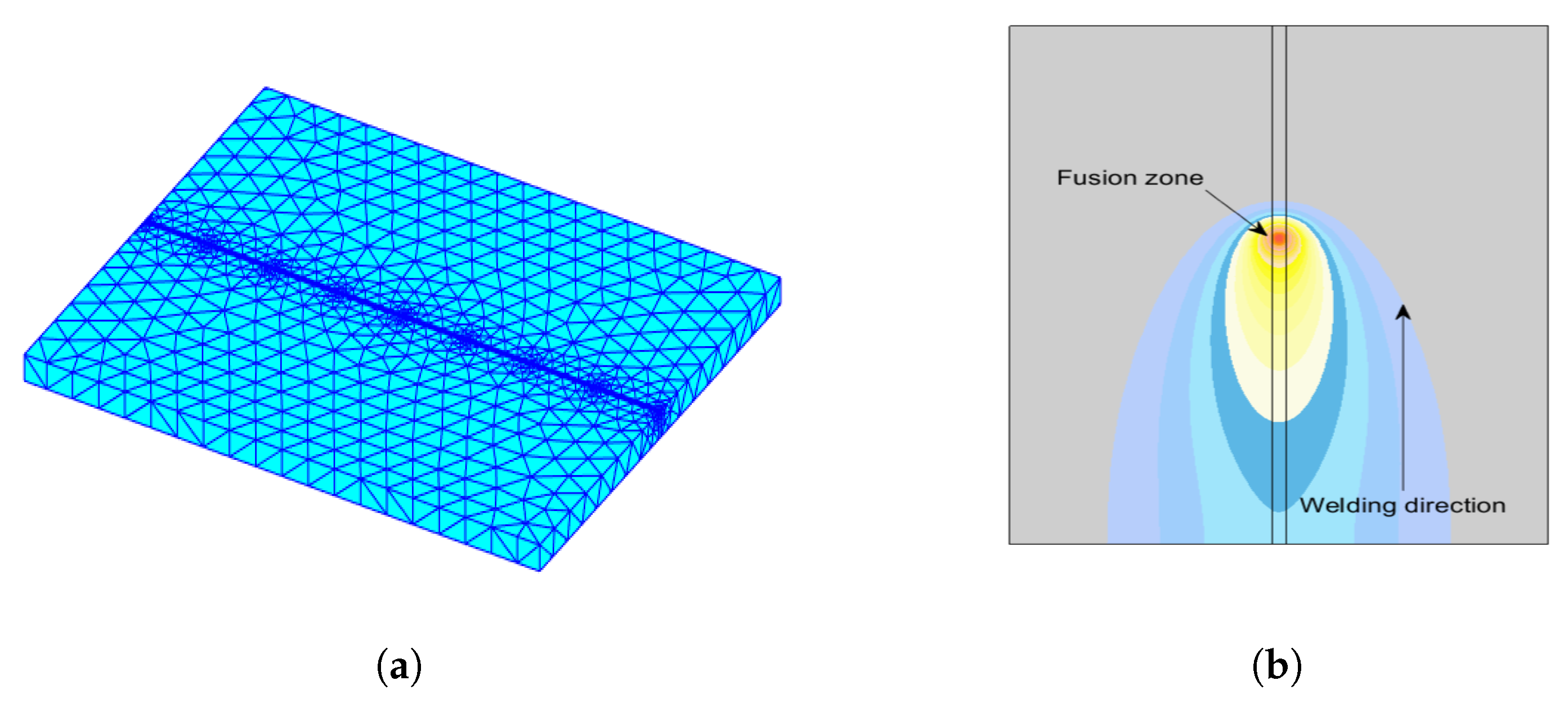
Galerkin-FEM procedure applied to (28), described above and implemented in MatLab R2022 PDE Tool, optimizes a mesh with tetrahedral elements. To obtain reliable and superimposable results with experimental evidence, $\mathrm{\Omega }$ was discretized by a mesh with 3500 finite elements (4522 nodes, 3924 edges), which thicken in the vicinity and especially in correspondence of ${\mathrm{\Omega }}_3$ (welding area), where the melting process takes place (Figure 7a). Moreover, the mesh refinement at ${\mathrm{\Omega }}_3$ was also slightly extended in ${\mathrm{\Omega }}_1$ and ${\mathrm{\Omega }}_2$ to perform the temperature reduction in passing from the welding area to the remaining part of $\mathrm{\Omega }$. Furthermore, the quality of the mesh was confirmed by computing the indices presented in Section 5.1, whose values obtained fall within the respective ranges of admissible values for good-quality meshes.

The lasting of the considered welding process is $2.5$ s, as is the usual practice for the laser welding of plates of dimensions compatible with those fixed in this work [36] (see Figure 7b, where the red point represents the impact point of the laser beam). Once the laser has melted the material, advancing further along the joining line of the plates, the molten material resolidifies, thanks to the significant drop in temperature (blue area, see Figure 7b).

5.1. Mesh Creation

We create the mesh ($\overline{T}=\left\{E_k\right\}$), where $E_k$ is the generic finite element and such that $E_k\cap E_{k^{\prime }}=\varnothing$, $k\ne k^{\prime },\forall k\ne k^{\prime }$ (is either empty or consists of exactly one node or of one edge), obtained with triangulation techniques to obtain tetrahedral finite elements. We discretized $\mathrm{\Omega }$ in order that ($\mathrm{\Omega }={\cup }_{k=1}^{N_{\overline{T}}}{E}_k$), with $N_{\overline{T}}=\left|\overline{T}\right|$. Moreover, the size of the mesh h, $h\left(E_k\right)$ is quantifiable as [31] $h\left(E_k\right)={sup}_{x,y\in E_k}\parallel x-y\parallel$ so that $h={max}_{E_k\in \overline{T}}\left(E_k\right)$. Particularly, the volume of each $E_k$, indicated by $V_k$, is computable as

$$V_k=\frac{1}{6}\left|\begin{array}{ccc}{x}_2-x_1& x_3-x_1& x_4-x_1\\ y_2-y_1& y_3-y_1& y_4-y_1\\ z_2-z_1& z_3-z_1& z_4-z_1\end{array}\right|$$

(60)

where $x_i,y_i,z_i$ are the coordinates of the vertices $P_i$ of $E_k$. Moreover, for each triangle of $E_k$, the surface is

$$S_k=0.5\left|\begin{array}{cc}{x}_2-x_1& x_3-x_1\\ y_2-y_1& y_3-y_1\end{array}\right|.$$

(61)

Therefore, a face of $E_k$ is an ordered triad (allowing all possible combinations), while the edges are considered, not as elements of the faces but as separate entities, and are implicitly defined in terms of ordered pairs of vertices. To each $E_k$, we associate the sphere circumscribed at its vertices whose radius $C_k$ and its center can be obtained by solving the equation

$$C_k=\left|\begin{array}{cccc}{l}_1^2-l^2& l_2^2-l_1^2& l_3^2-l_1^2& l_4^2-l_1^2\\ x_1-x& x_2-x_1& x_3-x_1& x_4-x_1\\ y_1-y& y_2-y_1& y_3-y_1& y_4-y_1\\ z_1-z& z_2-z_1& z_3-z_1& z_4-z_1\end{array}\right|$$

(62)

where $l^2=x^2+y^2+z^2$ and $l_i^2=x_i^2+y_i^2+z_i^2$ ($i=1,\dots ,4$), or solving a system of linear equation for achieving the center. As in two dimensions, there is a formula that allows you to calculate the radius and that allows you to avoid calculating $C_k$:

$$r_k={\left(24V_k\right)}^{-1}{\left((m+n+s)(m+n-s)(n+s-m)(m-n+s)\right)}^{0.5}$$

(63)

where m, n and s are the products of the lengths of two opposite edges. Finally, the radius of the inscribed sphere can be evaluated as

$${\gamma }_k=3V_k{(S_1+S_2+S_3+S_4)}^{-1},$$

(64)

where $S_i$ is the surface of the triangle i of $E_k$. Since the simulations require rather long execution times, we previously evaluated the quality of the meshes obtained. In particular, three well-established quality indices were exploited: aspect ratio, Jacobian ratio, maximum corner angle and skewness [31]. For each triangular element, the aspect ratio values obtained, which are an index that guarantees good numerical accuracy if all sides of an element are of equal length, are all very close to 1. In parallel, for each tetrahedron, the value obtained for the Jacobian ratio, which quantifies whether each average node is positioned in the center with respect to two adjacent nodes, is also very close to 1. The maximum angles between two sides of each element were also evaluated, obtaining values much smaller than $2\pi$ rad; this cautions us against the possible degradation of performance. Finally, the asymmetries were also evaluated, which resulted to be very close to the zero value. These obtained values highlight the excellent quality of the constructed meshes. Furthermore, the ToolBox uses automatic generation techniques of high-quality meshes in relation to the type of problem to be solved. Also, using the “MeshQuality” ToolBox further controlled the quality of the mesh. Finally, during the simulation campaign, we compared the results obtained with similar cases known in the literature.

5.2. Exploiting Classical Gaussian Laser Heat Source

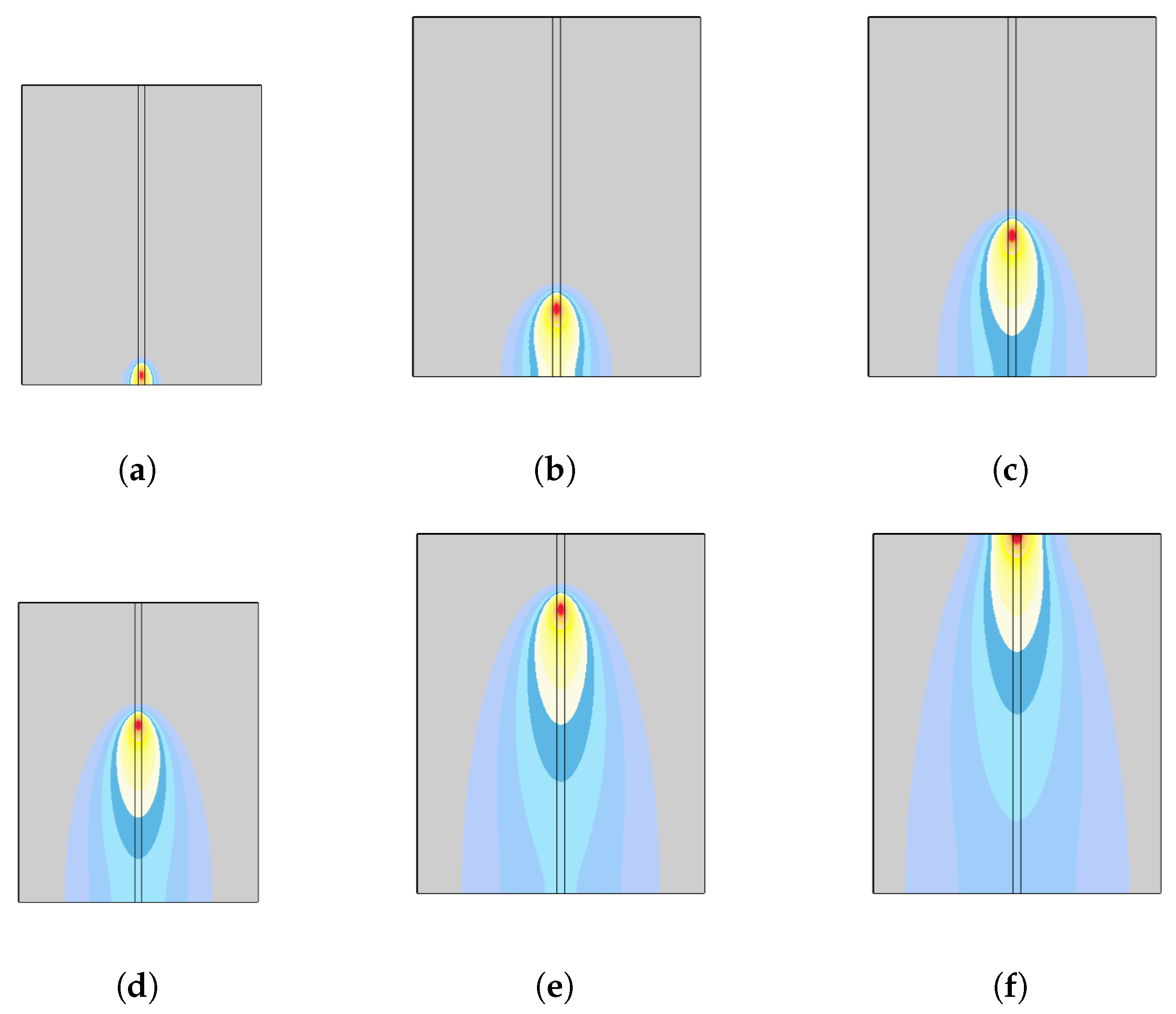
As already specified, the duration of the welding process is equal to $2.5$ s, in accordance with the executive practice of laser welding for plates, whose dimensions are compatible with those specified in this [36] paper. Figure 8 displays the welding process implemented in MatLab; once the material has melted, the laser advances along the joint line of the slabs, melting further material, while the previously melted material solidifies as the temperature drops drastically. Figure 9a and Figure 10a, relating to the final point of the weld, offer greater evidence of this phenomenon, emphasizing that, already in the numerical simulation phase, (28) models the underlying component of the proposed approach. As highlighted in Figure 7a, the mesh is not a capillary over $\mathrm{\Omega }$ but only over ${\mathrm{\Omega }}_3$ and its immediate vicinity because (28) does not consider any delay times for the distribution of $T(\mathbf{x},t)$ during the passage of the laser beam. Therefore, considering this distribution throughout $\mathrm{\Omega }$ to be instantaneous, the cooling in both ${\mathrm{\Omega }}_1$ and ${\mathrm{\Omega }}_2$ is immediate, also considering that the thermal conduction between the plates and the workbench is also taken into account.

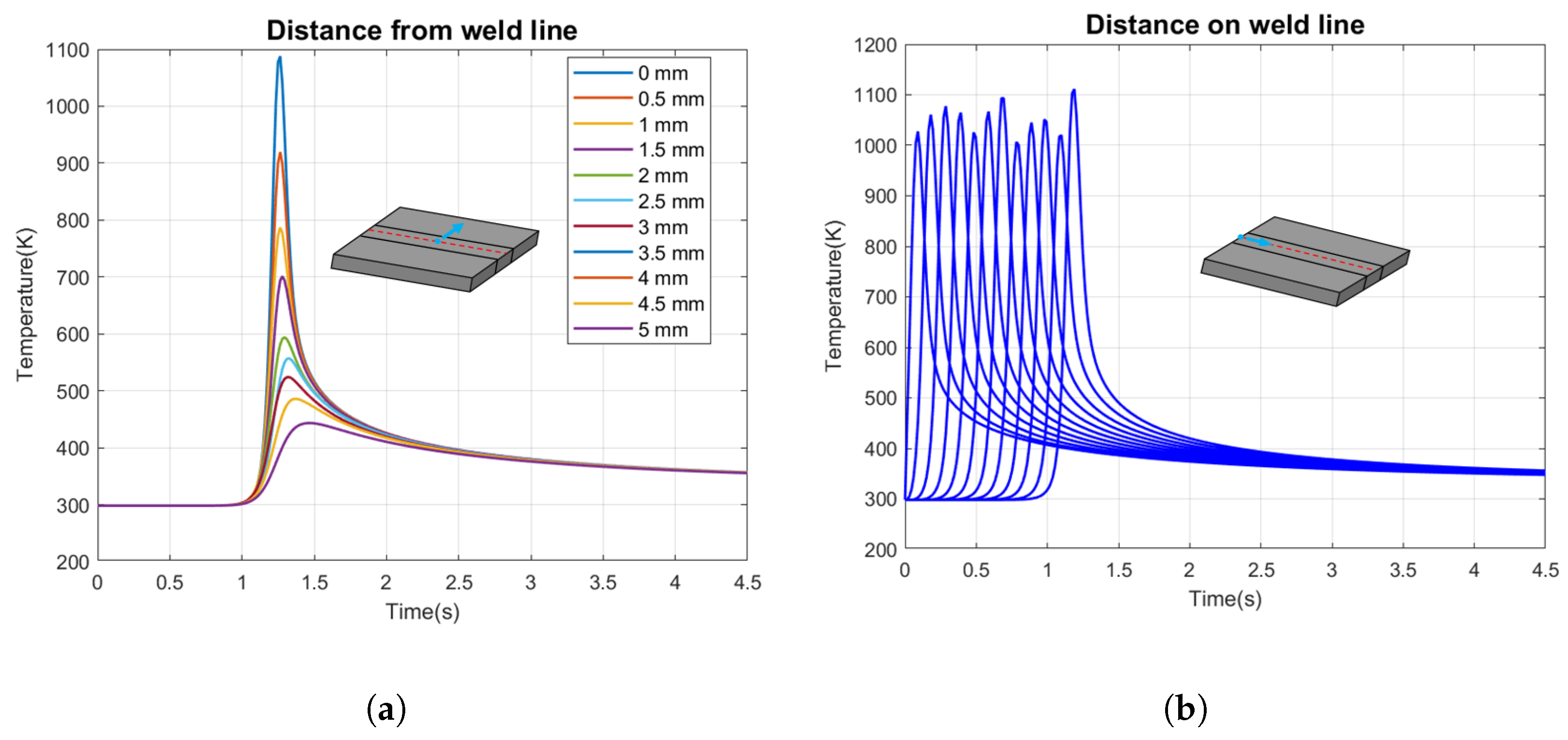
Both Figure 11a,b depict this aspect because they show the distribution of $T(\mathbf{x},t)$ both in the initial point and in five different points of the welding wire, from which it can be seen that once the temperature peak has been reached, as the laser beam advances, the cooling is locally evident. Furthermore, the final point of the welding path is affected both by the presence of the laser beam and by the conduction of the other points where the welding has already taken place. In fact, the peaks increase as the weld progresses toward the endpoint. However, we observe that this remark does not affect the quality of the proposed model because, regardless of any delay times in the distribution of $T(\mathbf{x},t)$, ${\mathrm{\Omega }}_3$ remains the most thermally stressed area, where after the laser welding process, the mechanical properties are checked. In confirmation of the above, the thermal cycles were obtained transversally to the welding line (in correspondence with its midpoint), by which it is once again highlighted how, moving away from the welding line, the cooling of the plates is drastic (see Figure 12a). On the other hand, moving along the welding line, the thermal cycles show behaviors that are qualitatively/quantitatively similar to each other (see Figure 12b). Particularly, during the welding process, the temperature peaks are well above the melting range of the alloy as required by the welding execution practice to guarantee the melting of the material along the entire depth of the plates.

5.3. Exploiting Conical 3D Laser Heat Source

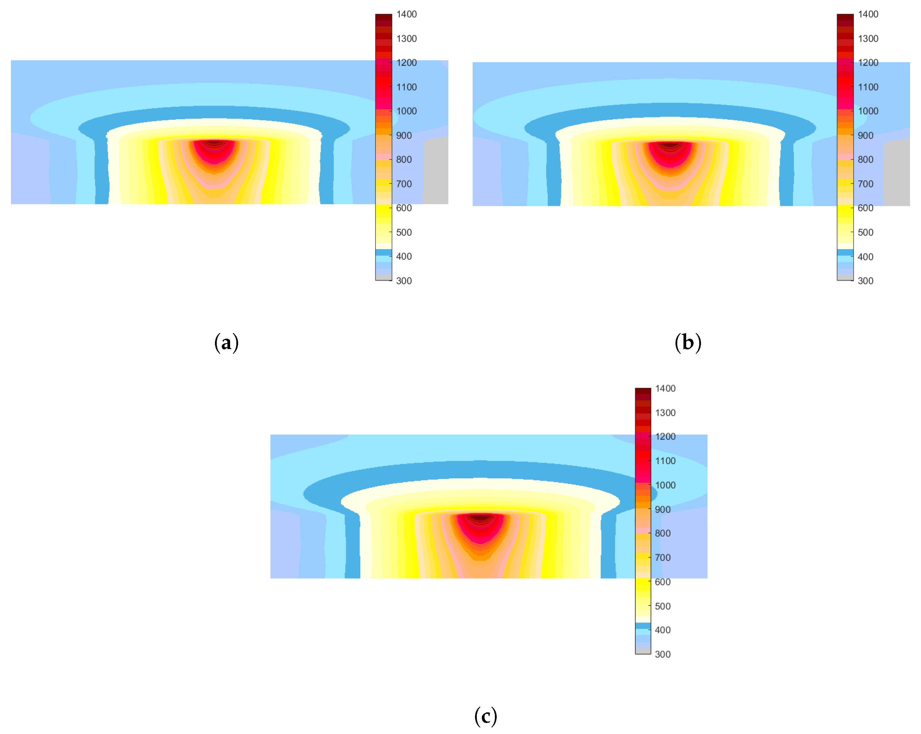
Here, we exploit the same mesh used for the simulations with the classical Gaussian 3D laser heat source because further refinements significantly increase the computational complexity without appreciable performance improvements. We set all parameters, as in Section 5.2. Moreover, here $z_U=4$ mm and $z_L=0$ mm, as often happens in many aluminum alloy plate welding processes. Therefore, the $T(\mathbf{x},t)$ distribution in $\mathrm{\Omega }$ as highlighted in Figure 9b and Figure 10b (when the laser beam reaches the final position of the welding path) simulates a laser welding of the same duration as the one simulated in Section 5.2. Further in this case, in ${\mathrm{\Omega }}_3$, $T(\mathbf{x},t)$, throughout the welding process, settles on values, ensuring the fusion of the aluminum even in depth, although the temperatures reached are higher than when a classical Gaussian 3D laser head source is considered, risking carrying out a melting and resolidification process that does not meet the required quality standards. As regards the thermal cycles both transversely and longitudinally of the welding line, they appear qualitatively superimposable to those obtained in Figure 12a,b. Thus, (28) does not consider any thermal losses (as well as any time lag that slows down the temperature distribution), and the conical 3D laser head source is not suitable to model the laser beam because the real $T(\mathbf{x},t)$ in ${\mathrm{\Omega }}_3$, being oversized, cannot guarantee the total melting of the alloy without compromising the internal structure of the material. This phenomenon is more evident in analyzing Figure 9b and Figure 10b, where the aforementioned drop in temperatures is most apparent. However, as highlighted in Section 5.2, the weld bead still has a truncated cone shape, whose geometric parameters are still potentially compatible with those required by the current legislation on laser welding. Furthermore, the surface temperature during the welding process is characterized by peaks that largely exceed the melting range of the alloy (see Figure 11c,d) with consequent marked degradation of the surface itself. It follows that (28), together with the joint use of the 3D heat source conic and the values chosen for both P and $I_0$, does not represent a reliable tool for the dynamic mapping of the temperature in the process of laser welding under study as metallurgically recently proved [33,34].

5.4. Exploiting Ellipsoid Laser Heat Source

As a further confirmation of the precision of using the classical 3D Gaussian formulation for laser beam modeling, here, we present the results obtained using the ellipsoid formulation as specified in Section 3.5. Here, too, as for the previous subsections, we simulated the welding of the same duration using the same physical parameters for the alloy (Table 4) while, concerning the ellipsoid laser heat source parameters, as the literature suggests, we set $a_f=1$ mm, $a_r=5$ mm, and $b=c=1$ mm. In this case, we also used the same mesh exploited in the previous cases since its refinement did not produce appreciable improvements (compared to a conspicuous increase in computational complexity). As depicted in Figure 9c and Figure 10c, the distribution of $T(\mathbf{x},t)$ in ${\mathrm{\Omega }}_3$ highlights high temperature values that melt the material only on the surface, without eliminating the risk of local damage in the structure but without producing deep fusion. This is also evidenced in both Figure 11e,f, which show the same qualitative behavior highlighted using the other laser sources but with different peaks of temperature. We finally observe that, also in this case, both transversal and longitudinal thermal cycles are qualitatively superimposable with those obtained using the other formulations of heat laser sources. Therefore, the proposed model, assisted by this formulation of the heat source laser and with appropriate power output, appears suitable for industrial and iron and steel applications, which require superficial and sub-surface fusions of the material [18,32,35,38,41].

6. Conclusions and Perspectives

The research proposed in this paper establishes preliminary guidelines to evaluate the feasibility of the process of laser welding for juxtaposed Al-Si 5% alloy plates without adding additional material as per the protocol adopted by a well-known Italian company operating in the field of laser welding at an industrial level. Particularly, an innovative non-homogeneous parabolic dynamic model with Cauchy–Stefan–Boltzmann boundary conditions is proposed, taking into account that, metallurgically, the co-presence of solid and liquid fractions occurs during the melting (and consequent resolidification) of the alloy. Furthermore, to make the approach more realistic, and to consider further boundary conditions for simulating the presence of the workbench where the specimen is to be welded, the approach proposes, according to the experimental evidence, a polynomial-shaped substitute thermal capacity of the alloy from which to achieve the solid-state fraction. Based on these assumptions, and once the well-posedness of the problem is verified, the offline numerical recovering of the absolute temperature is performed by a Galerkin-FEM approach whose mesh quality is verified through specific indices. In accordance with experimental tests known in the literature, it demonstrates the following peculiarities:

-

The proposed model is quite realistic since it simulates the welding process of Al-Si 5% alloy plates, used on an industrial level with appreciable results, placed side by side, which takes the form of the creation of a fusion/resolidification bead, in compliance with regulatory standards, without the addition of additional material which, usually, causes unwanted thickening.

-

The process implemented, based on a temperature melting range of the alloy, fits well with the needs of modern metallurgy.

-

The further boundary condition, taking into account the fact that the plates are placed on a workbench, lays the first foundations for more accurate modeling, which begins to take into account any thermal losses.

-

As further highlighted in Figure 12, the laser beam modeled by the classic 3D Gaussian formulation fits well with the proposed analytical approach, leaving the operator the right choice of laser beam power (strictly linked to the laser electrical current) to avoid damage to the material structure.

-

The proposed polynomial-shaped substitute thermal capacity makes it possible to obtain maps, highlighting gradual variations in temperature, which agree well with the fact that the analytical solution is unique and regular (also providing the volumetric solid-state fraction, which, as is known, defines the mechanical properties of the weld). Obviously, the topic is far from being fully studied, and several more studies need to be conducted to optimize the proposed process and then evaluate with standardized characterization tests. Particularly, the ongoing research foresees the following future developments:

• Considering non-linearity in thermal conductivity, where the thermal conductivity depends on temperature, would enhance the model’s accuracy. This improvement would better reflect real-world conditions and contribute to more precise predictions;
• Upgrading the model to account for the effects of significant thermal expansion in the alloy would be beneficial. Considering the resulting solidification shrinkage and the associated risk of cracks will further improve the model’s predictive capabilities.
• To better simulate real laser welding behavior, future research should consider phenomena such as the production of vapor bubbles (keyholes) and surface tension imbalances caused by temperature gradients (Marangoni effect). Incorporating these factors will contribute to a more comprehensive understanding of the welding process.
• The model should be extended to account for the non-instantaneous temperature distribution during welding. Additionally, considering the microstructural disturbances caused by the laser beam’s interaction with restricted areas of material will enhance the model’s accuracy.
• Exploring the versatility of laser sources, particularly in terms of power and power density management, would allow for localized heating to facilitate specific metallurgical processes. Integrating this capability into the model would increase its practicality and applicability.
• Future research should investigate the impact of the laser beam’s power density, interaction time with the material, and total energy on the localized treatment phase. Understanding these factors will enable optimization of the welding process.
• Although the power of the laser is high, it must be taken into account that it takes some time for the electrical power, converted into the thermal equivalent, to penetrate the material, causing it to melt. Then it would be appropriate to consider the response time of the material before the heat input from the laser penetrates deeply, and introduce one/two relaxation times, considering a Maxwell–Cattaneo–Vernotte/dual-phase lag-type model.
• The dynamic problem studied, if framed in the context of non-homogeneous materials in contact with each other, requires highly non-uniform meshes (to be appropriately refined and re-refined) with preconditions that are difficult to formulate. Then, we find it interesting to reformulate the problem in this framework to obtain optimized numerical solutions using two-level approaches.
• Finally, it would be desirable for the proposed model to explain the presence of the electric current generating the laser beam so as to clearly highlight the cause–effect link on which to implement specific control actions.

Addressing these areas will contribute to the optimization of the proposed process and pave the way for standardized characterization tests to evaluate its effectiveness in practice. Obviously, it is necessary to design an experimental campaign of measurements based on high-performance techniques (i.e., focused on the Latin hypercubes), through which to identify feasibility areas related to physical parameters to allow the identification of the process conditions that lead to the creation of welds with high mechanical resistance and are compliant with the current legislation.

References

- Katayamas, S. Fundamentals and Details of Laser Welding; Springer: Berlin/Heidelberg, Germany, 2020. [Google Scholar]
- Min, K.E.; Jang, J.W.; Kim, C. New Frontiers of Laser Welding Technology. Appl. Sci. 2023, 13, 1840. [Google Scholar] [CrossRef]
- Dal Fabbro, M. An overview of the state of the art in laser welding simulation. Opt. Laser Technol. 2016, 78, 2–14. [Google Scholar]
- Hong, K.M.; Shin, Y.C. Prospects of laser welding technology in the automotive industry: A review. J. Mater. Process. Technol. 2017, 245, 46–49. [Google Scholar] [CrossRef]
- Mohr, M.A.; Bushey, D.; Aggarwal, A.; Marvin, J.S.; Kim, J.J.; Jimenez Marquez, E.; Liang, Y.; Patel, R.; Macklin, J.J.; Lee, C.Y.; et al. jYCaMP: An optimized calcium indicator for two-photon imaging at fiber laser wavelengths. Nat. Methods 2020, 17, 694–697. [Google Scholar] [CrossRef] [PubMed]
- Rimalc, V.; Shishodia, S.; Srivastava, P.K. Novel synthesis of high-thermal stability carbon dots and nanocomposites from oleic acid as an organic substrate. Appl. Nanosci. 2020, 10, 455–464. [Google Scholar] [CrossRef]
- Yang, Y.; Yang, R.; Pan, L.; Ma, J.; Zhu, Y.; Diao, T.; Zhang, L. A lightweight deep learning algorithm for inspection of laser welding defects on safety vent of power battery. Comput. Ind. 2020, 123, 103306. [Google Scholar] [CrossRef]
- Xiadong, N.A. Laser Welding; BoD-Books on Demand: Singapore, 2010. [Google Scholar]
- Dos Santos Paes, L.E.; Pereira, M.; Xavier, F.A.; Lindolfo, W.; Vlarinho, L.O. Lack of fusion mitigation in directed energy deposition with laser (DED-L) additive manufacturing through laser remelting. J. Manuf. Process. 2022, 73, 67–77. [Google Scholar] [CrossRef]
- Ren, Z.; Fang, F.; Yan, N.; Wu, Y. State of the art in defect detection based on machine vision. Int. J. Precis. Eng. Manuf.-Green Technol. 2022, 9, 661–691. [Google Scholar] [CrossRef]
- Ghosh, A.; Chattopadhyay, H. Mathematical modeling of moving heat source shape for submerged arc welding process. Int. J. Adv. Manuf. Technol. 2013, 69, 2691–2701. [Google Scholar] [CrossRef]
- Morosanu, C.; Satco, B. Qualitative and quantitative analysis for a nonlocal and nonlinear reaction-diffusion problem with in-homogeneous Neumann boundary conditions. Am. Inst. Math. Sci. 2023, 16, 1–15. [Google Scholar] [CrossRef]
- Kaplan, A.F.H. Influence of the beam profile formulation when modeling fiber-guided laser welding. J. Laser Appl. 2011, 23, 42005. [Google Scholar] [CrossRef]
- Ragavendra, N.M.; Vasudevan, M. Effect of laser and hybrid laser welding processes on the residual stresses and distortion in AISI type 316 LN stainless steel weld joints. Metall. Mater. Trans. B 2021, 52, 2582–2603. [Google Scholar] [CrossRef]
- Unni, A.K.; Vasudevan, M. Determination of heat source Model for simulating full penetration laser welding of 316 LN stainless steel by computational fluid dynamics. Mater. Today Proc. 2021, 45, 4465–4471. [Google Scholar] [CrossRef]
- Fakir, R.; Barka, N.; Brousseau, J. Case study of laser hardening process applied to 4340 steel cylindrical specimens using simulation and experimental validation. Case Stud. Therm. Eng. 2018, 11, 15–25. [Google Scholar] [CrossRef]
- Oussaid, K.; Ouafi, A.E.I. A three-dimensional numerical model for predicting the Weld bead geometry characteristics in laser overlap welding of low carbon galvanized steel. J. Appl. Math. Phys. 2019, 7, 2169–2186. [Google Scholar] [CrossRef] [Green Version]
- Sarila, V.K.; Moiniddin, S.Q.; Cheepu, M.; Rajendran, H.; Kantumuchu, V.C. Characterization of microstructural anisotropy in 17–4 PH stainless steel fabricated by DMLS additive manufacturing and laser shot peening. Trans. Indian Inst. Met. 2023, 76, 403–410. [Google Scholar] [CrossRef]
- Belyaev, V.V.; Kovalev, O.B. Simulation of ome method of laser welding of metal plates involving an SHS-reacting powder ixture. Int. J. Heat Mass Transf. 2009, 52, 173–180. [Google Scholar] [CrossRef]
- Wang, H.F.; Zho, D.W.; Huand, M.M.; Miao, H. Study on mathematical model off temperature field in the laser welding process. J. Artifacturing Process. 2021, 63, 121–129. [Google Scholar]
- Giglio, N.C.; Fried, N.M. Computational simulations for infrared laser sealing and cutting of blood vessel. IEEE J. Sel. Top. Quantum Electron. 2021, 27, 7200608. [Google Scholar] [CrossRef]
- Majachrzak, E.; Mochnaki, B.; Suchy, J.S. Kinetics of casting solidification—An inverse approach. Sci. Res. Inst. Math. Comput. Sci. 2007, 6, 169–178. [Google Scholar]
- Miranville, A.; Morosanu, C. A Qualitative analysis of a nonlinear second-order anisotropic diffusion problem with non-homogeneous Cauchy–Stefan–Boltzmann boundary conditions. Appl. Math. Optim. 2021, 84, 227–244. [Google Scholar] [CrossRef]
- Mohan, A.; Ceglarek, D.; Auinger, M. Numerical modelling of thermal quantities for improving remote laser welding process capability space with consideration to beam oscillation. Int. J. Adv. Manuf. Technol. 2022, 123, 761–782. [Google Scholar] [CrossRef]
- Ciesielski, M.; Mochnacki, B. Comparison of approaches to the numerical modelling of pure metals solidification using the control volume method. Int. J. Cast Met. Res. 2019, 32, 213–220. [Google Scholar] [CrossRef]
- DebRoy, T.; Mukherjee, T.; Wei, H.L.; Elmer, J.W.; Milewsi, J.O. Metallurgy, mechanistic models and machine learning in metal printing. Nat. Rev. Mater. 2021, 6, 48–68. [Google Scholar] [CrossRef]
- Nudez del Prado, E.; Challamel, N.; Picandet, V. Discrete and nonlocal solutions for the lattice Cattaneo–Vernotte heat diffusion equation. Math. Mech. Complex Syst. 2021, 9, 367–396. [Google Scholar] [CrossRef]
- Pyo, C.; Jeong, S.M.; Kim, J.; Park, M.; Shin, J.; Kim, Y.; Son, J.; Kim, J.H.; Kim, M.H. A study on the enhanced process of elaborate heat source model parameters for flux core arc welding of 9% for cryogenic storage tank. J. Mar. Sci. Eng. 2022, 10, 1810. [Google Scholar] [CrossRef]
- Chen, J.; Yang, Y.; Sang, C.; Wang, D.; Wu, S.; Zhang, M. Influence mechanism of process parameters on the interfacial characterization of selective laser melting 316L/CuSn10. Mater. Sci. Eng. 2020, 792, 139316. [Google Scholar] [CrossRef]
- Goldak, J.A.; Akhlaghi, M. Computational Welding Mechanics; Springer Science & Business Media: Berlin/Heidelberg, Germany, 2005. [Google Scholar]
- Quarteroni, A. Numerical Models for Differential Problems; Springer: Milano, Italy, 2015. [Google Scholar]
- Balbaa, M.; Hussein, R.; Hackel, L.; Elbestawi, M. A novel post-processing approach towards improving hole accuracy and surface integrity in laser powder bed fusion of IN625. Int. J. Adv. Manuf. Technol. 2022, 119, 6225–6234. [Google Scholar] [CrossRef]
- D’Ostuni, S.; Leo, P.; Casalino, G. FEM simulation of dissimilar aluminum titanium fiber laser welding using 2D and 3D gaussian heat sources. Metals 2017, 7, 307. [Google Scholar] [CrossRef] [Green Version]
- Escribano-García, R.; Alvarez, P.; Marquez-Monje, D. Calibration of finite element model of titanium laser welding by fractional factorial design. J. Manuf. Mater. Process. 2022, 6, 130. [Google Scholar] [CrossRef]
- Ma, D.; Jang, P.; Shu, L.; Gang, Z.; Wang, Y.; Geng, S. Online porosity prediction in laser welding of aluminum alloys based on a multi-fidelity deep learning framework. J. Intell. Manuf. 2022. [Google Scholar] [CrossRef]
- Mascenik, J.; Pavlenko, S.; Sci, J. Determination of stress and deformation during laser welding of aluminum alloys with the PC support. MM Sci. J. 2020, 4, 4104–4107. [Google Scholar] [CrossRef]
- Park, Y.W.; Rhee, S. Process modeling and parameter optimization using neural network and genetic algorithms for aluminum laser welding automation. Int. J. Adv. Manuf. Technol. 2008, 37, 1014–1021. [Google Scholar] [CrossRef]
- Ramiarison, H.; Barka, N.; Mirakhorli, F.; Nadeau, F.; Pilcher, C. Parameter optimization for laser welding of Diissimilar aluminum alloy: 5052-H32 and 6061-T6 considering wobbling technique. Int. J. Adv. Manuf. Technol. 2021, 118, 4195–4211. [Google Scholar] [CrossRef]
- Salsa, S. Partial Differential Equations in Action: From Modelling to Theory; Springer International Publishing: Cham, Switzerland, 2015. [Google Scholar]
- Tsirkas, S.A.; Papanikos, P.; Kermanidis, T. Numerical simulation of the laser welding process in butt-joint specimens. J. Mater. Process. Technol. 2010, 134, 59–69. [Google Scholar] [CrossRef]
- Xu, T.; Zhou, S.; Ma, X.; Wu, H.; Zhang, L.; Li, M. Significant reinforcement of mechanical properties in laser welding aluminum alloy with carbon manotubes added. Carbon 2022, 191, 36–37. [Google Scholar] [CrossRef]
Figure 1.
Al-Si 5% specimen: divided into and .
Figure 2.
Al-Si 5% specimen: divided into , and .
Figure 3.
Al-Si 5% specimen: labels associated with each surface.
Figure 4.
Representation of Gaussian laser heat source.
Figure 5.
Representation of the conical laser heat source.
Figure 6.
Representation of ellipsoidal laser heat source.
Figure 7.
(a) Mesh creation: 3500 finite element (4522 nodes, 3924 edges); (b) fusion zone and welding direction.
Figure 8.
Welding process. The red point represents the impact area of the laser beam. Initial zone: (a,b); central zone: (c–e) and final zone: (f).
Figure 9.
Distribution of in when the laser beam, modeled using: (a) Gaussian formulation, (b) conical formulation and (c) ellisoidal formulation has reached the final point of the welding path.
Figure 10.
Distribution of in when the laser beam, modeled using: (a) Gaussian formulation, (b) conical formulation and (c) ellipsoidal formulation.
Figure 11.
Distribution of at five different points on the welding wire (, , , ) (a–c) and in the middle point of the welding wire (b,d,f), with Gaussian 3D laser heat source in (a,b), conical 3D laser heat source in (c,d) and ellipsoid 3D laser heat source in (e,f).
Figure 12.
Thermal cycles in (a) transverse direction, (b) longitudinal direction with Gaussian 3D laser heat source.