Effect of Nanoparticle Diameter in Maxwell Nanofluid Flow with Thermophoretic Particle Deposition

Abstract

The time-dependent Maxwell nanofluid flow with thermophoretic particle deposition is examined in this study by considering the solid–liquid interfacial layer and nanoparticle diameter. The governing partial differential equations are reduced to ordinary differential equations using suitable similarity transformations. Later, these reduced equations are solved using Runge–Kutta–Fehlberg’s fourth and fifth-order method via a shooting approach. An artificial neural network serves as a surrogate model, making quick and precise predictions about the behaviour of nanofluid flow for various input parameters. The impact of dimensionless parameters on flow, heat, and mass transport is determined via graphs. The results reveal that the velocity profile drops with an upsurge in unsteadiness parameter values and Deborah number values. The rise in space and temperature-dependent heat source/sink parameters value increases the temperature. The concentration profile decreases as the thermophoretic parameter upsurges. Finally, the method’s correctness and stability are confirmed by the fact that the maximum number of values is near the zero-line error. The zero error is attained near the values $2.68\times {10}^{-6}$, $2.14\times {10}^{-9}$, and $8.5\times {10}^{-7}$ for the velocity, thermal, and concentration profiles, respectively.

1. Introduction

The Deborah number describes the viscoelasticity of a fluid. This number is crucial when dealing with viscoelastic liquids, which are viscous and elastic. The basic viscoelastic Maxwell fluid model describes such fluids. It assumes that deformation causes time-dependent viscous flow and instantaneous elastic deformation. When stressed or deformed, a fluid exhibits an initial elastic reaction followed by a delayed viscous flow. The Deborah number highlights liquid viscoelasticity in this sequence, notably in Maxwell liquid (ML) models. This value clarifies liquid viscoelasticity, which helps us to understand how a material’s elasticity and viscosity affect its response to external pressures and deformations. Shahid [1] used a numerical approach to study the flow of ML via a permeable stretching surface (SS). This study revealed that the concentration profile increases as the Deborah number rises. The flow of an ML via a permeable SS was explored by Megahed [2]. The cited study showed that the rise in the Deborah number decreases the velocity profile. Gowda et al. [3] scrutinized the flow of an ML past a stretchable disk. They found that the velocity of the fluid increased as the Deborah number decreased. The flow of an ML past an SS with non-Fourier heat flux was explored by Bhatti et al. [4]. Their investigation shows that the temperature profile diminishes with an upsurge in the magnitude of the non-Fourier Deborah number. The flow of a Maxwell fluid past an inclined surface was scrutinized by Abbas et al. [5]. This study clarified that the thermal and concentration profiles show an increasing trend against the Deborah number.

The upper-convected flow of a fluid is helpful for studying viscoelastic polymer melts and solutions, liquid crystals, and biological fluids. This type of flow is used in liquid crystal research. These materials are studied in many scientific and technical fields because of their intricate and intriguing responses to different flow conditions. Non-Newtonian liquids exhibit a viscoelastic upper-convected flow behaviour. These liquids lack a Newtonian structure, distinguishing them from “Newtonian fluids”. For Newtonian fluids, such as water and air, there is a linear relationship between shear rate and shear stress, whereas for non-Newtonian liquids, such as those discussed above, there is no such relationship. Instead, their behaviour depends on their distortion rate, which makes their flow patterns more complicated. Khan et al. [6] analysed the flow of a nanofluid via an SS. They utilized the upper-convected ML model to develop a velocity equation and investigated the elasticity properties of the model. Fetecau et al. [7] explained the flow of an ML between parallel plates. Using the Laplace transform approach, they studied the upper-convected MLs oscillation with exponential viscosity dependency. The flow of an ML on a vertical surface with variable properties was delineated by Fayz-Al-Asad et al. [8]. They mainly concentrated on the movement of an upper-convected ML combined with a chemical reaction, thermal conductivity, and temperature-dependent viscosity over a stratified surface. The flow of an ML over a permeable surface was observed by Waqas et al. [9]. They mainly focused on the characteristics of a two-dimensional upper-convected ML flow passing through a permeable sheet. The flow of an ML over a flat surface was analysed by Muhammad et al. [10] using a spectral relaxation scheme. They studied the mass and heat transport motion of an upper-convection ML in a thermally radiated flat surface.

Thermophoresis is a transport force that occurs due to a temperature gradient. Particles experience a thermophoretic force that moves them from areas of higher temperature to lower-temperature regions when there is a temperature gradient present in a liquid medium. The process by which particles that are suspended in a liquid are deposited onto a solid surface due to thermophoresis is referred to as thermophoretic particle deposition (TPD). This phenomenon is especially significant in a variety of applications, such as aerosol research, the deposition of nanoparticles, and studies on surface coatings. Thermophoresis has practical significance in domains such as nanotechnology, where it may be exploited to deposit nanoparticles onto specified surfaces, thereby assisting in the manufacture of functional coatings or the controlled administration of medicines. The significance of TPD with respect to a nanofluid flow induced via a moving disk was elaborated by Gowda et al. [11]. Their study found that mass transport declines as the values of the thermophoretic parameter rise. The influence of TPD on the flow of a Maxwell fluid via a spinning disk was analysed by Shehzad et al. [12]. Their study demonstrated that the values of the thermophoresis parameter upsurge, thereby lowering the fluid concentration. Kumar et al. [13] probed a Maxwell fluid flow via a stretchy surface influenced by the effect of TPD. Their research demonstrated that the concentration of fluid is reduced as the thermophoretic parameter increases. The flow of a fluid on a stretchable surface with the impact of TPD was studied by Bashir et al. [14]. Their investigation clearly showed that the mass transport decreased as the thermophoretic parameter upsurged. The flow of Casson fluid past a moving needle influenced by TPD was scrutinized by Kumar et al. [15]. According to their study, concentration profiles improve as thermophoresis parameter values decrease.

The fluid flow with graphene nanoparticle suspensions is concerned with investigating how these small graphene nanoparticles interact with the fluid that surrounds and reacts to external effects or flow circumstances. To maximize the performance of graphene-based nanofluids in various applications, it is essential to obtain a better understanding of this behaviour. The fluid’s viscosity, thermal conductivity and flow behaviour may all be drastically altered due to these characteristics. The excellent thermal conductivity of graphene may boost the heat-transfer capacities of the liquid, which might make it beneficial in heat exchangers, cooling applications, and thermal management systems. Investigating fluid flow using graphene nanoparticle suspensions reveals fascinating new avenues for developing innovative technical applications. Researchers and engineers are looking at different methods to build enhanced nanofluids that can potentially change a variety of sectors and forms of technology by using the extraordinary qualities of graphene. Recently, Ahmad et al. [16] examined the flow of ML via an SS with graphene nanoparticles suspension. Their study clearly showed that the upsurge in volume fraction reduces the fluid flow. The flow of Maxwell fluid suspended with graphene nanoparticles via an expandable surface was swotted by Chandrasekaran et al. [17]. The research depicts that adding graphene nanoparticles to fluid improves fluid flow velocity. Bhattacharyya et al. [18] explored the flow of an ML over an SS with susepension of graphene nanoparticles. They inspected the flow properties of an electrically conducting hybrid nanofluid comprising graphene nanoparticles through a linear SS with velocity slip condition. The flow of graphene Maxwell nanofluid past an SS was probed by Hussain et al. [19]. Here, they analyzed the flow of radiative ML containing graphene nanoparticles with thermal slip conditions. Algehyne et al. [20] investigated the flow of Maxwell nanofluid past a stretchy surface with joule heating. They concluded that an upsurge in the solid volume fraction enhances the temperature of the fluid.

Sodium alginate is useful and adaptable, and may be used in various contexts and purposes. Because of its ability to gel, thicken, and remain biocompatible, it is sought after for use as a componany in multiple goods and procedures. Because of its exceptional qualities and adaptability, this substance, which is the sodium salt of alginic acid, is set for use in a wide variety of commercial applications. The flow of sodium–alginate-based nanofluid past a flat surface was elucidated by Jamshed et al. [21]. They concluded that the rise in solid volume fraction diminishes the velocity profile. The flow of a nanofluid past a vertical surface with sodium alginate as a base fluid was evaluated by Tassaddiq et al. [22]. They analyzed the heat transport resulting from free convection in non-Newtonian nanofluids containing sodium alginate as a base fluid over an infinite vertical plate that was studied using the Atangana–Baleanu fractional derivative. Shaukat et al. [23] inspected the flow of sodium–alginate-based nanofluid via a porous medium. Their study demonstrated that the upsurge in volume fraction enhances the fluid flow velocity. The flow of a hybrid nanofluid via an inclined plate with sodium alginate as a base fluid was studied by Raza et al. [24]. According to their results, the solid volume fraction improves the thermal profile of nanofluid. Sodium–alginate-based nanofluid flow over a curvy surface was delineated by Dawar et al. [25]. They concluded that the values of solid volume fraction increase with an upsurge in the Nusselt number.

Most research has concentrated on nanofluids, although some has looked at the behaviour of nanofluids when using different models. There is little available information on the impact of thermophoretic particle deposition, Deborah number, nanoparticle diameter and HSS on the upper convected flow of Maxwell nanofluid, including graphene nanoparticles suspended in sodium alginate as a base fluid. To fill this research gap, the current study explores the time-dependent upper-convected Maxwell nanofluid flow with thermophoretic particle deposition by considering the solid–liquid interfacial layer and nanoparticle diameter. The addition of the thermophoretic particle deposition and the solid–liquid interfacial layer bring an additional layer of complexity to the investigation. The features of the flow and the amount of particle deposition are both heavily influenced by these elements to a significant degree. By considering these factors, the work provides a more detailed understanding of nanofluid flow phenomena. This paves the way for an examination of the consequences of nanofluid flow phenomena for a wide range of applications in nanomanufacturing.

2. Mathematical Formulation

The present study pertains to the investigation of the two-dimensional unsteady flow of an incompressible Maxwell nanofluid with sodium alginate as a base fluid and graphene as suspended nanoparticles. The stretching rate $U_w\left(x,t\right)=\frac{ax}{\left(1-\alpha t\right)}$ is noted to exhibit a gradual increase over time, resulting in enhanced effectiveness. The sheet is maintained at a consistent temperature of $T_w$, while the temperature of the ambient fluid is denoted as $T_{\infty }$. The phenomenon of thermophoresis is considered to enhance the comprehension of the changes in mass deposition on the surface. The surface concentration is maintained at a uniform rate and denoted by $C_w$, which is assumed to be at a value of zero, signifying a clean surface, whereas $C_{\infty }$ represents the concentration at the free stream. The governing equations for the current boundary layer flow problem are as follows (see refs. [26,27,28,29]):

$$\frac{\partial u}{\partial x}+\frac{\partial v}{\partial y}=0$$

(1)

$$\frac{\partial u}{\partial t}+u\frac{\partial u}{\partial x}+v\frac{\partial u}{\partial y}={\nu }_{nf}\left(\frac{{\partial }^{2}u}{\partial y^2}\right)-{\lambda }_0\left(1-\alpha t\right)\left(u^2\frac{{\partial }^{2}u}{\partial x^2}+v^2\frac{{\partial }^{2}u}{\partial y^2}+2uv\frac{{\partial }^{2}u}{\partial x\partial y}\right)$$

(2)

$$\frac{\partial T}{\partial t}+u\frac{\partial T}{\partial x}+v\frac{\partial T}{\partial y}=\frac{k_{nf}}{{\left(\rho C_p\right)}_{nf}}\frac{\partial }{\partial y}\left(\frac{\partial T}{\partial y}\right)+\frac{1}{{\left(\rho C_p\right)}_{nf}}{q}^{‴}$$

(3)

$$\frac{\partial C}{\partial t}+u\frac{\partial C}{\partial x}+v\frac{\partial C}{\partial y}=D\left(\frac{{\partial }^{2}C}{\partial x^2}+\frac{{\partial }^{2}C}{\partial y^2}\right)-\frac{\partial }{\partial y}\left(V_{T}C\right)$$

(4)

The boundary constraints are defined as:

$$\begin{array}{l}u=U_w\left(x,t\right)=\frac{ax}{\left(1-\alpha t\right)},\hspace{0.17em}\hspace{0.17em}v=V_w=-\sqrt{\frac{v_f{U}_w}{x}}{f}_0,\hspace{0.17em}\hspace{0.17em}T=T_w,\hspace{0.17em}\hspace{0.17em}C=C_w=0\hspace{0.17em}\mathrm{at}\hspace{0.17em}\hspace{0.17em}\hspace{0.17em}y=0,\\ u\to 0,\hspace{0.17em}\hspace{0.17em}T\to T_{\infty },\hspace{0.17em}\hspace{0.17em}C\to C_{\infty }\hspace{0.17em}\hspace{0.17em}\hspace{0.17em}\hspace{0.17em}\mathrm{as}\hspace{0.17em}\hspace{0.17em}\hspace{0.17em}\hspace{0.17em}y\to \infty \end{array}$$

(5)

According to Alizadeh-Pahlavan and Sadeghy [26], the inclusion of an unsteady term for the shear stress is not necessary in the case of Maxwell fluid. The coefficient of ${\lambda }_0\left(1-\alpha t\right)$ does not exhibit any unsteady term. The equation $V_w=-\sqrt{\frac{v_f{U}_w}{x}}{f}_0$ denotes the surface mass transfer, where $V_w>0$ signifies injection and $V_w<0$ indicates suction.

The mathematical modelling of the non-uniform heat sink/source is given as follows (see Hayat et al. [29])

$$q^{‴}=\frac{k_f{U}_w(x,t)}{x{\nu }_f}\left(T_w-T_{\infty }\right)\left[A^{*}{f}^{\prime }+\frac{\left(T-T_{\infty }\right)}{\left(T_w-T_{\infty }\right)}{B}^{*}\right]$$

(6)

It should be noted that the scenario where $A^{*},B^{*}>0$ indicates the presence of internal heat generation, while the scenario where $A^{*},B^{*}<0$ indicates the presence of internal heat absorption.

Furthermore, the graphene nanoparticles that accommodate aqueous solutions are assumed to be the primary impetus behind the overall endeavour. The decision was made to utilize thermophysical nanofluid models, as outlined in reference [30,31,32,33]. The the fundamental thermo-physical associations are as follows:

$${\mu }_{nf}={\mu }_f\left(\frac{1}{{\left(1-\varphi \right)}^{2.5}}\right),$$

(7)

$${\rho }_{nf}=\left(1-\varphi \right){\rho }_f+\varphi {\rho }_s,$$

(8)

$${\left(\rho C_p\right)}_{nf}=\left(1-\varphi \right){\left(C_p\rho \right)}_f+\varphi {\left(C_p\rho \right)}_s.$$

(9)

In this study, the classical thermal conductivity correlations proposed by Maxwell, Hamilton and Crosser [34] were not utilized due to their inadequacy in describing the significantly enhanced thermal conductivity observed in nanofluids. The principal factor contributing to this inherent vulnerability arises after disregarding the nanoparticle diameter or molecular solid–fluid interfacial layer in the thermal conductivity correlations made by conventional models. The nanoparticle’s diameter and the interfacial layer between the solid and liquid phases are crucial factors contributing to the observed enhancements in thermal conductivity. Modified thermal conductivity correlations have been reported by Murshed et al. [35] and Leong [36], and are presented as follows:

$$k_{nf}=k_f\frac{\left(1-{\gamma }_2^3+2{\gamma }_1^3\right)\varphi {\beta }_1\left(k_s-k_f{\beta }_1\right)+{\gamma }_1^3\left(\left\{{\beta }_1-1\right\}\varphi {\gamma }_2^3+1\right)\left(k_s+2k_f{\beta }_1\right)}{\left(k_s+2k_f{\beta }_1\right){\gamma }_1^3-\left(k_s-k_f{\beta }_1\right)\varphi \left({\gamma }_2^3-1+{\gamma }_1^3\right)},$$

(10)

with $\left({\gamma }_1,{\gamma }_2,h=\frac{1}{2}\frac{h}{d}+1,1+\frac{h}{d},{\sigma }_l\sqrt{2\pi }\right), \mathrm{where} {\sigma }_l=[0.2 \mathrm{nm}-0.8 \mathrm{nm}] \mathrm{and} d=10$. Also, for ${\sigma }_l=0.4 \mathrm{nm}$, we have $h\approx 1 \mathrm{nm}$ based on refs. [37,38].

The mathematical analysis of the problem can be made more straightforward by introducing the following dimensionless functions and similarity variables (see refs. [26,27,28,29]):

$$\begin{array}{l}\psi ={\left(\frac{a{\nu }_f}{\left(1-\alpha t\right)}\right)}^{1/2}x\hspace{0.17em}f\left(\eta \right),\hspace{0.17em}\hspace{0.17em}\hspace{0.17em}\theta \left(\eta \right)=\frac{T-T_{\infty }}{T_w-T_{\infty }},\\ \chi \left(\eta \right)=\frac{C}{C_{\infty }},\hspace{0.17em}\hspace{0.17em}\hspace{0.17em}\hspace{0.17em}\eta =y\sqrt{\frac{a}{{\nu }_f\left(1-\alpha t\right)}},\hspace{0.17em}u=\frac{\partial \psi }{\partial y},v=-\frac{\partial \psi }{\partial x}\end{array}$$

Thermophoretic velocity is defined by [39]

$$V_T=k^{*}{\nu }_f\frac{\nabla T}{T_r}=-k^{*}{\nu }_f\frac{1}{T_r}\frac{\partial T}{\partial y}$$

(11)

By utilizing the aforementioned relationships, the governing equations are ultimately simplified to

$$\frac{{\nu }_{nf}}{{\nu }_f}{f}^{‴}-\beta \left(f^2{f}^{‴}-2f{f}^{\prime }{f}^{″}\right)-\gamma \left(f^{\prime }+\frac{\eta }{2}{f}^{″}\right)-{\left(f^{\prime }\right)}^2+f{f}^{″}=0$$

(12)

$$\frac{{\left(\rho c_p\right)}_f}{{\left(\rho c_p\right)}_{nf}}\frac{k_{nf}}{k_f}{\theta }^{″}-\gamma \mathrm{Pr}\left(\frac{\eta }{2}{\theta }^{\prime }\right)+\mathrm{Pr}\left(f{\theta }^{\prime }\right)+\frac{{\left(\rho c_p\right)}_f}{{\left(\rho c_p\right)}_{nf}}\left(A^{\ast }{f}^{\prime }+B^{\ast }\theta \right)=0$$

(13)

$$\frac{1}{Sc}{\chi }^{″}-\gamma \frac{\eta }{2}{\chi }^{\prime }+f{\chi }^{\prime }-\tau \left({\theta }^{″}\chi +{\theta }^{\prime }{\chi }^{\prime }\right)=0$$

(14)

along with the reduced boundary condition:

$$\begin{array}{l}{f}^{\prime }\left(0\right)=1,\hspace{0.17em}f\left(0\right)=f_0,\hspace{0.17em}\theta \left(0\right)=1,\hspace{0.17em}\chi \left(0\right)=0\\ f^{\prime }\left(\infty \right)\to 0,\theta \left(\infty \right)\to 0,\hspace{0.17em}\chi \left(\infty \right)\to 1\end{array}$$

(15)

For surface injection $f_0<0$, but for surface suction $f_0>0$.where

$$\beta ={\lambda }_{0}a, \gamma =\frac{\alpha }{a}, \mathrm{Pr}=\frac{{\left(\mu Cp\right)}_f}{k_f}, Sc=\frac{{\nu }_f}{D}, \tau =\frac{-k^{\ast }\left(T_w-T_{\infty }\right)}{T_r}.$$

The quantities of physical interest are

Rate of heat transfer:

$$Nu=-\frac{k_{nf}}{k_f}{\theta }^{\prime }(0)$$

(16)

Rate of mass transfer:

$$Sh=-{\chi }^{\prime }(0)$$

(17)

3. Numerical Method

Partial differential equations are utilized to simulate the fundamental flow patterns. The partial differential equations (PDEs) are converted into ordinary differential equations (ODEs) by using appropriate similarity factors. Due to the highly nonlinear nature of the simplified ODEs, the task of obtaining a numerical solution poses significant challenges. To investigate the flow model, Equations (12)–(14), along with the corresponding boundary conditions Equation (15), are written as

$$f=y(1),f^{\prime }=y(2),f^{″}=y(3),\theta =y(4),{\theta }^{\prime }=y(5),\chi =y(6),{\chi }^{\prime }=y(7).$$

(18)

$$f^{‴}=-\left(1/\left(\frac{{\nu }_{nf}}{{\nu }_f}-\beta y{(1)}^2\right)\right)\left(2\beta y(1)y(2)y(3)-\gamma \left(y(2)+\frac{\eta }{2}y(3)\right)-{\left(y(2)\right)}^2+y(1)y(3)\right)$$

(19)

$${\theta }^{″}=-\left(1/\left(\frac{{\left(\rho c_p\right)}_f}{{\left(\rho c_p\right)}_{nf}}\frac{k_{nf}}{k_f}\right)\right)\left(-\gamma \mathrm{Pr}\left(\frac{\eta }{2}y(5)\right)+\mathrm{Pr}\left(y(1)y(5)\right)+\frac{{\left(\rho c_p\right)}_f}{{\left(\rho c_p\right)}_{nf}}\left(A^{\ast }y(2)+B^{\ast }y(4)\right)\right)$$

(20)

$${\chi }^{″}=-Sc\left(\begin{array}{l}-\gamma \frac{\eta }{2}y(7)+y(1)y(7)-\\ \tau \left(-\left(1/\left(\frac{{\left(\rho c_p\right)}_f}{{\left(\rho c_p\right)}_{nf}}\frac{k_{nf}}{k_f}\right)\right)\left(-\gamma \mathrm{Pr}\left(\frac{\eta }{2}y(5)\right)+\mathrm{Pr}\left(y(1)y(5)\right)+\frac{{\left(\rho c_p\right)}_f}{{\left(\rho c_p\right)}_{nf}}\left(A^{\ast }y(2)+B^{\ast }y(4)\right)\right)y(6)+y(5)y(7)\right)\end{array}\right)$$

(21)

The boundary conditions become

$$\begin{array}{l}ya(1)=f_0,ya(2)=1,ya(4)=1,ya(6)=0;\\ yb(2)=0,yb(4)=0,yb(6)=1;\end{array}$$

(22)

Moreover, the shooting method is employed to iteratively estimate the unknown initial circumstances until the desired boundary conditions are satisfied. The RKF-45 method was utilized to include the obtained result. The methodology employed in this study utilizes the fourth and fifth-order Runge–Kutta approaches. The algorithm’s error for adaptive step-sizing can be obtained by subtracting these two values. The determination of convergence is heavily reliant on accurately estimated initial conditions of the shooting technique. To arrive at an approximation of the solution, the problem’s domain was restricted to $[0;{\eta }_{\infty }]$. Here, the ${\eta }_{\infty }$ is considered as $\le 6$.

4. Results and Discussion

This section discusses the detailed numerical computation performed for various values of the parameters such as Deborah number ($\beta$), unsteadiness parameter ($\gamma$), temperature-dependent heat source/sink parameter ($B^{\ast }$), space-dependent heat source/sink parameter ($A^{*}$), Schmidt number ($Sc$), thermophoretic constant ($\tau$), and diameter of the nanoparticles ($d$) that determine the flow characteristics to analyse the behaviour of velocity, temperature, and concentration fields for Maxwell fluid. The findings are provided in the form of graphs.

Table 1. Thermophysical characteristics of base fluid and nanoparticle (refs. [19,20,21]).

Physical Features	$\mathit{k} (\mathbf{W}/\mathbf{mk})$	$\mathit{\rho } (\mathbf{kg}/{\mathbf{m}}^{\mathbf{3}})$	${\mathit{c}}_{\mathit{p}} (\mathbf{J}/\mathbf{kg}\hspace{0.17em}\mathbf{K})$
$NaA\lg$	$0.6376$	$989$	$4175$
Graphene	$2500$	$2250$	$2100$

presents the thermophysical characteristics of $NaA\lg$ and nanoparticles, specifically graphene.

Figure 1 shows the consequence of the Deborah number on the velocity profile. An increase in Deborah number diminishes the velocity profile. Physically, the Deborah number is the product of relaxation time and observation time. As relaxation time increases owing to a rise in Deborah number, a greater Deborah number resists fluid motion and lowers the velocity profile. The upshot of the use of Deborah number in heat transport is portrayed in Figure 2. The thermal profile increases with an increase in the value of Deborah number. As a result, the thickness of the boundary layer declines with higher Deborah number values, leading to a rise in temperature. Using a coolant with a low Deborah number can increase the cooling of the heated surface. Figure 3 displays the upshot of the unsteadiness parameter on the velocity profile. The velocity profile drops with an upsurge in values of the unsteadiness parameter. It can be observed that the velocity along the sheet initially falls as the unsteadiness parameter grows, which suggests a corresponding decline in the momentum boundary layer thickness near the wall.

The impact of the unsteadiness parameter on the thermal profile is shown in Figure 4. As the values of the unsteadiness parameter increases, the thermal profile decreases, as shown in the figure. This indicates that the rate of cooling is substantially faster for larger values of the unsteadiness parameter, but cooling may take longer for lower values of the unsteadiness parameter. As a result, thermal profile decreases. The effects of non-uniform heat source/sink characteristics on temperature profile are shown in Figure 5 and Figure 6. Upon observing both figures, heat source ($A^{\ast }>0,\hspace{0.17em}{B}^{\ast }>0$) contributes more energy to the thermal boundary layer, raising the fluid’s temperature. The heat sink ($A^{\ast }<0,\hspace{0.17em}{B}^{\ast }<0$) absorbs the heat energy from the thermal boundary layer, lowering the fluid’s temperature.

Figure 7 demonstrates the upshot of Schmidt number on the concentration profile. The concentration gradient increases when the Schmidt number is enhanced. The strong viscous diffusion of advanced $Sc$ values also enhances molecular movements. A Schmidt number is a non-dimensional number that mathematically describes how mass and momentum diffusivities result in a liquid flow. The highest nanoparticle concentration matches the lowest Schmidt number. Additionally, it displays the boundary layer thickness for the hydrodynamic and nanoparticle species. Consequently, the gradient of concentration upsurges. The consequence of the thermophoretic parameter for the concentration profile is illustrated in Figure 8. The decrease in values of the thermophoretic constant leads to a rise in the concentration profile. Thermophoresis has in a suction-like effect between the particles, leading to a cool surface, which causes the mass transfer to decline. Figure 9 illustrates the impact of the nanoparticles’ diameter on the thermal profile. Although the effect may be constrained, the comprehensive portrayal instils confidence in the declining trajectory. Nanoparticles exhibiting smaller diameters show enhanced Brownian motion and elevated thermal conductivity compared to their larger counterparts. Hence, it can be observed that nanoparticles with smaller diameters demonstrate relatively lower temperature measurements.

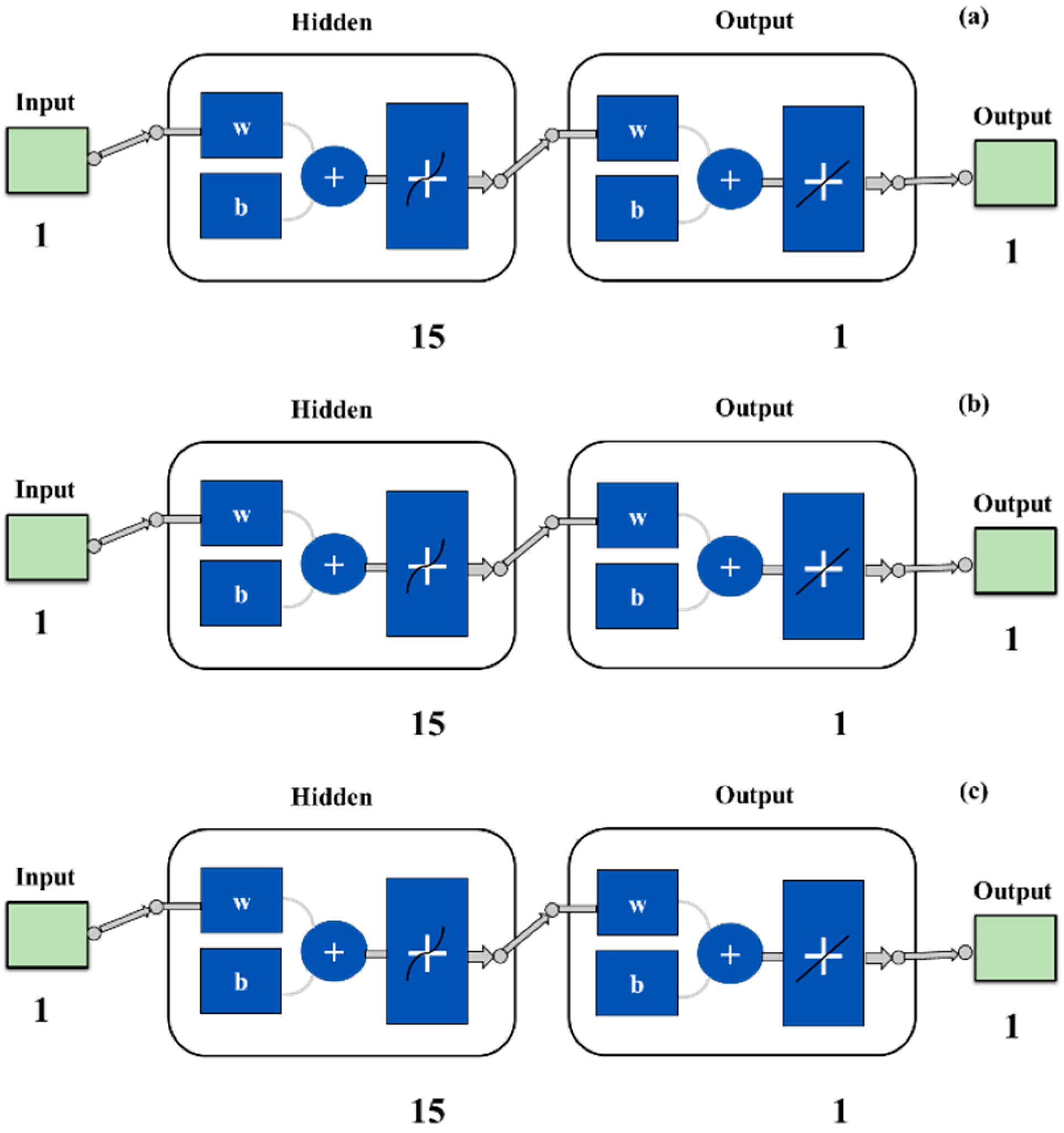
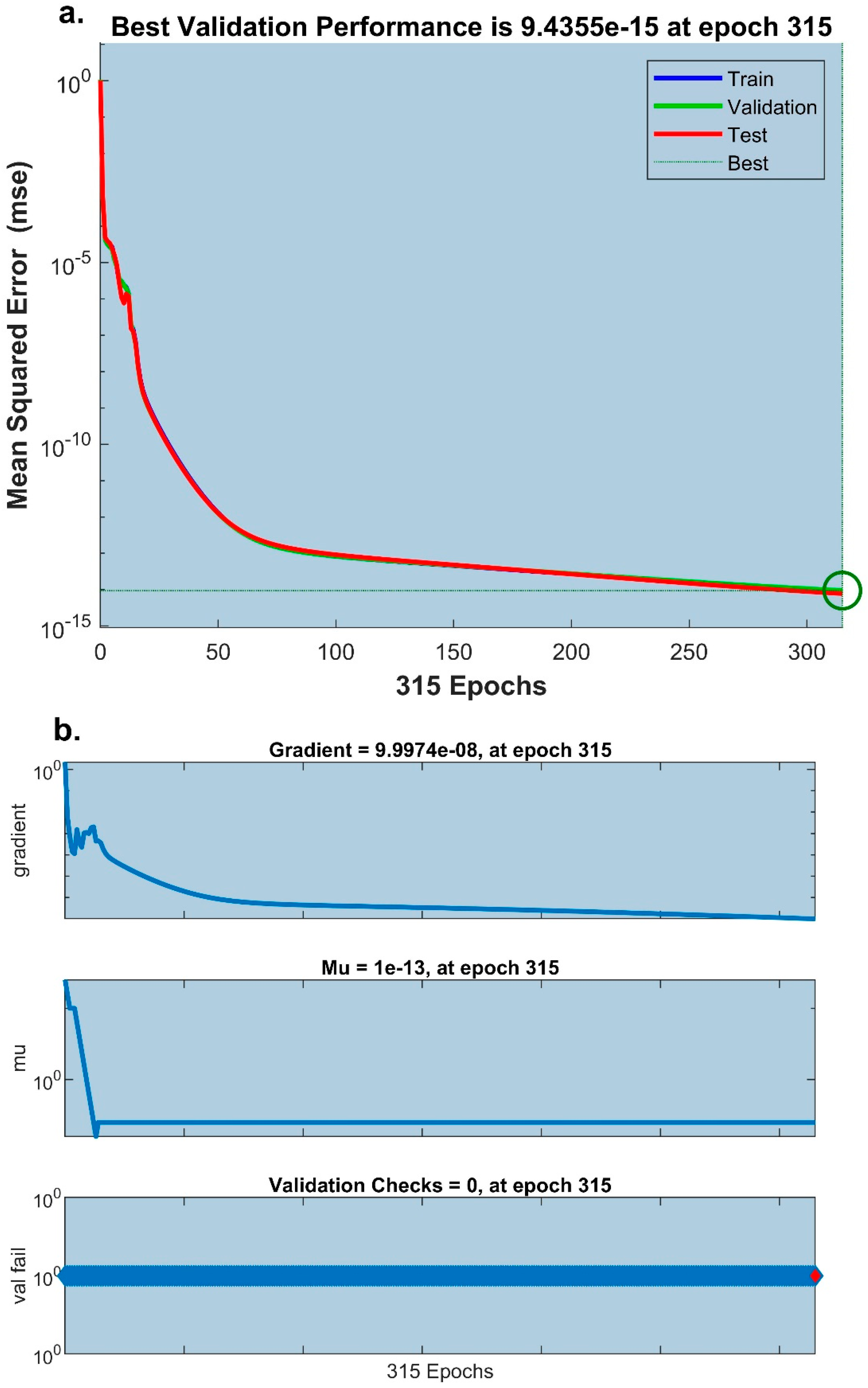
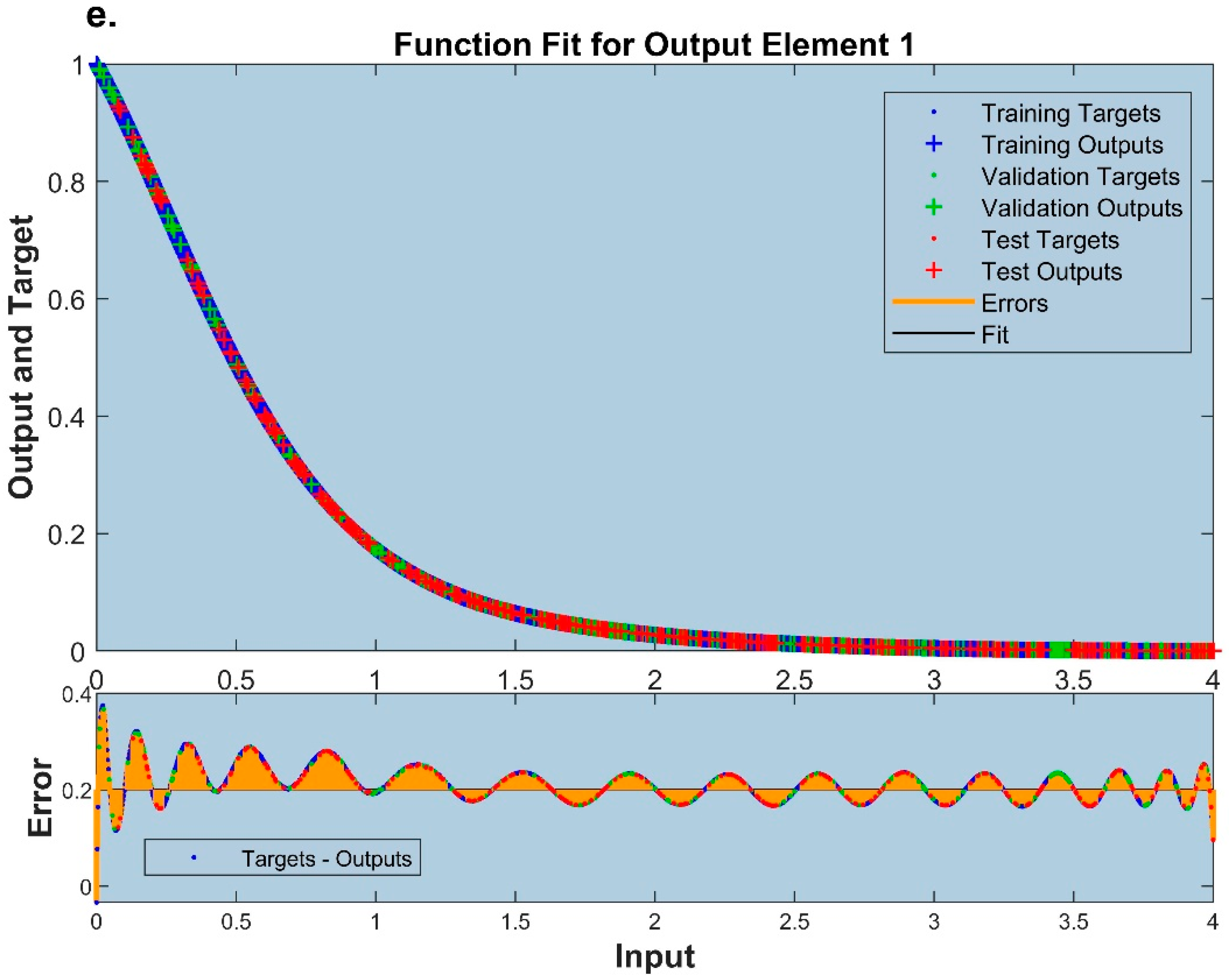
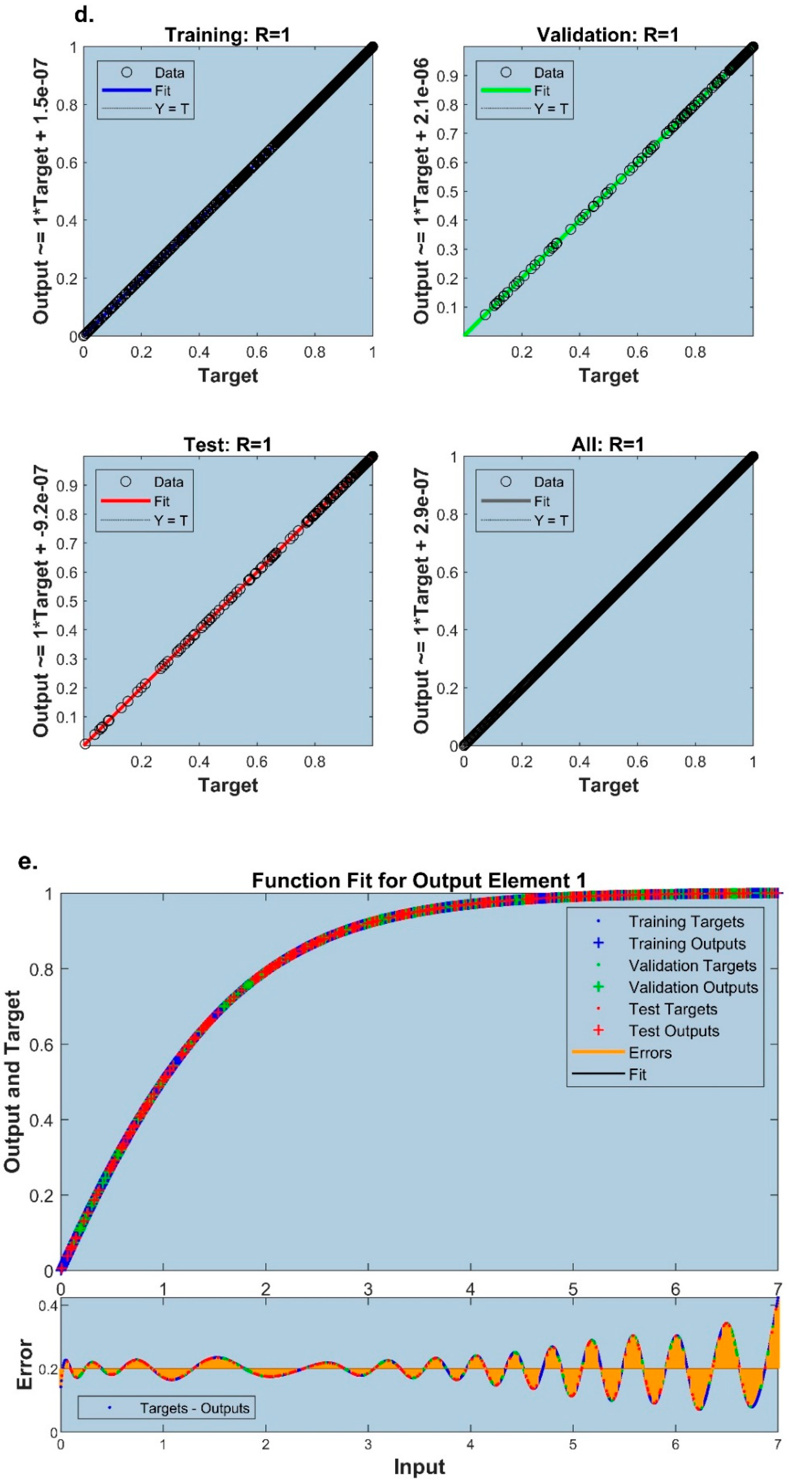
5. Artificial Neural Network Modelling

Artificial Neural Networks (ANNs) offer a highly practical computational model and are frequently used methods for modelling and forecasting the behaviour of highly nonlinear systems. ANNs aim to identify novel patterns by displaying a complicated connection between inputs and outputs. Artificial neural networks are used for various activities, including image identification, medical diagnosis, machine translation and speech recognition. ANNs, modelled after biological nervous systems, consist of a network of interconnected artificial neurons, making them well-suited to replicating the functionality of powerful computer resources.

The present work aimed to provide the models for velocity, thermal and concentration profiles with varying $\eta$ by employing an artificial neural network with the Levenberg–Marquardt scheme (ANN-LMS). The quantity of input and output parameters, the number of layers and connections between neurons, and their design all affect how effectively they work. One input, fifteen hidden neurons and one output are present in the projected velocity, temperature and concentration models. Figure 10 displays the trained ANN-LMS models’ input, hidden, and output layers. In particular, the features of neural network training, including input, hidden, output layers and the number of neurons for the developed ANN-LMS models of velocity, thermal and concentration profiles are presented in the form of model diagrams, as seen in Figure 10a, Figure 10b and Figure 10c, respectively. The weights $\left(w\right)$ and biases $\left(b\right)$ required for predicting the neural network results are also indicated in these figures. The numerical value 1 in the input and output layers mentioned in the figures signify that one set of input and output data is given in both input and output layers for the ANN-LMS model training with 15 hidden neurons in the hidden layer.The dimensionless quantity $\eta$ is transmitted as input to the ANN-LMS’s input layer, and the corresponding data of velocity, thermal and concentration profile procured by solving the dimensionless equations using RKF-45 are provided to the ANN-LMS’s output layer as target sets. The response data of velocity, thermal and concentration profiles are randomly divided, in which 1401, 1501 and 1601 data elements are considered for the training of the corresponding velocity, thermal and concentration profiles models, respectively. For the provided data samples, 70% of the data are used by the proposed ANN-LMS models during the training phase, followed by 15% during the testing and validation phases. Several statistical analyses can measure a model’s effectiveness using the designed ANN-LMS predictions. To systematically establish the performance of ANN-LMS models, performance metrics including mean square error (MSE) and regression coefficient, have been considered to evaluate their performance. The mathematical notations for ANN-LMS performance metrics are as follows:

$$MSE=\frac{1}{n}{\displaystyle \sum _{i=1}^n{({\xi }_{Num(i)}-{\xi }_{ANN(i)})}^2}$$

$$R^2=1-\frac{{\displaystyle \sum _{i=1}^n{({\xi }_{Num(i)}-{\xi }_{ANN(i)})}^2}}{{\displaystyle \sum _{i=1}^n{({\xi }_{Num(i)})}^2}}$$

where $i$ represents the number of data sets, ${\xi }_{Num}$ is the response values of the fluid profiles achieved by employing the numerical technique and ${\xi }_{ANN}$ is the predicted values of the ANN-LMS models.

The validation performance of ANN-LMS models for velocity, thermal and concentration profile is developed in Figure 11a, Figure 12a and Figure 13a, respectively. The best validation performance of $3.0249\times {10}^{-10}$ is reached at epoch 657, together with the lowest MSE for the velocity profile, as shown in Figure 11a. Upon observing Figure 12a, the trained temperature profile model exhibits the lowest MSE magnitude of $9.4355\times {10}^{-15}$ at epoch 315. Further, Figure 13a illustrates the best validation performance for the proposed model of concentration profile with the lowest MSE value of $1.5013\times {10}^{-10}$ attained at epoch 573.

Figure 11b, Figure 12b and Figure 13b represent the Gradient, Mu and validation check of the ANN-LMS concerning the velocity, thermal and concentration profile models, respectively. The Gradient is simply a vector that points the network in the right direction with a certain magnitude to reach the desired results as rapidly as possible, whereas Mu is a factor that controls a specific approach. Mu’s value directly represents the convergence of the solution. Upon observing Figure 11b, for the velocity profile, the gradient value $9.9475\times {10}^{-8}$ is attained at epoch 657 and the corresponding Mu value of $1\times {10}^{-8}$ is achieved. Figure 12b and Figure 13b denote the gradient value $9.9974\times {10}^{-8}$ with Mu value $1\times {10}^{-13}$ at epoch 315 and gradient value $9.9117\times {10}^{-8}$ with Mu value $1\times {10}^{-8}$ at epoch 573 for the temperature profile and concentration profile, respectively.

The error histograms of the constructed ANN-LMS models for velocity, thermal and concentration profiles are shown in Figure 11c, Figure 12c and Figure 13c, respectively. The error histogram shows the distribution of errors away from the zero line. Each bar in the graph represents the number of dataset values that fall into a certain bin. The method’s correctness and stability are confirmed by the fact that the maximum number of values is near the zero-line error. The zero error is attained near the values $2.68\times {10}^{-6}$, $2.14\times {10}^{-9}$ and $8.5\times {10}^{-7}$ for $f^{\prime }(\eta )$, $\theta (\eta )$ and $\chi (\eta )$, respectively.

The regression plot for the training data of the velocity, temperature and concentration profiles is shown in Figure 11d, Figure 12d and Figure 13d, respectively. Regression is a statistical tool used to assess the precision of a trained model by comparing the predicted data points to the regression line. The suggested model’s prediction closely matches the actual values, as indicated by the R value being extremely near to 1. A regression result of 1 indicates a strong correlation between the desired and projected values. Thus, the trained value is achieved at the minimum error for $f^{\prime }(\eta )$, $\theta (\eta )$ and $\chi (\eta )$.

Figure 11e, Figure 12e and Figure 13e explain the fit curve of the ANN-LMS for velocity, temperature and concentration profiles, respectively. These figures show the fitness data based on the difference between the target and network outputs or the difference between the predicted value and target value. The error is discovered to be extremely near to zero, demonstrating the method’s accuracy and suitability. Further,

Table 2. Results of ANN-LMS for velocity profile model.

Epochs	Gradient	Performance	Mu	MSE
				Training	Validation	Testing
$809$	$9.97\times {10}^{-8}$	$3.6\times {10}^{-10}$	$1\times {10}^{-8}$	$3.6011\times {10}^{-10}$	$4.0781\times {10}^{-10}$	$3.9382\times {10}^{-10}$
$677$	$9.96\times {10}^{-8}$	$3.55\times {10}^{-10}$	$1\times {10}^{-8}$	$3.5534\times {10}^{-10}$	$4.3147\times {10}^{-10}$	$3.9013\times {10}^{-10}$
$615$	$1\times {10}^{-7}$	$5.22\times {10}^{-11}$	$1\times {10}^{-8}$	$5.2201\times {10}^{-11}$	$4.7320\times {10}^{-11}$	$5.4119\times {10}^{-11}$

,

Table 3. Results of ANN-LMS for temperature profile model.

Epochs	Gradient	Performance	Mu	MSE
				Training	Validation	Testing
$435$	$9.9\times {10}^{-8}$	$6.17\times {10}^{-14}$	$1\times {10}^{-12}$	$6.1673\times {10}^{-14}$	$6.7780\times {10}^{-14}$	$6.6373\times {10}^{-14}$
$231$	$1\times {10}^{-7}$	$9.83\times {10}^{-15}$	$1\times {10}^{-13}$	$9.8335\times {10}^{-15}$	$1.1768\times {10}^{-14}$	$1.0424\times {10}^{-14}$
$179$	$9.9\times {10}^{-8}$	$1.91\times {10}^{-14}$	$1\times {10}^{-13}$	$1.9103\times {10}^{-14}$	$1.9818\times {10}^{-14}$	$2.1127\times {10}^{-14}$

and

Table 4. Results of ANN-LMS for concentration profile model.

Epochs	Gradient	Performance	Mu	MSE
				Training	Validation	Testing
$660$	$9.98\times {10}^{-8}$	$1.63\times {10}^{-10}$	$1\times {10}^{-8}$	$1.6293\times {10}^{-10}$	$1.3177\times {10}^{-10}$	$1.6802\times {10}^{-10}$
$589$	$9.94\times {10}^{-8}$	$1.4\times {10}^{-10}$	$1\times {10}^{-8}$	$1.3993\times {10}^{-10}$	$1.6688\times {10}^{-10}$	$1.4285\times {10}^{-10}$
$575$	$9.99\times {10}^{-8}$	$1.76\times {10}^{-10}$	$1\times {10}^{-8}$	$1.7559\times {10}^{-10}$	$1.4423\times {10}^{-10}$	$2.0142\times {10}^{-10}$

denote the achieved results of ANN-LMS models for the velocity, temperature and concentration profiles at different epochs.

6. Conclusions

The current study explores the time-dependent Maxwell nanofluid flow with thermophoretic particle deposition by considering the solid–liquid interfacial layer and nanoparticle diameter. The non-linear governing equations are converted into ordinary differential equations using suitable similarity variables. These reduced equations are solved using the Runge–Kutta Fehlberg-45 method with the shooting technique. Visual aids such as graphs and tables effectively convey the quantitative results. The results reveal that the velocity profile drops with an upsurge in unsteadiness parameter and Deborah number values. The increase in the values of space and temperature-dependent heat source/sink parameters increases the temperature. The concentration profile declines as the thermophoretic parameter upsurges. Finally, the method’s correctness and stability are confirmed because the maximum number of values is near the zero-line error. The zero error is attained near the values $2.68\times {10}^{-6}$, $2.14\times {10}^{-9}$ and $8.5\times {10}^{-7}$ for velocity, thermal and concentration profiles, respectively.

References

1. Shahid, A. The Effectiveness of Mass Transfer in the MHD Upper-Convected Maxwell Fluid Flow on a Stretched Porous Sheet near Stagnation Point: A Numerical Investigation. Inventions 2020, 5, 64. [Google Scholar] [CrossRef]
2. Megahed, A.M. Improvement of heat transfer mechanism through a Maxwell fluid flow over a stretching sheet embedded in a porous medium and convectively heated. Math. Comput. Simul. 2021, 187, 97–109. [Google Scholar] [CrossRef]
3. Gowda, R.J.P.; Rauf, A.; Kumar, R.N.; Prasannakumara, B.C.; Shehzad, S.A. Slip flow of Casson–Maxwell nanofluid confined through stretchable disks. Indian J. Phys. 2022, 96, 2041–2049. [Google Scholar] [CrossRef]
4. Bhatti, M.M.; Shahid, A.; Sarris, I.E.; Bég, O.A. Spectral relaxation computation of Maxwell fluid flow from a stretching surface with quadratic convection and non-Fourier heat flux using Lie symmetry transformations. Int. J. Mod. Phys. B 2023, 37, 2350082. [Google Scholar] [CrossRef]
5. Abbas, A.; Wakif, A.; Shafique, M.; Ahmad, H.; ul Ain, Q.; Muhammad, T. Thermal and mass aspects of Maxwell fluid flows over a moving inclined surface via generalized Fourier’s and Fick’s laws. Waves Random Complex Media 2023, 1–27. [Google Scholar] [CrossRef]
6. Khan, N.M.; Chu, Y.-M.; Khan, M.I.; Kadry, S.; Qayyum, S. Modeling and dual solutions for magnetized mixed convective stagnation point flow of upper convected Maxwell fluid model with second-order velocity slip. Math. Methods Appl. Sci. 2020. [Google Scholar] [CrossRef]
7. Fetecau, C.; Rauf, A.; Qureshi, T.M.; Mehmood, O.U. Analytical solutions of upper-convected Maxwell fluid flow with exponential dependence of viscosity on the pressure. Eur. J. Mech. B/Fluids 2021, 88, 148–159. [Google Scholar] [CrossRef]
8. Fayz-Al-Asad, M.; Oreyeni, T.; Yavuz, M.; Olanrewaju, P.O. Analytic simulation of MHD boundary layer flow of a chemically reacting upper-convected Maxwell fluid past a vertical surface subjected to double stratifications with variable properties. Eur. Phys. J. Plus 2022, 137, 813. [Google Scholar] [CrossRef]
9. Waqas, H.; Farooq, U.; Hussain, M.; Alanazi, A.K.; Brahmia, A.; Hammouch, Z.; Abo-Dief, H.M.; Safaei, M.R. Cattaneo-Christov heat and mass flux effect on upper-convected Maxwell nanofluid with gyrotactic motile microorganisms over a porous sheet. Sustain. Energy Technol. Assess. 2022, 52, 102037. [Google Scholar] [CrossRef]
10. Muhammad, M.H.; Abas, S.S.; Jaafar, N.A.; Usman, A.; Mamat, M. Mathematical Modeling on Magnetohydrodynamics Upper Convected Maxwell Fluid Flow Past a Flat Plate Using Spectral Relaxation Approach. J. Adv. Res. Fluid Mech. Therm. Sci. 2023, 106, 23–38. [Google Scholar] [CrossRef]
11. Gowda, R.P.; Kumar, R.N.; Aldalbahi, A.; Issakhov, A.; Prasannakumara, B.C.; Rahimi-Gorji, M.; Rahaman, M. Thermophoretic particle deposition in time-dependent flow of hybrid nanofluid over rotating and vertically upward/ downward moving disk. Surf. Interfaces 2021, 22, 100864. [Google Scholar] [CrossRef]
12. Shehzad, S.A.; Mabood, F.; Rauf, A.; Tlili, I. Forced convective Maxwell fluid flow through rotating disk under the thermophoretic particles motion. Int. Commun. Heat Mass Transf. 2020, 116, 104693. [Google Scholar] [CrossRef]
13. Kumar, R.N.; Jyothi, A.M.; Alhumade, H.; Gowda, R.P.; Alam, M.M.; Ahmad, I.; Gorji, M.R.; Prasannakumara, B.C. Impact of magnetic dipole on thermophoretic particle deposition in the flow of Maxwell fluid over a stretching sheet. J. Mol. Liq. 2021, 334, 116494. [Google Scholar] [CrossRef]
14. Bashir, S.; Ramzan, M.; Ghazwani, H.A.S.; Nisar, K.S.; Saleel, C.A.; Abdelrahman, A. Magnetic Dipole and Thermophoretic Particle Deposition Impact on Bioconvective Oldroyd-B Fluid Flow over a Stretching Surface with Cattaneo–Christov Heat Flux. Nanomaterials 2022, 12, 2181. [Google Scholar] [CrossRef] [PubMed]
15. Kumar, R.N.; Gowda, R.J.P.; Madhukesh, J.K.; Prasannakumara, B.C.; Ramesh, G.K. Impact of thermophoretic particle deposition on heat and mass transfer across the dynamics of Casson fluid flow over a moving thin needle. Phys. Scr. 2021, 96, 075210. [Google Scholar] [CrossRef]
16. Ahmad, F.; Abdal, S.; Ayed, H.; Hussain, S.; Salim, S.; Almatroud, A.O. The improved thermal efficiency of Maxwell hybrid nanofluid comprising of graphene oxide plus silver / kerosene oil over stretching sheet. Case Stud. Therm. Eng. 2021, 27, 101257. [Google Scholar] [CrossRef]
17. Chandrasekaran, S.; Gupta, M.S.; Jangid, S.; Loganathan, K.; Deepa, B.; Chaudhary, D.K. Unsteady Radiative Maxwell Fluid Flow over an Expanding Sheet with Sodium Alginate Water-Based Copper-Graphene Oxide Hybrid Nanomaterial: An Application to Solar Aircraft. Adv. Mater. Sci. Eng. 2022, 2022, e8622510. [Google Scholar] [CrossRef]
18. Bhattacharyya, A.; Sharma, R.; Hussain, S.M.; Chamkha, A.J.; Mamatha, E. A numerical and statistical approach to capture the flow characteristics of Maxwell hybrid nanofluid containing copper and graphene nanoparticles. Chin. J. Phys. 2022, 77, 1278–1290. [Google Scholar] [CrossRef]
19. Hussain, S.M.; Sharma, R.; Mishra, M.R.; Alrashidy, S.S. Hydromagnetic Dissipative and Radiative Graphene Maxwell Nanofluid Flow Past a Stretched Sheet-Numerical and Statistical Analysis. Mathematics 2020, 8, 1929. [Google Scholar] [CrossRef]
20. Algehyne, E.A.; Rehman, S.; Ayub, R.; Saeed, A.; Eldin, S.M.; Galal, A.M. Brownian and thermal diffusivity impact due to the Maxwell nanofluid (graphene/engine oil) flow with motile microorganisms and Joule heating. Nanotechnol. Rev. 2023, 12, 20220540. [Google Scholar] [CrossRef]
21. Jamshed, W.; Safdar, R.; Rehman, Z.; Lashin, M.M.; Ehab, M.; Moussa, M.; Rehman, A. Computational technique of thermal comparative examination of Cu and Au nanoparticles suspended in sodium alginate as Sutterby nanofluid via extending PTSC surface. J. Appl. Biomater. Funct. Mater. 2022, 20, 22808000221104004. [Google Scholar] [CrossRef]
22. Tassaddiq, A.; Khan, I.; Nisar, K.S. Heat transfer analysis in sodium alginate based nanofluid using MoS2 nanoparticles: Atangana–Baleanu fractional model. Chaos Solitons Fractals 2020, 130, 109445. [Google Scholar] [CrossRef]
23. Shaukat, A.; Mushtaq, M.; Farid, S.; Jabeen, K.; Muntazir, R.M.A. A Study of Magnetic/Nonmagnetic Nanoparticles Fluid Flow under the Influence of Nonlinear Thermal Radiation. Math. Probl. Eng. 2021, 2021, 210414. [Google Scholar] [CrossRef]
24. Raza, A.; Almusawa, M.Y.; Ali, Q.; Haq, A.U.; Al-Khaled, K.; Sarris, I.E. Solution of Water and Sodium Alginate-Based Casson Type Hybrid Nanofluid with Slip and Sinusoidal Heat Conditions: A Prabhakar Fractional Derivative Approach. Symmetry 2022, 14, 2658. [Google Scholar] [CrossRef]
25. Dawar, A.; Islam, S.; Shah, Z.; Mahmuod, S.R. A passive control of Casson hybrid nanofluid flow over a curved surface with alumina and copper nanomaterials: A study on sodium alginate-based fluid. J. Mol. Liq. 2023, 382, 122018. [Google Scholar] [CrossRef]
26. Alizadeh-Pahlavan, A.; Sadeghy, K. On the use of homotopy analysis method for solving unsteady MHD flow of Maxwellian fluids above impulsively stretching sheets. Commun. Nonlinear Sci. Numer. Simulat. 2009, 14, 1355–1365. [Google Scholar] [CrossRef]
27. Shateyi, S.; Muzara, H. A numerical analysis on the unsteady flow of a thermomagnetic reactive Maxwell nanofluid over a stretching/shrinking sheet with ohmic dissipation and Brownian motion. Fluids 2022, 7, 252. [Google Scholar] [CrossRef]
28. Shankaralingappa, B.M.; Madhukesh, J.K.; Sarris, I.E.; Gireesha, B.J.; Prasannakumara, B.C. Influence of thermophoretic particle deposition on the 3D flow of sodium alginate-based Casson nanofluid over a stretching sheet. Micromachines 2021, 12, 1474. [Google Scholar] [CrossRef] [PubMed]
29. Hayat, T.; Asad, S.; Mustafa, M.; Alsaedi, A. Radiation effects on the flow of Powell-Eyring fluid past an unsteady inclined stretching sheet with non-uniform heat source/sink. PLoS ONE 2014, 9, e103214. [Google Scholar]
30. Acharya, N.; Mabood, F.; Shahzad, S.A.; Badruddin, I.A. Hydrothermal variations of radiative nanofluid flow by the influence of nanoparticles diameter and nanolayer. Int. Commun. Heat Mass Transf. 2022, 130, 105781. [Google Scholar] [CrossRef]
31. Obalalu, A.M.; Salawu, S.O.; Memon, M.A.; Olayemi, O.A.; Ali, M.R.; Sadat, R.; Odetunde, C.B.; Ajala, O.A.; Akindele, A.O. Akindele. Computational study of Cattaneo–Christov heat flux on cylindrical surfaces using CNT hybrid nanofluids: A solar-powered ship implementation. Case Stud. Therm. Eng. 2023, 45, 102959. [Google Scholar] [CrossRef]
32. Obalalu, A.M.; Memon, M.A.; Olayemi, O.A.; Olilima, J.; Fenta, A. Enhancing heat transfer in solar-powered ships: A study on hybrid nanofluids with carbon nanotubes and their application in parabolic trough solar collectors with electromagnetic controls. Sci. Rep. 2023, 13, 9476. [Google Scholar] [CrossRef]
33. Obalalu, A.M.; Olayemi, O.A.; Olakunle, S.S.; Bode Odetunde, C. Scrutinization of Solar Thermal Energy and Variable Thermophysical Properties Effects on Non-Newtonian Nanofluid Flow. Int. J. Eng. Res. Afr. 2023, 64, 93–115. [Google Scholar] [CrossRef]
34. Hamilton, R.L.; Crosser, O.K. Thermal conductivity of heterogeneous two-component systems. Ind. Eng. Chem. Fundam. 1962, 1, 187–191. [Google Scholar] [CrossRef]
35. Murshed, S.M.S.; Leong, K.C.; Yang, C. Investigations of thermal conductivity and viscosity of nanofluids. Int. J. Therm. Sci. 2008, 47, 560–568. [Google Scholar] [CrossRef]
36. Leong, K.C.; Yang, C.; Murshed, S.M.S. A model for the thermal conductivity of nanofluids—The effect of interfacial layer. J. Nanopart. Res. 2006, 8, 245–254. [Google Scholar] [CrossRef]
37. Xue, L.; Keblinski, P.; Phillpot, S.R.; Choi, S.S.; Eastman, J.A. Effect of liquid layering at the liquid–solid interface on thermal transport. Int. J. Heat Mass Transf. 2004, 47, 4277–4284. [Google Scholar] [CrossRef]
38. Yu, C.J.; Richter, A.G.; Datta, A.; Durbin, M.K.; Dutta, P. Molecular layering in a liquid on a solid substrate: An X-ray reflectivity study. Phys. B Condens. Matter 2000, 283, 27–31. [Google Scholar] [CrossRef]
39. Talbot, L.; Cheng, R.K.; Schefer, A.W.; Wills, D.R. Thermophoresis of particles in a 552 heated boundary layer. J. Fluid Mech. 1980, 101, 737–758. [Google Scholar] [CrossRef] [Green Version]
Figure 1. Effect of Deborah number on velocity profile.
Mathematics 11 03501 g001
Figure 2. Effect of Deborah number on thermal profile.
Mathematics 11 03501 g002
Figure 3. Effect of unsteadiness parameter on velocity profile.
Mathematics 11 03501 g003
Figure 4. Effect of unsteadiness parameter on thermal profile.
Mathematics 11 03501 g004
Figure 5. Effect of space-dependent internal heat generation/absorption parameter on thermal profile.
Mathematics 11 03501 g005
Figure 6. Effect of temperature-dependent internal heat generation/absorption parameter on thermal profile.
Mathematics 11 03501 g006
Figure 7. Effect of Schmidt number on concentration profile.
Mathematics 11 03501 g007
Figure 8. Effect of thermophoretic parameter on concentration profile.
Mathematics 11 03501 g008
Figure 9. Effect of nanoparticle diameter on thermal profile.
Mathematics 11 03501 g009
Figure 10. ANN design for (a) velocity profile model (b) temperature profile model (c) concentration profile model.
Mathematics 11 03501 g010
Figure 11. (a) Performance of ANN-LMS, (b) training plot, (c) error distribution plot, (d) regression plot, (e) fitness plot for velocity profiles.
Mathematics 11 03501 g011aMathematics 11 03501 g011bMathematics 11 03501 g011c
Figure 12. (a) Performance of ANN-LMS, (b) training plot, (c) error distribution plot, (d) regression plot, (e) fitness plot for temperature profiles.
Mathematics 11 03501 g012aMathematics 11 03501 g012bMathematics 11 03501 g012c
Figure 13. (a) Performance of ANN-LMS, (b) training plot, (c) error distribution plot, (d) regression plot, (e) fitness plot for concentration profiles.
Mathematics 11 03501 g013aMathematics 11 03501 g013bMathematics 11 03501 g013c