Forecasting Day-Ahead Brent Crude Oil Prices Using Hybrid Combinations of Time Series Models

Abstract

Crude oil price forecasting is an important research area in the international bulk commodity market. However, as risk factors diversify, price movements exhibit more complex nonlinear behavior. Hence, this study provides a comprehensive analysis of forecasting Brent crude oil prices by comparing various hybrid combinations of linear and nonlinear time series models. To this end, first, the logarithmic transformation is used to stabilize the variance of the crude oil prices time series; second, the original time series of log crude oil prices is decomposed into two new subseries, such as a long-run trend series and a stochastic series, using the Hodrick–Prescott filter; and third, two linear and two nonlinear time series models are considered to forecast the decomposed subseries. Finally, the forecast results for each subseries are combined to obtain the final day-ahead forecast result. The proposed modeling framework is applied to daily Brent spot prices from 1 January 2013 to 27 December 2022. Six different accuracy metrics, pictorial analysis, and a statistical test are performed to verify the proposed methodology’s performance. The experimental results (accuracy measures, pictorial analysis, and statistical test) show the efficiency and accuracy of the proposed hybrid forecasting methodology. Additionally, our forecasting results are comparatively better than the benchmark models. Finally, we believe that the proposed forecasting method can be used for other complex financial time data to obtain highly efficient and accurate forecasts.

1. Introduction

The price of commodities in the international market varies significantly and rises over time. The fluctuation in commodity prices has a significant impact on the world economy, increasing import costs, promoting inflation, stifling economic growth, and reducing the effectiveness of macroeconomic policy [1]. Therefore, the global economy must analyze the features of variations in commodities sold on foreign markets to forecast their price and their historical patterns.

As one of the most important energy resources and one of the most widely traded commodities, crude oil is crucial to the global economic system. It is well known for having significant price changes that directly affect the world economy. Crude oil, an essential component of industrial production, has a significant impact on the growth and stabilization of the world economy and the international financial markets. Crude oil price changes have a severe impact on the development and safety of nations worldwide by limiting their growth and destabilizing the global economy [2]. Oil importers may experience inflation and other economic effects as oil prices rise, whereas oil exporters may experience an economic slump and political unrest as oil prices decrease [3].

Due to the above-stated factors, researchers have paid a lot of attention to the energy crisis and the volatile petroleum price [4,5]. Crude oil is a commodity with significant worldwide influence because it is the key source of primary energy. However, predicting the price of oil is a difficult task since many factors (global economic conditions, speculative expectations, extreme events, political instabilities, and technological trends) influence oil pricing, and the strengths of these factors change over time [6,7]. Because of the above-mentioned factors, forecasting day-ahead crude oil prices is one of the most important and challenging tasks and attracts the attention of researchers.

According to the literature, the price of crude oil has been predicted using different types of forecasting techniques. These predictive models can be broadly classified into three main categories: (a) statistical and econometric models; (b) machine learning algorithms; and (c) hybrid models. Statistical and econometric models used for crude oil forecasting include random walk, autoregressive, autoregressive integrated moving average, autoregressive conditional heteroscedasticity, generalized autoregressive conditional heteroscedasticity, vector autoregressive, vector error correction models, etc. [8,9]. For instance, Xiong and Wu [10] employed the vector error correction (VEC) model and cointegration analysis to forecast the demand for crude oil in China. Gülen [11] also forecasts the West Texas Intermediate (WTI) crude oil price by using the cointegration methodology. Lanza et al. [12] used the error correction model (ECM) specification to predict crude oil prices. Drachal [13] used the vector autoregression model (VAR) and found that these models are more accurate than single equation models for forecasting. Ahmad [14] used Box–Jenkins approaches to examine Oman’s average monthly crude oil prices and recommended the seasonal model ARIMA $(1,1,5)(1,1,1)$. Morana [15] forecasted the oil prices for short-term horizons by using the semiparametric generalized autoregressive conditional heteroscedasticity (GARCH) model. Mohammadi and Su [16] evaluated the predictions of several ARIMA-GARCH models on the weekly prices of crude oil in eleven global markets. Hou and Suardi [17] used a nonparametric GARCH model, which indicates that this approach provides an appealing and practical substitute for the widely used parametric GARCH models. Joshi [18] used a linear regression model to forecast oil prices. One of the main assumptions of econometric and statistical models is linearity, and they provide good results when the price series are linear or close to linear. These models might not be the best choice, because there is a lot of nonlinearity and inconsistency in the observed crude oil price series [19].

On the other hand, the price forecasting literature has developed and used several machine learning models, including support vector machines, genetic algorithms, and artificial neural networks, in response to the shortcomings of statistical and econometric methodologies. For example, a neural network model was developed by Movagharnejad et al. [20] to analyze the price changes in different commercial oils in the Persian Gulf region. Mirmirani and Li [21] used vector autoregression and artificial neural networks to investigate US oil prices and suggested that in forecasting, a BPN-GA model can perform better than a VAR model. Through the use of the hierarchical conceptual (HC) and artificial neural networks-quantitative (NNA-Q) models, machine learning and computational intelligence techniques are used to forecast the monthly WTI crude oil price for each barrel in US dollars. The outcome of the simulation analysis verified the efficiency of the HC model’s data selection method [22]. Xie et al. [23] suggested a new SVM-based technique to forecast the price of crude oil. They compared SVM’s performance with that of ARIMA and BPNN to assess its potential for forecasting. Several studies have shown that when it comes to price prediction, AI models frequently outperform traditional time series models [19,24,25]. Moreover, AI models can have flaws and limitations of their own. For instance, the choice of parameters affects NNAs [19]. Other proposals fir time series analysis and forecasting can be found in [26,27,28,29] and references therein.

The complexity of oil pricing is due to relevant time series frequently including lag, nonlinearity, and connections to several markets. It has been difficult in the literature to suggest a hybrid model that can both capture and optimize these aspects. Abdollahi, H., and Ebrahimi, S. B. [30] proposed a hybrid model to forecast daily Brent crude oil prices with the lowest possible forecasting error and, more importantly, to introduce a hybridization that is best able to capture the key characteristics of the oil price time series, including nonlinearity, lag, and market interactions.

In recent studies, Chen, Z. et al. [31] used the MIDAS modeling framework, which is a common mixed data sampling approach, to investigate how leverage and jumps affect the ability to forecast the realized volatility (RV) of China’s crude oil futures. This study’s findings can be utilized to better predict the volatility of China’s crude oil futures, reduce investment risks, and provide higher profits. Salisu, A. A., et al. [32] found that the GARCH-MIDAS-X model for oil volatility forecast accuracy is improved by considering any inherent asymmetries in the global economic activity proxies. The findings that led to these conclusions are valid across a range of forecast periods and alternative energy sources. The Musetescu, R.C., et al. [33] approach involves forecasting conditional variance over two distinct periods, 20 May 1987 to 24 January 2022 and 20 January 2020 to 24 January 2022. In comparison to the model GARCH-M (1,1), which is appropriate for the period 2020–2022, the forecasting results showed that GARCH (1,1) was the model with the highest level of crude oil volatility anticipated for the entire time. Xing, L. M. and Zhang, Y. J. [34] studied various shrinkage mechanism specifications to forecast the crude oil price and evaluated the prediction effectiveness from both a statistical and an economic standpoint. By considering the nonlinear forms of predictors, Zhang, Y., et al.’s [35] study aimed to enhance the forecasting capabilities of diffusion index (DI) models. To be more precise, they used principal component analysis (PCA) and partial least squares (PLS), two popular DI models, to forecast monthly crude oil returns.

In today’s modern world, day-ahead forecasting is beneficial for operational planning, enabling companies to efficiently change production schedules, improve logistics, and allocate resources. On the other hand, short-term forecasting facilitates risk management by allowing traders to measure market volatility and control portfolio risk. In addition, accurate and efficient day-ahead forecasts help energy traders to make wise judgments concerning purchases and sales of energy commodities. Therefore, this study provides a comprehensive analysis of forecasting Brent crude oil prices by comparing various hybrid combinations of linear and nonlinear time series models. To this end, first, the logarithmic transformation is used to stabilize the variance of the crude oil prices time series; second, the original time series of log crude oil prices is decomposed into two new subseries, a long-run trend series, and a stochastic series, using the Hodrick–Prescott filter; and third, two linear and two nonlinear time series models are considered to forecast the decomposed subseries. Finally, the forecast results for each subseries are combined to obtain the final day-ahead forecast. The proposed modeling framework is applied to daily Brent spot prices from 1 January 2013 to 27 December 2022.

The remainder of the paper is designed as follows: Section 2 comprises the general procedure of the proposed hybrid forecasting approach. Section 3 contains an empirical application of the proposed forecasting methodology using the daily Brent oil price data. Section 4 details the discussion of the proposed best combination model versus the considered standard linear and nonlinear time series benchmark models. Finally, Section 5 covers the conclusions, limitations, and future research directions.

2. The Proposed Hybrid Forecasting Methodology

This section explains the proposed hybrid forecasting methodology for daily Brent oil spot prices forecasting. The Brent spot price time series exhibits nonlinear and complex characteristics. To achieve this, the original time series of Brent spot prices (${\mathrm{B}}_{\mathrm{t}}$) is decomposed into two subseries, the long-term nonlinear trend (${\mathrm{n}}_{\mathrm{t}}$) and a stochastic (residual) (${\mathrm{s}}_{\mathrm{t}}$) series, using the Hodrick–Prescott filter. The mathematical representation of the decomposed components is given by

$${\mathrm{B}}_{\mathrm{t}}={\mathrm{n}}_{\mathrm{t}}+{\mathrm{s}}_{\mathrm{t}}$$

(1)

the Hodrick–Prescott Filter is described in the following subsection.

2.1. Hodrick–Prescott Filter

A smoothed-curve representation of a time series that is more complex to long-term variations than to short-term fluctuations is obtained by using the Hodrick–Prescott filter (HPF). The adjustment of the sensitivity of the trend to short-term fluctuations is achieved by modifying a multiplier $\lambda$. Let ${\mathrm{B}}_{\mathrm{t}}$($\mathrm{t}=1,2,\dots ,\mathrm{T}$) denote the time series data. The series ${\mathrm{B}}_{\mathrm{t}}$ is made up of a trend component denoted by ${\mathrm{n}}_{\mathrm{t}}$, and error component, denoted by $\epsilon$, and can be written as;

$${\mathrm{B}}_{\mathrm{t}}={\mathrm{n}}_{\mathrm{t}}+{\epsilon }_{\mathrm{t}}$$

(2)

here, we insert a long-term trend component that can be estimated by minimizing the following expression:

$${\mathrm{minB}}_{\mathrm{t}}\left({\Sigma }_{\mathrm{t}=1}^{\mathrm{T}}{({\mathrm{B}}_{\mathrm{t}}-{\mathrm{n}}_{\mathrm{t}})}^2+\alpha {\Sigma }_{\mathrm{t}=2}^{\mathrm{T}-1}{\left[({\mathrm{n}}_{\mathrm{t}+1}-{\mathrm{n}}_{\mathrm{t}})-({\mathrm{n}}_{\mathrm{t}}-{\mathrm{n}}_{\mathrm{t}-1})\right]}^2\right)$$

(3)

the first term in the above equation is the loss function, and the second is $\alpha$ multiplied by the sum of the squares of the second differences of the long-term trend series, penalizing changes in the growth rate of the long-term trend series.

Figure 1 illustrates the performance of the HP filter by presenting a graphical representation of the new subseries decomposition. The figure consists of three panels, showcasing the original time series of Brent oil prices, the nonlinear long-run trend denoted as ${\mathrm{B}}_{\mathrm{t}}$, and the stochastic (residual) series. From the figure, it is evident that the HPF decomposition successfully captures the dynamics of the series. The nonlinear long-run trend, represented by ${\mathrm{B}}_{\mathrm{t}}$, effectively captures the fluctuations observed in the daily spot Brent prices time series.

2.2. Modeling to Filtered Series

After extracting the subseries from the original time series of Brent oil prices (${\mathrm{B}}_{\mathrm{t}}$) using the HPF, the next step is to estimate the extracted series using four commonly used time series models. These models include two linear models: autoregressive (AR) and autoregressive moving average (ARMA), as well as two nonlinear models: nonlinear autoregressive (NPAR) and nonlinear autoregressive neural network (NNA). These models are detailed in the next subsections.

2.2.1. Autoregressive Model

A linear and parametric autoregressive (AR) process describes the short-term dynamics of ${\mathrm{B}}_{\mathrm{t}}$ and considers a linear combination of the previous time (lag) q observations of ${\mathrm{B}}_{\mathrm{t}}$. It can be written as:

$${\mathrm{B}}_{\mathrm{t}}=\mu +{\gamma }_1{\mathrm{B}}_{\mathrm{t}-1}+{\gamma }_2{\mathrm{B}}_{\mathrm{t}-2}+\dots +{\gamma }_{\mathrm{q}}{\mathrm{B}}_{\mathrm{t}-\mathrm{q}}+{ϵ}_{\mathrm{t}}$$

(4)

where $\mu$ and ${\gamma }_{\mathrm{i}}(\mathrm{i}=1,2,\dots ,\mathrm{q})$ are the intercept and slope parameters of the underlying AR process, and ${ϵ}_{\mathrm{t}}$ is the disturbance term. Based on the autocorrelation and partial autocorrelation functions, the AR(3) model is the most appropriate to model ${\mathrm{B}}_{\mathrm{t}}$.

2.2.2. Autoregressive Moving Average Model

The autoregressive moving average (ARMA) model is a powerful approach that takes into account not only the past values of the target variable but also incorporates relevant information through moving average terms. In the context of the current study variable, ${\mathrm{B}}_{\mathrm{t}}$, the ARMA model explains its behavior based on the previous r terms as well as the lagged values of residuals. By considering both autoregressive and moving average components, the ARMA model provides a comprehensive framework for capturing the dynamics of the variable of interest. The model can be written as

$${\mathrm{B}}_{\mathrm{t}}=\mu +{\gamma }_1{\mathrm{B}}_{\mathrm{t}-1}+{\gamma }_2{\mathrm{B}}_{\mathrm{t}-2}+\dots +{\gamma }_{\mathrm{q}}{\mathrm{B}}_{\mathrm{t}-\mathrm{q}}+{ϵ}_{\mathrm{t}}+{\varphi }_1{ϵ}_{\mathrm{t}-1}+{\varphi }_2{ϵ}_{\mathrm{t}-2}+\dots +{\varphi }_{\mathrm{r}}{ϵ}_{\mathrm{t}-\mathrm{r}}$$

(5)

where $\mu$ is the intercept, ${\gamma }_{\mathrm{i}}(\mathrm{i}=1,2,\dots ,\mathrm{q})$ and ${\varphi }_{\mathrm{k}}(\mathrm{k}=1,2,\dots ,\mathrm{r})$ are the parameters of the AR and MA processes, respectively, and ${ϵ}_{\mathrm{t}}$ is the white noise, a Gaussian sequence with mean zero and variance ${\sigma }_{ϵ}^2$. Based on the autocorrelation and partial autocorrelation functions, the ARMA(3,1) model is the most appropriate to model ${\mathrm{B}}_{\mathrm{t}}$.

2.2.3. Nonparametric Autoregressive Model

The additive nonparametric counterpart of the autoregressive (AR) process gives rise to the additive model (NPAR). In this model, the relationship between ${\mathrm{B}}_{\mathrm{t}}$ and its previous terms is not constrained by a specific parametric form, allowing for the inclusion of various types of nonlinearities. The NPAR model provides flexibility in capturing nonlinear patterns and dependencies within the data, enabling a more comprehensive and flexible representation of the underlying dynamics, and can be written as

$${\mathrm{B}}_{\mathrm{t}}={\mathrm{g}}_1\left({\mathrm{B}}_{\mathrm{t}-1}\right)+{\mathrm{g}}_2\left({\mathrm{B}}_{\mathrm{t}-2}\right)+\dots +{\mathrm{g}}_{\mathrm{q}}({\mathrm{B}}_{\mathrm{t}-\mathrm{q}})+{ϵ}_{\mathrm{t}}$$

(6)

where ${\mathrm{g}}_{\mathrm{i}}$$(\mathrm{i}=1,2,\dots ,\mathrm{q})$ are smoothing functions and describe the association between ${\mathrm{B}}_{\mathrm{t}}$ and its past values. In this work, the functions ${\mathrm{g}}_{\mathrm{i}}$ are represented by a cubic regression spline. Similarly to its parametric counterpart, we consider three lags to estimate NPAR.

2.2.4. Nonlinear Autoregressive Neural Network

The nonlinear autoregressive neural network (NNA) is a machine learning model specifically designed for forecasting future values of input variables. The NNA model utilizes a re-injection mechanism to predict future values of a time series based on its past values. This mechanism allows for the incorporation of expected values, which are then used as inputs for new forecasts at subsequent time points. During the network’s training phase, an open-loop approach is employed, where actual target values are used as feedback to ensure higher accuracy. Once the training process is completed, the network is transformed into a closed loop, and the forecasted values are used as new feedback inputs, enabling the model to make accurate predictions based on the previous forecasts.

The NNA model utilizes past values of a time series, denoted as ${\mathrm{B}}_{\mathrm{t}-1},{\mathrm{B}}_{\mathrm{t}-2},\dots ,{\mathrm{B}}_{\mathrm{t}-\mathrm{q}}$, to predict future values of the time series ${\mathrm{B}}_{\mathrm{t}}$. Here, q represents the time delay parameter. The NNA model is trained using the backpropagation algorithm, employing the steepest-descent technique to minimize the squared error between the actual and forecasted values. In this study, an NNA(1,3) architecture is employed, indicating that the hidden layer consists of one delayed input and three nodes.

The nonstationarity and nonlinearity of the Brent crude oil prices are confirmed by the augmented Dickey–Fuller test (ADF) [36] and the Teraesvirta test (TT) [37] in this work. The results of both tests are listed in

Table 1. The results of the Teraesvirta test and the augmented Dickey–Fuller test.

	Nonlinearity Outcomes		Nonstationarity Outcomes
Series	Statistic Value	p-Value	At Level	At First Difference	Conclusion
Brent oil prices series (${\mathrm{B}}_{\mathrm{t}}$)	97.2750	0.0100	−1.3240	−9.8100	I (1)
Long-run trend (${\mathrm{n}}_{\mathrm{t}}$)	4.4045	0.1106	−2.4324	−10.6700	I (1)
Stochastic (${\mathrm{s}}_{\mathrm{t}}$)	51.2380	0.0100	−32.8480	-

. Before discussing this table, the main assumption before modeling and forecasting decomposed subseries is that the series should be stationary. A stationary process is one whose mean, variance, and autocorrelation structure do not change over time. If the underlying series is temporal, it should be transformed into a stationary series. Various techniques are used in the literature to achieve stationarity, such as natural logarithms, series derivatives, and Box–Cox transformations [38]. In this work, the daily Brent crude oil price time series is divided into two new subseries, a nonlinear trend series, and a stochastic series, plotted in Figure 2. It can be observed from Figure 2 that the nonlinear long-run trend series has a curved trend, which shows that the series is nonstationary, hence the need to make it stationary; in contrast, the stochastic series has no trend component. In addition, to check the unit root issue of the filtered subseries statistically, we used the augmented Dickey–Fuller test. The results (statistic values) are listed in Table 1; they suggest that the long-run trend series is nonstationary at the level. As a result, when the first-order difference was taken, the nonlinear trend series converted to a stationary one. Furthermore, for a graphical representation, Figure 2 depicts the first-order differencing series of the long-run trend series, which assures stationarity. However, it is confirmed from this table that the original Brent crude oil price series and the long-run nonlinear trend subseries have nonlinearity in the mean, while based on the TT results, the stochastic (residual) subseries have no more nonlinearity. In addition, the first-order differencing series of long-run trend series assures linearity in the mean. Once we address both issues of nonstationarity and nonlinearity, we can proceed further to modeling and forecasting one-day-ahead Brent crude oil prices using different combinations of linear and nonlinear time series models.

2.3. Accuracy Measures

To comprehensively evaluate the model from various perspectives, we employed seven different evaluation metrics. These metrics included four accuracy mean errors: root mean square prediction error (RMSPE), mean absolute error percentage (MAPE), mean absolute error (MAE), and root mean square error (RMSE). Additionally, we utilized one correlation measure, the Pearson correlation coefficient (CC), one directional measure, the directional statistic (DS), and one statistical test, the Diebold–Mariano (DM) test [39,40,41]). Specifically, RMSPE, MAPE, MAE, RMSE, and CC were chosen to assess the forecast accuracy, as defined by Equations (7), (8), (9), (10), and (11), respectively:

$$\mathrm{RMSPE}=\sqrt{\frac{1}{\mathrm{T}}\sum _{\mathrm{t}=1}^{\mathrm{T}}{\left(\frac{|{\mathrm{B}}_{\mathrm{t}}-{\widehat{\mathrm{B}}}_{\mathrm{t}}|}{|{\mathrm{B}}_{\mathrm{t}}|}\right)}^2}\times 100,$$

(7)

$$\mathrm{MAPE}=\frac{1}{\mathrm{T}}\sum _{\mathrm{t}=1}^{\mathrm{T}}\left(\frac{|{\mathrm{B}}_{\mathrm{t}}-{\widehat{\mathrm{B}}}_{\mathrm{t}}|}{|{\mathrm{B}}_{\mathrm{t}}|}\right)\times 100,$$

(8)

$$\mathrm{MAE}=\frac{1}{\mathrm{T}}\sum _{\mathrm{t}=1}^{\mathrm{T}}\left(|{\mathrm{B}}_{\mathrm{t}}-{\widehat{\mathrm{B}}}_{\mathrm{t}}|\right),$$

(9)

$$\mathrm{RMSE}=\sqrt{\frac{1}{\mathrm{T}}\sum _{\mathrm{t}=1}^{\mathrm{T}}{({\mathrm{B}}_{\mathrm{t}}-{\widehat{\mathrm{B}}}_{\mathrm{t}})}^2},$$

(10)

$$\mathrm{CC}=\mathrm{Correlation}\left({\mathrm{B}}_{\mathrm{t}},{\widehat{\mathrm{B}}}_{\mathrm{t}}\right),$$

(11)

where T is the number of observations in the dataset, and ${\mathrm{B}}_{\mathrm{t}}$ and ${\widehat{\mathrm{B}}}_{\mathrm{t}}$ are the ${\mathrm{t}}_{\mathrm{th}}$ estimated and observed data points, respectively.

The DS is used to evaluate the ability of the direction prediction, which is defined as follows:

$$\mathrm{DS}=\frac{1}{\mathrm{T}}\sum _{t=1}^{\mathrm{T}}{\beta }_{\mathrm{t}},$$

(12)

$${\beta }_{\mathrm{t}}=\{\begin{array}{cc}\hfill 1,& ({\mathrm{B}}_{\mathrm{t}+1}-{\mathrm{B}}_{\mathrm{t}})\times ({\widehat{\mathrm{B}}}_{\mathrm{t}+1}-{\mathrm{B}}_{\mathrm{t}})\ge 0\hfill \\ \hfill 0,& \mathrm{otherwise}\hfill \end{array}$$

The lower the RMSPE, MAPE, MAE, and RMSE, and the higher the CC and DS, the higher the forecasting accuracy and the better the direction forecasting ability.

In contrast to the above performance measures, the DM test [42] is a widely used statistical test for comparing forecasts obtained from different forecasting models in the literature on time series modeling and forecasting [43,44,45,46]. For example, consider two forecasts available for the time series ${\mathrm{B}}_{\mathrm{t}}$ for $\mathrm{t}=1,\dots ,\mathrm{T}$, denoted by ${\widehat{\mathrm{B}}}_{1\mathrm{t}}$ and ${\widehat{\mathrm{B}}}_{2\mathrm{t}}$. The obtained errors for these forecasts are given by ${\xi }_{1\mathrm{t}}={\mathrm{B}}_{\mathrm{t}}-{\widehat{\mathrm{B}}}_{1\mathrm{t}}$ and ${\xi }_{2\mathrm{t}}={\mathrm{B}}_{\mathrm{t}}-{\widehat{\mathrm{B}}}_{2\mathrm{t}}$. Hence, the $\pounds ({\xi }_{\mathrm{j},\mathrm{t}})$ will be the loss associated with the prediction error by ${\left\{{\xi }_{\mathrm{j},\mathrm{t}}\right\}}_{\mathrm{j}=1}^2$. For instance, the absolute loss at time t is $\pounds ({\xi }_{\mathrm{j},\mathrm{t}})=|{\xi }_{\mathrm{j},\mathrm{t}}|$. The difference in loss between the forecast of model 1 and that of model 2 at time t is ${\rho }_{\mathrm{t}}=\pounds \left({\xi }_{1\mathrm{t}}\right)-\pounds \left({\xi }_{2\mathrm{t}}\right)$. The null hypothesis that the two forecasts have equal predictive accuracy is $\mathrm{E}\left[{\rho }_{\mathrm{t}}\right]=0$. The DM test requires the loss difference to be covariance stationary, that is,

$$\begin{array}{ccc}\hfill E\left[{\rho }_{\mathrm{t}}\right]& =& \mu ,\forall \mathrm{t}\hfill \end{array}$$

(13)

$$\begin{array}{ccc}\hfill \mathrm{cov}({\rho }_{\mathrm{t}}-{\rho }_{\mathrm{t}-\tau })& =& \gamma \left(\tau \right),\forall \mathrm{t}\hfill \end{array}$$

(14)

$$\begin{array}{ccc}\hfill \mathrm{var}\left({\rho }_{\mathrm{t}}\right)& =& {\sigma }_{\rho },0<{\sigma }_{\rho }<\infty \hfill \end{array}$$

(15)

Under these assumptions, the DM test of equal forecast accuracy is:

$$\mathrm{DM}=\frac{\overline{\rho }}{{\widehat{\sigma }}_{\overline{\rho }}}\stackrel{\mathrm{d}}{\to }\mathrm{N}(0,1)$$

where $\overline{\rho }=\frac{1}{T}{\sum }_{\mathrm{t}=1}^{\mathrm{T}}{\rho }_t$ is the sample mean loss differential and ${\widehat{\sigma }}_{\overline{\rho }}$ is a consistent standard error estimate of ${\rho }_{\mathrm{t}}$.

In this study, we denote each combined model with HP filter by ${\mathrm{C}}_{{\mathrm{s}}_{\mathrm{t}}}^{{\mathrm{n}}_{\mathrm{t}}}$. In this sense, the upper right ${\mathrm{n}}_{\mathrm{t}}$ denotes the nonlinear trend subseries, and the lower right ${\mathrm{s}}_{\mathrm{t}}$ is the stochastic (residual) subseries. For predictive models, we can assign a code to each model, “1” for AR, “2” for ARMA, “3” for NPAR, and “4” for NNA. For example, ${\mathrm{C}}_2^1$ represents the estimate of the long-term trend (${\mathrm{n}}_{\mathrm{t}}$) with the AR, and the residual series (${\mathrm{s}}_{\mathrm{t}}$) estimated using ARMA. The individual forecast models are summed to obtain the final one-day-ahead Brent oil spot prices forecast.

To conclude this section, the design of the proposed modeling and forecasting procedure is shown in Figure 3.

$$\begin{array}{ccc}\hfill {\widehat{\mathrm{B}}}_{\mathrm{t}+1}& =& \left({\widehat{\mathrm{n}}}_{\mathrm{t}+1}+{\widehat{\mathrm{s}}}_{\mathrm{t}+1}\right)\hfill \end{array}$$

(16)

3. Empirical Study Outcomes

This work uses the time series of daily spot Brent oil prices for the ten years from 1 January 2013 to 27 December 2022 (a total of 2239 days). The data used in this study were freely obtainable from the Energy Information Administration website of the Department of Energy of the USA http://www.eia.doe.gov/ accessed on 1 February 2023.

Table 2. Descriptive statistics of the yearly breakup of Brent price data.

Year	Number of Days	Average Price	Minimum	Maximum
2013	252	108.555	96.84	118.9
2014	254	98.969	55.27	115.19
2015	255	52.316	35.26	66.33
2016	255	43.638	26.01	54.97
2017	256	54.124	43.98	66.80
2018	252	71.335	50.57	86.07
2019	256	64.300	53.23	74.94
2020	255	41.957	9.120	70.25
2021	253	70.855	50.37	85.76
2022	250	101.086	76.02	133.18

shows the descriptive statistics, such as the number of days, average price, and minimum and maximum prices of the yearly Brent prices. It can be seen from this table that the minimum price was 9.12, which was recorded on 21 April 2020, whereas the maximum price was recorded on 8 March 2022. The minimum value was a consequence of the COVID-19 pandemic that affected the majority of stock markets across the globe. It is worth mentioning that the average price in 2020 was 41.957, which is the minimum among all the years between 2015 and 2022. For modeling and forecasting purposes, three different scenarios are considered: (50%, 50%), (75%, 25%), and (90%, 10%). In each scenario, the first part is the training set that was used to train the models and estimate the parameters, and the second part is the test dataset used to evaluate the performance of the considered forecasting models. The details about all three scenarios are shown in

Table 3. Different scenarios of training and testing datasets.

Data	Scenario	Number of Observations	Date
Training	50%	1269	2 January 2013 to 21 December 2017
Testing	50%	1269	22 December 2017 to 27 December 2022
Training	75%	1904	2 January 2013 to 25 June 2020
Testing	25%	635	26 June 2020 to 27 December 2022
Training	90%	2285	2 January 2013 to 22 December 2021
Testing	10%	254	23 December 2021 to 27 December 2022

.

In order to obtain the forecast for the Brent crude oil price one day ahead using the proposed forecasting methodology described in Section 2, the following steps had to be followed: first, the HP filter was used to obtain a nonlinear long-run trend (${\mathrm{n}}_{\mathrm{t}}$), and the stochastic (${\mathrm{s}}_{\mathrm{t}}$) time subseries. Second, the previously described four standard time series models were applied to each subseries. Then, the model parameters were estimated, and the one-day-ahead forecast was obtained using the rolling window method, using the different training and testing samples as described in Table 3. Thus, the final one-day-ahead Brent crude oil price forecasts were obtained using Equation (16). The different accuracy mean measures (RMASE, MAPE, MAE, RMSE, CC, and DS) were then used to evaluate and compare the performance of the models.

Forecasts for these subseries were obtained using two linear and two nonlinear time series models. To this end, different combinations of the models were used for subseries forecast ($4^{{\mathrm{n}}_{\mathrm{t}}}\times 4^{{\mathrm{s}}_{\mathrm{t}}}$ = 16) for each training and testing scenario, (50%, 50%), (75%, 25%), and (90%, 10%), for a total of 48 ($3\times 16$) models. For these 48 models, the one-day-ahead out-of-sample forecast accuracy measures (RMASE, MAPE, MAE, RMSE, CC, and DS) are tabulated in

Table 4. Daily spot Brent oil prices: Out-of-sample one day-ahead accuracy metrics for all combination models for the different scenarios (50%, 50%), (75%, 25%), (90%, 10%).

S. No	Models	RMSPE	MAPE	MAE	RMSE	CC	DS
50%, 50%
1	C${}_1^1$	0.6943	1.1218	0.0221	1.0177	0.9988	0.9059
2	C${}_2^1$	0.7116	1.1987	0.0277	1.0558	0.9988	0.9043
3	C${}_3^1$	0.5706	0.9214	0.0173	0.8477	0.9992	0.9177
4	C${}_4^1$	0.7192	1.1721	0.0253	1.0506	0.9988	0.9090
5	C${}_1^2$	0.6652	1.0696	0.0214	0.9708	0.9989	0.9185
6	C${}_2^2$	0.6978	1.1624	0.0271	1.0322	0.9988	0.9146
7	C${}_3^2$	0.5435	0.8808	0.0171	0.8196	0.9993	0.9280
8	C${}_4^2$	0.7472	1.2149	0.0261	1.0811	0.9987	0.9003
9	C${}_1^3$	0.6951	1.1221	0.0221	1.0193	0.9988	0.9059
10	C${}_2^3$	0.7121	1.1984	0.0277	1.0572	0.9988	0.9059
11	C${}_3^3$	0.5719	0.9237	0.0173	0.8509	0.9992	0.9161
12	C${}_4^3$	0.7195	1.1719	0.0253	1.0527	0.9988	0.9074
13	C${}_1^4$	1.5505	2.7328	0.1151	4.2159	0.9800	0.8323
14	C${}_2^4$	1.5740	2.8119	0.1158	4.2174	0.9800	0.8275
15	C${}_3^4$	1.2933	2.3535	0.1161	4.1110	0.9810	0.8885
16	C${}_4^4$	1.6215	2.8772	0.1182	4.2605	0.9796	0.8260
75%, 25%
1	C${}_1^1$	0.7993	0.9885	0.0134	1.1910	0.9988	0.9094
2	C${}_2^1$	0.8076	1.0023	0.0136	1.2008	0.9987	0.9110
3	C${}_3^1$	0.6522	0.8063	0.0110	0.9946	0.9991	0.9189
4	C${}_4^1$	0.8319	1.0245	0.0137	1.2241	0.9987	0.9189
5	C${}_1^2$	0.7652	0.9470	0.0127	1.1315	0.9989	0.9269
6	C${}_2^2$	0.7959	0.9861	0.0133	1.1726	0.9988	0.9205
7	C${}_3^2$	0.6132	0.7573	0.0104	0.9523	0.9992	0.9364
8	C${}_4^2$	0.8655	1.0676	0.0142	1.2582	0.9986	0.8998
9	C${}_1^3$	0.8003	0.9890	0.0134	1.1934	0.9988	0.9126
10	C${}_2^3$	0.8082	1.0026	0.0136	1.2031	0.9987	0.9173
11	C${}_3^3$	0.6537	0.8073	0.0111	0.9996	0.9991	0.9205
12	C${}_4^3$	0.8323	1.0247	0.0137	1.2273	0.9987	0.9173
13	C${}_1^4$	1.6502	1.9785	0.0565	5.2995	0.9756	0.8442
14	C${}_2^4$	1.6725	2.0112	0.0567	5.3065	0.9755	0.8394
15	C${}_3^4$	1.3171	1.5770	0.0548	5.1620	0.9769	0.9126
16	C${}_4^4$	1.7332	2.0822	0.0570	5.3324	0.9753	0.8363
90%, 10%
1	C${}_1^1$	1.2072	1.1735	0.0155	1.6569	0.9926	0.9478
2	C${}_2^1$	1.2170	1.1844	0.0156	1.6644	0.9925	0.9558
3	C${}_3^1$	0.9903	0.9601	0.0129	1.3920	0.9947	0.9317
4	C${}_4^1$	1.2707	1.2375	0.0160	1.6994	0.9922	0.9518
5	C${}_1^2$	1.1816	1.1432	0.0149	1.5967	0.9932	0.9558
6	C${}_2^2$	1.2299	1.1938	0.0154	1.6418	0.9928	0.9518
7	C${}_3^2$	0.9299	0.8969	0.0122	1.3248	0.9953	0.9518
8	C${}_4^2$	1.3333	1.2971	0.0167	1.7674	0.9917	0.9357
9	C${}_1^3$	1.2105	1.1767	0.0155	1.6614	0.9925	0.9478
10	C${}_2^3$	1.2197	1.1874	0.0157	1.6688	0.9925	0.9558
11	C${}_3^3$	0.9944	0.9639	0.0130	1.4008	0.9947	0.9317
12	C${}_4^3$	1.2712	1.2379	0.0161	1.7052	0.9921	0.9438
13	C${}_1^4$	1.9999	1.9340	0.0394	4.3703	0.9488	0.8635
14	C${}_2^4$	2.0261	1.9623	0.0396	4.3879	0.9484	0.8675
15	C${}_3^4$	1.4473	1.3980	0.0360	4.0248	0.9569	0.9478
16	C${}_4^4$	2.1402	2.0744	0.0403	4.4562	0.9468	0.8594

. From this table, the results for the first scenario (50%, 50%) show that the ${\mathrm{C}}_3^2$ model produced a better forecast than all of the other combination models. The best forecasting model is ${\mathrm{C}}_3^2$, obtaining 0.5435, 0.8808, 0.0171, 0.8196, 0.9993, and 0.9280 for RMSPE, MAPE, MAE, RMSE, CC, and DS, respectively. However, the ${\mathrm{C}}_3^1$ and ${\mathrm{C}}_3^3$ models are reported as the second and third best models. In contrast, the ${\mathrm{C}}_4^1$, ${\mathrm{C}}_4^2$, ${\mathrm{C}}_4^3$, and ${\mathrm{C}}_4^4$ models are shown to have the worst results compared to the rest of the combination models. Furthermore, from the second scenario’s (75%, 25%) results, it is clear that compared to the other combination models, again the ${\mathrm{C}}_3^2$ model shows better forecasting in terms of accuracy measures: RMSPE = 0.6132, MAPE = 0.7573, MAE = 0.0104, RMSE = 0.9523, CC = 0.9992, and DS = 0.9364. Again, the ${\mathrm{C}}_3^1$ and ${\mathrm{C}}_3^3$ models are rated as the second and third best models, and the ${\mathrm{C}}_4^1$, ${\mathrm{C}}_4^2$, ${\mathrm{C}}_4^3$, and ${\mathrm{C}}_4^4$ models, in contrast, had the worst outcomes when compared to the other models. Finally, in the third scenario’s (90%, 10%) results, once again, the ${\mathrm{C}}_3^2$ model outperformed the rest of the combination models in terms of forecast accuracy measures, with the RMSPE, MAPE, MAE, RMSE, CC, and DS equal to 0.9299, 0.8969, 0.0122, 1.3248, 0.9953, and 0.9518, respectively. On the other hand, once again, the ${\mathrm{C}}_3^1$ and ${\mathrm{C}}_3^3$ models are reported as the second and third best models. Finally, once again, the ${\mathrm{C}}_4^1$, ${\mathrm{C}}_4^2$, ${\mathrm{C}}_4^3$, and ${\mathrm{C}}_4^4$ models had the worst outcomes compared to the rest. Therefore, based on the accuracy measures, the ${\mathrm{C}}_3^2$ model is declared the best model among all of the combination models. The consistency of this model (${\mathrm{C}}_3^2$) is approved by all three training and testing samples.

After obtaining the best combination model based on the accuracy metrics, the next step is to confirm the superiority of the best model listed in Table 4 using the DM test. The DM test results (p-values) are shown in

Table 5. Different scenarios (50%, 50%), (75%, 25%), (90%, 10%): results (p-value) of the DM test for the null hypothesis that the two models in the rows and columns are equally accurate and the alternative hypothesis that the model in the column is more accurate than the model in the row.

Models	C${}_1^1$	C${}_2^1$	C${}_3^1$	C${}_4^1$	C${}_1^2$	C${}_2^2$	C${}_3^2$	C${}_4^2$	C${}_1^3$	C${}_2^3$	C${}_3^3$	C${}_4^3$	C${}_1^4$	C${}_2^4$	C${}_3^4$	C${}_4^4$
50%, 50%
C${}_1^1$	0.00	0.98	0.00	0.97	0.01	0.70	0.00	0.98	0.82	0.99	0.00	0.98	1.00	1.00	1.00	1.00
C${}_2^1$	0.02	0.00	0.00	0.37	0.00	0.10	0.00	0.83	0.02	0.79	0.00	0.42	1.00	1.00	1.00	1.00
C${}_3^1$	1.00	1.00	0.00	1.00	1.00	1.00	0.10	1.00	1.00	1.00	0.97	1.00	1.00	1.00	1.00	1.00
C${}_4^1$	0.03	0.63	0.00	0.00	0.00	0.17	0.00	0.95	0.04	0.66	0.00	0.91	1.00	1.00	1.00	1.00
C${}_1^2$	0.99	1.00	0.00	1.00	0.00	1.00	0.00	1.00	0.99	1.00	0.00	1.00	1.00	1.00	1.00	1.00
C${}_2^2$	0.30	0.90	0.00	0.83	0.00	0.00	0.00	1.00	0.33	0.90	0.00	0.85	1.00	1.00	1.00	1.00
C${}_3^2$	1.00	1.00	0.90	1.00	1.00	1.00	0.00	1.00	1.00	1.00	0.92	1.00	1.00	1.00	1.00	1.00
C${}_4^2$	0.02	0.17	0.00	0.05	0.00	0.00	0.00	0.00	0.02	0.19	0.00	0.07	1.00	1.00	1.00	1.00
C${}_1^3$	0.18	0.98	0.00	0.96	0.01	0.67	0.00	0.98	0.00	0.98	0.00	0.97	1.00	1.00	1.00	1.00
C${}_2^3$	0.01	0.21	0.00	0.34	0.00	0.10	0.00	0.81	0.02	0.00	0.00	0.39	1.00	1.00	1.00	1.00
C${}_3^3$	1.00	1.00	0.03	1.00	1.00	1.00	0.08	1.00	1.00	1.00	0.00	1.00	1.00	1.00	1.00	1.00
C${}_4^3$	0.02	0.58	0.00	0.09	0.00	0.15	0.00	0.93	0.03	0.61	0.00	0.00	1.00	1.00	1.00	1.00
C${}_1^4$	0.00	0.00	0.00	0.00	0.00	0.00	0.00	0.00	0.00	0.00	0.00	0.00	0.00	0.55	0.00	1.00
C${}_2^4$	0.00	0.00	0.00	0.00	0.00	0.00	0.00	0.00	0.00	0.00	0.00	0.00	0.45	0.00	0.00	0.99
C${}_3^4$	0.00	0.00	0.00	0.00	0.00	0.00	0.00	0.00	0.00	0.00	0.00	0.00	1.00	1.00	0.00	1.00
C${}_4^4$	0.00	0.00	0.00	0.00	0.00	0.00	0.00	0.00	0.00	0.00	0.00	0.00	0.00	0.01	0.00	0.00
75%, 25%
C${}_1^1$	0.00	0.78	0.00	0.91	0.02	0.31	0.00	0.92	0.82	0.83	0.00	0.93	0.99	0.99	0.99	0.99
C${}_2^1$	0.22	0.00	0.00	0.87	0.00	0.17	0.00	0.92	0.29	0.82	0.00	0.90	0.99	0.99	0.99	0.99
C${}_3^1$	1.00	1.00	0.00	1.00	1.00	1.00	0.11	1.00	1.00	1.00	0.97	1.00	0.99	0.99	0.99	0.99
C${}_4^1$	0.09	0.13	0.00	0.00	0.00	0.03	0.00	0.88	0.11	0.16	0.00	0.90	0.99	0.99	0.99	0.99
C${}_1^2$	0.98	1.00	0.00	1.00	0.00	1.00	0.00	1.00	0.98	0.99	0.00	1.00	0.99	0.99	0.99	0.99
C${}_2^2$	0.69	0.83	0.00	0.97	0.00	0.00	0.00	1.00	0.71	0.84	0.00	0.97	0.99	0.99	0.99	0.99
C${}_3^2$	1.00	1.00	0.89	1.00	1.00	1.00	0.00	1.00	1.00	1.00	0.91	1.00	0.99	0.99	0.99	0.99
C${}_4^2$	0.08	0.08	0.00	0.12	0.00	0.00	0.00	0.00	0.09	0.10	0.00	0.15	0.99	0.99	0.99	0.99
C${}_1^3$	0.18	0.71	0.00	0.89	0.02	0.29	0.00	0.91	0.00	0.77	0.00	0.92	0.99	0.99	0.99	0.99
C${}_2^3$	0.17	0.18	0.00	0.84	0.01	0.16	0.00	0.90	0.23	0.00	0.00	0.88	0.99	0.99	0.99	0.99
C${}_3^3$	1.00	1.00	0.03	1.00	1.00	1.00	0.09	1.00	1.00	1.00	0.00	1.00	0.99	0.99	0.99	0.99
C${}_4^3$	0.07	0.10	0.00	0.10	0.00	0.03	0.00	0.85	0.08	0.12	0.00	0.00	0.99	0.99	0.99	0.99
C${}_1^4$	0.01	0.01	0.01	0.01	0.01	0.01	0.01	0.01	0.01	0.01	0.01	0.01	0.00	0.83	0.00	0.99
C${}_2^4$	0.01	0.01	0.01	0.01	0.01	0.01	0.01	0.01	0.01	0.01	0.01	0.01	0.17	0.00	0.00	0.99
C${}_3^4$	0.01	0.01	0.01	0.01	0.01	0.01	0.01	0.01	0.01	0.01	0.01	0.01	1.00	1.00	0.00	1.00
C${}_4^4$	0.01	0.01	0.01	0.01	0.01	0.01	0.01	0.01	0.01	0.01	0.01	0.01	0.01	0.01	0.00	0.00
90%, 10%
C${}_1^1$	0.00	0.78	0.00	0.91	0.02	0.31	0.00	0.92	0.82	0.83	0.00	0.93	0.99	0.99	0.99	0.99
C${}_2^1$	0.22	0.00	0.00	0.87	0.00	0.17	0.00	0.92	0.29	0.82	0.00	0.90	0.99	0.99	0.99	0.99
C${}_3^1$	1.00	1.00	0.00	1.00	1.00	1.00	0.11	1.00	1.00	1.00	0.97	1.00	0.99	0.99	0.99	0.99
C${}_4^1$	0.09	0.13	0.00	0.00	0.00	0.03	0.00	0.88	0.11	0.16	0.00	0.90	0.99	0.99	0.99	0.99
C${}_1^2$	0.98	1.00	0.00	1.00	0.00	1.00	0.00	1.00	0.98	0.99	0.00	1.00	0.99	0.99	0.99	0.99
C${}_2^2$	0.69	0.83	0.00	0.97	0.00	0.00	0.00	1.00	0.71	0.84	0.00	0.97	0.99	0.99	0.99	0.99
C${}_3^2$	1.00	1.00	0.89	1.00	1.00	1.00	0.00	1.00	1.00	1.00	0.91	1.00	0.99	0.99	0.99	0.99
C${}_4^2$	0.08	0.08	0.00	0.12	0.00	0.00	0.00	0.00	0.09	0.10	0.00	0.15	0.99	0.99	0.99	0.99
C${}_1^3$	0.18	0.71	0.00	0.89	0.02	0.29	0.00	0.91	0.00	0.77	0.00	0.92	0.99	0.99	0.99	0.99
C${}_2^3$	0.17	0.18	0.00	0.84	0.01	0.16	0.00	0.90	0.23	0.00	0.00	0.88	0.99	0.99	0.99	0.99
${\mathrm{C}}_3^3$	1.00	1.00	0.03	1.00	1.00	1.00	0.09	1.00	1.00	1.00	0.00	1.00	0.99	0.99	0.99	0.99
${\mathrm{C}}_4^3$	0.07	0.10	0.00	0.10	0.00	0.03	0.00	0.85	0.08	0.12	0.00	0.00	0.99	0.99	0.99	0.99
${\mathrm{C}}_1^4$	0.01	0.01	0.01	0.01	0.01	0.01	0.01	0.01	0.01	0.01	0.01	0.01	0.00	0.83	0.00	0.99
${\mathrm{C}}_2^4$	0.01	0.01	0.01	0.01	0.01	0.01	0.01	0.01	0.01	0.01	0.01	0.01	0.17	0.00	0.00	0.99
${\mathrm{C}}_3^4$	0.01	0.01	0.01	0.01	0.01	0.01	0.01	0.01	0.01	0.01	0.01	0.01	1.00	1.00	0.00	1.00
${\mathrm{C}}_4^4$	0.01	0.01	0.01	0.01	0.01	0.01	0.01	0.01	0.01	0.01	0.01	0.01	0.01	0.01	0.00	0.00

for all three training and testing scenarios: (50%, 50%), (75%, 25%), and (90%, 10%). It is confirmed from this table that among all of the sixteen combination models, the ${\mathrm{C}}_3^1$, ${\mathrm{C}}_3^2$, and ${\mathrm{C}}_3^3$ models are statistically superior to the others at the 5% significance level in each training and testing sample set. Although within these three best models, the ${\mathrm{C}}_3^2$ model produces the highest p-value, which indicates that the ${\mathrm{C}}_3^2$ is statistically most significant compared to the rest of the models in all three scenarios. Thus, it can be concluded that the ${\mathrm{C}}_3^2$ combination model is the best model among all of the combination models.

Finally, after confirming the superiority of the best combination model (${\mathrm{C}}_3^2$) by performance measures and a statistical test, we need to check the superiority of the best model using graphical tools. For this purpose, Figure 4 shows the mean accuracy errors (RMSPE, MAPE, MAE, and RMSE) of all of the sixteen combination models. The arrangement of these figures is the following: (a) the first scenario results (50%, 50%), (b) the second scenario results (75%, 25%), and (c) the third scenario results (90%, 10%). It can be seen from these bar plots that the ${\mathrm{C}}_3^2$ model produces the best results compared to the rest of the combination models. Although ${\mathrm{C}}_3^1$ and ${\mathrm{C}}_3^3$ are the best competitors, ${\mathrm{C}}_4^1$, ${\mathrm{C}}_4^2$, ${\mathrm{C}}_4^3$, and ${\mathrm{C}}_4^4$ showed the worst outcomes. 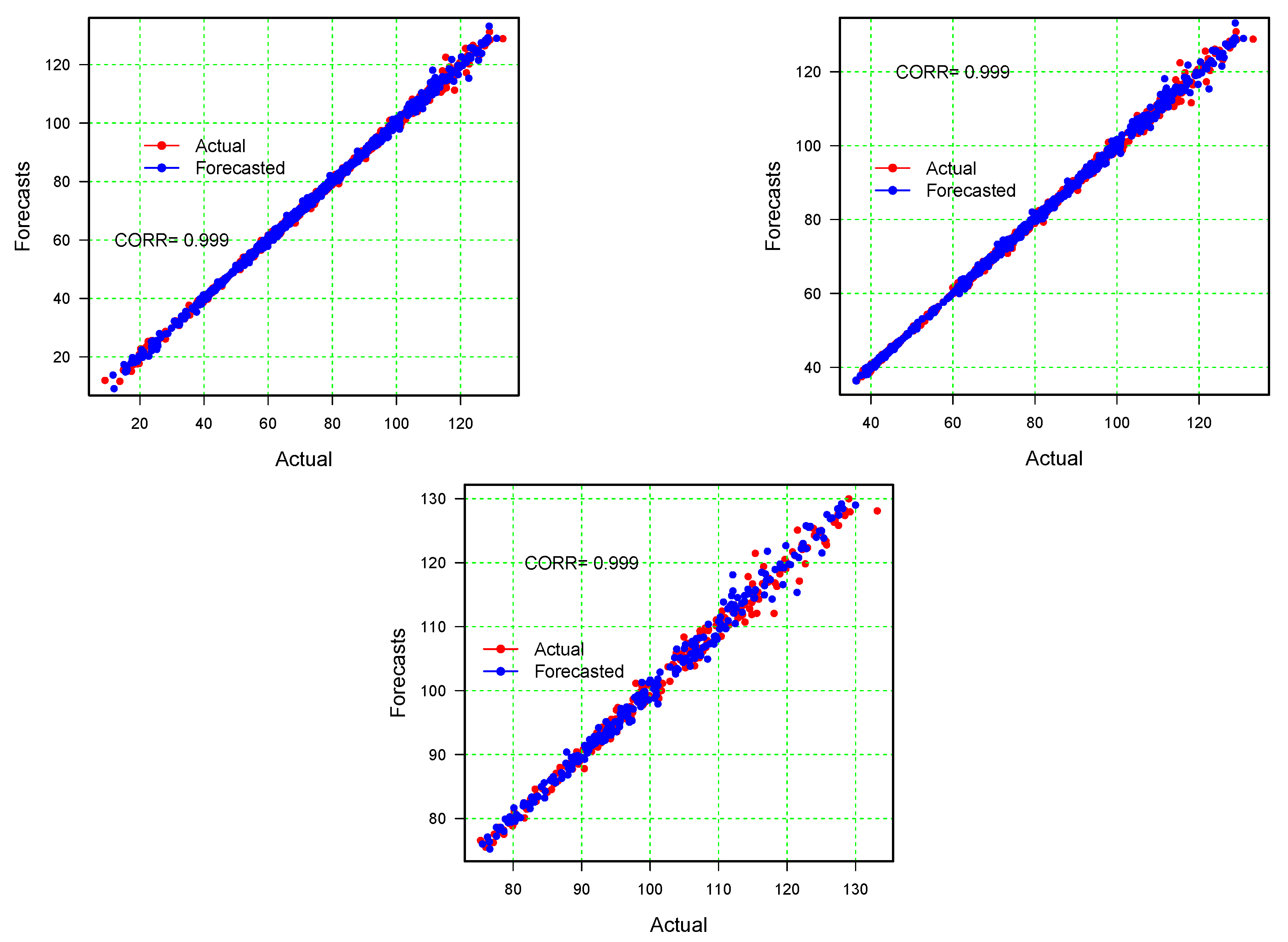In the same way, the correlation plot of the best model (${\mathrm{C}}_3^2$) out of all of the sixteen models in each training and testing scenario is shown in Figure 5: (a) the first scenario results (50%, 50%), (b) the second scenario results (75%, 25%), (c) the third scenario results (90%, 10%). From these figures, it can be seen that the best model (C${}_3^2$) has the greatest correlation coefficient value and shows a significant correlation between the real and forecast values. Finally, at the end of this section, the real and forecast values for the best three combinations of models, C${}_3^4$, C${}_3^4$, and C${}_3^4$, are superimposed on Figure 6; each training and testing scenario is shown in Figure 5: (a) the first scenario results (50%, 50%), (b) the second scenario results (75%, 25%), (c) the third scenario results (90%, 10%). As can be seen in the figure, our model’s forecast follows the original Brent crude oil prices very well. Thus, to conclude this section, from the accuracy metrics (RMSPE, MAPE, MAE, RMSE, CC, and DS), a statistical test (DM test), and graphical outcomes (bar, correlation, and line plots), we can conclude that the proposed hybrid forecasting methodology is highly efficient and accurate for day-ahead Brent crude oil prices. In addition, within the proposed combination of models, the C${}_3^2$ model produced more precise forecasts when compared with the alternative combinations.

4. Discussion

In this section, we discuss the comparison of the proposed best combination model with the considered standard benchmark models, such as the autoregressive, autoregressive moving integrated average, nonparametric autoregressive, and nonlinear neural network models. The details about the comparison are shown as follows; a numerical presentation in

Table 6. Daily spot Brent oil prices: Accuracy measures of the best-proposed combination model versus the benchmark models.

S. No	Model	RMSPE	MAPE	MAE	RMSE	CC	DS
50%, 50%
1	${\mathrm{C}}_3^2$	0.5435	0.8808	0.0171	0.8196	0.9993	0.9280
2	AR	0.6951	1.1221	0.0221	1.0193	0.9988	0.9059
3	ARIMA	0.7121	1.1984	0.0276	1.0572	0.9987	0.9059
4	NPAR	0.5719	0.9237	0.0173	0.8509	0.9992	0.9161
5	NNA	0.7195	1.1719	0.0253	1.0527	0.9988	0.9074
75%, 25%
1	${\mathrm{C}}_3^2$	0.6132	0.7573	0.0104	0.9523	0.9992	0.9364
2	AR	0.8003	0.9890	0.0134	1.1934	0.9988	0.9126
3	ARIMA	0.8082	1.0026	0.0136	1.2031	0.9987	0.9173
4	NPAR	0.6537	0.8073	0.0110	0.9996	0.9991	0.9205
5	NNA	0.8323	1.0247	0.0137	1.2273	0.9987	0.9173
90%, 10%
1	${\mathrm{C}}_3^2$	0.9299	0.8969	0.0122	1.3248	0.9953	0.9518
2	AR	1.2105	1.1767	0.0155	1.6614	0.9925	0.9478
3	ARIMA	1.2197	1.1874	0.0157	1.6688	0.9925	0.9558
4	NPAR	0.9944	0.9639	0.0130	1.4008	0.9947	0.9317
5	NNA	1.2712	1.2379	0.0161	1.7052	0.9921	0.9438

and a graphical presentation in Figure 7. From both presentations, it can be seen that the best model proposed in this work produced comparatively accurate and efficient forecasts for the one-day-ahead Brent crude oil prices. The best-proposed combination model obtained the lowest accuracy measures (RMSPE, MAPE, MAE, and RMSE) and the highest values of CC and DS in all scenarios of training and testing sets, which are significantly better than all of the considered benchmark models in all three training and testing data samples. On the other hand, to confirm the superiority of the proposed best model mentioned in Table 6, we performed a statistical test using the DM on each pair of models. The results (p-values) of the DM test are reported in

Table 7. The best-proposed combination model versus the benchmark models: Results (p-value) of the DM test for the null hypothesis that the two models in the rows and columns are equally accurate and the alternative hypothesis that the model in the column is more accurate than the model in the row.

50%, 50%
Models	${\mathrm{C}}_3^2$	AR	ARIMA	NPAR	NNA
${\mathrm{C}}_3^2$	0.00	1.00	1.00	0.92	1.00
AR	0.00	0.00	0.98	0.00	0.97
ARIMA	0.00	0.02	0.00	0.00	0.39
NPAR	0.08	1.00	1.00	0.00	1.00
NNA	0.00	0.03	0.61	0.00	0.00
75%, 25%
Models	${\mathrm{C}}_3^2$	AR	ARIMA	NPAR	NNA
${\mathrm{C}}_3^2$	0.00	1.00	1.00	0.91	1.00
AR	0.00	0.00	0.77	0.00	0.92
ARIMA	0.00	0.23	0.00	0.00	0.88
NPAR	0.09	1.00	1.00	0.00	1.00
NNA	0.00	0.08	0.12	0.00	0.00
90%, 10%
Models	${\mathrm{C}}_3^2$	AR	ARIMA	NPAR	NNA
${\mathrm{C}}_3^2$	0.00	1.00	1.00	0.95	1.00
AR	0.00	0.00	0.63	0.00	0.86
ARIMA	0.00	0.37	0.00	0.00	0.86
NPAR	0.05	1.00	1.00	0.00	1.00
NNA	0.00	0.14	0.14	0.00	0.00

, showing that among all of the considered benchmark (AR, NPAR, ARMA, and NNA) models, our best combination model outperformed them at the 5% significance level for different combinations of training and testing data. To conclude, based on all of the results, the efficiency and accuracy of the proposed hybrid forecasting technique are comparatively high when compared with all considered competitors.

To sum up this section, crude oil is one of the main energy sources, and its prices have gained increasing attention due to its important role in the world economy. Therefore, accurate prediction of crude oil prices is an important issue not only for ordinary investors but also for the whole of society. To achieve accurate forecasts of nonstationary and nonlinear Brent crude oil price time series, a novel hybrid forecasting technique is developed in this study. Perhaps policymakers, as well as traders, could use the proposed forecasting method when forecasting economic or financial time series data. Our research findings will be of particular interest to investors, traders, regulators, and others. Good forecasts and knowledge of crude oil price trends in developed and developing economies can help traders make more profitable business and trading plans and make useful asset allocation decisions. In addition, based on the best-proposed model, a more robust trading plan can be developed, and the model with the best risk–reward combination can be chosen.

5. Conclusions

Crude oil price forecasting is an important research area in the international bulk commodity market. However, the properties of the time series of daily crude oil prices are complex, being nonstationary and nonlinear, which makes it challenging to produce accurate forecasts. Aiming at bridging that gap, this research work proposed a new hybrid forecasting methodology for daily Brent oil spot prices in which we split the time series of Brent spot prices into two subseries, the long-term nonlinear trend and a stochastic (residual) series, using the Hodrick–Prescott filter. To forecast the two subseries, we also considered two linear and two nonlinear time series models. The proposed modeling framework was applied and evaluated with daily Brent spot prices from 1 January 2013 to 23 December 2022. Six different accuracy measures, pictorial analysis, and statistical tests were performed across different combinations of training and testing data, i.e., (50%, 50%), (75%, 25%), and (90%, 10%). For each of these three scenarios, the model C${}_3^2$ was found to be the best-proposed combination model because it resulted in lower accuracy measures and larger values for CC and DS. However, C${}_3^1$ and C${}_3^3$ were found to be good competitors. After that, we compared the best-proposed combination model to the benchmark models (AR, ARIMA, NPAR, and NNA) by using different accuracy measures and the $DM$ test, showing that the proposed model outperformed the other models.

In conclusion, this study focused specifically on the daily Brent oil price dataset, but the proposed hybrid forecasting technique can be extended to other markets, such as West Texas Intermediate, Dubai Crude Oil, Oman Crude Oil Futures, and more, to evaluate its performance in diverse contexts. By incorporating additional combinations of time series and machine learning models, such as generalized autoregressive conditional heteroskedasticity, support vector machines, decision trees, random forests, short-term memory networks, and other advanced techniques, future research can broaden the range of forecasting approaches and potentially enhance the accuracy and applicability of the proposed methodology. Moreover, only the HP filter was used in this work. In the future, it should be extended to include other filters and check the performance of different filters within the proposed hybrid time series combination models, for example, Hamilton’s filter, exponential moving filter, nonparametric regression filters, etc. In addition, the proposed hybrid forecasting model’s consistency can be assessed using two-day-ahead, three-day-ahead, five-day-ahead, etc., forecasting in future work.

Furthermore, the findings of this study indicate that the proposed combination model outperformed other methods in capturing the complex and nonlinear behavior of crude oil prices. This suggests that the hybrid forecasting approach holds promise for applications beyond crude oil prices (for example, energy [47,48], air pollution [49,50,51], solid waste [52], academic performance [53] and digital marketing [54]). Therefore, it is recommended to employ this methodology for forecasting other complex financial time series data, such as inflation, unemployment, and cryptocurrencies. The demonstrated ability of the hybrid model to deliver highly efficient and accurate forecasts in such scenarios can provide valuable insights into various financial domains.

References

1. Ahmad, W.; Aamir, M.; Khalil, U.; Ishaq, M.; Iqbal, N.; Khan, M.T. A New Approach for Forecasting Crude Oil Prices Using Median Ensemble Empirical Mode Decomposition and Group Method of Data Handling. Math. Probl. Eng. 2021, 2021, 5589717. [Google Scholar] [CrossRef]
2. Wang, J.; Niu, T.; Du, P.; Yang, W. Ensemble probabilistic prediction approach for modeling uncertainty in crude oil price. Appl. Soft Comput. 2020, 95, 106509. [Google Scholar] [CrossRef]
3. Ding, Y.; He, D.; Wu, J.; Xu, X. Crude Oil Spot Price Forecasting Using Ivanov-Based LASSO Vector Autoregression. Complexity 2022, 2022, 5011174. [Google Scholar] [CrossRef]
4. Wen, X.; Wei, Y.; Huang, D. Measuring contagion between energy market and the stock market during the financial crisis: A copula approach. Energy Econ. 2012, 34, 1435–1446. [Google Scholar] [CrossRef]
5. Heinlein, R.; Legrenzi, G.D.; Mahadeo, S.M. Crude oil and stock markets in the COVID-19 crisis: Evidence from oil exporters and importers. Q. Rev. Econ. Financ. 2021, 82, 223–229. [Google Scholar] [CrossRef]
6. Lang, K.; Auer, B.R. The economic and financial properties of crude oil: A review. N. Am. J. Econ. Financ. 2020, 52, 100914. [Google Scholar] [CrossRef]
7. Zhang, X.; Yu, L.; Wang, S.; Lai, K.K. Estimating the impact of extreme events on crude oil price: An EMD-based event analysis method. Energy Econ. 2009, 31, 768–778. [Google Scholar] [CrossRef]
8. Shah, I.; Iftikhar, H.; Ali, S. Modeling and forecasting electricity demand and prices: A comparison of alternative approaches. J. Math. 2022, 2022, 3581037. [Google Scholar] [CrossRef]
9. Wang, Q.; Wang, H.; Gupta, C.; Rao, A.R.; Khorasgani, H. A Non-linear Function-on-Function Model for Regression with Time Series Data. In Proceedings of the IEEE International Conference on Big Data (Big Data), Atlanta, GA, USA, 10–13 December 2020; pp. 232–239. [Google Scholar]
10. Xiong, J.; Wu, P. An analysis of forecasting model of crude oil demand based on cointegration and vector error correction model (VEC). In Proceedings of the 2008 International Seminar on Business and Information Management, Wuhan, China, 19 December 2008. [Google Scholar]
11. Gülen, S.G. Efficiency in the crude oil futures market. J. Energy Financ. Dev. 1998, 3, 13–21. [Google Scholar] [CrossRef]
12. Lanza, A.; Manera, M.; GiovNANNini, M. Modeling and forecasting cointegrated relationships among heavy oil and product prices. Energy Econ. 2005, 27, 831–848. [Google Scholar] [CrossRef]
13. Drachal, K. Forecasting crude oil real prices with averaging time-varying VAR models. Resour. Policy 2021, 74, 102244. [Google Scholar] [CrossRef]
14. Ahmad, M.I. Modelling and forecasting Oman crude oil prices using Box-Jenkins techniques. Int. J. Trade Glob. Mark. 2012, 5, 24–30. [Google Scholar] [CrossRef]
15. Morana, C. A semiparametric approach to short-term oil price forecasting. Energy Econ. 2001, 23, 325–338. [Google Scholar] [CrossRef]
16. Mohammadi, H.; Su, L. International evidence on crude oil price dynamics: Applications of ARIMA-GARCH models. Energy Econ. 2010, 32, 1001–1008. [Google Scholar] [CrossRef]
17. Hou, A.; Suardi, S. A nonparametric GARCH model of crude oil price return volatility. Energy Econ. 2012, 34, 616–626. [Google Scholar] [CrossRef]
18. Joshi, J. Forecasting and Analysing Oil Price Movements using Linear Regression Model. 2016. Available online: https://ssrn.com/abstract=3889596 (accessed on 2 June 2023).
19. Yu, L.; Wang, S.; Lai, K.K. Forecasting crude oil price with an EMD-based neural network ensemble learning paradigm. Energy Econ. 2008, 30, 2623–2635. [Google Scholar] [CrossRef]
20. Movagharnejad, K.; Mehdizadeh, B.; Banihashemi, M.; Kordkheili, M.S. Forecasting the differences between various commercial oil prices in the Persian Gulf region by neural network. Energy 2011, 36, 3979–3984. [Google Scholar] [CrossRef]
21. Mirmirani, S.; Li, H.C. A comparison of VAR and neural networks with genetic algorithm in forecasting price of oil. In Applications of Artificial Intelligence in Finance and Economics; Binner, J.M., Kendall, G., Chen, S.-H., Eds.; Emerald Group Publishing Limited: Bingley, UK, 2004; pp. 203–223. [Google Scholar]
22. Abdullah, S.N.; Zeng, X. Machine learning approach for crude oil price prediction with Artificial Neural Networks-Quantitative (NANN-Q) model. In Proceedings of the 2010 International Joint Conference on Neural Networks (IJCNN), Barcelona, Spain, 18–23 July 2010. [Google Scholar]
23. Xie, W.; Yu, L.; Xu, S.; Wang, S. A new method for crude oil price forecasting based on support vector machines. In Proceedings of the International Conference on Computational Science, Reading, UK, 28–31 May 2006. [Google Scholar]
24. Wang, S.; Yu, L.; Lai, K.K. A novel hybrid AI system framework for crude oil price forecasting. In Chinese Academy of Sciences Symposium on Data Mining and Knowledge Management; Springer: Berlin/Heidelberg, Germany, 2004; pp. 233–242. [Google Scholar]
25. Wang, S.; Yu, L.; Lai, K.K. Crude oil price forecasting with tei@i methodology. J. Syst. Sci. Complex. 2005, 18, 145. [Google Scholar]
26. Sako, K.; Mpinda, B.N.; Rodrigues, P.C. Neural Networks for Financial Time Series Forecasting. Entropy 2022, 24, 657. [Google Scholar] [CrossRef]
27. Sulandari, W.; Subanar, S.; Lee, M.H.; Rodrigues, P.C. Time series forecasting using singular spectrum analysis, fuzzy systems and neural networks. MethodsX 2020, 7, 101015. [Google Scholar] [CrossRef]
28. Rodrigues, P.C.; Pimentel, J.; Messala, P.; Kazemi, M. Decomposition and forecasting of mutual investment funds using singular spectral analysis. Entropy 2020, 22, 83. [Google Scholar] [CrossRef]
29. Rodrigues, P.C.; Awe, O.O.; Pimentel, J.; Mahmoudv, R. Modelling the behaviour of currency exchange rates with singular spectrum analysis and artificial neural networks. Stats 2020, 3, 137–157. [Google Scholar] [CrossRef]
30. Abdollahi, H.; Ebrahimi, S.B. A new hybrid model for forecasting Brent crude oil price. Energy 2020, 200, 117520. [Google Scholar] [CrossRef]
31. Chen, Z.; Ye, Y.; Li, X. Forecasting China’s crude oil futures volatility: New evidence from the MIDAS-RV model and COVID-19 pandemic. Resour. Policy 2022, 75, 102453. [Google Scholar] [CrossRef] [PubMed]
32. Salisu, A.A.; Gupta, R.; Bouri, E.; Ji, Q. Mixed-frequency forecasting of crude oil volatility based on the information content of global economic conditions. J. Forecast. 2022, 41, 134–157. [Google Scholar] [CrossRef]
33. Muşetescu, R.C.; Grigore, G.E.; Nicolae, S. The Use of GARCH Autoregressive Models in Estimating and Forecasting the Crude Oil Volatility. Eur. J. Interdiscip. Stud. 2022, 14, 13–38. [Google Scholar] [CrossRef]
34. Xing, L.M.; Zhang, Y.J. Forecasting crude oil prices with shrinkage methods: Can nonconvex penalty and Huber loss help? Energy Econ. 2022, 110, 106014. [Google Scholar] [CrossRef]
35. Zhang, Y.; He, M.; Wen, D.; Wang, Y. Forecasting crude oil price returns: Can nonlinearity help? Energy 2023, 262, 125589. [Google Scholar] [CrossRef]
36. Dickey, D.A.; Fuller, W.A. Distribution of the estimators for autoregressive time series with a unit root. J. Am.Stat. Assoc. 1979, 74, 427–431. [Google Scholar]
37. Teraesvirta, T.; Lin, C.F.; Granger, C.W.J. Power of the Neural Network Linearity Test. J. Time Ser. Anal. 1993, 14, 209–220. [Google Scholar] [CrossRef]
38. Brockwell, P.J.; Davis, R.A. Introduction to Time Series and Forecasting; Springer: Berlin/Heidelberg, Germany, 2016. [Google Scholar]
39. Shah, I.; Iftikhar, H.; Ali, S.; Wang, D. Short-term electricity demand forecasting using components estimation technique. Energies 2019, 12, 2532. [Google Scholar] [CrossRef]
40. Shah, I.; Iftikhar, H.; Ali, S. Modeling and forecasting medium-term electricity consumption using component estimation technique. Forecasting 2020, 2, 163–179. [Google Scholar] [CrossRef]
41. Iftikhar, H. Modeling and Forecasting Complex Time Series: A Case of Electricity Demand. Master’s Thesis, Quaidi-Azam University, Islamabad, Pakistan, 2018; pp. 1–94. [Google Scholar]
42. Diebold, F.X.; Mariano, R.S. Comparing predictive accuracy. J. Bus. Econ. Stat. 2002, 20, 134–144. [Google Scholar] [CrossRef]
43. Iftikhar, H.; Bibi, N.; Canas Rodrigues, P.; López-Gonzales, J.L. Multiple Novel Decomposition Techniques for Time Series Forecasting: Application to Monthly Forecasting of Electricity Consumption in Pakistan. Energies 2023, 16, 2579. [Google Scholar] [CrossRef]
44. Iftikhar, H.; Khan, M.; Khan, Z.; Khan, F.; Alshanbari, H.M.; Ahmad, Z. A Comparative Analysis of Machine Learning Models: A Case Study in Predicting Chronic Kidney Disease. Sustainability 2023, 15, 2754. [Google Scholar] [CrossRef]
45. Iftikhar, H.; Khan, M.; Khan, M.S.; Khan, M. Short-Term Forecasting of Monkeypox Cases Using a Novel Filtering and Combining Technique. Diagnostics 2023, 11, 1923. [Google Scholar] [CrossRef]
46. Alshanbari, H.M.; Iftikhar, H.; Khan, F.; Rind, M.; Ahmad, Z.; El-Bagoury, A.A.A.H. On the Implementation of the Artificial Neural Network Approach for Forecasting Different Healthcare Events. Diagnostics 2023, 7, 1310. [Google Scholar] [CrossRef]
47. Gonzales, J.L.; Calili, R.F.; Souza, R.C.; da Silva, F.L.C. Simulation of the energy efficiency auction prices in Brazil. Renew. Energy Power Qual. J. 2016, 1, 574–579. [Google Scholar] [CrossRef]
48. López-Gonzales, J.L.; Souza, R.C.; Da Silva, F.L.C.; Carbo-Bustinza, N.; Ibacache-Pulgar, G.; Calili, R.F. Simulation of the energy efficiency auction prices via the markov chain monte carlo method. Energies 2020, 13, 4544. [Google Scholar] [CrossRef]
49. Carbo-Bustinza, N.; Belmonte, M.; Jimenez, V.; Montalban, P.; Rivera, M.; Martínez, F.G.; Mohamed, M.M.H.; De La Cruz, A.R.H.; da Costa, K.; López-Gonzales, J.L. A machine learning approach to analyse ozone concentration in metropolitan area of Lima, Peru. Sci. Rep. 2022, 12, 22084. [Google Scholar] [CrossRef]
50. da Silva, K.L.S.; López-Gonzales, J.L.; Turpo-Chaparro, J.E.; Tocto-Cano, E.; Rodrigues, P.C. Spatio-temporal visualization and forecasting of PM 10 in the Brazilian state of Minas Gerais. Sci. Rep. 2023, 13, 3269. [Google Scholar] [CrossRef] [PubMed]
51. Jeldes, N.; Ibacache-Pulgar, G.; Marchant, C.; López-Gonzales, J.L. Modeling Air Pollution Using Partially Varying Coefficient Models with Heavy Tails. Mathematics 2022, 10, 3677. [Google Scholar] [CrossRef]
52. Quispe, K.; Martínez, M.; da Costa, K.; Romero Giron, H.; Via y Rada Vittes, J.F.; Mantari Mincami, L.D.; Hadi Mohamed, M.M.; Huamán De La Cruz, A.R.; López-Gonzales, J.L. Solid Waste Management in Peru’s Cities: A Clustering Approach for an Andean District. Appl. Sci. 2023, 13, 1646. [Google Scholar] [CrossRef]
53. Orrego Granados, D.; Ugalde, J.; Salas, R.; Torres, R.; López-Gonzales, J.L. Visual-Predictive Data Analysis Approach for the Academic Performance of Students from a Peruvian University. Appl. Sci. 2022, 12, 11251. [Google Scholar] [CrossRef]
54. Sánchez-Garcés, J.; Soria, J.J.; Turpo-Chaparro, J.E.; Avila-George, H.; López-Gonzales, J.L. Implementing the reconac marketing strategy for the interaction and brand adoption of peruvian university students. Appl. Sci. 2021, 11, 2131. [Google Scholar] [CrossRef]
Figure 1. Daily spot Brent oil prices are filtered by the HP filter. Within the figure, the first panel is the original time series ( B t ) of the Brent oil prices; the second panel is the long-term trend ( n t ) series; and the bottom panel shows the stochastic ( s t ) series.
Mathematics 11 03548 g001
Figure 2. Daily Spot Brent Oil Prices: The first panel is the nonlinear long-term trend ( n t ) series, and the bottom panel shows the difference series of the long-term trend series (diff( n t )).
Mathematics 11 03548 g002
Figure 3. A flowchart of the proposed forecasting methodology.
Mathematics 11 03548 g003
Figure 4. Mean accuracy measures’ bar plots. Day-ahead Brent oil forecast mean errors for all sixteen combination models: In each figure, the MAE (first), the MAPE (second), the RMSPE (third), and the RMSE (fourth). Top left: (50%, 50%) and Top right: (75%, 25%). Bottom: (90%, 10%).
Mathematics 11 03548 g004
Figure 5. Correlation plot for the daily Brent crude oil prices for the best combination model (C 3 2 ) along with the coefficient correlation. Top: (50%, 50%) and (75%, 25%). Bottom: (90%, 10%).
Mathematics 11 03548 g005
Figure 6. The original and forecast daily crude Brent oil prices for the best three combinations of models: C 3 2 (red), C 3 1 (blue), and C 3 3 (green). Top: (50%, 50%), Center: (75%, 25%), and Bottom: (90%, 10%).
Mathematics 11 03548 g006
Figure 7. Comparison plots of accuracy measures: Day-ahead Brent oil forecast mean errors for the best combination model (C 3 2 ) versus considered benchmark models: In each sub-figure, the MAE (top-left; red–square), the MAPE (top-right; purple–star), the RMSPE (bottom-left; green–triangle), and the RMSE (bottom-right; blue–circle). Top: (50%, 50%) and (75%, 25%), Bottom: (90%, 10%).
Mathematics 11 03548 g007