
Security Quantification for Discrete Event Systems Based on the Worth of States


1
School of Computer Science and Engineering, Macau University of Science and Technology, Avenida Wai Long, Taipa, Macau SAR 999078, China
2
Hitachi Building Technology (Guangzhou) Co., Ltd., No. 2 Nanxiang 3rd Road, Guangzhou 510613, China
3
Institute of Systems Engineering, Macau University of Science and Technology, Avenida Wai Long, Taipa, Macau SAR 999078, China
*
Author to whom correspondence should be addressed.
Mathematics 2023, 11(17), 3629; https://0-doi-org.brum.beds.ac.uk/10.3390/math11173629
Submission received: 30 June 2023
/
Revised: 11 August 2023
/
Accepted: 21 August 2023
/
Published: 22 August 2023
(This article belongs to the Special Issue Advanced Mathematical Approaches to Engineering and Computational Problems)
Abstract
:This work addresses the problem of quantifying opacity for discrete event systems. We consider a passive intruder who knows the overall structure of a system but has limited observational capabilities and tries to infer the secret of this system based on the captured information flow. Researchers have developed various approaches to quantify opacity to compensate for the lack of precision of qualitative opacity in describing the degree of security of a system. Most existing works on quantifying opacity study specified probabilistic problems in the framework of probabilistic systems, where the behaviors or states of a system are classified as secret or non-secret. In this work, we quantify opacity by a state-worth function, which associates each state of a system with the worth it carries. To this end, we present a novel category of opacity, called worthy opacity, characterizing whether the worth of information exposed to the outside world during the system’s evolution is below a threshold. We first provide an online approach for verifying worthy opacity using the notion of a run matrix proposed in this research. Then, we investigate a class of systems satisfying the so-called 1-cycle returned property and present a worthy opacity verification algorithm for this class. Finally, an example in the context of smart buildings is provided.
1. Introduction
With global urbanization, cities are growing in size and population, and the proportion of people living in urban areas is expected to grow to 68% by 2050 [1], creating inevitable challenges to urban residents due to limited resources and services. The concept of smart cities has been proposed to efficiently deploy public resources, improve social governance, and promote sustainable urban development. Currently, smart cities are being intensively established around the world; for example, there are already more than 500 in China [2].
Buildings provide the physical space required for people to carry out various social, economic, and cultural activities, and are one of the areas where the Internet of Things (IoT) would make significant impacts [3]. Smart buildings improve the energy efficiency, operational efficiency, security, and comfort of the living or working environment by integrating advanced technologies and systems [4,5]. For example, people use the model predictive control approach for temperature control in smart buildings, reducing operating costs and improving thermal comfort [6,7]. However, IoT devices in smart buildings generate a large amount of data, which can pose many potential threats. Deciding how to analyze the security of smart buildings is becoming an increasingly important issue and has attracted a lot of attention over the past few years [8,9,10].
In this article, we study an information flow security property of great interest: opacity, within the discrete event system (DES) framework, where DES can describe the state transition relationships between events in an IoT, thereby assisting us in understanding and analyzing IoT behavior. Opacity was originally introduced in 2004 for the analysis of cryptographic protocols [11]. Later, it is taken as a general information flow security framework for a DES interacting with a passive intruder. Many kinds of information flow security properties can be formulated as opacity, such as non-interference [12], anonymity [13], etc. Roughly speaking, opacity is a type of confidentiality property that characterizes whether certain secret information from a system can be deduced by outside observers that may be malicious.
In the context of DESs, opacity is classified into language-based and state-based opacity, depending on the defined secret [14]. Language-based opacity has been studied with models such as automata [13] and Petri nets [15], where the secret is defined as a language. In general, this type of opacity can be further classified as strong and weak opacity, as opposed to state-based opacity, which has a wide range of classifications depending on the state of interest. For example, current-state opacity [16,17] has been proposed to take the system’s current state as a secret and determine whether the system reveals this secret during its evolution. Similarly, initial-state opacity [18] and initial-and-final-state opacity [19] are suggested when the secret is defined as a set of initial states or a set of secret state pairs. The notions of K-step opacity [20] and infinite-step opacity [21] are developed when the delayed information of a system is concerned, and pre-opacity [22] is formulated when the intention of a system needs to be kept secret.
All of the aforementioned notions of opacity describe a system in a binary way, where the system is either opaque or non-opaque. It has been noted that qualitative opacity is not accurate enough in assessing the information obtained by passive attackers [23]. For instance, a system that violates qualitative opacity with a very low probability and one that violates qualitative opacity with a very high probability are considered insecure. However, their degree of security is different [24]. The authors of [25] introduce game theory’s ideas into probabilistic automata and propose a model of probabilistic resource automata based on which the current-state opacity is quantified.
The above-mentioned studies on quantification of opacity are basically based on probabilistic systems. However, a probabilistic model is much more difficult to be abstracted than a non-probabilistic version. The study in [26] is the first work that introduces the quantification of opacity into non-probabilistic DES. Considering that the essence of opacity is to explore the observational equivalent strings, the authors developed a method to calculate the opacity degree of a system by computing the dispersion among non-secret runs and secret equivalents.
In this work, we investigate the quantification of opacity from a new perspective by describing the worth of information that each system state carries in terms of a state-worth function. Then, we introduce a new type of opacity, called worthy opacity, to describe whether the worth of information exposed to the outside world in the system’s evolution meets the security requirements. We consider an intruder who knows the whole structure of a system but has limited observation capabilities. Unlike the general notions of state-based opacity, we do not explicitly treat a secret as a specific sub-set of states since the state-worth function describes the importance of each system state. We show that current-state opacity is strictly weaker than worthy opacity. The proposed notion of worthy opacity is closely related to the notion of opacity degree in [26]. The contributions of this article can be summarized as follows:
- A novel notion of worthy opacity is proposed to quantitatively characterize the worth of a system available to an intruder;
- An online algorithm is provided to verify worthy opacity;
- A system property called 1-cycle returned is defined, and an offline verification algorithm for the system’s worthy opacity satisfying this property is presented;
- It is shown that worthy opacity provides a more granular partitioning of the system than current-state opacity.
2. Preliminaries
Symbols , , , and are specified to denote the sets of real numbers, non-negative real numbers, non-negative integers, and positive integers, respectively. The ceiling function of a real number , denoted as , is defined as the smallest integer that is not smaller than x. For a vector , is used to denote the i-th entry of . Given a matrix , its -th entry is denoted as . The transpose of a vector is denoted by . Given a k-dimensional vector , its 1-norm is defined as the sum of the absolute values of each entry, i.e., . The L1-normalization of a vector , denoted by in this article, is defined as . Given an ordered pair , we use and to denote its first and second components, namely, and .
2.1. System Model
We define an alphabet as any non-empty finite set of events, denoted by E. A string over the alphabet E is a sequence of events taken out of E [27]. The length of a string s, written as (if X is a set, the notation denotes the cardinality of X. The distinction is usually clear from context), is the number of events contained in it, counting multiple occurrences of the same event. The string without any events is called the empty string and is denoted by with . Given two strings and , the concatenation of and is the sequence of events in followed by the sequence of events in , denoted as or . We use the superscript notation to indicate that the string s is concatenated with itself k times.
Given an alphabet E, we denote by the set of all strings of length k, particularly, . The set consisting of all finite-length strings defined over E is denoted by , i.e., . Given an alphabet E, a language is a sub-set of . Given two languages and , the concatenation of and is . In this article, we model a DES as a non-deterministic finite automaton, formally defined as follows.
Definition 1
(Non-deterministic Finite Automaton). A non-deterministic finite automaton (NFA) is a four-tuple , where
- is the finite set of states;
- is the finite set of events associated with G;
- (where is the power set of Q) is the transition function, and means that there is a transition labeled by e from state q to state ;
- is the set of initial states.
If in G is a singleton and the transition function of G is a partially defined function , then G is called a deterministic finite automaton (DFA). The transition function f can be extended recursively from the domain to the domain : and for all states , where and . The language generated by G from state is , where indicates that is defined, i.e., . The language generated by G from a set of states is . Naturally, the language generated by G is .
Formally an NFA G can be equivalently represented by a directed graph, with a set of nodes Q denoting states and a set of edges denoting transitions. A run in G starting from is a finite sequence of transitions (here, we use the numbers in parentheses to indicate the order in which states or events appear in the run, that is to say, is not necessarily equal to and is not necessarily equal to ), and the events extracted from it in order form the string associated with it, denoted by (we also say that r is a run on and use to denote the ending state). We define the length of a run r as the length of the string associated with it, i.e., . Given a run from state q to on a string s, we denote it as ; if a specific string associated with the run is not of interest, we denote it as . The set of all runs starting from state in G is denoted by ; the set of all runs generated by G is . A run of length greater than zero that begins and ends at the same state is called a cycle.
2.2. Intruder Model and Opacity
In the general setting of studying opacity in DESs, it is assumed that the intruder is fully aware of the system’s structure but only partially observes the system’s behavior [14]. We follow this setting in our work and formalize it as the partial observability of events, where the set of events E is divided into an observable event set and an unobservable event set , i.e., . Given a string generated by G, the intruder’s observation is the output of the natural projection function , which is defined recursively as:
The unobservable reach of a state in G, denoted by , is . This definition can be extended to a set of states by .
This work is an extension of state-based opacity, where the secret of a system is a sub-set of states . When a system generates a string , the intruder observes and infers whether the system is in a secret state based on this observation and the system’s structure.
Definition 2
(Current-State Opacity [14]). Given a system , a secret , and a set of observable events , G is current-state opaque with respect to S and , written as -CSO, if
In plain words, a system being current-state opaque means that an intruder cannot infer whether the current state belongs to the secret, regardless of the sequence of events occurring in the system. Given an observation , the current-state estimate associated with is , and the set of consistent strings is .
Lemma 1
([28]). Given a system , a secret , and a set of observable events , G is -CSO if and only if for any observation , .
By Lemma 1, to verify current-state opacity, we can construct the observer of system G and check whether there exists a state in observer that is a sub-set of S [16].
Definition 3.
Given a system and a set of observable events , its observer is a DFA , where
- , with each state being a state estimate generated by an intruder based on the evolution of G;
- is the set of events that can be observed by an intruder;
- ;
- is the initial state estimate.
2.3. Some Counting Principles
As an essential part of combinatorics, counting objects with specific properties is indispensable for the study of DESs. Many different types of problems require us to count items. For instance, some notions of diagnosability are defined in terms of fault counting problems [29]. Counting is also required to determine the complexity of algorithms [30]. In addition, counting techniques are widely used in calculating the finite probability [31]. Our work is also inseparable from counting. This subsection recalls some critical counting principles [32].
Lemma 2
(Addition Principle). Suppose that a set S can be partitioned into pairwise disjoint parts . The number of elements in S is the sum of the number of elements in each of its part, i.e., .
We divide the problem into mutually exclusive cases for applying the addition principle. An alternative formulation of Lemma 2 is as follows: if there are m ways to complete a task, where the i-th way has () choices, then there are choices for completing that task.
Example 2.
Consider the system in Example 1. Suppose we want to find the number of cycles of length two in . We divide these cycles by listing their start and end states. The number of 2-length cycles starting and ending in states , , , and are 2, 2, 1, and 1, respectively. Therefore, the number of cycles of length two in is .
Lemma 3
(Multiplication Principle). Let S be a set of m-tuples , where the i-th component comes from a set of size . The size of S is .
The multiplication principle is a corollary of Lemma 2. A useful formulation of Lemma 3 is as follows: suppose that a task can be decomposed into m consecutive steps. If step i can be performed in ways, and for each of these, step can be performed in () ways, then the task itself can be accomplished in ways.
Example 3.
Consider the system in Example 1. The number of 2-length runs starting from state , passing through state , and ending at state is 1, as the number of 1-length runs from state to and state to is 1, respectively.
Lemma 4
(Generalized Pigeonhole Principle [33]). If p objects are placed into q boxes, then at least one box contains a minimum of objects.
3. Notions of Worthy Opacity
In this section, we first provide the definition of worthy opacity for DESs, and then compare it with the widely studied current-state opacity. Existing notions of state-based opacity, both qualitative and quantitative, divide the set of states into secret or non-secret. However, various degrees of confidentiality exist for different states that are part of the same secret. For example, a spy trying to hide his/her tracks would wish neither his/her hiding place be exposed nor the convenience store he/she regularly visits be discovered. Nevertheless, it is clear that the secrecy of the hiding place is more valuable. To describe the degree of confidentiality of individual states, we introduce the notion of state-worth function.
Definition 4
(State-worth Function). Given a system , a state-worth function is a mapping that assigns a non-negative number to a state, defined as .
Note that instead of describing the degree of confidentiality of each state in the secret (a sub-set of the state set), we define the state-worth function as assigning a worth to each state of the system. This is a more general approach than splitting the states into two categories. When linked to the conventional notion of secret, we can use this function to divide secrets: each state possesses a worth, and states carrying worth above a certain threshold are considered constituent elements of a secret.
Example 4.
Suppose that we have a bank account with a deposit limit of $300 and a balance of $100. The amount we deposit into our account or spend at a point of sale (POS) is $100 each time. In addition, a private detective is lying in wait at the bank door and wants to know our financial situation, and he can only find out that we deposit but not that we use POS spending.
Then, the above scenario can be modeled with the system of Example 1; event represents the deposit of $100 while event represents the POS spending of $100. Each state represents the balance of the bank account, and naturally, we can take the balance represented by each state as the value of the state-worth function, i.e., , , , and . If we treat a bank balance over $100 as a secret, then it is , as shown in Example 1.
In addition, the existing notions of opacity are not sufficiently refined for depicting the evolution of a system. In fact, the most fundamental element of a system corresponding to an observation is the set of runs rather than the set of strings, as shown in Figure 2. Specifically, given a run of a system G, we can obtain the string by extracting the sequence of events occurring in it, also commonly considered as the logical behavior of a system, and then an intruder obtains the corresponding observation based on the observability of the events.
Definition 5.
Given a system with a set of observable events and an observation , the set of consistent runs and the set of consistent runs ending in state are defined as and , respectively.
Intuitively, given an observation , the set of consistent runs is the set of all runs for which the system can generate that observation, and accordingly, the set is the set of all runs that cause the system to produce that observation and reach state q.
Definition 6
(Worthy Opacity). Given a system with state-worth function Δ, a set of observable events , and a non-negative value , an observation is worthy opaque with respect to , Δ, and K (denoted by -WO) if
where . System G is said to be worthy opaque with respect to , Δ, and K (-WO) if all observations are -WO.
Note that in Definition 6 can be viewed as the intruder’s probability estimate of the current state of the system as q after observing , i.e., the probability of system G in state when observation is generated is implicitly defined as the number of runs in which the system generates observation and ends up in state q divided by the number of all runs that can generate observation . Then, the left-hand side of (1) shows the worth the system is expected to expose for generating the observation . That is to say, a system is worthy opaque if the worth it exposes to the outside world during its evolution does not exceed a certain threshold.
Example 5.
Consider the situation in Example 4, which is modeled as the system of Example 1. Suppose that the private detective sees that we deposit $100 in the bank, i.e., the system produces the observation . We have . Thus, we have , , , and , leading to , , and . By (1), we have , implying that observation is -WO. In plain words, the worth of information revealed to the outside world by observation is 80, which is a reasonable inference that the private detective can make.
Notice that the probabilities implied in Definition 6 are based on a uniform distribution over the set of consistent runs, which implies that the set must be finite, since there is no uniform distribution over infinite countable sets; otherwise the additivity of the probability axioms [31] is violated. Therefore, we have the following assumption on system G.
Assumption 1.
There are no unobservable cycles in the system G, where an unobservable cycle is a cycle such that .
The above assumption ensures that, for each observation, the set of consistent runs is finite (as shown in Proposition 1), and this assumption is also a general one when the system is modeled as a Petri net and the problem is analyzed using the notion of a basis reachability graph [28].
Proposition 1.
Given a system with a set of observable events , the set is finite for any observation if there are no unobservable cycles in G.
Proof.
We first show that system G can generate no more than runs of length k, where N is the number of states and M is the number of events in G. Note that we can consider a k-length run as a cross-arrangement of states and k events, provided that the transition function f is satisfied and . The number of k-length runs is maximized by setting and (for any and ). In this way, each state and each event in a run can be arbitrarily selected from N states and M events, respectively. In other words, the number of k-length runs cannot exceed .
Then, we prove the proposition by contrapositive. Suppose that there exists an observation such that the set is infinite. The length of runs in set can be greater than any given positive integer L. Otherwise, the number of runs in cannot exceed , which implies that is finite.
Now, let , we can find a run
whose length is greater than L. By Lemma 4, we can obtain that there is a state of G that is duplicated at least times in . This implies that there are at least cycles in that begin and end with state . Since the length of is , we conclude that at least one of these cycles is unobservable, which completes the proof. □
Recall that in the research of state-based opacity, the secret is defined as a sub-set of system states. In general, secret states are more valuable than non-secret states. With this consideration, we can relate current-state opacity to the proposed worthy opacity.
Proposition 2.
Given a system with state-worth function Δ, a secret (), and a set of observable events , G is -CSO, if G is -WO.
Proof.
By contrapositive, suppose that G is not -CSO. By Lemma 1, there exists an observation such that . That is, for any , holds, which leads to the fact that G is not -WO. □
Note that the converse of the above proposition does not hold, as illustrated by the following example.
4. Verifying Worthy Opacity
Intuitively, to verify the worthy opacity of a given system G, we need to check whether (1) holds for all , which means that the value of needs to be computed for all . In general, this requires an exhaustive enumeration of all possible strings that can be generated by G, which may require infinite memory and thus render the problem unsolvable. In this section, we first provide an online verification procedure, and then propose an algorithm to identify a particular class of systems and verify their worthy opacity.
4.1. Online Verification of an Observation
Given an observation , we develop a notion of run matrix to compute the cardinality of a set (for any ) based on the transition matrix of automata.
Definition 7
(Transition Matrix [34]). Given an event of a system , the transition matrix is an matrix, where the typical entry is equal to one if and to zero otherwise.
Example 7.
Consider the system in Example 1. The transition matrices associated with events and are, respectively:
As runs are composed of transitions, we can utilize the transition matrix to calculate the number of runs between two states on a given string . Based on the idea of a transition matrix, we propose the notion of a run matrix.
Definition 8
(Run Matrix). Given a system and a string , the run matrix is an matrix whose typical entry is equal to the number of runs from to on string s.
Recall that the values of transition function f of system G are sub-sets of states rather than multi-sets [35], which means that given a state q and an event e, the number of runs from state q to on the one-length string e is one if and zero otherwise. This coincides with the definition of the transition matrix; hence, for all . For the empty string , to fit the extended definition of transition function, we have , where is an identity matrix of size N.
Remark 1.
For a string , its corresponding run matrix is a null matrix, indicating no run on s in G from whatever state it starts in.
Even though we specify the run matrices associated with strings of length zero and one for a given system G, it is still a problem to compute the run matrix associated with a string s of length greater than one, which is a more general case. Before we introduce the computation, we prove the following two properties of run matrices.
Proposition 3.
Given two strings and that have corresponding run matrices and , respectively,
- (1)
- In the case that and are not identical, the number of runs on string or can be described by matrix , i.e., the number of runs from state to on string or is ;
- (2)
- The number of runs on string can be described by matrix , i.e., the number of runs from state to on string is .
Proof.
(1) As , a system cannot generate strings and simultaneously, whereas the way the system generates a string is the number of runs it can generate on that string. By Lemma 2, we have that the number of runs on string or is equal to the sum of the number of runs on and the number of runs on , which is .
(2) Clearly, a system generates a string in the order that first yields and then generates . By Lemma 3, we have that the number of runs from state to on is equal to the product of the number of runs from state to any state and the number of runs from that state to state , which is . □
Remark 2.
Given any string , we have , which also meets the definition of the concatenation of strings.
Based on the second part of the above proposition, we have the following corollary, which can be used to calculate the run matrix associated with a string of length greater than zero.
Corollary 1.
The run matrix associated with a string () is
We can also extend the notion of run matrices to languages, i.e., given a language L, the run matrix associated with it is an matrix whose typical entry is equal to the total number of runs on all strings in L from to . It is not difficult to conclude that . Moreover, the extended run matrix has the following properties.
Proposition 4.
Given two finite languages and that have corresponding run matrices and , respectively,
- (1)
- In the case that and are disjoint, .
- (2)
- .
Proof.
(1) As and are disjoint, the string in either belongs to or to . Therefore, we have .
(2) By , and the definition of extended run matrices, we have , where the first equal sign is due to the second part of Proposition 3. □
Remark 3.
For any finite language , we have , as for any , we have by Remark 1, where is a null matrix.
Proposition 5.
Given a system , define an N-dimensional column vector π such that if and otherwise. Then, is the total number of runs generated by system G on strings in language L, where the ending state of these runs is .
Proof.
It can be directly obtained from the definition of the multiplication of matrices and the meaning of run matrices. □
Based on the above discussions, we can use matrix operations to calculate the number of runs between different states on observations. It is not difficult to find that given an observation , we have . Based on Definition 5, we know that the cardinality of set is the total number of runs generated by the system on all strings in language that can reach state q, i.e., (). With Remark 3, once the run matrix corresponding to the language ⋯ is obtained, the cardinality of set for any is calculated.
Clearly, for any , we have . The remaining problem is how to determine the run matrix associated with . Considering the set of unobservable events as a language, we have . By the second part of Proposition 4, we have for . Note that by , there is .
Theorem 1.
Given a system with no unobservable cycles, the run matrix associated with is .
Proof.
Since and any two sets in are disjoint, by Proposition 4, we have . Suppose that there exists a run r of length N generated by G with states, where N is the number of states in G. By Lemma 4, we can find a duplicate state in r. This indicates the existence of an unobservable cycle in r, which violates the premise that there are no unobservable cycles in G. Therefore, the length of unobservable runs generated by G cannot be greater than N. Naturally, we have for all . From this, we obtain .
Furthermore, by (3), we conclude that the matrix is invertible and . □
Remark 4.
In the following, we will notate the run matrix associated with as for brevity of notation. If there are no unobservable events in the system G, then , leading to without affecting the results below.
In light of the above discussion, it is natural to present Algorithm 1 for the online verification of worthy opacity. Lines 3 to 8 are the initialization of the marker variable and the count vector , where is set to be to indicate that the system is worthy opaque, and the i-th entry of indicates the number of system-generated runs ending in state , inferred by an intruder from the observation. Lines 9 to 23 are the intruder’s online judgment of worthy opacity, whereas lines 10 to 14 are calculations of the expected worth of the currently revealed information. Once the expected worth exceeds K, which means that the system is not worthy opaque, set the to be and stop observing as shown in lines 15 to 18; otherwise, continue the observation as shown in lines 19 to 22. As regards the complexity of Algorithm 1, we note that the complexity of the recursive step k (observe the kth event) is .
Example 8.
Consider the system in Example 1, where its state-worth function is shown in Example 4. Given an observation , we verify online the -worthy opacity of ω using Algorithm 1. Initially, ω is set to be the empty string, i.e., . By Algorithm 1, we have that the expected worth for this system is 50, which is less than 100, implying that the null observation ε is -WO. Similarly, after observing , the value of becomes , so is also -WO. Continuing to run the algorithm, after observing again, we have , implying that is -WO.
| Algorithm 1 Online verification of worthy opacity |
|
4.2. Run Status Recorder and 1-Cycle Returned
It is not difficult to find that for any observation , there is if , which leads to if , and implies that we can narrow the computation from to . We call the set the current-state probability distribution estimate associated with , denoted by . Note that the observer mentioned in Definition 3 represents, in a compact structure, all possible current state estimates during the evolution of a system. Inspired by this idea, it seems that we can also represent all current-state probability distribution estimates in a finite structure. Unfortunately, as the system evolves, there may be an infinite number of sets , as the sets and do not correspond one-to-one.
By analyzing the evolution of a system, we find that if there is no cycle in its observer. Then, the observations generated by that system are finite, which means that the number of set is also finite. Thus, the verification of worthy opacity can be achieved by traversing all observations to determine whether (1) holds. In contrast, if there is a cycle in the observer of a system, then this system can generate an infinite number of observations.
Given a cycle of an observer, the system associated with that observer can generate an infinite number of observations of the form (), assuming that the observation when the observer first enters the cycle is . If , we say that the cycle is 1-cycle returned (1-CR), and if all cycles in an observer of a system are 1-CR, then we say that this system is 1-CR. Fortunately, if a system G is 1-CR, then the current-state probability distribution estimate that can be generated by G is finite, i.e., the worthy opacity of system G is verifiable, as shown in Example 6.
Given a system G, we check whether G is 1-CR by Algorithm 2 and, if so, construct a run status recorder, which is an automaton that enumerates all possible current-state probability distribution estimates generated by system G (see Figure 4). The core idea of Algorithm 2 comes from Proposition 6.
Proposition 6.
Given two N-dimensional column vectors and that satisfy , for any matrix , it holds that .
Proof.
Let . We have and , where and are 1-norms of and , respectively. Hence, one obtains
This completes the proof. □
| Algorithm 2 Construction of the run status recorder and and verification of the 1-CR of system G |
|
Each state in the run status recorder is an ordered pair of two vectors, whose first component is the count vector mentioned in Algorithm 1, denoting the number of runs that reach each state after the system generates a certain observation. Its second component is the L1-normalization of the first vector. Proposition 6 shows that we can merge count vectors that have the same L1-normalization because we are only interested in the current-state probability distribution estimates, which is why we use the second component of the state to identify the different states.
Algorithm 2 works as follows: Lines 3 to 11 are the initialization of the key parameters of the algorithm, where set includes all possible current-state probability distribution estimates generated by the input system and set contains the states generated by the algorithm for which subsequent states are not computed. Function in line 16 of Algorithm 2 is defined as if otherwise , representing a current-state estimate of system G. Once the judgment condition in line 16 is satisfied, it means that the newly generated current-state probability distribution estimate, which different from some previously calculated current-state probability distribution estimate, corresponds to the same current-state estimate, i.e., this system is not 1-CR.
The construction of a run status recorder shows that the number of its states is related to the number of cycles in the observer of the input system G. The number of cycles in an observer of system G containing i different states is , where the observer is considered as the worst case. Then, these cycles can produce different states in in the worst case. Therefore, the complexity of Algorithm 2 is . Although the complexity of Algorithm 2 looks formidable, there are few systems that can reach the worst case that we analyze. If there is no cycle in the observer of a system, then the complexity of Algorithm 2 is reduced to .
Theorem 2.
Given a system with state-worth function Δ, a set of observable events , and a non-negative value , if system G is 1-CR, then construct the run status recorder as in Algorithm 2. System G is worthy opaque with respect to , Δ and K if and only if for any states , holds, where Δ is an N-dimensional row vector with .
Proof.
(Sufficiency) By contrapositive, assume that there exists a state y in such that . Let be the observation that leads to y from . By the construction of , we have that, for the observation , holds. By Definition 6, G is not worthy opaque with respect to , and K.
(Necessity) Also by contrapositive, assume that G is not worthy opaque with respect to , and K. By Definition 6, there exists an observation such that . By the construction of , we conclude that there is a state with . □
Example 9.
Consider a single-story smart building with five rooms marked with , , , , and , as shown in Figure 5a. A bi-directional door exists between and , and , and , and , while to have a uni-directional door. And these five rooms are provided to three different departments according to and , and , and . A smart vehicle provides different services to staff depending on the department, with sensors inside the vehicle that identify the current department. Five levels of confidential documents need to be stored in these five rooms, ranging in value from 1 to 5. Now, suppose that an intruder can read the sensor data of a smart vehicle; how does one allot the five rooms to store confidential documents such as to minimize the worth of information exposed by the vehicle?
The vehicle’s trajectory can be represented by the model shown in Figure 5b. The five states to correspond to the five rooms to , respectively. Events to represent the sensor readings of the vehicle reaching each room, respectively. Since the intruder does not know the exact location of the vehicle but can obtain the sensor readings, the initial state of this model is and the observable event set is . Now, running Algorithm 2 with system as input, we can obtain the corresponding run status recorder as shown in Figure 6.
By assumption, the state-worth function Δ of system is a one-to-one mapping from Q to . Let Δ be an N-dimensional row vector with . Then, the problem of allotting the rooms where the confidential documents are to be stored is transformed into how to define the function Δ such that the maximum value in is minimized. Based on states , , and , we know that the two documents with the highest level of confidentiality can only be placed in rooms and , respectively. Once this is done, it is not difficult to verify that , which means the system is -WO.
In plain words, we only need to place the documents with the highest and second-highest level of confidentiality in rooms and , respectively; then, no matter how the sensor data of the vehicle is exposed, the worth of the information it reveals to the outside world will not exceed 3.
5. Conclusions
In this article, we introduce a notion of worthy opacity to quantify the worth of information released by a partially observed DES modeled with an automaton. We propose an online verification algorithm that considers an intruder who waits and observes the occurrence of observable events and determines whether the observation is worthy opaque. We also present a 1-CR system to verify the worthy opacity offline.
We believe that there are multiple interesting directions for future work related to the notion of worthy opacity. An attractive direction is to synthesize a supervisor that enforces worthy opacity when the verification result is negative. Also, we would like to apply the notion of worthy opacity to more complex, realistic environments.
Author Contributions
Conceptualization, S.Z. and L.Y.; methodology, S.Z.; software, S.Z.; validation, J.Y. and L.Y.; formal analysis, Z.L.; investigation, J.Y.; resources, Z.L.; writing— original draft preparation, S.Z.; writing—review and editing, Z.L.; visualization, S.Z.; supervision, L.Y.; project administration, L.Y. and Z.L.; funding acquisition, L.Y. and Z.L. All authors have read and agreed to the published version of the manuscript.
Funding
This research was funded by the Guangzhou Innovation and Entrepreneurship Leading Team Project Funding under grant No. 202009020008 and the Science and Technology Fund, FDCT, Macau SAR, under grant No. 0101/2022/A.
Data Availability Statement
No new data were created or analyzed in this study. Data sharing is not applicable to this article.
Conflicts of Interest
The authors declare no conflict of interest.
Abbreviations
The following abbreviations are used in this manuscript:
| DES | Discrete Event System |
| DFA | Deterministic Finite Automaton |
| IoT | Internet of Things |
| NFA | Non-deterministic Finite Automaton |
| 1-CR | 1-Cycle Returned |
References
- Khor, N.; Arimah, B.; Otieno, R.; Oostrum, M.; Mutinda, M.; Martins, J. World Cities Report 2022: Envisaging the Future of Cities. 2022. Available online: https://unhabitat.org/sites/default/files/2022/06/wcr_2022.pdf (accessed on 29 June 2022).
- Yang, J.; Lee, T.Y.; Zhang, W. Smart cities in China: A brief overview. IT Prof. 2021, 23, 89–94. [Google Scholar] [CrossRef]
- Jia, M.; Komeily, A.; Wang, Y.; Srinivasan, R.S. Adopting Internet of Things for the development of smart buildings: A review of enabling technologies and applications. Autom. Constr. 2019, 101, 111–126. [Google Scholar] [CrossRef]
- Verma, A.; Prakash, S.; Srivastava, V.; Kumar, A.; Mukhopadhyay, S.C. Sensing, controlling, and IoT infrastructure in smart building: A Review. IEEE Sens. J. 2019, 19, 9036–9046. [Google Scholar] [CrossRef]
- Shaikh, P.H.; Nor, N.B.M.; Nallagownden, P.; Elamvazuthi, I.; Ibrahim, T. A review on optimized control systems for building energy and comfort management of smart sustainable buildings. Renew. Sustain. Energy Rev. 2014, 34, 409–429. [Google Scholar] [CrossRef]
- Carli, R.; Cavone, G.; Dotoli, M.; Epicoco, N.; Scarabaggio, P. Model predictive control for thermal comfort optimization in building energy management systems. In Proceedings of the 2019 IEEE International Conference on Systems, Man and Cybernetics (SMC), Bari, Italy, 6–9 October 2019; pp. 2608–2613. [Google Scholar]
- Ascione, F.; Bianco, N.; De Stasio, C.; Mauro, G.M.; Vanoli, G.P. Simulation-based model predictive control by the multi-objective optimization of building energy performance and thermal comfort. Energy Build. 2016, 111, 131–144. [Google Scholar] [CrossRef]
- Komninos, N.; Philippou, E.; Pitsillides, A. Survey in smart grid and smart home security: Issues, challenges and countermeasures. IEEE Commun. Surv. Tutor. 2014, 16, 1933–1954. [Google Scholar] [CrossRef]
- Wendzel, S. How to increase the security of smart buildings? Commun. ACM 2016, 59, 47–49. [Google Scholar] [CrossRef]
- Hu, J.; Zhang, Z.; Lu, J.; Yu, J.; Cao, J. Demand response control of smart buildings integrated with security interconnection. IEEE Trans. Cloud Comput. 2022, 10, 43–55. [Google Scholar] [CrossRef]
- Mazaré, L. Using unification for opacity properties. In Proceedings of the 4th IFIP WG 1.7, ACM SIGPLAN and GI FoMSESS Workshop on Issues in the Theory of Security, Barcelona, Spain, 3–4 April 2004. [Google Scholar]
- Bryans, J.; Koutny, M.; Mazaré, L.; Ryan, P. Opacity generalised to transition systems. Int. J. Inf. Secur. 2008, 7, 421–435. [Google Scholar] [CrossRef]
- Lin, F. Opacity of discrete event systems and its applications. Automatica 2011, 47, 496–503. [Google Scholar] [CrossRef]
- Jacob, R.; Lesage, J.J.; Faure, J.M. Overview of discrete event systems opacity: Models, validation, and quantification. Annu. Rev. Control 2016, 41, 135–146. [Google Scholar] [CrossRef]
- Tong, Y.; Ma, Z.; Li, Z.; Seatzu, C.; Giua, A. Verification of language-based opacity in Petri nets using verifier. In Proceedings of the 2016 American Control Conference, Boston, MA, USA, 6–8 July 2016. [Google Scholar]
- Saboori, A.; Hadjicostis, C.N. Notions of security and opacity in discrete event systems. In Proceedings of the 46th IEEE Conference on Decision and Control, New Orleans, LA, USA, 12–14 December 2007. [Google Scholar]
- Dong, Y.; Li, Z.; Wu, N. Symbolic verification of current-state opacity of discrete event systems using Petri nets. IEEE Trans. Syst. Man Cybern. Syst. 2022, 52, 7628–7641. [Google Scholar] [CrossRef]
- Saboori, A.; Hadjicostis, C.N. Verification of initial-state opacity in security applications of discrete event systems. Inf. Sci. 2013, 246, 115–132. [Google Scholar] [CrossRef]
- Wu, Y.C.; Lafortune, S. Comparative analysis of related notions of opacity in centralized and coordinated architectures. Discret. Event Dyn. Syst. 2013, 23, 307–339. [Google Scholar] [CrossRef]
- Saboori, A.; Hadjicostis, C.N. Verification of K-step opacity and analysis of its complexity. IEEE Trans. Autom. Sci. Eng. 2011, 8, 549–559. [Google Scholar] [CrossRef]
- Saboori, A.; Hadjicostis, C.N. Verification of infinite-step opacity and complexity considerations. IEEE Trans. Autom. Control 2011, 57, 1265–1269. [Google Scholar] [CrossRef]
- Yang, S.; Yin, X. Secure Your Intention: On Notions of Pre-Opacity in Discrete-Event Systems. IEEE Trans. Autom. Control 2023, 68, 4754–4766. [Google Scholar] [CrossRef]
- Bérard, B.; Mullins, J.; Sassolas, M. Quantifying opacity. Math. Struct. Comput. Sci. 2015, 25, 361–403. [Google Scholar] [CrossRef]
- Saboori, A.; Hadjicostis, C.N. Current-state opacity formulations in probabilistic finite automata. IEEE Trans. Autom. Control 2014, 59, 120–133. [Google Scholar] [CrossRef]
- Li, D.; Yin, L.; Wang, J.; Wu, N. Game current-state opacity formulation in probabilistic resource automata. Inf. Sci. 2022, 613, 96–113. [Google Scholar] [CrossRef]
- Bourouis, A.; Klai, K.; Hadj-Alouane, N.B. Measuring opacity for non-probabilistic DES: A SOG-based approach. In Proceedings of the 24th International Conference on Engineering of Complex Computer Systems, Guangzhou, China, 10–13 November 2019. [Google Scholar]
- Cassandras, C.G.; Lafortune, S. Introduction to Discrete Event Systems; Springer Nature: Cham, Switzerland, 2021. [Google Scholar]
- Tong, Y.; Li, Z.; Seatzu, C.; Giua, A. Verification of state-based opacity using Petri nets. IEEE Trans. Autom. Control 2017, 62, 2823–2837. [Google Scholar] [CrossRef]
- Jiang, S.; Kumar, R.; Garcia, H.E. Diagnosis of repeated/intermittent failures in discrete event systems. IEEE Trans. Robot. Autom. 2003, 19, 310–323. [Google Scholar] [CrossRef]
- Reinhardt, K. Counting as Method, Model and Task in Theoretical Computer Science. Habilitation Thesis, University of Tübingen, Tübingen, Germany, 2005. [Google Scholar]
- Bertsekas, D.P.; Tsitsiklis, J.N. Introduction to Probability; Athena Scientific: Nashua, New Hampshire, 2008. [Google Scholar]
- Brualdi, R. Introductory Combinatorics; Pearson Education: Upper Saddle River, NJ, USA, 2010. [Google Scholar]
- Rosen, K. Discrete Mathematics and Its Applications; McGraw-Hill: New York, NY, USA, 2019. [Google Scholar]
- Hadjicostis, C.N. Estimation and Inference in Discrete Event Systems: A Model-Based Approach with Finite Automata; Springer: New York, NY, USA, 2020. [Google Scholar]
- Blizard, W. Multiset theory. Notre Dame J. Form. Log. 1989, 30, 36–66. [Google Scholar] [CrossRef]
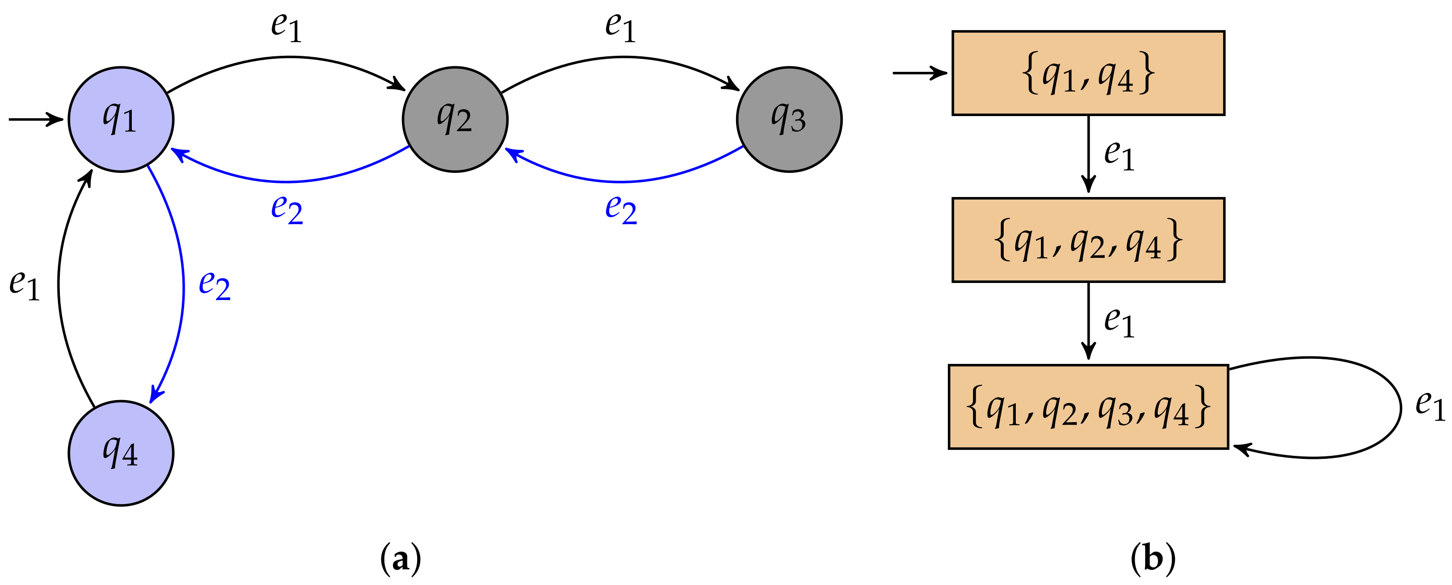
Figure 1.
(a) A system and (b) the observer with respect to .

Figure 2.
The generation of observations.

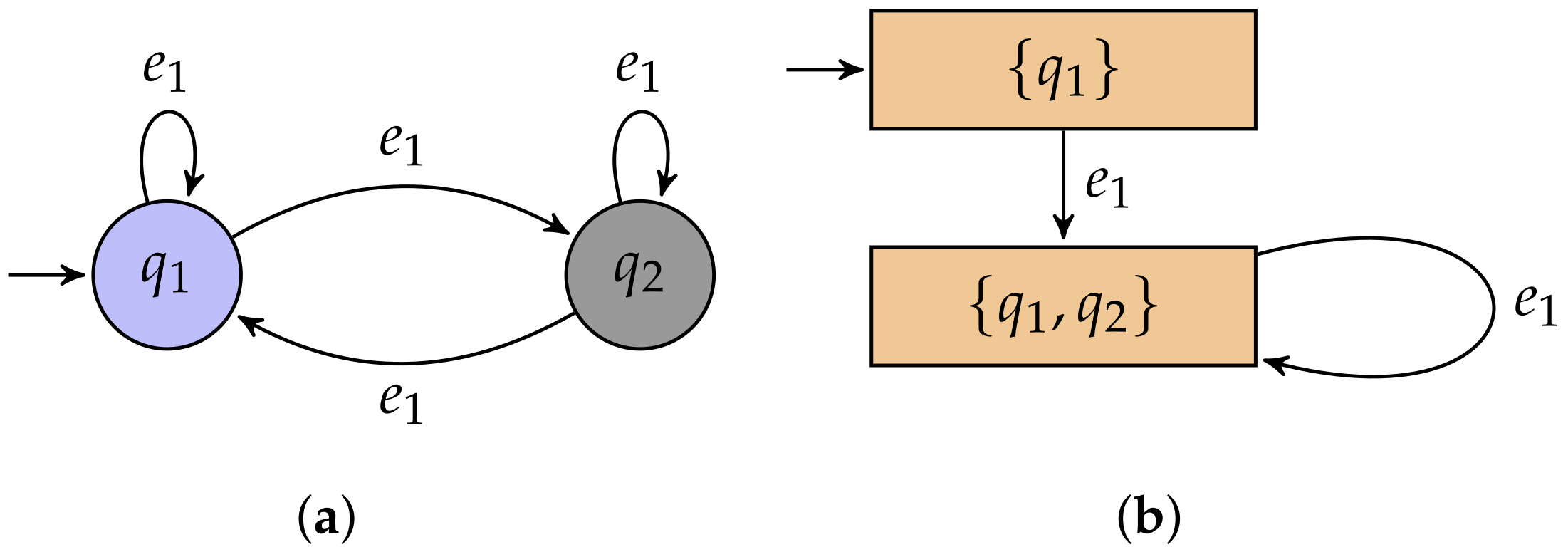
Figure 3.
(a) A system and (b) the observer with respect to .

Figure 4.
Input and output of Algorithm 2.

Figure 5.
(a) A single-story building with five rooms and (b) the constructed automaton model .

Figure 6.
The run status recorder of .


Table 1.
Number of runs in .
| Observation () | ||
|---|---|---|
| 1 | 0 | |
Disclaimer/Publisher’s Note: The statements, opinions and data contained in all publications are solely those of the individual author(s) and contributor(s) and not of MDPI and/or the editor(s). MDPI and/or the editor(s) disclaim responsibility for any injury to people or property resulting from any ideas, methods, instructions or products referred to in the content. |
© 2023 by the authors. Licensee MDPI, Basel, Switzerland. This article is an open access article distributed under the terms and conditions of the Creative Commons Attribution (CC BY) license (https://creativecommons.org/licenses/by/4.0/).
Share and Cite
MDPI and ACS Style
Zhou, S.; Yu, J.; Yin, L.; Li, Z. Security Quantification for Discrete Event Systems Based on the Worth of States. Mathematics 2023, 11, 3629. https://0-doi-org.brum.beds.ac.uk/10.3390/math11173629
AMA Style
Zhou S, Yu J, Yin L, Li Z. Security Quantification for Discrete Event Systems Based on the Worth of States. Mathematics. 2023; 11(17):3629. https://0-doi-org.brum.beds.ac.uk/10.3390/math11173629
Chicago/Turabian StyleZhou, Sian, Jiaxin Yu, Li Yin, and Zhiwu Li. 2023. "Security Quantification for Discrete Event Systems Based on the Worth of States" Mathematics 11, no. 17: 3629. https://0-doi-org.brum.beds.ac.uk/10.3390/math11173629
Note that from the first issue of 2016, this journal uses article numbers instead of page numbers. See further details here.