One Approach to Numerical Modeling of the Heat and Mass Transfers of Two-Phase Fluids in Fractured-Porous Reservoirs

Abstract

The work is devoted to numerical modeling of the processes of heat and mass transfer of a two-phase fluid in the environment of a production well, which is necessary for monitoring the development of fractured-porous reservoirs. This work proposes an efficient approach to constructing a solution to the problem. To solve the problem, a model of the “double medium” type is used, where the pore part of the reservoir is considered as the first medium, and the system of natural fractures is considered as the second medium. For the resulting mathematical model, the difference schemes with time weights are constructed based on the algorithm of splitting by physical processes, which ensure the correctness and consistency of fluxes in the fracture system and the pore reservoir. In the numerical solution, the approximations of differential operators obtained in the framework of the finite difference method are used. For the parallel implementation of the developed numerical approach, the domain decomposition method and the matrix sweep algorithm are chosen. The program implementation is made using the MPI standard. Computational experiments are carried out, the results of which confirm the effectiveness of the developed numerical algorithm and its parallel implementation. In numerical experiments, the distributions of pressure and temperature near an operating production well are obtained, on the basis of which it is possible to adjust the operation of wells in order to increase production.

1. Introduction

Many processes of heat and mass transfer occurring in nature are accompanied by the transfer of the mass of one substance to the mass of another substance [1,2]. These processes are of great practical importance in various fields. One of these areas is the oil and gas industry, where the use of scientific approaches to improve development technologies is an integral part.

To date, the scale of hydrocarbon production has significantly increased, new fields with complex geological conditions are being put into development. And each new open object most often has degraded filtration properties, which requires new approaches to development. In this regard, the level of requirements for the study of the movement of liquids (gas, oil and water) in operated reservoirs has significantly increased.

Oil fields are confined to uplifts of sedimentary rocks, which are accumulations of grains of minerals interconnected as a result of geological processes [3]. In carbonate rocks, the pore system is characterized by strong heterogeneity, while the system of secondary voids is more developed. Secondary voids include fractures caused by tectonic stresses and caverns resulting from various chemical reactions [4,5]. The length and dimensions of fractures and cavities may exceed the dimensions of primary pores. All of the above gives the features of the well-known theory of fluid filtration in reservoirs. One of them is the need to simultaneously consider processes in different media, namely, in two different systems (a system of natural fractures and a pore part of a reservoir (matrix)) with different reservoir properties, which numerically can reach a difference of several orders of magnitude [6,7].

Information about the reservoir consists of data from the study of rock samples, hydrodynamic studies of wells, analysis of the results of oil and formation water samples, and the history of field development [1]. But with such a variety of data, the information obtained is limited and not always sufficient for unambiguously building a reservoir model. At the same time, conducted experiments at wells incur large economic costs, as well as large production losses due to shutdowns of wells for research. Under such conditions, the task of the study is to establish qualitative patterns, quantitative relationships that are resistant to variation in the initial data and expand the totality of information that cannot be obtained experimentally [8]. Therefore, the solution of practical problems of the modern oil and gas industry is possible only with the help of numerical modeling, which requires the use of the most modern developments and fast solutions.

The process considered in this work is based on the well-known equations of hydrodynamics [2,9]. For traditional filtration models of the “single medium” type, effective algorithms have been developed, both direct ones for modeling the filtration process, and methods for interpreting hydrodynamic research data to identify model parameters. However, the situation is significantly more complicated when using models related to the “dual medium” [10,11], which is associated with practical features (the presence of two systems—the pore part of the reservoir and fractures) of the process under consideration, which complicate the model.

The programs for analysis and interpretation of results that exist both in Russia and abroad do not allow for a full range of calculations and are not always computationally efficient, which limits the range of technical and economic development problems solved with their help. Therefore, there is a need to create a fast calculation tool based on effective numerical algorithms that will allow solving operational planning problems that arise during field development, which include an express assessment of the required shutdown duration before the study, as well as a thorough study of the behavior of fluid dynamics processes at various reservoir parameters.

The difficulty of solving the problem lies in the large number of variables that affect the ongoing processes, in the nonlinearity of the basic equations of hydrodynamics, heat and mass transfer, in the impossibility of obtaining all information about the course of the process due to the high laboriousness of experimental studies [12].

Numerical modeling of such processes is also associated with great difficulties, similarly associated with a large number of unknowns and the use of small time steps [12,13]. The possibilities of modern computer technologies make it possible to implement tasks of this kind. To successfully solve the problem, an efficient numerical algorithm is needed, with the possibility of running on the architecture of large supercomputers.

In our previous works [14,15], the isothermal process of mass transfer of a two-phase fluid in a fractured-porous reservoir was considered in a one-dimensional setting. An original implicit finite-difference scheme on a non-uniform spatial grid and a parallel algorithm for solving the problem were proposed. The obtained calculation results confirmed the efficiency of the proposed algorithm and its parallel implementation.

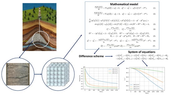
In this work, we consider a non-isothermal process of heat and mass transfer of a two-phase fluid in a carbonate reservoir of a fractured porous type. A new mathematical model has been constructed for it, which additionally includes the energy equation. For this model, an original difference scheme with splitting by physical processes has been developed. The scheme ensures the correctness and consistency of fluxes between the natural fracture system and the pore reservoir. Within the framework of the program implementation, the proposed numerical algorithm was parallelized using the MPI standard and the domain decomposition technique. With the help of the developed program, a series of computational experiments was carried out. A feature of the performed calculations is the use of field and geophysical data on the production characteristics and the filtration and capacitance properties of the formations. The goals of the calculations were to determine: (a) the optimal number of processes for solving the system of difference equations; and (b) the pressure and temperature dynamics depending on formation permeability values. The results of numerical experiments confirmed the correctness and efficiency of the developed numerical approach.

2. Problem Statement

The process of heat and mass transfer of a two-phase fluid in a carbonate reservoir (see Figure 1) is considered, where there are two pore systems—a system of fractures and the pore part of the reservoir (matrices). Figure 1 presents a fragment of the reservoir. Each of the systems is characterized by its own reservoir parameters $(k,\varphi )$, the difference between which is achieved from one to several orders.

At the initial moment of time, the formation is not disturbed, i.e., initial formation pressures $\left(P_0\right)$ and temperature $\left(T_0\right)$ are set. The well is put into operation with constant bottom hole pressure $\left(Pwf\right)$. At the moment of putting into operation, due to the created depression, the inflow of fluid from the formation to the well begins. The fluid flow occurs only along the fractures, and the pore part of the reservoir (matrix) is a certain capacity of fluid accumulation and is taken into account by introducing special functions [16]. When the pressure in the fracture system decreases lower than in the pore part (matrix), fluid flows from the matrix into the fractures.

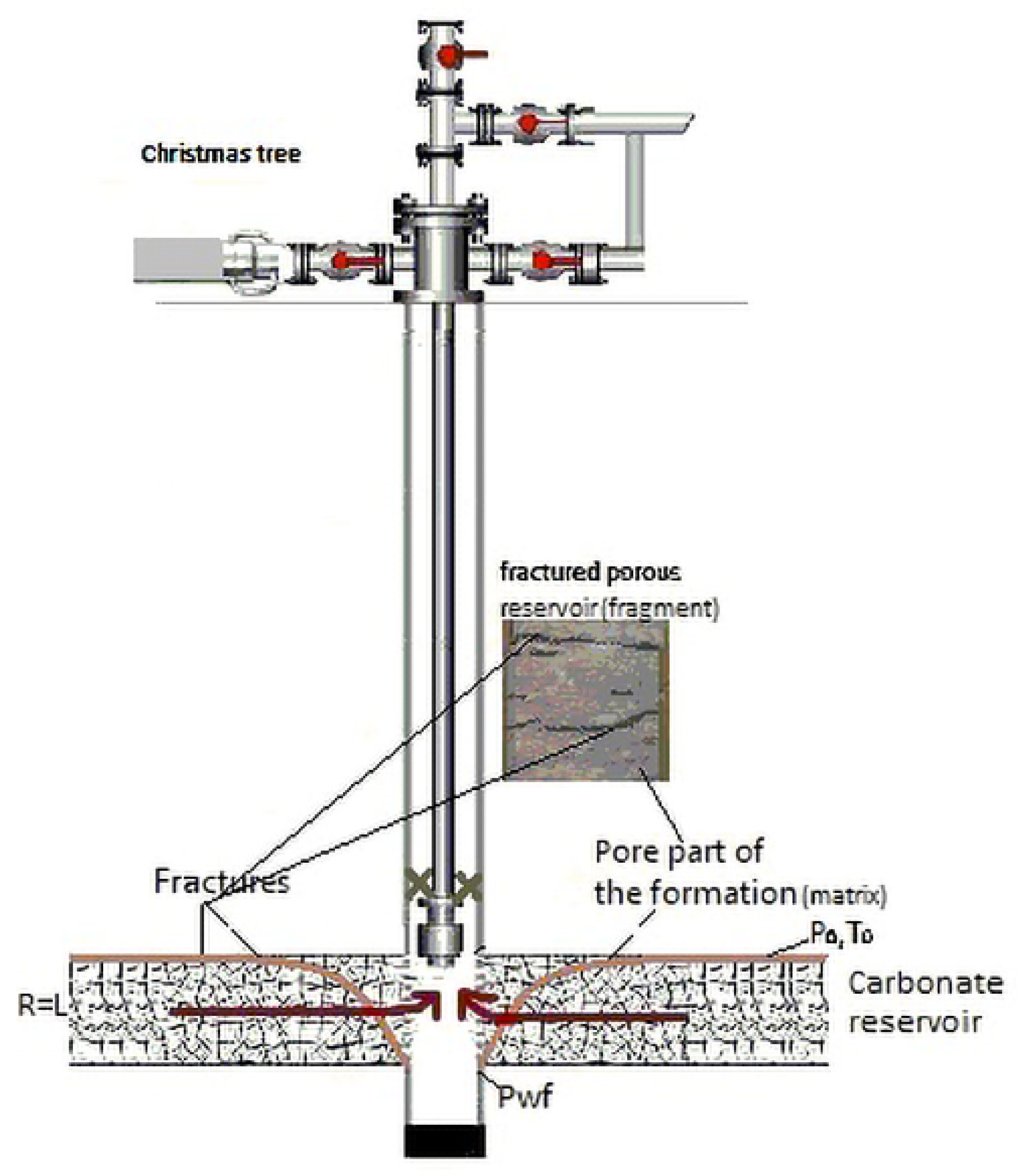
It is assumed that the reservoir is homogeneous and isotropic. The flow of a weakly compressible fluid in a system of fractures is within the validity of Darcy’s law. It is necessary to reproduce the dynamics of pressure and temperature during the operation of the well at different times and distances from the well at different values of fracture and matrix permeability. Figure 1 shows a scheme of a well and a reservoir.

The Christmas tree in Figure 1 is the system of mechanisms and devices designed to seal the mouth of pumping and fountain wells and their mutual isolation; fractures are the secondary voids caused by tectonic stresses, through which fluid flows; the pore part of the formation (matrices) is the rock that has physical properties that allow it to accumulate water, oil and gas, as well as filter and release them in the presence of a pressure drop; the carbonate reservoir is the type of reservoir, which mainly consists of limestone and dolomite, with a developed system of secondary voids; $R=L$ is the distance to which reservoir disturbances reach during well operation; $P_w^f$ is the bottom hole pressure; and $P_0$ and $T_0$ are the initial reservoir pressure and temperature.

The mathematical description of the filtration processes is presented on the basis of the classical laws of continuum mechanics [1,2].

$$\frac{\partial \left({\varphi }^{\alpha }{\rho }_o^{\alpha }{S}_o^{\alpha }\right)}{\partial t}+\nabla \left({\rho }_o^{\alpha }{\overrightarrow{U}}_o^{\alpha }\right)+q_o^{\alpha }=0,q_o^m=-q_o^f=-{\rho }_o^m\sigma {\lambda }_o^m(P^f-P^m),$$

(1)

$$\frac{\partial \left({\varphi }^{\alpha }{\rho }_w^{\alpha }{S}_w^{\alpha }\right)}{\partial t}+\nabla \left({\rho }_w^{\alpha }{\overrightarrow{U}}_w^{\alpha }\right)-q_w^{\alpha }=0,q_w^m=-q_w^f=-{\rho }_w^m\sigma {\lambda }_w^m(P^f-P^m),$$

(2)

$$\begin{array}{c}\hfill \frac{\partial }{\partial t}[({\varphi }^f{\rho }_o^f{S}_o^f{\epsilon }_o^f+{\varphi }^m{\rho }_o^m{S}_o^m{\epsilon }_o^m+{\varphi }^f{\rho }_w^f{S}_w^f{\epsilon }_w^f+{\varphi }^m{\rho }_w^m{S}_w^m{\epsilon }_w^m)+(1-{\varphi }^f-{\varphi }^m){\rho }_s{\epsilon }_s]+\\ \hfill div\left[{\rho }_o^f{\epsilon }_o^f{\overrightarrow{U}}_o^f+{\rho }_w^f{\epsilon }_w^f{\overrightarrow{U}}_w^f\right]+div\left[P^f({\overrightarrow{U}}_o^f+{\overrightarrow{U}}_w^f)\right]+div[{\overrightarrow{W}}^f+{\overrightarrow{W}}^m+{\overrightarrow{W}}_s]=0,\end{array}$$

(3)

$${\lambda }_o^m=\frac{k^m{k}_{ro}\left(S_o^m\right)}{{\mu }_o},{\lambda }_w^m=\frac{k^m{k}_{rw}\left(S_w^m\right)}{{\mu }_w}.$$

(4)

Here, $\alpha =f,m$, where f is the fracture system, m is the matrix system, $i=o,w$, where o is the oil, w is the water, $P^f$ is the formation pressure in the fracture system (Pa), $P^m$ is the formation pressure in the matrix (Pa), ${\varphi }^f$ is the porosity in the fracture system, ${\varphi }^m$ is the porosity in the matrix, ${\rho }_o^{\alpha }$ is the density of oil $(g/m^3)$, ${\rho }_w^{\alpha }$ is the density of water $(g/m^3)$, $S_i^f$ is the saturation of oil or water in the fracture system, $S_i^m$ is the saturation of oil or water in the matrix, ${\overrightarrow{U}}_i^{\alpha }$ is the flow velocity of oil or water, $q_i^{\alpha }$ is the function of redistribution of the fluid between the matrix and the fractures, $\sigma$ is the coefficient of fractured rock $(1/m^2)$, ${\epsilon }_i^{\alpha }$ is the energy of oil/water, s is rock skeleton, ${\rho }_s,{\epsilon }_s$ is the density and energy of the system, $k^{\alpha }$ is the absolute permeability $\left(m^2\right)$, $k_{rw}$ and $k_{ro}$ are the relative phase permeabilities of water and oil, ${\mu }_o$ is the viscosity of oil (Pa·s), and ${\mu }_w$ is the viscosity of water (Pa·s).

Let us introduce notations:

$$\begin{array}{c}\hfill {\overrightarrow{W}}^f=-\left({\varphi }^f[S_w^f{\eta }_w^f+(1-S_w^f){\eta }_o^f]\right)\nabla T,{\overrightarrow{W}}^m=-\left({\varphi }^m[S_w^m{\eta }_w^m+(1-S_w^m){\eta }_o^m]\right)\nabla T,\\ \hfill {\overrightarrow{W}}_s=-[1-{\varphi }^f-{\varphi }^m]{\eta }_s\nabla T,\overrightarrow{W}={\overrightarrow{W}}^f+{\overrightarrow{W}}^m+{\overrightarrow{W}}_s,\end{array}$$

(5)

where T is the temperature (K), and ${\eta }_w^f,{\eta }_w^m,{\eta }_s$ are the thermal conductivity coefficients in the system of fracture, matrix and skeleton.

The flow of fluid from the pore part of the reservoir into fractures is described by the following functions:

$$\begin{array}{c}\hfill q_o^m=-q_o^f=-\frac{\sigma {\rho }_o^m{k}^m{k}_{ro}\left(S_o^m\right)}{{\mu }_o}(P^f-P^m),q_w^m=-q_w^f=-\frac{\sigma {\rho }_w^m{k}^m{k}_{rw}\left(S_w^m\right)}{{\mu }_w}(P^f-P^m).\end{array}$$

(6)

The generalized Darcy’s law is applied, according to which the filtration velocities of oil and water are equal to:

$${\overrightarrow{U}}_o^{\alpha }=-\frac{k^{\alpha }{k}_{ro}\left(S_o^{\alpha }\right)}{{\mu }_o}grad{P}^{\alpha },{\overrightarrow{U}}_w^{\alpha }=-\frac{k^{\alpha }{k}_{rw}\left(S_w^{\alpha }\right)}{{\mu }_w}grad{P}^{\alpha }.$$

(7)

Here, $\alpha =f,{\overrightarrow{U}}_o^m={\overrightarrow{U}}_w^m=0$.

We note that the investigated well is not affected by wells of the environment, while the reservoir is presented as infinite. In this regard, the right boundary condition is represented by constant pressure and temperature at the boundary, the left boundary condition is set by constant bottom hole pressure and temperature. For the initial condition, reservoir pressures and temperatures in the matrix and fractures at the initial time are used.

Problems (1)–(7) are a complex system of equations of mathematical physics of a mixed type. An important circumstance is that the problem formulated in the form of conservation laws, with a common matrix of the system with respect to water saturation, pressure and temperature, has mixed hyperbolic and parabolic properties. The direct use of such a system for the purposes of determining the dynamics of the above variables and constructing an implicit difference scheme required for calculating parabolic equations with large time steps is difficult. Accordingly, the numerical solution is not a trivial problem. To solve this problem for the initial equations, the method of splitting by physical processes [9,12,17,18] is used, where the equations are separated into the piezoconductive part and with respect to saturation transfer.

System (1)–(7), after some algebraic transformations, will be presented in the following form:

$$\begin{array}{c}\hfill \frac{S_w^f}{{\rho }_w^f}{\left[{\varphi }^f{\rho }_w^f\right]}_t+\frac{(1-S_w^f)}{{\rho }_o^f}{\left[{\varphi }^f{\rho }_o^f\right]}_t+DI{G}^f=0,\\ \hfill DI{G}^f=\frac{1}{{\rho }_w^f}div\left({\rho }_w^f{\overrightarrow{U}}_w^f\right)+\frac{1}{{\rho }_o^f}div\left({\rho }_w^f{\overrightarrow{U}}_o^f\right)+\frac{q_w^f}{{\rho }_w^f}+\frac{q_o^f}{{\rho }_o^f},\end{array}$$

(8)

$$\begin{array}{c}\hfill \frac{S_w^m}{{\rho }_w^m}{\left[{\varphi }^m{\rho }_w^m\right]}_t+\frac{(1-S_w^m)}{{\rho }_o^m}{\left[{\varphi }^m{\rho }_o^m\right]}_t+DI{G}^m=0,DI{G}^m=\frac{q_w^m}{{\rho }_w^m}+\frac{q_o^m}{{\rho }_o^m},\end{array}$$

(9)

$$\begin{array}{c}\hfill {\varphi }^f\left(S_w^f{\rho }_w^f\frac{\partial {\epsilon }_w^f}{\partial t}+(1-S_w^f){\rho }_o^f\frac{\partial {\epsilon }_o^f}{\partial t}\right)+{\varphi }^m\left(S_w^m{\rho }_w^m\frac{\partial {\epsilon }_w^m}{\partial t}+(1-S_w^m){\rho }_o^m\frac{\partial {\epsilon }_o^m}{\partial t}\right)+\\ \hfill \frac{\partial }{\partial t}(1-{\varphi }^f-{\varphi }^m){\rho }_s{\epsilon }_s+DI{G}_{\epsilon }^f+DI{G}_{\epsilon }^m+div{\overrightarrow{W}}_s=0,\\ \hfill DI{G}_{\epsilon }^f=\left[div\left({\rho }_w^f{\epsilon }_w^f{\overrightarrow{U}}_w^f\right)-{\epsilon }_w^{f}div\left({\rho }_w^f{\overrightarrow{U}}_w^f\right)\right]+\left[div\left({\rho }_o^f{\epsilon }_o^f{\overrightarrow{U}}_o^f\right)-{\epsilon }_o^{f}div\left({\rho }_o^f{\overrightarrow{U}}_o^f\right)\right]+\\ \hfill +div\left[P^f({\overrightarrow{U}}_w^f+{\overrightarrow{U}}_o^f)\right]+div{\overrightarrow{W}}^f+(-{\epsilon }_w^f{q}_w^f-{\epsilon }_o^f{q}_o^f)=0,\\ \hfill DI{G}_{\epsilon }^m=div{\overrightarrow{W}}^m+(-{\epsilon }_w^m{q}_w^m-{\epsilon }_o^m{q}_o^m),\\ \hfill div{\overrightarrow{W}}^f=-\left({\varphi }^f[S_w^f{\eta }_w^f+(1-S_w^f){\eta }_o^f]\right),div{\overrightarrow{W}}^m=-\left({\varphi }^m[S_w^m{\eta }_w^m+(1-S_w^m){\eta }_o^m]\right).\end{array}$$

(10)

3. Difference Scheme Construction

A one-dimensional statement of Problems (1)–(7) is considered. An implicit finite-difference scheme on a uniform grid is used to solve partial differential equations [15,19,20]. Note that the approach presented below will be the basis for the problem in the multidimensional case. The use of a non-uniform grid is also possible for this statement.

$${\overline{W}}_h=(x_i=ih,i=0,1,\dots ,N,x_0=0,x_N=L),{\overline{W}}_{\tau }=(t_j=k\tau ,k=0,1,\dots ,M),$$

(11)

where $x_i$ are the coordinates of grid nodes in space, h is the grid step in radius, $t_j$ are the coordinates of grid nodes in time, $\tau$ is the grid step in time, and N and M are the number of nodes in space and time, respectively. The grid values (pressure and saturation) are determined in $x_i$. The $i+1/2$-th cell of a one-dimensional grid ${\Omega }_i$ is understood as a segment $[x_i,x_{i+1}]$. $h_{i+\frac{1}{2}}=x_{i+1}-x_i$, ${\hslash }_i=(h_{i+\frac{1}{2}}+h_{i-\frac{1}{2}})/2.$

Differential Equations (1)–(3) are approximated by their grid analogues [19,20]:

$${\left({\overline{\varphi }}^{\alpha }{\rho }_o^{\alpha }{S}_o^{\alpha }\right)}_t+DIN{\left({\rho }_o^{\alpha }{U}_o^{\alpha }\right)}^{\sim }+q_o^{\alpha \sim }=0,q_o^{m\sim }=-q_o^{f\sim }=-{\rho }_o^{m\sim }{\overline{\sigma }}^{\sim }{\lambda }_o^{m\sim }(P^{f\sim }-P^{m\sim }),$$

(12)

$${\left({\overline{\varphi }}^{\alpha }{\rho }_w^{\alpha }{S}_w^{\alpha }\right)}_t+DIN{\left({\rho }_w^{\alpha }{U}_w^{\alpha }\right)}^{\sim }+q_w^{\alpha \sim }=0,q_w^{m\sim }=-q_w^{f\sim }=-{\rho }_w^{m\sim }{\overline{\sigma }}^{\sim }{\lambda }_w^{m\sim }(P^{f\sim }-P^{m\sim }),$$

(13)

$$\begin{array}{c}\hfill {[({\overline{\varphi }}^f{\rho }_o^f{S}_o^f{\epsilon }_o^f+{\overline{\varphi }}^m{\rho }_o^m{S}_o^m{\epsilon }_o^m+{\overline{\varphi }}^f{\rho }_w^f{S}_w^f{\epsilon }_w^f+{\overline{\varphi }}^m{\rho }_w^m{S}_w^m{\epsilon }_w^m)+\overline{(1-{\varphi }^f-{\varphi }^m)}{\rho }_s{\epsilon }_s]}_t+\\ \hfill +DIN[{\left({\epsilon }_o^{f\left({\delta }_{1}f\right)}\right)}_{up}{\left({\rho }_o^f{U}_o^f\right)}^{\sim }+{\left({\epsilon }_w^{f\left({\delta }_{1}f\right)}\right)}_{up}{\left({\rho }_w^f{U}_w^f\right)}^{\sim }]+DIN{\left[P^f(U_o^f+U_w^f)\right]}^{\sim }+\\ \hfill +DIN[{\left(W^f\right)}^{\sim }+{\left(W^m\right)}^{\sim }+{\left(W_s\right)}^{\sim }]=0,\\ \hfill {\left(W^f\right)}_{k+\frac{1}{2}}^{\sim }=-{\left[{\varphi }^f(S_w^f{\eta }_w^f+(1-S_w^f){\eta }_o^f)\right]}_{k+\frac{1}{2}}^{\sim }\frac{({\hat{T}}_{k+1}-{\hat{T}}_k)}{h_{k+\frac{1}{2}}},\\ \hfill {\left(W^m\right)}_{k+\frac{1}{2}}^{\sim }=-{\left[{\varphi }^m(S_w^m{\eta }_w^m+(1-S_w^m){\eta }_o^m)\right]}_{k+\frac{1}{2}}^{\sim }\frac{({\hat{T}}_{k+1}-{\hat{T}}_k)}{h_{k+\frac{1}{2}}},\\ \hfill {\left(W_s\right)}_{k+\frac{1}{2}}^{\sim }=-{\left[(1-{\varphi }^f-{\varphi }^m){\eta }_s\right]}_{k+\frac{1}{2}}^{\sim }\frac{({\hat{T}}_{k+1}-{\hat{T}}_k)}{h_{k+\frac{1}{2}}}.\end{array}$$

(14)

Here, $\overline{\varphi }=\hslash \varphi ,\overline{(1-{\varphi }^f-{\varphi }^m)}=\hslash -{\overline{\varphi }}^f-{\overline{\varphi }}^m,{\overline{\sigma }}^{\sim }=\hslash {\sigma }^{\sim }$, ${\delta }_1$ is weight by time, $a^{\sim }$ denotes the approximation of the grid function a between the layers in time t and $\widehat{t}$, $\widehat{t}=t+\tau$, $\tau$ is the time step, and $up$ denotes an upstream approximation of the expression, ${\left(DINa\right)}_i=(a_{i+\frac{1}{2}}+a_{i-\frac{1}{2}})$, ${\delta }_{1f}=\frac{\sqrt{{\left({\varphi }^f\right)}^{\wedge }\phantom{(}}}{\sqrt{{\left({\varphi }^f\right)}^{\wedge }}+\sqrt{\left({\varphi }^f\right)}}$, ${\delta }_{1m}=\frac{\sqrt{{\left({\varphi }^m\right)}^{\wedge }\phantom{(}}}{\sqrt{{\left({\varphi }^m\right)}^{\wedge }}+\sqrt{\left({\varphi }^m\right)}}$.

After splitting, the system (12)–(14) has the form:

$$\begin{array}{c}\hfill \frac{F^f}{\tau }=\frac{{\left(S_w^f\right)}^{\left({\delta }_{1f}\right)}}{{\left({\rho }_w^f\right)}^{\left({\delta }_{1f}\right)}}{\left[{\overline{\varphi }}^f{\rho }_w^f\right]}_t+\frac{{(1-S_w^f)}^{\left({\delta }_{1f}\right)}}{{\left({\rho }_o^f\right)}^{\left({\delta }_{1f}\right)}}{\left[{\overline{\varphi }}^f{\rho }_o^f\right]}_t+{DIG}^{f\sim }=0,\\ \hfill {DIG}^{f\sim }=\frac{1}{{\left({\rho }_w^f\right)}^{\left({\delta }_{1f}\right)}}DIN{\left({\rho }_w^f{U}_w^f\right)}^{\sim }+\frac{1}{{\left({\rho }_o^f\right)}^{\left({\delta }_{1f}\right)}}DIN{\left({\rho }_o^f{U}_o^f\right)}^{\sim }+\frac{q_o^{f\sim }}{{\left({\rho }_o^f\right)}^{\left({\delta }_{1f}\right)}}+\frac{q_w^{f\sim }}{{\left({\rho }_w^f\right)}^{\left({\delta }_{1f}\right)}},\end{array}$$

(15)

$$\begin{array}{c}\hfill \frac{F^m}{\tau }=\frac{{\left(S_w^m\right)}^{\left({\delta }_{1m}\right)}}{{\left({\rho }_w^m\right)}^{\left({\delta }_{1m}\right)}}{\left[{\overline{\varphi }}^m{\rho }_w^m\right]}_t+\frac{{(1-S_w^m)}^{\left({\delta }_{1m}\right)}}{{\left({\rho }_o^m\right)}^{\left({\delta }_{1m}\right)}}{\left[{\overline{\varphi }}^m{\rho }_o^m\right]}_t+{DIG}^{m\sim }=0,\\ \hfill {DIG}^{m\sim }=\frac{q_o^{m\sim }}{{\left({\rho }_o^m\right)}^{\left({\delta }_{1m}\right)}}+\frac{q_w^{m\sim }}{{\left({\rho }_w^m\right)}^{\left({\delta }_{1m}\right)}},\end{array}$$

(16)

$$\begin{array}{c}\hfill -\frac{{\Phi }_{\epsilon k}}{\tau }={\left({\overline{\varphi }}^f\right)}^{(1-{\delta }_{1f})}\left({\left[S_w^f{\rho }_w^f\right]}^{\left({\delta }_{1f}\right)}{\left({\epsilon }_w^f\right)}_t+{\left[(1-S_w^f){\rho }_o^f\right]}^{\left({\delta }_{1f}\right)}{\left({\epsilon }_o^f\right)}_t\right)+\\ \hfill +{\left({\overline{\varphi }}^m\right)}^{(1-{\delta }_{1m})}\left({\left[S_w^m{\rho }_w^m\right]}^{\left({\delta }_{1m}\right)}{\left({\epsilon }_w^m\right)}_t+{\left[(1-S_w^m){\rho }_o^m\right]}^{\left({\delta }_{1m}\right)}{\left({\epsilon }_o^m\right)}_t\right)+{\left(\overline{(1-{\varphi }^f-{\varphi }^m)}{\rho }_s{\epsilon }_s)\right)}_t+\\ \hfill +{DIG}_{\epsilon }^{f\sim }+{DIG}_{\epsilon }^{m\sim }+{DINW}_s^{\sim }=0,\\ \hfill {DIG}_{\epsilon }^{f\sim }=\left(DIN\left[{\left({\epsilon }_w^{f\left({\delta }_{1f}\right)}\right)}_{up}{\left({\rho }_w^f{U}_w^f\right)}^{\sim }\right]-{\epsilon }_w^{f\left({\delta }_{1f}\right)}DIN{\left({\rho }_w^f{U}_w^f\right)}^{\sim }\right)+\\ \hfill +\left(DIN\left[{\left({\epsilon }_o^{f\left({\delta }_{1f}\right)}\right)}_{up}{\left({\rho }_o^f{U}_o^f\right)}^{\sim }\right]-{\epsilon }_o^{f\left({\delta }_{1f}\right)}DIN{\left({\rho }_o^f{U}_o^f\right)}^{\sim }\right)+\\ \hfill +DIN{\left[P^f\left(U_w^f+U_o^f\right)\right]}^{\sim }+{DINW}^{f\sim }-{\left({\epsilon }_w^f\right)}^{\left({\delta }_{1f}\right)}{q}_w^{f\sim }-{\left({\epsilon }_o^f\right)}^{\left({\delta }_{1f}\right)}{q}_o^{f\sim },\\ \hfill {DIG}_{\epsilon }^{m\sim }={DINW}^{m\sim }-{\left({\epsilon }_w^m\right)}^{\left({\delta }_{1m}\right)}{q}_w^{m\sim }-{\left({\epsilon }_o^m\right)}^{\left({\delta }_{1m}\right)}{q}_o^{m\sim }.\end{array}$$

(17)

As a result of the linearization of Equation (16), we obtain a relationship between the increments of pressures in the matrix $\left(\delta P^f\right)$ and in the fracture $\left(\delta P^m\right)$, temperature $\left(\delta T\right)$ and the residual $\left({\Phi }^{ms}\right)$.

$$\delta P^m={\pi }_m^s\delta P^f-{\Phi }^{ms}-\frac{{\Theta }_{T_m}^s}{{\Theta }_{P_{m\tau }}^s}\delta T,$$

(18)

where

$${\pi }_m^s=\frac{\tau }{{\Theta }_{P_{m\tau }}^s}\left(\frac{{\left({\rho }_w^m\overline{\sigma }{\lambda }_w^m\right)}^s}{{\left({\rho }_w^m\right)}^{{\left({\delta }_{1m}\right)}^{\approx }}}+(\frac{{\left({\rho }_o^m\overline{\sigma }{\lambda }_o^m\right)}^s}{{\left({\rho }_o^m\right)}^{{\left({\delta }_{1m}\right)}^{\approx }}}\right),{\Phi }^{ms}=\frac{F^{ms}}{{\Theta }_{P_{m\tau }}^s},$$

(19)

$$\begin{array}{c}\hfill {\Theta }_{P_{m\tau }}^s={\Theta }_{P_m}^s+\tau \left(\frac{{\left({\rho }_w^m\overline{\sigma }{\lambda }_w^m\right)}^s}{{\left({\rho }_w^m\right)}^{{\left({\delta }_{1m}\right)}^{\approx }}}+(\frac{{\left({\rho }_o^m\overline{\sigma }{\lambda }_o^m\right)}^s}{{\left({\rho }_o^m\right)}^{{\left({\delta }_{1m}\right)}^{\approx }}}\right),\\ \hfill {\Theta }_{P_m}^s=\frac{{\left(S_w^m\right)}^{\left({\delta }_{1m}\right)\approx }}{{\left({\rho }_w^m\right)}^{\left({\delta }_{1m}\right)\approx }}{\left({\overline{\varphi }}^m{\rho }_w^m\right)}_{P_m}^{\prime s}+\frac{{\left(1-S_w^m\right)}^{\left({\delta }_{1m}\right)\approx }}{{\left({\rho }_o^m\right)}^{\left({\delta }_{1m}\right)\approx }}{\left({\overline{\varphi }}^m{\rho }_o^m\right)}_{P_m}^{\prime s},\end{array}$$

(20)

$${\Theta }_{T_m}^s=\frac{{\left(S_w^m\right)}^{\left({\delta }_{1m}\right)\approx }}{{\left({\rho }_w^m\right)}^{\left({\delta }_{1m}\right)\approx }}{\left({\overline{\varphi }}^m{\rho }_w^m\right)}_T^{\prime s}+\frac{{\left(1-S_w^m\right)}^{\left({\delta }_{1m}\right)\approx }}{{\left({\rho }_o^m\right)}^{\left({\delta }_{1m}\right)\approx }}{\left({\overline{\varphi }}^m{\rho }_o^m\right)}_T^{\prime s}.$$

(21)

Here, $a^{\approx }$ means that the meanings of the value of the implicit layer in time are taken at a known iteration. The index s, denoting a known computed iteration, has the same sense. The prime denotes the derivative with respect to thermodynamic variables (pressure or temperature). Here, $F^{ms}$ is taken from (17) with the meanings of the values of the implicit layer in time from the s–th iteration. Further, the linearized system of Equations (15) and (17), taking into account Equation (18), will have the form:

$$\begin{array}{c}\hfill -\left(A_{pk}^{11}\delta P_{k-1}^f+A_{pk}^{12}\delta T_{k-1}\right)+\left(C_{pk}^{11}\delta P_k^f+C_{pk}^{12}\delta T_k\right)-\left(B_{pk}^{11}\delta P_{k+1}^f+B_{pk}^{12}\delta T_{k+1}\right)={\Phi }_{pk}^1,\\ \hfill -\left(A_{\epsilon k}^{21}\delta P_{k-1}^f+A_{\epsilon k}^{22}\delta T_{k-1}\right)+\left(C_{\epsilon k}^{21}\delta P_k^f+C_{\epsilon k}^{22}\delta T_k\right)-\left(B_{\epsilon k}^{21}\delta P_{k+1}^f+B_{\epsilon k}^{22}\delta T_{k+1}\right)={\Phi }_{\epsilon k}^2,\end{array}$$

(22)

where the matrices have the following form:

$$A_{pk}^{12}=0,B_{pk}^{12}=0,$$

(23)

$$\begin{array}{c}\hfill A_{pk}^{11}=\frac{\tau }{{\left[{\left({\rho }_w^f\right)}^{\left({\delta }_{1f}\right)}\right]}_k^{\approx }}\left(\frac{1}{h_{k-\frac{1}{2}}}{\left(\frac{{\rho }_w^f{k}^f}{{\mu }_w^f}\right)}_{k-\frac{1}{2}}^s{k}_{rw(k-\frac{1}{2})}^{ups}\right)+\\ \hfill +\frac{\tau }{{\left[{\left({\rho }_o^f\right)}^{\left({\delta }_{1f}\right)}\right]}_k^{\approx }}\left(\frac{1}{h_{k-\frac{1}{2}}}{\left(\frac{{\rho }_o^f{k}^f}{{\mu }_o^f}\right)}_{k-\frac{1}{2}}^s{k}_{ro(k-\frac{1}{2})}^{ups}\right),\end{array}$$

(24)

$$\begin{array}{c}\hfill B_{pk}^{11}=\frac{\tau }{{\left[{\left({\rho }_w^f\right)}^{\left({\delta }_{1f}\right)}\right]}_k^{\approx }}\left(\frac{1}{h_{k+\frac{1}{2}}}{\left(\frac{{\rho }_w^f{k}^f}{{\mu }_w^f}\right)}_{k+\frac{1}{2}}^s{k}_{rw(k+\frac{1}{2})}^{ups}\right)+\\ \hfill +\frac{\tau }{{\left[{\left({\rho }_o^f\right)}^{\left({\delta }_{1f}\right)}\right]}_k^{\approx }}\left(\frac{1}{h_{k+\frac{1}{2}}}{\left(\frac{{\rho }_o^f{k}^f}{{\mu }_o^f}\right)}_{k+\frac{1}{2}}^s{k}_{ro(k+\frac{1}{2})}^{ups}\right),\end{array}$$

(25)

$$\begin{array}{c}\hfill C_{pk}^{11}={\left[\frac{{\left(S_w^f\right)}^{\left({\delta }_{1f}\right)\approx }}{{\left({\rho }_w^f\right)}^{\left({\delta }_{1f}\right)\approx }}{\left({\overline{\varphi }}^f{\rho }_w^f\right)}_{P_f}^{\prime s}+\frac{{\left(1-S_w^f\right)}^{\left({\delta }_{1f}\right)\approx }}{{\left({\rho }_o^f\right)}^{\left({\delta }_{1f}\right)\approx }}{\left({\overline{\varphi }}^f{\rho }_o^f\right)}_{P_f}^{\prime s}\right]}_k+\\ \hfill +\frac{\tau }{{\left[{\left({\rho }_w^f\right)}^{\left({\delta }_{1f}\right)}\right]}_k^{\approx }}\left(\frac{1}{h_{k+\frac{1}{2}}}{\left(\frac{{\rho }_w^f{k}^f}{{\mu }_w^f}\right)}_{k+\frac{1}{2}}^s{k}_{rw(k+\frac{1}{2})}^{ups}+\frac{1}{h_{k-\frac{1}{2}}}{\left(\frac{{\rho }_w^f{k}^f}{{\mu }_w^f}\right)}_{k-\frac{1}{2}}^s{k}_{rw(k-\frac{1}{2})}^{ups}\right)+\\ \hfill +\frac{\tau }{{\left[{\left({\rho }_o^f\right)}^{\left({\delta }_{1f}\right)}\right]}_k^{\approx }}\left(\frac{1}{h_{k+\frac{1}{2}}}{\left(\frac{{\rho }_o^f{k}^f}{{\mu }_o^f}\right)}_{k+\frac{1}{2}}^s{k}_{ro(k+\frac{1}{2})}^{ups}+\frac{1}{h_{k-\frac{1}{2}}}{\left(\frac{{\rho }_o^f{k}^f}{{\mu }_o^f}\right)}_{k-\frac{1}{2}}^s{k}_{ro(k-\frac{1}{2})}^{ups}\right)+\\ \hfill +{\left(\frac{\tau }{{\left({\rho }_w^f\right)}^{{\left({\delta }_{1f}\right)}^{\approx }}}{\left({\rho }_w^m\overline{\sigma }{\lambda }_w^m\right)}^s(1-{\pi }_m^s)\right)}_k+{\left(\frac{\tau }{{\left({\rho }_o^f\right)}^{{\left({\delta }_{1f}\right)}^{\approx }}}{\left({\rho }_o^m\overline{\sigma }{\lambda }_o^m\right)}^s(1-{\pi }_m^s)\right)}_k,\end{array}$$

(26)

$$\begin{array}{c}\hfill C_{pk}^{12}=(\frac{{\Theta }_{T_m}^s}{{\Theta }_{P_{m\tau }}^s}\left(\frac{{\left({\rho }_w^m\overline{\sigma }{\lambda }_w^m\right)}^s}{{\left({\rho }_w^f\right)}^{{\left({\delta }_{1f}\right)}^{\approx }}}+\frac{{\left({\rho }_o^m\overline{\sigma }{\lambda }_o^m\right)}^s}{{\left({\rho }_o^f\right)}^{{\left({\delta }_{1f}\right)}^{\approx }}}\right)\tau +\\ \hfill +\left(\frac{{\left(S_w^f\right)}^{\left({\delta }_{1f}\right)\approx }}{{\left({\rho }_w^f\right)}^{\left({\delta }_{1f}\right)\approx }}{\left({\overline{\varphi }}^f{\rho }_w^f\right)}_T^{\prime s}+\frac{{\left(1-S_w^f\right)}^{\left({\delta }_{1f}\right)\approx }}{{\left({\rho }_o^f\right)}^{\left({\delta }_{1f}\right)\approx }}{\left({\overline{\varphi }}^f{\rho }_o^f\right)}_T^{\prime s}\right){)}_k,\end{array}$$

(27)

$${\Phi }_{pk}^1=-F^{fs}-\left(\frac{{\left({\rho }_w^m\overline{\sigma }{\lambda }_w^m\right)}^s}{{\left({\rho }_w^f\right)}^{{\left({\delta }_{1f}\right)}^{\approx }}}+\frac{{\left({\rho }_o^m\overline{\sigma }{\lambda }_o^m\right)}^s}{{\left({\rho }_o^f\right)}^{{\left({\delta }_{1f}\right)}^{\approx }}}\right)\tau {\Phi }^{ms}.$$

(28)

Here, $F^{fs}$ is taken from (14) with the meanings of the values of the implicit layer in time from the s–th iteration. Then, the index $k\pm 1/2$ is replaced by $k\pm 1/2$.

$$\begin{array}{c}\hfill A_{\epsilon k}^{21}=\tau \left(\frac{1}{h_{-\frac{1}{2}}}{\left(\frac{P^f{k}^f}{{\mu }_w^f}\right)}_{-\frac{1}{2}}^s{\left(k_{rw}^{up}\right)}_{-\frac{1}{2}}^s+\frac{1}{h_{-\frac{1}{2}}}{\left(\frac{P^f{k}^f}{{\mu }_o^f}\right)}_{-\frac{1}{2}}^s{\left(k_{ro}^{up}\right)}_{-\frac{1}{2}}^s\right),\end{array}$$

(29)

$$\begin{array}{c}\hfill B_{\epsilon k}^{21}=\tau \left(\frac{1}{h_{\frac{1}{2}}}{\left(\frac{P^f{k}^f}{{\mu }_w^f}\right)}_{\frac{1}{2}}^s{\left(k_{rw}^{up}\right)}_{\frac{1}{2}}^s+\frac{1}{h_{\frac{1}{2}}}{\left(\frac{P^f{k}^f}{{\mu }_o^f}\right)}_{\frac{1}{2}}^s{\left(k_{ro}^{up}\right)}_{\frac{1}{2}}^s\right),\end{array}$$

(30)

$$\begin{array}{c}\hfill C_{\epsilon k}^{21}=C_{\epsilon k}^{f21}+C_{\epsilon k}^{m21}+C_{\epsilon k}^{s21}+C_{\epsilon P_k}^{f21},\end{array}$$

(31)

where

$$\begin{array}{c}\hfill C_{\epsilon k}^{f21}={\left({\left({\overline{\varphi }}^f\right)}^{(1-{\delta }_{1f})}\left({\left[S_w^f{\rho }_w^f\right]}^{\left({\delta }_{1f}\right)}\left[-{\left(\frac{P^f}{{\rho }_w^f}\right)}_{P_f}^{\prime }\right]+{\left[(1-S_w^f){\rho }_o^f\right]}^{\left({\delta }_{1f}\right)}\left[-{\left(\frac{P^f}{{\rho }_o^f}\right)}_{P_f}^{\prime }\right]\right)\right)}^{\approx },\end{array}$$

(32)

$$\begin{array}{c}{C}_{\epsilon k}^{m21}=\left({\left({\overline{\varphi }}^m\right)}^{(1-{\delta }_{1m})}\right({\left[S_w^m{\rho }_w^m\right]}^{\left({\delta }_{1m}\right)}\left[-{\left(\frac{P^m}{{\rho }_w^m}\right)}_{P_m}^{\prime }{\pi }_m^s\right]+ \hfill \\ \hfill +{\left[(1-S_w^m){\rho }_o^m\right]}^{\left({\delta }_{1m}\right)}\left[-{\left(\frac{P^m}{{\rho }_o^m}\right)}_{P_m}^{\prime }{\pi }_m^s\right]){)}^{\approx },\end{array}$$

(33)

$$\begin{array}{c}\hfill C_{\epsilon k}^{s21}={\left({\left(\overline{(1-{\varphi }^f-{\varphi }^m)}{\rho }_s\left[-\left(\frac{P^s}{{\rho }^s}\right)\right]\right)}_{P_s}^{\prime }\left[{\left(P_s\right)}_{P_f}^{\prime }+{\left(P_s\right)}_{P_m}^{\prime }{\pi }_m^s\right]\right)}^{\approx },\end{array}$$

(34)

$$\begin{array}{c}\hfill C_{\epsilon pk}^{f21}=\tau \left(\frac{1}{h_{-\frac{1}{2}}}{\left(\frac{P^f{k}^f}{{\mu }_w^f}\right)}_{-\frac{1}{2}}^s{\left(k_{rw}^{up}\right)}_{-\frac{1}{2}}^s+\frac{1}{h_{-\frac{1}{2}}}{\left(\frac{P^f{k}^f}{{\mu }_o^f}\right)}_{-\frac{1}{2}}^s{\left(k_{ro}^{up}\right)}_{-\frac{1}{2}}^s\right)+\\ \hfill +\tau \left(\frac{1}{h_{\frac{1}{2}}}{\left(\frac{P^f{k}^f}{{\mu }_w^f}\right)}_{\frac{1}{2}}^s{\left(k_{rw}^{up}\right)}_{\frac{1}{2}}^s+\frac{1}{h_{\frac{1}{2}}}{\left(\frac{P^f{k}^f}{{\mu }_o^f}\right)}_{\frac{1}{2}}^s{\left(k_{ro}^{up}\right)}_{\frac{1}{2}}^s\right),\end{array}$$

(35)

$$\begin{array}{c}\hfill A_{\epsilon k}^{22}=\frac{\tau }{h_{-\frac{1}{2}}}{\left({\varphi }^f\left[S_w^f{\eta }_w^f+(1-S_w^f){\eta }_o^f\right]\right)}_{-\frac{1}{2}}^{\approx }+\frac{\tau }{h_{-\frac{1}{2}}}{\left({\varphi }^m\left[S_w^m{\eta }_w^m+(1-S_w^m){\eta }_o^m\right]\right)}_{-\frac{1}{2}}^{\approx }+\\ \hfill +\frac{\tau }{h_{-\frac{1}{2}}}{\left((1-{\varphi }^f-{\varphi }^m){\eta }_s\right)}_{-\frac{1}{2}}^{\approx },\end{array}$$

(36)

$$\begin{array}{c}\hfill B_{\epsilon k}^{22}=\frac{\tau }{h_{\frac{1}{2}}}{\left({\varphi }^f\left[S_w^f{\eta }_w^f+(1-S_w^f){\eta }_o^f\right]\right)}_{\frac{1}{2}}^{\approx }+\frac{\tau }{h_{\frac{1}{2}}}{\left({\varphi }^m\left[S_w^m{\eta }_w^m+(1-S_w^m){\eta }_o^m\right]\right)}_{\frac{1}{2}}^{\approx }+\\ \hfill +\frac{\tau }{h_{\frac{1}{2}}}{\left((1-{\varphi }^f-{\varphi }^m){\eta }_s\right)}_{\frac{1}{2}}^{\approx }.\end{array}$$

(37)

Here, it is supposed to be $P^s=({\varphi }^f{P}^f+{\varphi }^m{P}^m)/({\varphi }^f+{\varphi }^m)$. Next, we denote the specific heat capacity at constant pressure by $C_p$ and have the following:

$$C_{\epsilon k}^{22}=C_{\epsilon k}^{f22}+C_{\epsilon k}^{m22}+C_{\epsilon k}^{s22}+C_{\eta k}^{f22}+C_{\eta k}^{m22}+C_{\eta k}^{s22},$$

(38)

where

$$\begin{array}{c}\hfill C_{\epsilon k}^{f22}=\left({\left({\overline{\varphi }}^f\right)}^{(1-{\delta }_{1f})}\right({\left[S_w^f{\rho }_w^f\right]}^{\left({\delta }_{1f}\right)}\left[c_{\rho w}^f-{\left(\frac{P^f}{{\rho }_w^f}\right)}_T^{\prime }\right]+\\ \hfill +{\left[(1-S_w^f){\rho }_o^f\right]}^{\left({\delta }_{1f}\right)}\left[c_{\rho o}^f-{\left(\frac{P^f}{{\rho }_o^f}\right)}_T^{\prime }\right]){)}^{\approx },\end{array}$$

(39)

$$\begin{array}{c}\hfill C_{\epsilon k}^{m22}=\left({\left({\overline{\varphi }}^m\right)}^{(1-{\delta }_{1m})}\right({\left[S_w^m{\rho }_w^m\right]}^{\left({\delta }_{1m}\right)}\left[c_{\rho w}^m-{\left(\frac{P^m}{{\rho }_w^m}\right)}_{P_m}^{\prime }\frac{-{\Theta }_{T_m}^s}{{\Theta }_{P_m}^s}\right]+\\ \hfill +{\left[(1-S_w^m){\rho }_o^m\right]}^{\left({\delta }_{1m}\right)}\left[c_{\rho o}^m-{\left(\frac{P^m}{{\rho }_o^m}\right)}_{P_m}^{\prime }\frac{-{\Theta }_{T_m}^s}{{\Theta }_{P_m}^s}\right]){)}^{\approx },\end{array}$$

(40)

$$C_{\epsilon k}^{s22}={\left({\left(\overline{(1-{\varphi }^f-{\varphi }^m)}{\rho }_s\left[c_P^{s}T-\left(\frac{P^s}{{\rho }^s}\right)\right]\right)}_T^{\prime }\right)}^{\approx }.$$

(41)

Here, we accept ${\left(P^s\right)}_{P_m}^{\prime }={\varphi }^m/({\varphi }^f+{\varphi }^m)$ and, with this in mind, ${\left(P^s\right)}_T^{\prime }=[{\varphi }^m/({\varphi }^f+{\varphi }^m)][-{\Theta }_{T_m}^s/{\Theta }_{P_{m\tau }}^s]$.

$$C_{\eta k}^{f22}=\frac{\tau }{h_{\frac{1}{2}}}{\left({\varphi }^f\left[S_w^f{\eta }_w^f+(1-S_w^f){\eta }_o^f\right]\right)}_{\frac{1}{2}}^{\approx }+\frac{\tau }{h_{-\frac{1}{2}}}{\left({\varphi }^f\left[S_w^f{\eta }_w^f+(1-S_w^f){\eta }_o^f\right]\right)}_{-\frac{1}{2}}^{\approx },$$

(42)

$$C_{\eta k}^{m22}=\frac{\tau }{h_{\frac{1}{2}}}{\left({\varphi }^m\left[S_w^m{\eta }_w^m+(1-S_w^m){\eta }_o^m\right]\right)}_{\frac{1}{2}}^{\approx }+\frac{\tau }{h_{-\frac{1}{2}}}{\left({\varphi }^m\left[S_w^m{\eta }_w^m+(1-S_w^m){\eta }_o^m\right]\right)}_{-\frac{1}{2}}^{\approx },$$

(43)

$$C_{\eta k}^{s22}=\frac{\tau }{h_{\frac{1}{2}}}{\left((1-{\varphi }^f-{\varphi }^m){\eta }_s\right)}_{\frac{1}{2}}^{\approx },$$

(44)

$${\Phi }_{\epsilon k}^2={\Phi }_{\epsilon k}+{\Phi }_{\epsilon k}^{s2}+{\Phi }_{\epsilon k}^{m2}.$$

(45)

Here, ${\Phi }_{\epsilon k}$ is taken from Equation (17), with the meanings of the values of the implicit layer in time from the s–th iteration.

We take

$${\Phi }_{\epsilon k}^{s2}={\left(-\frac{{\varphi }^m}{{\varphi }^m+{\varphi }^f}\overline{(1-{\varphi }^f-{\varphi }^m)}\left[\frac{F^{ms}}{{\Theta }_{P_{m\tau }}^s}\right]\right)}^{\approx },$$

(46)

$$\begin{array}{c}\hfill {\Phi }_{\epsilon k}^{m2}=\left({\left({\overline{\varphi }}^m\right)}^{(1-{\delta }_{1m})}\right({\left[S_w^m{\rho }_w^m\right]}^{\left({\delta }_{1m}\right)}\left[-{\left(\frac{P^m}{{\rho }_w^f}\right)}_{Pm}^{\prime }\frac{F^{ms}}{{\Theta }_{Pm\tau }^s}\right]+\\ \hfill +{\left[(1-S_w^m){\rho }_o^m\right]}^{\left({\delta }_{1m}\right)}\left[-{\left(\frac{P^m}{{\rho }_w^f}\right)}_{Pm}^{\prime }\frac{F^{ms}}{{\Theta }_{Pm\tau }^s}\right]){)}^{\approx }.\end{array}$$

(47)

The resulting Equation (22) is represented by a system of linear algebraic equations, which is solved using a matrix sweep method on each time layer.

4. Matrix Sweep

The implicit in pressure and implicit in saturation (IMPIS) method [9] was used to numerically solve the system of equations of two-phase filtration in a fractured-pore type collector (8)–(10). The first block with respect to the pressure and temperature equations was solved using an implicit finite-difference scheme; after finding these parameters in the matrix and fractures, they proceeded to calculate the second block with respect to saturation.

As a result of the approximation of partial derivatives by the corresponding finite differences, we obtain a system of linear algebraic Equations (SLAE) (10) with a matrix of a block-tridiagonal structure [19]. For the convenience of solving, we write the SLAE (22) in the canonical form:

$$\begin{array}{c}\hfill -A_i{y}_{i-1}+C_i{y}_i-B_i{y}_{i+1}=F_i,1\le i\le N-1,\end{array}$$

(48)

$$\begin{array}{c}\hfill A_i=\left(\begin{array}{c}{a}_{i,0,0}{a}_{i,0,1}\\ a_{i,1,0}{a}_{i,1,1}\end{array}\right),B_i=\left(\begin{array}{c}{b}_{i,0,0}{b}_{i,0,1}\\ b_{i,1,0}{b}_{i,1,1}\end{array}\right),C_i=\left(\begin{array}{c}{c}_{i,0,0}{c}_{i,0,1}\\ c_{i,1,0}{c}_{i,1,1}\end{array}\right),F_i=\left(\begin{array}{c}{F}_{i,0}\\ F_{i,1}\end{array}\right),y_i=\left(\begin{array}{c}{y}_{i,0}\\ y_{i,1}\end{array}\right);\\ \hfill C_0{y}_0-B_0{y}_1=F_0,C_N{y}_N-A_N{y}_{N-1}=F_N.\end{array}$$

Here, $A,B,C$ are the square matrices (blocks) of dimension 2 by 2 (the first line is the piezoconductive part, the second line is the energy part, numbering from 0); y are the desired pressure $\delta P$ and temperature $\delta T$, and F are the vectors of dimension 2 × 1.

To solve System (48), we used the matrix sweep method, which is similar to the sweep method for scalar three-point equations [19]. To implement the method, operations on matrices are required: addition, multiplication and transposition, which were implemented as separate functions. The matrix sweep method itself is moved to a separate function, because during the calculation, it will be accessed on each layer in time (iteration). The solution consists of two steps, namely moving forward and moving backward:

$$\begin{array}{c}\hfill {\alpha }_0=C_0^{-1}{B}_0,{\beta }_0=C_0^{-1}{F}_0,{\alpha }_i={(C_i-A_i{\alpha }_{i-1})}^{-1}{B}_i,\end{array}$$

(49)

$$\begin{array}{c}\hfill {\beta }_i={(C_i-A_i{\alpha }_{i-1})}^{-1}(F_i+A_i{\beta }_{i-1}),i=1,2,\dots ,N;\\ \hfill y_N={\beta }_N,y_i={\alpha }_i{y}_{i+1}+{\beta }_i,i=N-1,N-2,\dots ,0;\\ \hfill {\alpha }_i=\left(\begin{array}{c}{\alpha }_{i,0,0}{\alpha }_{i,0,1}\\ {\alpha }_{i,1,0}{\alpha }_{i,1,1}\end{array}\right),{\beta }_i=\left(\begin{array}{c}{\beta }_{i,0}\\ {\beta }_{i,1}\end{array}\right).\end{array}$$

The formulated problem is very time-consuming; this is manifested in the modeling of filtration processes in long reservoirs. To do this, it is necessary to use grids with a large number of nodes, as a result of which the computation time increases significantly. To solve this problem, parallelization of the algorithm is used.

The matrix sweep parallelization algorithm is based on the well-known scalar sweep parallelization algorithm, and is implemented in program language C using the MPI standard [21]. But it is worth noting that, compared with scalar sweep, the coefficients of the equation in this case are matrices and vectors, respectively; it is necessary to allocate more memory for variables with the help of which the collective interaction of processes takes place.

To describe the parallel algorithm, we introduced a uniform partition of the set of grid node numbers $\Omega$ = 0, 1, …, N into adjacent non-intersecting subsets (m = 0, …, p − 1 is the logical number of the MPI process).

One of the stages of parallelizing the sweep is the solution of a short problem:

$$-{\tilde{A}}_i{y}_{i-1}+{\tilde{C}}_i{y}_i-{\tilde{B}}_i{y}_{i+1}={\tilde{F}}_i,i\in \tilde{\Omega },$$

(50)

where the index $i\pm 1$ is understood as the transition to the corresponding neighboring element from the set $\tilde{\Omega }=\{i_2^{\left(0\right)},i_1^{\left(1\right)},i_2^{\left(1\right)},i_1^{\left(2\right)},\dots ,i_1^{(p-2)},i_2^{(p-2)},i_1^{(p-1)}\}$. $\tilde{A},\tilde{B},\tilde{C},\tilde{F}$ are the coefficients of the equation, which are found from the coefficients of Equation (48) and the basis functions.

To solve a short problem, all MPI processes carry out a collective exchange of coefficients; the details of the algorithm are presented in [15]. This algorithm is implemented using the MPI_Allreduce function, the parameters of which are presented below.

For a scalar sweep, the call to this function has the following form:

MPI_Allreduce(dd,ee,4*ncp,MPI_DOUBLE,MPI_SUM,MPI_COMM_WORLD), where the function parameters are as follows: dd is the address of the beginning of the input buffer; ee is the address of the beginning of the receive buffer; 4*ncp is the number of elements in the input buffer; MPI_DOUBLE is the type of elements in the input buffer; MPI_SUM is the operation by which the reduction is performed; and MPI_COMM_WORLD is the communicator.

For a matrix sweep with a matrix dimension of 2 × 2, the call to this function has the following form:

MPI_Allreduce(dd,ee,14*ncp,MPI_DOUBLE,MPI_SUM,MPI_COMM_WORLD). Here, in the arrays dd and ee, there are three matrices, each with four elements, and one vector with two elements. The number of elements ($A,B,C,F$) from Equation (48) is 14.

Each internal process needs 14 × 2 (left and right borders) = 28 elements of the dd array. The zero and last processes have 14 elements, respectively, i.e., the number of elements in the send buffer changes.

The calculations were performed on the K100 hybrid supercomputer at the Center of Collective Usage of KIAM RAS [22].

To check the quality of parallelization with a change in the number of processes, a number of calculations were carried out for a small number of calculated time steps. For example, as a result of running the program on a grid with 1000 spatial steps and 70,000 time steps in serial mode, the calculation time is 25 s; in parallel mode on 16 processes, the calculation time is 2.8 s, while the parallelization efficiency is 0.558. This means that the overhead in the parallel variant is slightly less than half the estimated time. However, this is offset by an acceleration of almost nine times.

In the case of a multidimensional boundary value problem in rectangular domains, it is possible to effectively use the parallel sweep algorithm at the stages of implementation of iterative or time schemes with a factorized operator [23,24]. The examples are solving the multidimensional Poisson equation by the alternating direction method or solving the multidimensional heat equation using locally one-dimensional difference schemes.

5. Results

Based on the developed module, a series of computational calculations was carried out. We note that the input parameters are taken and varied on the basis of field studies at wells and various carbonate deposits in Russia. To verify the model, the calculated data were compared with the field data.

The following condition was considered for the formulation under consideration. The well has been idle for a long time. It is assumed that the pressure and temperature in the formation around the well have recovered to the initial values: $P_0^f=36$ MPa, $P_0^m=36$ MPa, $T_0=96$ °C. Wells in the environment are not affected. Then, the well in question is put into operation with a constant bottomhole pressure $P_{wf}^f=P_{wf}^m=28$ MPa. At the moment of start-up, a depression funnel is formed in the reservoir and fluid begins to flow into the well. It is necessary to investigate the behavior of pressure and temperature around the operating well at various permeability values. The following parameters were used in the calculation: $P_0^f=36\mathrm{MPa},$ $P_0^m=36\mathrm{MPa},$ $P_{wf}^f=28\mathrm{MPa},$ $P_{wf}^m=28\mathrm{MPa},$ ${\varphi }^f=0.01,$ ${\varphi }^m=0.1,$ ${\rho }_o=740{\mathrm{kg}/\mathrm{m}}^3,$ ${\rho }_w=1118{\mathrm{kg}/\mathrm{m}}^3,$ $S_w^f=0.4,$ $S_w^m=0.4,$ ${\mu }_w^f={\mu }_w^m=0.67\times {10}^{-3}$ Pa · s, ${\mu }_o^f={\mu }_o^m=0.86\times {10}^{-3}$ Pa · s, $\sigma =0.61/{\mathrm{m}}^2,$ $k_{rw}=0.03{\left(S_w\right)}^2+0.002\left(S_w\right)+0.0002,$ $k_{ro}=7.7{\left(S_w\right)}^4-12.07{\left(S_w\right)}^3+6.9{\left(S_w\right)}^2-1.8\left(S_w\right)+0.2,$ $k^f=1\times {10}^{-12}{\mathrm{m}}^2,$ $k^m=1\times {10}^{-15}{\mathrm{m}}^2.$

The computational domain starts at a distance of $0.1\mathrm{m}$ from the borehole axis, and ends at a distance of $1\mathrm{m}$ from this axis. The dimensions of the computational grid are determined by the constant spatial step $h=0.0009\mathrm{m}$ and the total number of steps $N=1000$, which is $0.9\mathrm{m}$. The initial time step is set equal to $\tau =0.1$, and varies depending on the number of iterations.

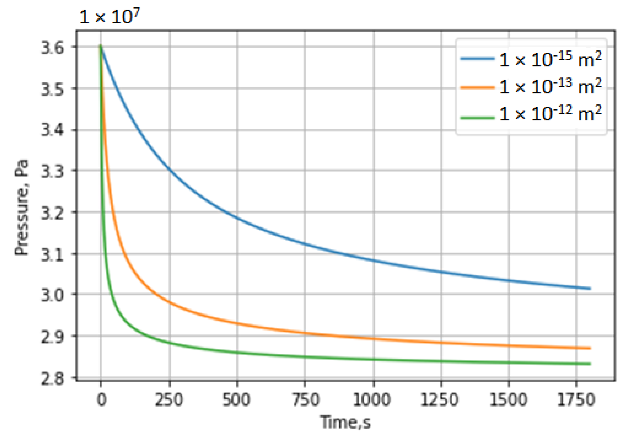
The change in permeability has the greatest effect on the pressure and temperature distribution front. Therefore, in the calculations, we will vary the values of absolute permeability in fractures. Figure 2 shows the dynamics of the pressure stabilization curves near the well for three absolute permeabilities, corresponding to $1\times {10}^{-12}{\mathrm{m}}^2,1\times {10}^{-13}{\mathrm{m}}^2,$$1\times {10}^{-15}{\mathrm{m}}^2$ We note that under given conditions with permeability, the pressure drops faster. In this regard, for reservoirs with high permeability $k^f=1\times {10}^{-12}{\mathrm{m}}^2$, it is necessary to select the characteristics of the well operation so that the pressure sinks more slowly over a short period of operation, otherwise this will lead to rapid depletion of the reservoir.

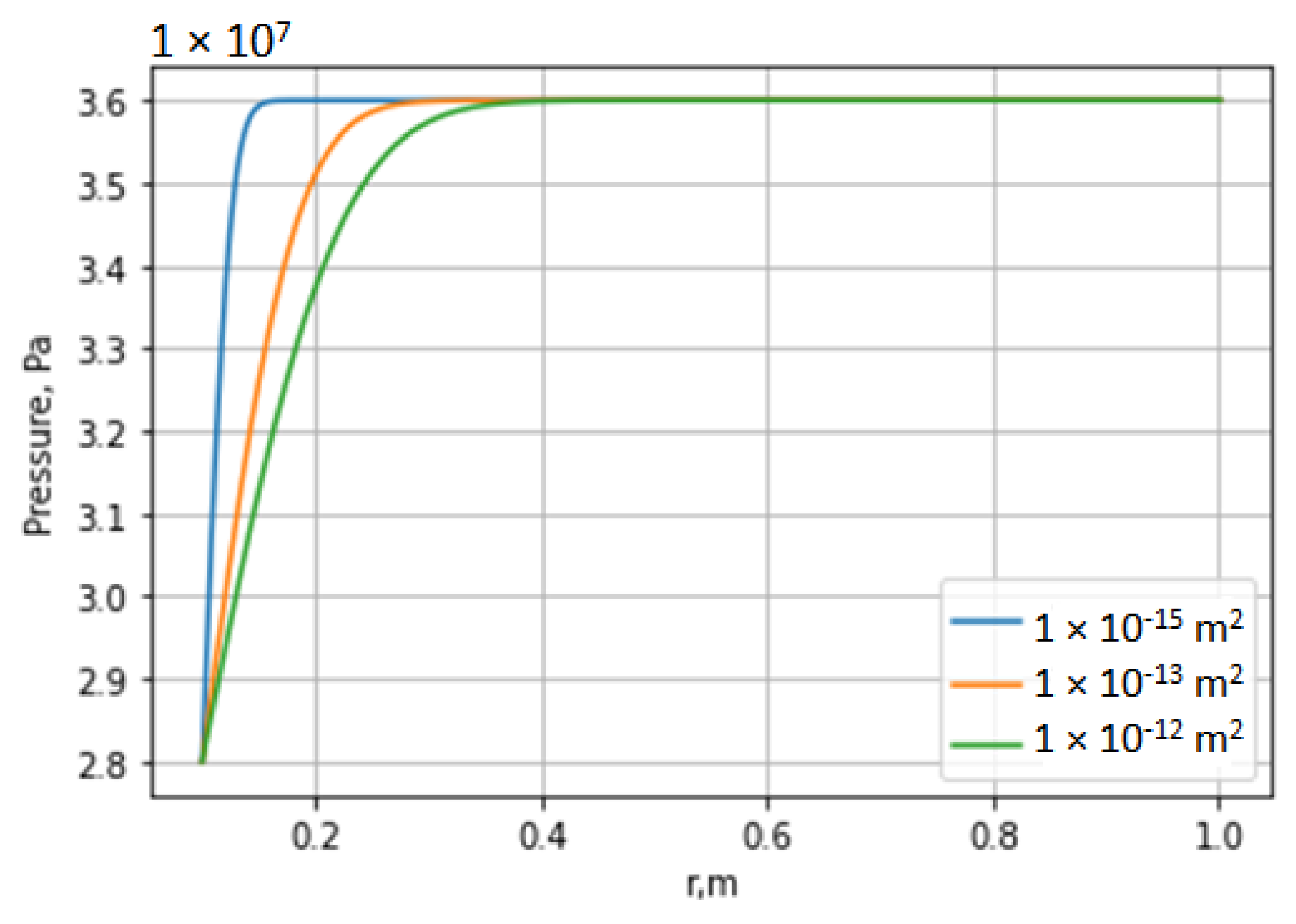
Figure 3 shows the dependence of pressure on the radius for various values of absolute permeability in fractures at the final time. Based on these calculations, it is possible to determine the area of pressure distribution for various time values. We note that at high permeability, the pressure distribution has a larger radius around the production well, which indicates a larger drainage zone.

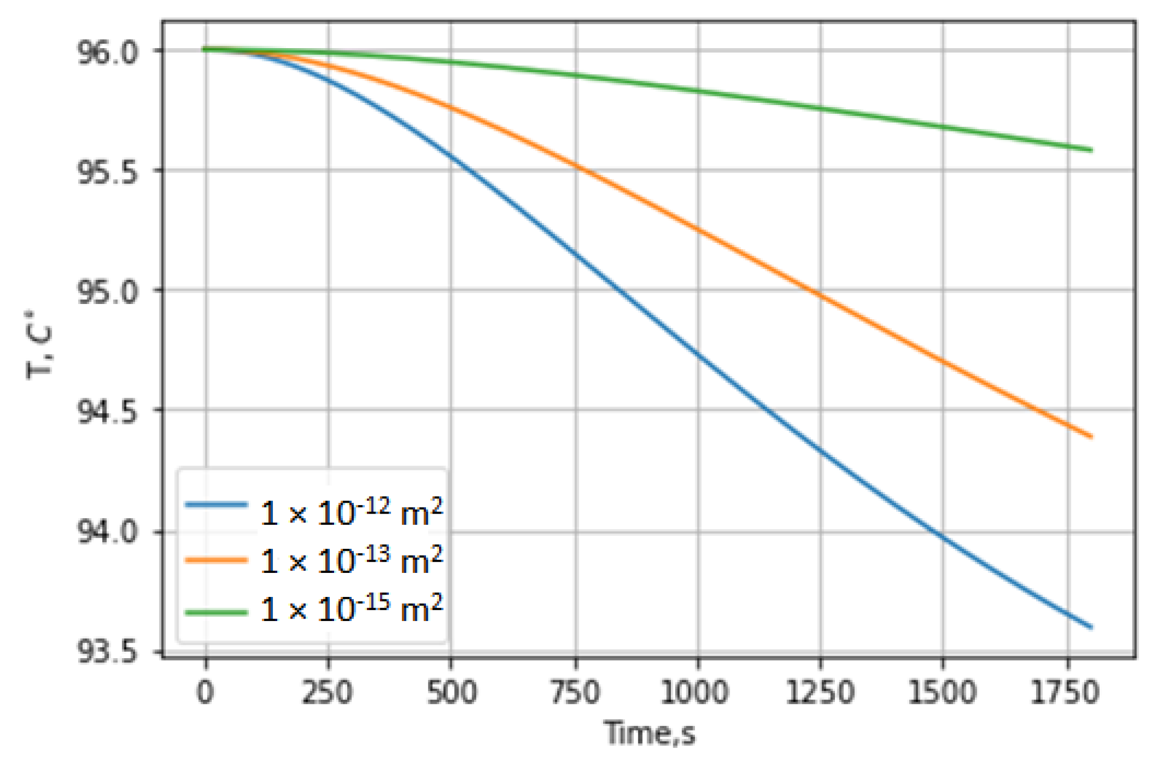
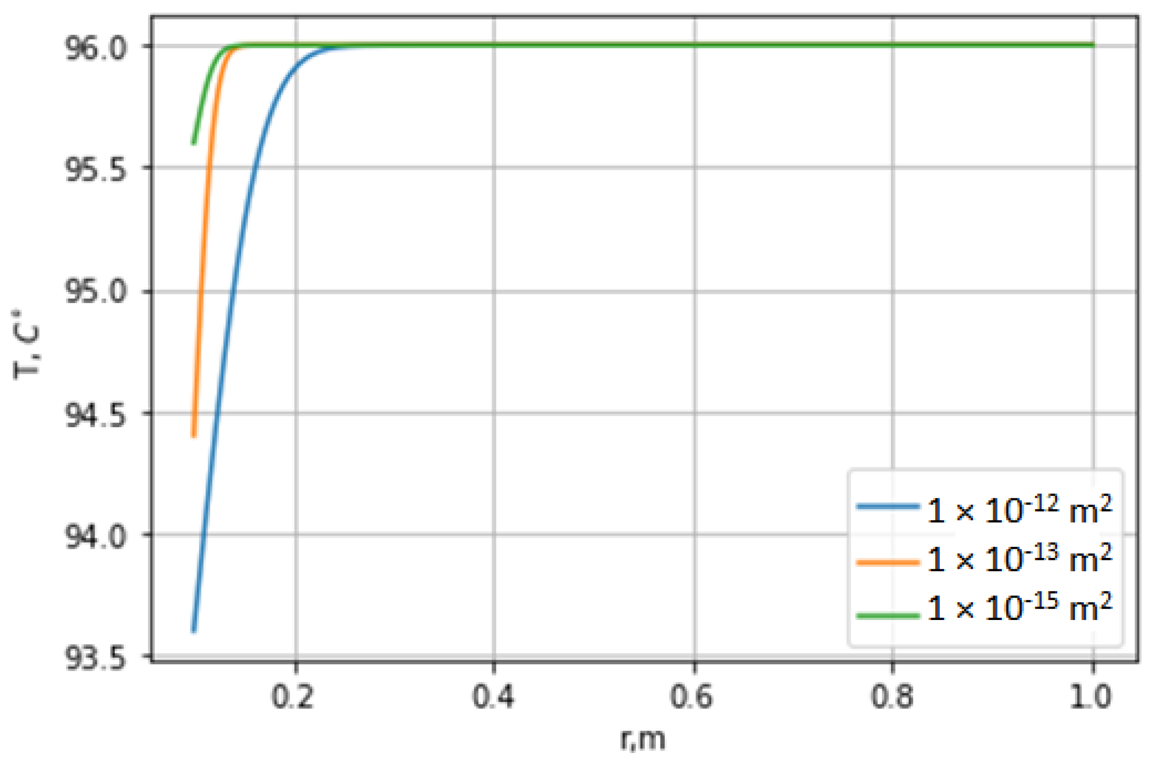
Figure 4 and Figure 5 show temperature versus time and distance, respectively. Note that the rate of temperature propagation in comparison with pressure is negligible. However, there is a difference. The radius of change in the temperature front will be slower than with pressure.

To study the properties of the matrix sweep parallelization algorithm and compare it with a sequential code, we use such characteristics as speedup coefficients $\left(S_m\right)$ and efficiency coefficients $\left(E_m\right)$.

$$S_m=\frac{T_1}{T_m},$$

(51)

$$E_m=\frac{S_m}{m}=\frac{T_1}{m·T_m},$$

(52)

where $S_m$ is the speedup, $E_m$ is the efficiency, $T_m$ is the execution time of the parallel program on m processes, and $T_1$ is the execution time of the sequential program.

Table 1. The speedup and efficiency of the parallel algorithm.

Number m of Processes	Speedup ${\mathit{S}}_{\mathit{m}}$	Efficiency ${\mathit{E}}_{\mathit{m}}$
1	1.0000	1.0000
4	3.3276	0.8319
8	4.8764	0.6095
10	5.9349	0.5934
12	7.1202	0.5933
14	7.9783	0.5699
16	8.9286	0.5580

shows the speedup and efficiency factors depending on the number of processes. We see that the speedup grows, and the efficiency decreases moderately.

The analysis of Table 1 showed that the matrix sweep algorithm accelerates the calculation time, which confirms the validity of using multiprocessor calculations for the problem under consideration.

6. Conclusions

The mathematical model of the mass transfer process taking into account the non-isothermal nature of a two-phase fluid in a fractured-porous reservoir based on a dual porosity model was developed. Based on the algorithm of splitting by physical processes, a difference scheme with time weights was constructed, which ensured the correctness and consistency of fluxes between the system of natural fractures and the pore reservoir. For the numerical solution of the problem, an original implicit finite-difference scheme on a spatial grid was proposed. The resulting system of equations was solved using a parallel matrix sweep algorithm. A series of computational experiments was carried out, the results of which confirmed the effectiveness of the developed numerical algorithm and its parallel implementation. Let us pay attention to the advantages of the proposed algorithm in comparison with a completely implicit scheme: three systems of equations of a smaller dimension were solved, instead of one. In all calculations, it was found that such an approach, when the system was split by physical processes, and the groups of equations were solved implicitly, ensured the reliability of the calculation in the investigated range of parameters and acceptable speed, which was quite suitable for solving practical problems. The calculated data were compared with field data; the error did not exceed 5%. The coefficients of speedup and efficiency for a different number of processes were presented. The optimal number of processes was obtained for fixed grid parameters. The result of the modeling was the distribution of pressure and temperature in a fractured-porous reservoir near an operating production well with varying permeability values in fractures. It was noted that the higher the permeability in the system, the faster the pressure dropped during the well operation. These calculations will allow us to monitor and regulate the work of wells in order to increase production.