Article

Multivariate Statistical and Correlation Analysis between Acoustic and Geotechnical Variables in Soil Compression Tests Monitored by the Acoustic Emission Technique

by
Gonzalo García-Ros
1,*,
Danny Xavier Villalva-León
1,
Enrique Castro
2,
Juan Francisco Sánchez-Pérez
2,
Julio Valenzuela
3 and
Manuel Conesa
2
1
Civil and Mining Engineering Department, Universidad Politécnica de Cartagena (UPCT), 30202 Cartagena, Spain
2
Applied Physics and Naval Technology Department, Universidad Politécnica de Cartagena (UPCT), 30202 Cartagena, Spain
3
Metallurgical and Mining Engineering Department, Universidad Católica del Norte, Antofagasta 1240000, Chile
*
Author to whom correspondence should be addressed.
Submission received: 11 August 2023 / Revised: 16 September 2023 / Accepted: 25 September 2023 / Published: 26 September 2023

Abstract

:
In this research, a series of compression tests were carried out, under oedometric conditions, on sand samples prepared with different moisture contents. In these tests, in addition to the usual measurements of the stress and deformation of the sample, a series of acoustic emission sensors were used to monitor the parameters of the acoustic signals coming from inside the sample. This is a rather novel technique with great potential, but sometimes difficult to approach due to the large amount of acoustic emission data generated. In this paper, a correlation and regression analysis has been performed to quantify the correlations between the geotechnical variables and the parameters characterizing the acoustic emissions. The results presented open an interesting horizon of possibilities since, as it has been shown, it is possible to determine the values of the geotechnical properties from the acoustic variables, by means of the regression functions obtained for each type of soil or for each practical case. At the very least, this is a complementary tool in the determination of the mechanical properties of soils subjected to compression, although it could also be useful in those situations in which the monitoring of geotechnical variables describing the tenso-deformational behavior of the soil may be difficult or impossible.

1. Introduction

Acoustic emissions are sound signals generated naturally or artificially by a source from different physical or mechanical processes [1,2]. They are detected and analyzed using specific devices and techniques [3,4,5], providing valuable information about the source itself or its environment in numerous disciplines and applications, such as geophysics [6], medicine [7], biology and zoology [8], machinery monitoring and mechanical engineering [9,10], and non-destructive inspection [11], among others.
Within the field of ground engineering, acoustic emissions are used for the monitoring and evaluation of soils and associated structural elements such as bridges [12], piles [13], dams [14], tunnels [15,16], and other infrastructure [3,17]. It is a non-destructive tool for detecting and analyzing the release of deformation energy in the form of acoustic waves [18], generated by a ground (or a supported structure) when subjected to loads, displacements, or mechanical stresses. It is a technique that is showing increasing progress within this discipline, as the early detection of any anomaly can be essential for the safety and integrity of constructions. Thus, this tool is proving very useful in works involving complex excavations [19], in slope stability assessments [20,21,22], where monitoring the energy associated with soil movement or fracturing [23] can be of great use in taking preventive measures, in geotechnical subsoil assessments [4,24], and in quality control and materials testing [25].
When a load or force is applied to a soil, its particles reorganize and compress [26,27], which can lead to microfractures or internal displacements [28] in the material that will release energy in the form of acoustic waves [29]. When these emissions are monitored, valuable information can be obtained about the evolution of soil deformation [28,30], changes in mechanical behavior [31,32], the location and propagation of microfractures [33], the presence of weaknesses or potentially unstable areas (of great importance for the safety assessment of structures built on the ground) [20], and, in general, the strength of the soil [29,34] to applied forces. Acoustic characteristics may vary according to the soil properties [33], applied load [13,26], and other factors [31], so specific equipment and knowledge [35], as well as a careful approach, are needed in each particular case.
For the analysis and processing of the large amount of acoustic emission data generated by sensors or capture devices, a widespread and very successful approach is their statistical treatment [36,37], allowing the extraction of relevant and meaningful information about the phenomena studied. The process includes several preliminary steps, such as cleaning and preparing the raw data for analysis (data pre-processing [38]) and obtaining descriptive statistics [39,40] to get a general idea of the distribution and variability of the data. Subsequently, depending on both the nature of the phenomena to be analyzed and the specific objectives of the study, techniques such as frequency analysis (amplitude or time domain) [41], correlation analysis [42], or trend and regression analysis [43,44] are commonly employed.
When working with large data sets generated by multiple sensors or measurement devices, multivariate analysis [45,46] can be applied to study the complex relationships that may exist between process variables (concentrations, pressures, displacements, deformations, stresses, etc.) and acoustic variables. The aim of multivariate statistical analysis is to identify patterns, trends, and correlations between the different variables (acoustic and self) in the process, which can provide a deeper and more detailed insight into the phenomena studied. Among the common techniques used in multivariate statistical analysis, we highlight correlation analysis [42], which is used to assess the relationship between two or more variables, helping to identify which variables are most strongly related and how they influence one another, and regression analysis [43,44], which is used to model the relationship between a dependent variable and one or more independent variables, allowing the value of one variable to be predicted as a function of the other related variables. Today, the use of specialized tools [47] and software [48,49] makes it easier to perform these complex and advanced statistical analyses on the data collected.
This paper presents an extensive statistical correlation analysis between the geotechnical variables (which characterize the mechanical behavior of a soil) of a series of sand samples subjected to compression tests and the parameters of the acoustic emissions that are generated, basically, because of the movement of grains and the frictional forces that develop in the contacts between particles. The organization and structure of this paper is as follows: Section 2 describes the tests carried out, the preparation of the samples, and the instrumentation used. The geotechnical and acoustic emission variables to be monitored during the tests are also defined. Subsequently, Section 3 explains how the data of the different variables were organized and processed, and Section 4 proceeds to the determination of the Pearson’s correlation coefficients and regression functions. This is followed by the graphical representation of these results. Section 5 contains an interesting discussion and, finally, Section 5 presents the main conclusions of this work.

2. Materials and Methods

2.1. Tests Performed

The study carried out includes compression tests on unsaturated sand samples in which, in addition to obtaining the classic stress–strain curves, sensors have been added to record the acoustic emissions (AE hereinafter) of the soil during its deformation. Specifically, the compression tests were carried out under oedometric conditions (no lateral deformations) and imposing a constant strain rate.
For these tests, the soil samples were subjected to a loading process, progressively increasing the vertical effective stress σ v from a preloading value (origin of the test) of 12.5 kN/m2 to a maximum value above 5000 kN/m2. To achieve this objective, the sample was deformed at a constant displacement rate of 1 mm/min. The loading process was subdivided into 9 stages, distributed as shown in Table 1. This discretization, similar to that of a conventional oedometer test (ASTM D2435 [50]), will facilitate the analysis and characterization of soil behavior for different stress levels. As can be seen, there is also a preloading stage, which is a preliminary phase with the objective of checking that both the sample and all the parts and sensors to be used during the test are correctly fixed and positioned.

2.2. Instrumentation

For the tests, an automated 50 kN press, as shown in Figure 1, was used, suitable for performing, among others, single uniaxial compression tests.
An electronic position transducer Gefran PY-2-C-010 (Gefran SPA, Brescia, Italy), with a resolution of 1 micron, was used to measure the shortening of the sample, while an electronic load cell (AEP transducers TS 1t C3, with a resolution of 0.1 N) was used to record the force exerted by the soil sample as resistance to the imposed deformation. The readings from both devices were collected by a data acquisition device Matest Cyber Plus Evolution A 8 Channels (Matest SpA, Bérgamo, Italy), which, at 1 s intervals, recorded and stored in a .txt file the data relating to the vertical deformation and resistance offered by the sample.
In addition, 2 low-frequency sensors, Vallen VS30-SIC-46 dB (Vallen Systeme GmbH, Wolfratshausen, Germany); frequency range 25–100 kHz, and 2 broadband sensors (Vallen VS900-RIC; frequency range 100–900 kHz) were used to record the AE events. The choice and use of these two types of sensors was intended to cover the frequency ranges of different internal soil processes. Thus, AEs below 100 kHz are usually associated with particle rearrangement, those between 100–200 kHz with abrasion of grain asperities, while above 200 kHz, the sand particles begin to show microcracking [31].
The 4 sensors were placed on the metal plate used to fix the oedometer ring (containing the soil sample inside) to the loading bench (Figure 2), surrounding the sample (at 90-degree angles) in order to better cover the AE events generated inside the soil (the provision of more sensors was not possible due to space limitations). The ultrasound generated inside the sample is picked up by the oedometer ring containing the soil, which transmits it directly to the metal plate on which the sensors rest. In this way, the sensors are located at no more than 3 cm from the origin of the AE. In addition, losses or attenuations at the sensor–plate and plate–ring contacts are minimal, on the one hand, because the plate–ring contact occurs along the entire lateral surface of the ring, as well as being completely watertight; on the other hand, the base of the sensors (where they detect the AE) is impregnated with a gel that guarantees perfect coupling between the metal plate and the sensor, minimizing losses.
The AE events captured by the sensors are sent to a multi-channel AE recording system (Vallen AMSY-6 System). This device, together with the help of specific software (Vallen VisualAE R2021.1122.1), allows the analysis and processing of the recorded AE data, based on their different characteristics: hits number, amplitude, duration, counts, frequency, rise time, and energy, among others. The time interval between recordings is set automatically, each time a sensor recognizes an AE hit.
Preliminary tests were carried out to determine the amplitude threshold above which AE were not recorded when the soil was not being subjected to the compression process; that is, placing the soil inside the oedometer ring and the loading equipment, but without any stress being applied (in this state, we know for sure that the sample is not emitting any ultrasound). This threshold ranged between 38 and 39 dB for the different preliminary tests. Finally, the multi-channel AE recording system was set to a threshold of 40 dB for the final tests.

2.3. Samples Used: Test Preparation and Procedure

For the compression and EA tests of this study, coastal sand from the Mar Menor (S.E. Spain) shore, with mostly rounded grains and with a size range between 0.075 and 2 mm, was used. Although their presence in the original samples was very low, diameters larger than 2 mm and smaller than 0.075 mm were removed from the sample by sieving. Sizes smaller than 0.075 mm may have some chemical affinity for the added water, and for this first contact with the technique, we wanted to rule out this effect. On the other hand, sizes larger than 2 mm were very rare in the original sand, so their presence in the tested samples of about 60–80 g had no place.
For the correct identification and classification of the samples finally used, they were first washed, dried, and finally sieved. Initially, subsamples with the following size ranges were obtained: R1 = 0.075–0.106 mm, R2 = 0.106–0.2 mm, R3 = 0.2–0.3 mm, R4 = 0.3–0.4 mm, R5 = 0.4–0.6 mm, R6 = 0.6–0.8 mm, R7 = 0.8–1.4 mm, and R8 = 1.4–2 mm. The weight percentages of each size range were quite close to those finally selected. Thus, the samples finally tested were obtained from the following mixture:
Ss = R1 (11.1%) + R2 (11.1%) + R3 (11.1%) + R4 (16.6%) + R5 (16.6%) + R6 (11.1%) + R7 (11.1%) + R8 (11.1%).
In order to guarantee the exact value of the moisture content ω c in each sample, a new drying process was initially carried out for the subsequent addition of the water content: 0% (dry sand), 3%, 6%, 9%, and 12%. Prior to being tested, the samples were subjected to a compaction process by applying a vibration (of medium intensity) at the same time as they were poured inside the oedometric ring. It should be noted that for the dry sand ( ω = 0%), both a vibrated sample (V) and a loose sample with no vibration (L) were prepared, although in the end, both samples presented very similar compaction values. For all the samples, their mechanical characteristics’ initial void ratio e 0 and initial dry density ρ d , 0 were obtained (Table 2).
The oedometric ring (rigid and containing the sample inside) has the following inner dimensions: height, H 0 = 20 mm; diameter, ϕ i n t = 50 mm.

2.4. Geotechnical Properties of the Soil

At the beginning and during the compression tests, a series of mechanical properties were monitored, thanks to the processing of the data coming from the position transducer and the load cell (both electronic). These properties provide valuable information on the state of the soil: moisture, density, void ratio (porosity), stress level, compressibility, and deformation.
Before setting out the mechanical properties monitored (after defining a number of basic properties) for this study, it is necessary to establish a couple of reference points (or states) for our tests:
  • Test beginning, point 0. We will refer to this point when referring to the state of the soil prior to the application of any load (vertical effective stress σ v = 0 kN/m2). It corresponds to the state of the soil after preparation (drying and addition of moisture content), placement and compaction in the oedometric ring. In this state, the sample has not yet undergone any deformation or increase of its internal stress.
  • Test origin, point o. After placing the sample in the test press, the soil is slightly preloaded at a vertical effective stress, σ v = 12.5 kN/m2, to check that both the sample and all the parts and sensors to be used during the test are correctly positioned and fixed. Logically, in this state, the sample has shown some deformation, as well as an increase in its internal stress ( σ v ).

2.4.1. Definition of Basic Soil Properties

  • Sample thickness, H (mm). The height of the soil sample within the oedometric ring, which decreases as the applied load increases. Its initial value for all the samples tested is H 0 = 20 mm.
  • Sample volume, V (cm3). The volume of the soil sample within the oedometric ring, which decreases as the applied load increases. Its initial value for all the samples tested is V 0 = H 0 S = H 0 π ϕ i n t 2 / 4 = 39.27 cm3. Furthermore, it is always true that the total volume V of the sample is equal to the sum of the volume of solids V s and the volume of voids V v .
  • Strain, ε i . Ratio between the deformation and the original length of the sample in axial direction at a given instant i. Since the sample cross-section is constant, it can be defined both in terms of the initial volume ( V 0 ) and the initial thickness ( H 0 ). It is obtained from the following expression (taking compression as a deformation of positive sign):
    ε i = ( H ) i H 0 = H i H 0 H 0 = V i V 0 V 0 = ( V ) i V 0
  • Solids volume, ( V s ) (cm3). Volume occupied exclusively by solid soil particles.
  • Voids volume, ( V v ) (cm3). The volume of the space between particles. It may be occupied by air, water, or a combination of both.
  • Void ratio, e . Ratio between the voids volume and the solids volume.
    e = V v V s
  • Dry mass of the soil, m d (g). The mass of the soil sample after removal of all the water m a it contains (by drying in an oven at 60 °C for 24 h).
  • Mass of water, m a (g). Mass of water contained in the soil, prior to its removal by drying in an oven at 60 °C for 24 h.
  • Specific gravity of the soil particles, G s . Ratio of density of solid particles to density of water. For our soil, this intrinsic parameter never changes and has a value of 2.78.
The determination of the latter parameter (using the pycnometer method, ASTM D854-14 [51]) greatly facilitates the monitoring of the void ratio e since, by means of the expression e = G s ρ w / ρ d 1 , it is directly related to the dry density of the soil ( ρ d = m d / V ), not being necessary to determine the volumes V v and V s . In this way, the monitoring of the sample strain ε i , thanks to the electronic position transducer (Gefran PY-2-C-010), makes it possible to always know the thickness of the sample H and, therefore, its volume ( V = H S). On the other hand, after finishing each compression test, the sample is weighed, before and after 24 h in the drying oven at 60 °C, so that the total mass of the sample, the mass of water m a , and the dry mass of the soil m d are obtained.

2.4.2. Geotechnical Properties Monitored

Both at the beginning and during the 9 loading stages (Table 1), into which each test was subdivided, the following geotechnical variables were monitored and computed.
  • Moisture content, ω c (%). Ratio between the mass of water and the dry mass of the soil.
    ω c = m a m d
    Five possible values for vibrated samples: ω 0 , v = 0%; ω 3 , v = 3%; ω 6 , v = 6%; ω 9 , v = 9%; ω 12 , v = 12%, plus one value for the loose sample: ω 0 , l = 0%, as shown in Table 2.
  • Initial dry density, ρ d , 0 (g/cm3). Ratio of the dry mass of the soil (without moisture) to its initial volume:
    ρ d , 0 = m d V 0
One different value for each test carried out (Table 2).
  • Initial void ratio, e 0 . Ratio between the initial volume of voids ( V v , 0 ) and the volume of solids ( V s ). One different value for each test carried out (Table 2). It can be obtained from the following expression:
    e 0 = G s ρ w ρ d , 0 1
    where G s is the specific gravity of the soil particles and ρ w is the density of the water.
  • Loading stage effective stress, σ l s (kN/m2). Nine different values, represented by the effective stress reached by the soil at the end of each loading stage (Table 1):
    σ 25 = 25 kN/m2; σ 50 = 50 kN/m2; σ 100 = 100 kN/m2; σ 200 = 200 kN/m2; σ 400 = 400 kN/m2; σ 800 = 800 kN/m2; σ 1600 = 1600 kN/m2; σ 3200 = 3200 kN/m2; and σ 5000 > 5000 kN/m2.
  • Loading stage density, ρ d , l s (g/cm3). Ratio of the dry mass of the soil (without moisture) to its volume at the end of a loading stage.
    ρ d , l s = m d V l s
    Thus, there are 9 variable values for each test carried out: ρ d , 25 (for loading stage 1, Table 1), ρ d , 50 (for loading stage 2, Table 1), and so on for ρ d , 100 , ρ d , 200 , ρ d , 400 , ρ d , 800 , ρ d , 1600 , ρ d , 3200 , and ρ d , 5000 .
  • Loading stage void ratio, e l s . Ratio between the volume of voids at the end of a loading stage ( V v , l s ) and the volume of solids ( V s ). It can be obtained from the following expression:
    e l s = G s ρ w ρ d , l s 1
    Nine variable values for each test carried out, defined similarly to the above: e 25 , e 50 , e 100 , e 200 , e 400 , e 800 , e 1600 , e 3200 , and e 5000 .
  • Loading stage compression index, c c , l s . Slope of the e - log 10 σ curve between the start and end points of a given loading stage. It is obtained from the following expression:
    c c , l s = e f , l s e o , l s log 10 ( σ f , l s σ o , l s )
    where the subscripts o,ls and f,ls refer to the start and end points of a given loading stage. Thus, there are nine variable values, defined similarly to the above: c c , 25 , c c , 50 , c c , 100 , c c , 200 , c c , 400 , c c , 800 , c c , 1600 , c c , 3200 , and c c , 5000 .
  • Loading stage strain, ε l s . Strain of the sample at the end of a loading stage:
    ε l s = ( H ) l s H 0 = H l s H 0 H 0 = V l s V 0 V 0 = ( V ) l s V 0
    Nine variable values for each test carried out, defined similarly to ρ d , l s . ε 25 , ε 50 , ε 100 , ε 200 , ε 400 , ε 800 , ε 1600 , ε 3200 , and ε 5000 .
  • Loading stage coefficient of compressibility, a v , l s (m2/kN). Slope of the curve relating the void ratio ( e ) to the effective stress ( σ ) between the start and end points of a given loading stage. It is obtained from the following expression:
    a v , l s = e f , l s e o , l s σ f , l s σ o , l s
    Nine variable values, equally conceived as c c , l s : a v , 25 , a v , 50 , a v , 100 , a v , 200 , a v , 400 , a v , 800 , a v , 1600 , a v , 3200 , and a v , 5000 .

2.5. Parameters and Characteristics of Acoustic Emissions

Each of the AE events inside the sample, captured by the 4 AE sensors, is sent as an electrical signal to the multi-channel AE recording system (channels 1 and 3 for the broadband sensors; channels 2 and 4 for the low-frequency sensors) which interprets it to obtain a typical transient signal waveform (Figure 3), from which the main properties and characteristics of the AE are obtained. These are briefly described below.

2.5.1. Definition of Basic Characteristics of Acoustic Emissions

  • Hit. Acoustic emission event that is sensed by a sensor and whose signal is sent for processing to the multi-channel AE recording equipment, resulting in a waveform, as in Figure 3.
  • Hits number, N H i t . During a given time interval (or process or test), the number of total hits that are sensed by the AE sensors and subsequently stored and processed in the multi-channel AE recording system.
  • (Peak) Amplitude, A (dB). Maximum amplitude (height) that the wave reaches with respect to the horizontal axis. It is usually expressed in decibels (dB), although the real output signal from the AE sensor has units of electrical potential. The equivalence is given by the following expression:
    A = 20 log 10 ( V s e n s o r )
    where V s e n s o r is the maximum electrical potential sensed by the AE sensor for a given hit, expressed in µV.
  • Threshold (dB). Positive lower limit (or minimum value) that the amplitude of the AE signal must have. It is used to filter and discard those AE signals that do not exceed this value, in order to eliminate unwanted hits or noise. For the tests carried out in this research, the threshold established was 40 dB.
  • Counts number, C N T S . Number of crossings of the positive threshold.
  • Signal Duration, D (µs). Time interval between the first and the last time the positive threshold is crossed.
  • Frequency, F (kHz). Average counts number per unit of time. This is:
F = C N T S D
  • Rise time, R T (µs). Time interval between the first time the positive threshold is exceeded and the time when the peak amplitude is reached.
  • Energy, E (aJ). Integral (area under the curve) of the squared amplitude over the signal duration time. It is usually expressed in energy units (eu), 1 eu = 10−18 J = 1 aJ.
In addition, a couple of statistical parameters derived from the AE data are proposed for the assessment of the AE in our compression tested soils:
  • b value, b . Slope of the relation between the decimal logarithm of the number of hits that exceed a given amplitude ( log 10 N H i t A ) to the decimal logarithm of that amplitude ( log 10 A ). If we consider two consecutive points, its expression is:
    b = log 10 ( N H i t A , i N H i t A , i 1 ) log 10 ( A i A i 1 )
    where N H i t A , i is the number of hits that exceed the amplitude A i [52,53].
  • r value, r (1/aJ). Ratio between the cumulative number of hits (of a given process) and their cumulative energy. Qualitatively, it is expressed by the following equality:
    r = N H i t E

2.5.2. Acoustic Emission Properties Monitored

For each of the 9 loading stages (Table 1) into which each test was subdivided, the following acoustic variables were monitored and computed.
  • Loading stage hits number, N H i t l s . The total number of hits recorded in a loading stage. Nine variable values:
    N H i t 25 (for the loading stage between σ f , l s around 25 kN/m2 and σ o , l s around 12.5 kN/m2), and so on for N H i t 50 , N H i t 100 , N H i t 200 , N H i t 400 , N H i t 800 , N H i t 1600 , N H i t 3200 , and N H i t 5000 .
  • Loading stage amplitude, A l s (dB). Average amplitude of the hits of a given loading stage.
    A l s = i = 1 i = N H i t l s A i N H i t l s
    where A i represents the amplitude of a single instant hit of the loading stage of ls. Defined similarly to ρ d , l s , A 25 , A 50 , A 100 , A 200 , A 400 , A 800 , A 1600 , A 3200 , and A 5000 are the nine variable values for this parameter.
    In our sand compression process, the signal amplitude gives an idea (or measure) of the magnitude of the friction and microcracking phenomena. Thus, a higher amplitude implies larger microcracks, or a greater intensity of friction. In addition, when working with different materials, the more resistant ones usually present higher amplitudes. However, this is not our case since the sand samples are homogeneous in nature.
  • Loading stage signal duration, D l s (µs). Average signal duration of the hits of a given loading stage.
    D l s = i = 1 i = N H i t l s D i N H i t l s
    where D i represents the signal duration of a single instant hit of the loading stage of ls. Defined similarly to the above, D 25 , D 50 , D 100 , D 200 , D 400 , D 800 , D 1600 , D 3200 , and D 5000 are the nine variable values for this parameter.
    The signal duration gives a direct measure of how long in time the process that generates the ultrasound is. However, it must be taken into account that its value is greatly influenced by the peak amplitude, since for those emissions with higher amplitudes, its associated wave takes longer to attenuate (longer time for the last crossing of the positive threshold).
  • Loading stage counts number, C N T S l s . Average counts number of the hits of a given loading stage.
    C N T S l s = i = 1 i = N H i t l s C N T S i N H i t l s
    where C N T S i represents the counts number of a single instant hit of the loading stage of ls. Defined similarly to the above, C N T S 25 , C N T S 50 , C N T S 100 , C N T S 200 , C N T S 400 , C N T S 800 , C N T S 1600 , C N T S 3200 , and C N T S 5000 are the nine variable values for this parameter.
  • Loading stage frequency, F l s (kHz). Average frequency of the hits of a given loading stage.
    F l s = i = 1 i = N H i t l s F i N H i t l s
    where F i represents the frequency of a single instant hit of the loading stage of ls. Defined similarly to the above, F 25 , F 50 , F 100 , F 200 , F 400 , F 800 , F 1600 , F 3200 , and F 5000 are the nine variable values for this parameter.
    The magnitude of the frequency is linked to the greater or lesser speed of development of the internal physical phenomena occurring in the material. Thus, sudden processes such as the appearance of microcracks present higher frequencies than other more gradual phenomena such as particle rearrangement or abrasion of grain asperities.
  • Loading stage rise time, R T l s (µs). Average rise time of the hits of a given loading stage.
    R T l s = i = 1 i = N H i t l s R T i N H i t l s
    where R T i represents the rise time of a single instant hit of the loading stage of ls. Defined similarly to the above, R T 25 , R T 50 , R T 100 , R T 200 , R T 400 , R T 800 , R T 1600 , R T 3200 , and R T 5000 are the nine variable values for this parameter.
  • Loading stage energy, E l s (aJ). Average energy of the hits of a given loading stage.
    E l s = i = 1 i = N H i t l s E i N H i t l s
    where E i represents the energy of a single instant hit of the loading stage of ls. Defined similarly to the above, E 25 , E 50 , E 100 , E 200 , E 400 , E 800 , E 1600 , E 3200 , and E 5000 are the nine variable values for this parameter.
    The AE wave energy gives us a measure of the energy released by the rearrangement, abrasion, and microcracking phenomena that occur in the material during compression.
  • Loading stage b value, b l s . Slope of the regression line relating the decimal logarithm of the number of hits (of a given loading stage) that exceed a given amplitude ( log 10 N H i t A ) to the decimal logarithm of that amplitude ( log 10 A ), Equation (13). Nine variable values for this parameter, defined in similar terms to the variables above: b 25 , b 50 , b 100 , b 200 , b 400 , b 800 , b 1600 , b 3200 , and b 5000 .
  • Loading stage r value, r l s (1/aJ). Ratio of the loading stage hits number N H i t l s to their cumulative energy. It can be defined through the following expression:
    r l s = N H i t l s E l s N H i t l s = 1 E l s
    Defined in similar terms to the above, we have nine variable values for this parameter: r 25 , r 50 , r 100 , r 200 , r 400 , r 800 , r 1600 , r 3200 , and r 5000 .

3. Processing of Acoustic Emission and Geotechnical Data

Figure 4 shows a flow chart outlining how the processing of both geotechnical and acoustic emission data was carried out. In the following, we proceed to describe how these processes went.

3.1. Geotechnical Data Processing

The sample shortening and compressive strength data were sent to the acquisition device (Matest Cyber Plus Evolution A 8 Channels), which generates a .txt file for each test performed to store the data. The preconfiguration of this device led to data being available at 1 s intervals.
These text files were then loaded and manipulated with Python to obtain the values of the monitored geotechnical variables (defined in Section 2.4.2), which are summarized in Table 3.

3.2. Acoustic Emission Data Processing

The AE events captured by the four sensors were sent to and recorded by the multi-channel AE recording (Vallen AMSY-6) system. For viewing and processing, the Vallen VisualAE R2021.1122.1 software was used, which allows, among a wide range of tools, to apply filters (by amplitude, frequency, duration, counts, energy, etc.) on the recorded acoustic emissions to eliminate unwanted events or noise.
However, after a series of initial noise tests, it was determined that the 40 dB threshold worked efficiently in filtering and eliminating the noise generated by the laboratory environment and the test equipment itself, so no additional filtering was necessary in this sense.
The only filter used is a tool provided by the software that allows identifying those hits that correspond to the same AE event. This happens when the same AE event is picked up by several sensors, so that we have a different hit for each sensor that has sensed the same event. This tool was applied with the criterion of keeping the first (in time) of the hits recorded for the same event, discarding those that were recorded later (which, presumably, were further away from the source, thus suffering greater attenuation).
Finally, all the AE data were then loaded and manipulated with Python to obtain the values of the monitored acoustic emission variables (defined in Section 2.5.2), which are summarized in Table 4.

3.3. Data Organization

3.3.1. Fixed Value of Moisture Content

In this case, the data were classified into six different files, separately, according to the moisture content ω c . In other words, these are the data obtained for each of the six tests carried out (Table 2), in which, in addition, both the initial dry density ρ d , 0 and the initial void ratio e 0 also have fixed values.

3.3.2. Any Value of Moisture Content

In this case, the data were unified in one single file, so that in its subsequent analysis it will be possible to evaluate the influence that the moisture content ω c , the initial dry density ρ d , 0 , and the initial void ratio e 0 have on the properties of the AEs. However, it is important to clarify that, for this assumption, the data from sample ID = 1 (in Table 2  ω c = 0% and without vibration) were not taken into account. The reason is so as to not mix data from five vibrated soils with data from one non-vibrated soil, as this could lead to erroneous conclusions about one soil type and the other. Therefore, this analysis will be limited to vibrated soils only.

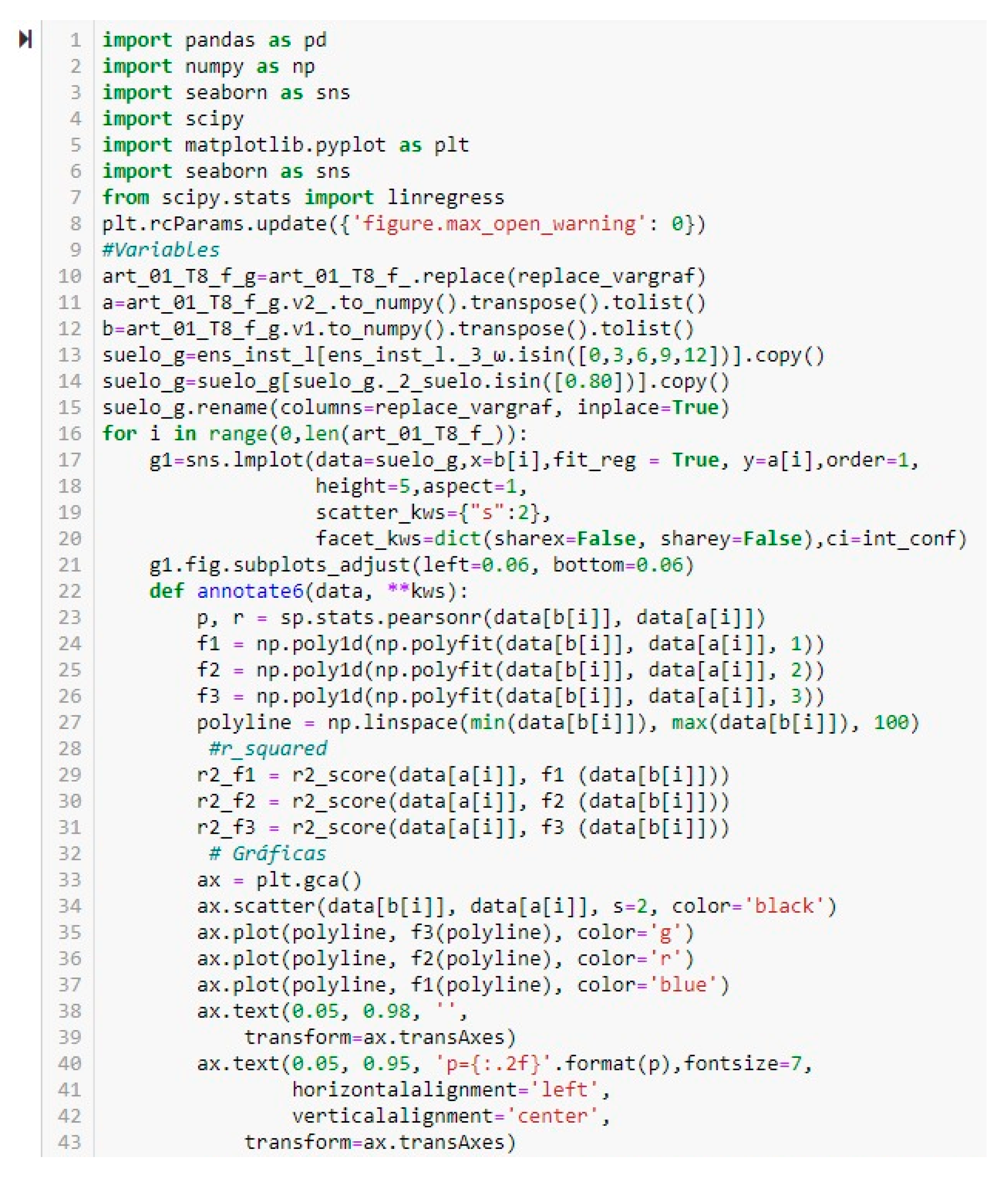
3.4. Functions and Operations with Python

By default, Python 3.11.5 (https://www.python.org/) incorporates a wide variety of resources and tools in its installation version. However, it was necessary to import some additional libraries to perform correlation and regression analyses between geotechnical and acoustic variables, as well as for their graphical representation. Thus, to obtain the Pearson correlation coefficient, p, the function stats.pearsonr (from the scipy library) was used, while for the regression analysis, polynomial adjustments (of orders 1, 2, and 3) and graphical representations, functions such as lmplot and polyfit (belonging, respectively, to the seaborn and numpy libraries), were used. Figure 5 shows an important part of the code, where the aforementioned functions are used.

4. Pearson’s Correlation Coefficients and Regression Functions

This section presents the results of the statistical analyses carried out, which are summarized below:
-
Pearson’s correlation coefficients, p, between geotechnical and acoustic variables.
-
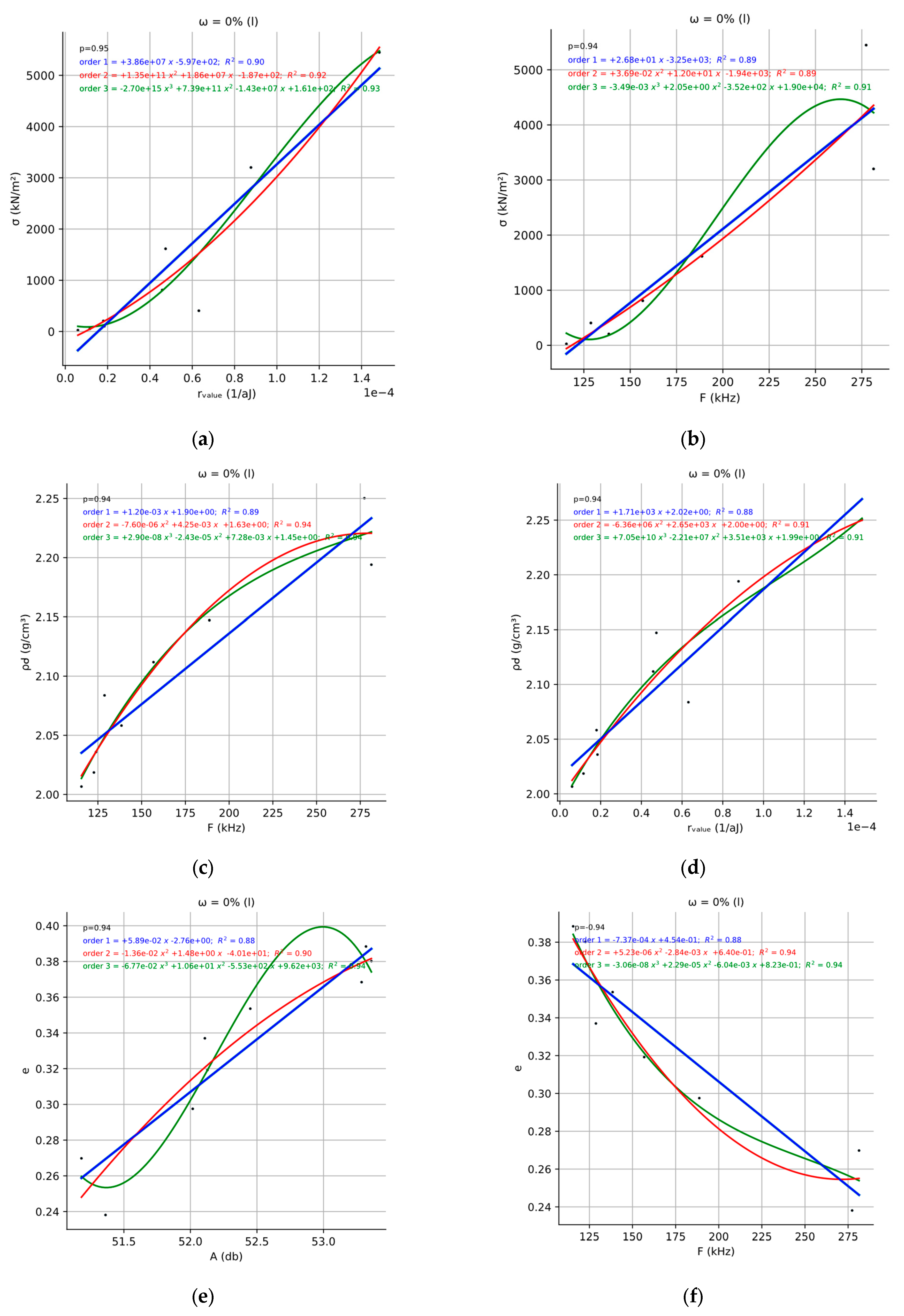
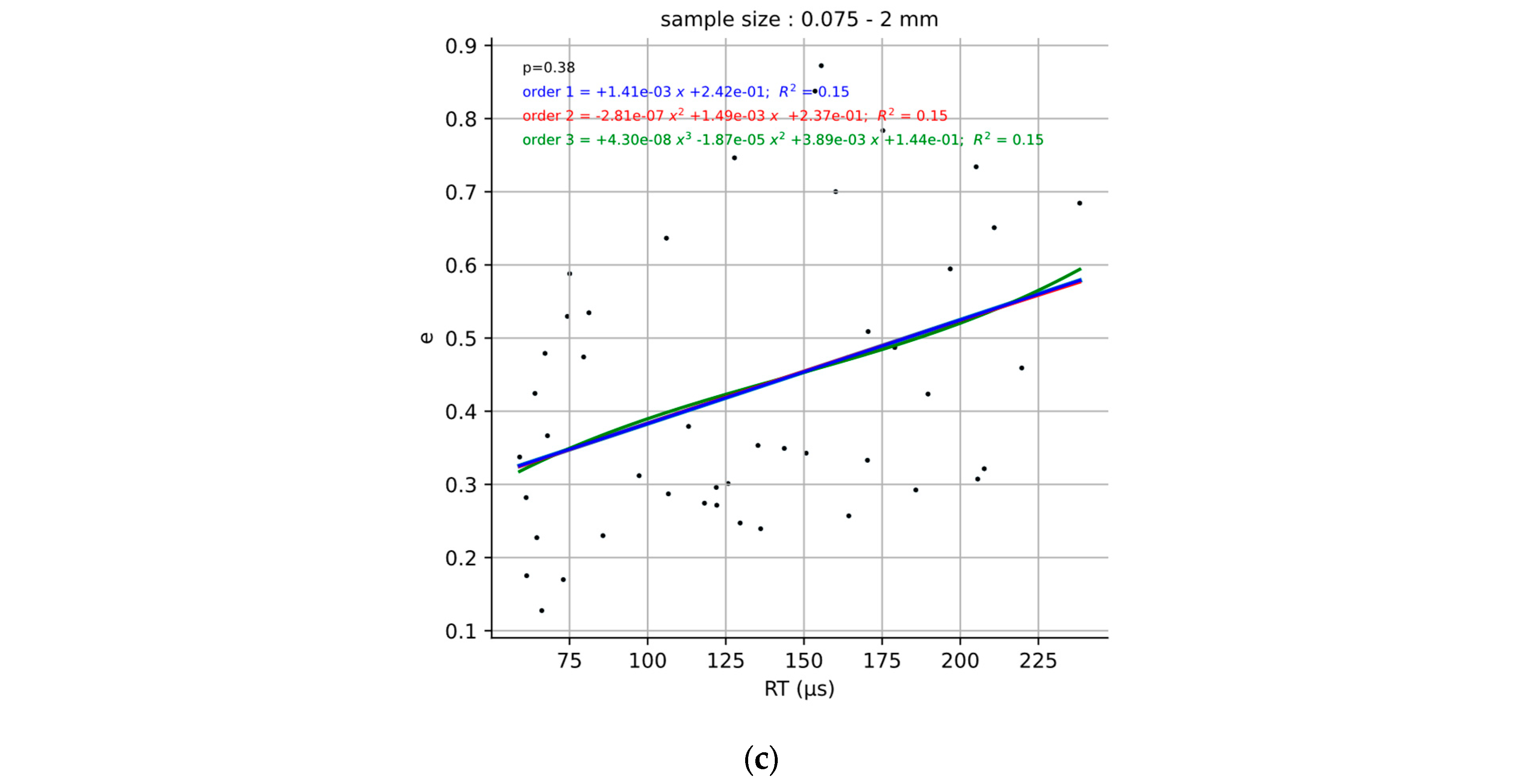
Polynomial regression functions (order 1, 2, and 3) obtained by the least-squares fitting method.
-
Graphical representations of the regression functions, indicating both the Pearson’s correlation coefficient p and the coefficient of determination R2.
As explained in Section 3.3, the analysis was carried out from a double perspective: firstly, analyzing each of the six tests carried out separately (fixed value of moisture content); secondly, jointly analyzing the data from the six tests (any value of moisture content), which will allow (additionally) to evaluate the influence that the moisture content ω c , the initial dry density ρ d , 0 , and the initial void ratio e 0 have on the properties of the AEs.
In reality, correlation and regression analysis were also possible between two geotechnical variables, or between two acoustic variables. However, as the final objective of this research was to be able to infer (in a hypothetical real case) the values of the geotechnical variables from the monitoring of acoustic emissions, these correlations have been eliminated from the analysis.

4.1. Analysis for Fixed Values of Moisture Content

For this assumption, since the values of ω c , ρ d , 0 , and e 0 are constant for each test, it is only possible to perform a correlation analysis for the geotechnical variables σ l s , ρ d , l s , e l s , c c , l s , ε l s , and a v , l s (Table 3).
Table 5 shows the three acoustic variables that best correlate with the six geotechnical variables above: σ l s , ρ d , l s , e l s , c c , l s , ε l s , and a v , l s . For each acoustic variable, the two soils (out of the total of six) with the best p values ( p 1 s t and p 2 n d , respectively) are shown.
The functions and regression lines of the two acoustic variables that best correlate with σ l s , ρ d , l s , and e l s are shown in Figure 6, while for variables c c , l s , ε l s and a v , l s , in Figure 7. In this case, only the soil with the best correlation, p 1 s t , is shown.
Finally, the functions and regression lines of the three acoustic variables that best correlate with σ l s , ρ d , l s , e l s , c c , l s , ε l s , and a v , l s can be found in the Supplementary Materials (Figures S1–S18). In this case, the graphs for the six tested soils are presented.

4.2. Analysis for Any Value of Moisture Content

For this case, it was possible to perform the correlation analysis for all monitored geotechnical variables in Table 3: ω c , ρ d , 0 , e 0 , σ l s , ρ d , l s , e l s , c c , l s , ε l s , and a v , l s . Recall that, for this analysis, the data from sample ID = 1 (in Table 2  ω c = 0% and without vibration) were not considered. Therefore, this analysis is limited to the five vibrated soils only.
Thus, Table 6 shows, in principle, the five monitored acoustic variables (Table 4) that best correlate with the above geotechnical variables. However, it should be noted that a lower limit has been imposed for the Pearson’s correlation coefficient, p ≥ 0.30, in order to eliminate the weakest correlations. Therefore, for some geotechnical variables, the number of correlations with the acoustic variables presented in Table 6 is lower than five. In addition, a column has been added to the table describing the degree of correlation, according to the following criteria [54,55]: perfect for p = 1; very high for 1 > p ≥ 0.8; high for 0.8 > p ≥ 0.6; moderate for 0.6 > p ≥ 0.4; low for 0.4 > p ≥ 0.2; very low for 0.2 > p > 0; and no correlation for p = 0.
Figure 8, Figure 9 and Figure 10 present the functions and regression lines for the best correlations found for each of the monitored geotechnical variables.
Finally, the functions and regression lines for the three (or two) best correlations for each geotechnical variable shown in Table 6 can be found in the Supplementary Materials (Figures S19–S27).

5. Discussion of Results and Conclusions

From the analysis for the fixed values of the moisture content, we observe the existence of very high correlations between the geotechnical and acoustic variables. Thus, for every one of the geotechnical variables ( σ l s , ρ d , l s , e l s , c c , l s , ε l s , and a v , l s ), the presence of more than one correlation with the Pearson’s coefficient, in absolute value p , above 0.90 is detected (Table 5), sometimes reaching values of 0.97, as is the case for the correlation c c , l s r l s . In most cases, the acoustic variables that correlate best with the geotechnical variables are r l s , F l s , and A l s , which highlights the special attention that should be paid to these properties when monitoring and interpreting the AEs generated by a soil under compression, since a quality estimation of the geotechnical variables from the regression functions would depend on the accuracy of these measurements.
As regards the loading stage frequency, F l s , this variable has presented a positive correlation with the loading stage effective stress, σ l s . This implies that higher stress states will lead to higher frequency acoustic emissions, showing the evolution between the different internal mechanisms that occur during compression [31], that is: for low and medium stress levels, the soil will undergo particle rearrangement and the abrasion of asperities, processes that generate acoustic emissions at frequencies below 200 kHz, while at high stress levels, the sand particles begin to show microcracking, generating AE waves whose frequencies are above 200 kHz.
Likewise, the loading stage frequency, F l s , also shows positive correlations with the variables’ loading stage density, ρ d , l s , loading stage compression index, c c , l s , and loading stage strain, ε l s . Its physical interpretation is similar to the above: the denser and more compressed the soil, the higher the frequencies and the more important the microcracking process. On the other hand, the loading stage void ratio, e l s , is negatively correlated with F l s , and this is due to the inverse relationship it has with density (when a soil is compressed, its density increases, thus decreasing the volume of voids).
As for the loading stage r value, r l s , this acoustic variable shows very similar correlations and trends to the loading stage frequency, F l s . This presents us with a very interesting conclusion, since an increase in the value of r l s implies a higher number of high-energy AE events [24], i.e., events related to microcracking processes at high stress levels.
Finally, as for the loading stage amplitude, A l s , its trends and correlations are always of an opposite sign to those of F l s and r l s . However, the variation intervals of this variable are too narrow, with an almost constant value in the range of 50–53 dB. For this reason, we consider that this property should play a less relevant role when estimating the geotechnical variables from the regression functions.
Furthermore, it has been observed that the sample prepared with a moisture content ω c = 0% and with no vibration is the one with the best correlations, although, as shown in Table 5, the other samples (all of them vibrated; ω c = 0%, 3%, 6%, 9%, 12%) also present high degrees of correlation, with p above 0.87. Undoubtedly, the fact that the only sample that was not subjected to vibration showed the highest correlations opens the door to the extension of this research, probably with these same samples, but also with others that are prepared with different moisture contents and without vibration, with alternative compaction methods or even with different particle sizes.
On the other hand, the joint analysis of all the data, with no restrictions for the moisture content value, has made it possible to obtain correlations with all the geotechnical variables in Table 3. That is, not only σ l s , ρ d , l s , e l s , c c , l s , ε l s , and a v , l s , but also ω c , ρ d , 0 , and e 0 . In this case, the values of Pearson’s correlation coefficient are lower than the previous assumption, but now 45 data are correlated, instead of 9. This undoubtedly gives a greater robustness to the regression functions obtained, despite the lower p values. Nevertheless, high degrees of correlation ( p above 0.60) have been found for the geotechnical variables c c , l s and ε l s , with the correlation ε l s r l s having the highest value, p = 0.77. On the other hand, the geotechnical variables ω c , σ l s , ρ d , l s , and a v , l s present moderate degrees of correlation (0.6 > p ≥ 0.4) with the acoustic variables, so that the resulting regression functions will also allow us to infer the values of the geotechnical variables, although with some caution. In this group, particularly interesting is the negative correlation σ l s D l s (or the similar σ l s R T l s ), which shows that at higher stress levels, the processes occurring inside the sample, such as microfractures, become shorter in time. Finally, the variables ρ d , 0 , e 0 , and e l s show low degrees of correlation ( p below 0.40).
As for the regression functions, from the point of view of the R2 value, the polynomial fit of order three will always be the best, followed by that of order two and leaving order one (linear) in last place. This is logically due to the greater geometrical flexibility offered by polynomials of order two (parabolic form) and order three (possibility of including an inflection point) compared to the straight line provided by the linear fit. In general, and in view of our results, this will always be the case, especially in those data sets in which the degree of correlation is high (0.8 > |p| ≥ 0.6) or very high (1 > |p| ≥ 0.8), in which the form described by the cubic regression function is observed to fit the real data set very well. Perhaps this statement can also be extended to those cases with a moderate degree of correlation and whose |p| is above 0.5.
However, it is observed that when the degree of correlation is low (or moderate, but with |p| below 0.5), the three polynomial fits tend to present very similar forms, yielding close R2 values. Therefore, for these cases, perhaps the best option is the linear-type fit, due to the greater simplicity of its mathematical expression.
In conclusion, from the correlation and regression analyses carried out for the numerous geotechnical and acoustic variables monitored during the oedometric compression tests, it follows that it is possible to infer, or at least estimate, the values of the geotechnical variables from the monitoring and analysis of acoustic emissions generated by the soil during its deformation.
Therefore, the acoustic emission technique is presented as a complementary tool in the determination of the mechanical properties of soils subjected to compression and can even be very useful in those situations in which it is not possible to monitor the geotechnical variables that describe the tenso-deformational behavior of the soil.

Supplementary Materials

The following supporting information can be downloaded at: https://0-www-mdpi-com.brum.beds.ac.uk/article/10.3390/math11194085/s1, Figure S1: Regression lines for the correlation between loading stage effective stress ( σ l s ) and loading stage r value r l s . Six soils tested, (a) ω c = 0%; (b) ω c = 0% (L); (c) ω c = 3%; (d) ω c = 6%; (e) ω c = 9%; (f) ω c = 12%; Figure S2: Regression lines for the correlation between loading stage effective stress ( σ l s ) and loading stage frequency F l s . Six soils tested, (a) ω c = 0%; (b) ω c = 0% (L); (c) ω c = 3%; (d) ω c = 6%; (e) ω c = 9%; (f) ω c = 12%; Figure S3: Regression lines for the correlation between loading stage effective stress ( σ l s ) and loading stage amplitude A l s . Six soils tested, (a) ω c = 0%; (b) ω c = 0% (L); (c) ω c = 3%; (d) ω c = 6%; (e) ω c = 9%; (f) ω c = 12%; Figure S4: Regression lines for the correlation between loading stage density ρ d , l s and loading stage frequency F l s . Six soils tested, (a) ω c = 0%; (b) ω c = 0% (L); (c) ω c = 3%; (d) ω c = 6%; (e) ω c = 9%; (f) ω c = 12%; Figure S5: Regression lines for the correlation between loading stage density ρ d , l s and loading stage r value r l s . Six soils tested, (a) ω c = 0%; (b) ω c = 0% (L); (c) ω c = 3%; (d) ω c = 6%; (e) ω c = 9%; (f) ω c = 12%; Figure S6: Regression lines for the correlation between loading stage density ρ d , l s and loading stage amplitude A l s . Six soils tested, (a) ω c = 0%; (b) ω c = 0% (L); (c) ω c = 3%; (d) ω c = 6%; (e) ω c = 9%; (f) ω c = 12%; Figure S7: Regression lines for the correlation between loading stage void ratio e l s and loading stage amplitude A l s . Six soils tested, (a) ω c = 0%; (b) ω c = 0% (L); (c) ω c = 3%; (d) ω c = 6%; (e) ω c = 9%; (f) ω c = 12%; Figure S8: Regression lines for the correlation between loading stage void ratio e l s and loading stage frequency F l s . Six soils tested, (a) ω c = 0%; (b) ω c = 0% (L); (c) ω c = 3%; (d) ω c = 6%; (e) ω c = 9%; (f) ω c = 12%; Figure S9: Regression lines for the correlation between loading stage void ratio e l s and loading stage r value r l s . Six soils tested, (a) ω c = 0%; (b) ω c = 0% (L); (c) ω c = 3%; (d) ω c = 6%; (e) ω c = 9%; (f) ω c = 12%; Figure S10: Regression lines for the correlation between loading stage compression index c c , l s and loading stage r value r l s . Six soils tested, (a) ω c = 0%; (b) ω c = 0% (L); (c) ω c = 3%; (d) ω c = 6%; (e) ω c = 9%; (f) ω c = 12%; Figure S11: Regression lines for the correlation between loading stage compression index c c , l s and loading stage frequency F l s . Six soils tested, (a) ω c = 0%; (b) ω c = 0% (L); (c) ω c = 3%; (d) ω c = 6%; (e) ω c = 9%; (f) ω c = 12%; Figure S12: Regression lines for the correlation between loading stage compression index c c , l s and loading stage amplitude A l s . Six soils tested, (a) ω c = 0%; (b) ω c = 0% (L); (c) ω c = 3%; (d) ω c = 6%; (e) ω c = 9%; (f) ω c = 12%; Figure S13: Regression lines for the correlation between loading stage strain ε l s and loading stage amplitude A l s . Six soils tested, (a) ω c = 0%; (b) ω c = 0% (L); (c) ω c = 3%; (d) ω c = 6%; (e) ω c = 9%; (f) ω c = 12%; Figure S14: Regression lines for the correlation between loading stage strain ε l s and loading stage frequency F l s . Six soils tested, (a) ω c = 0%; (b) ω c = 0% (L); (c) ω c = 3%; (d) ω c = 6%; (e) ω c = 9%; (f) ω c = 12%; Figure S15: Regression lines for the correlation between loading stage strain ε l s and loading stage r value r l s . Six soils tested, (a) ω c = 0%; (b) ω c = 0% (L); (c) ω c = 3%; (d) ω c = 6%; (e) ω c = 9%; (f) ω c = 12%; Figure S16: Regression lines for the correlation between loading stage coefficient of compressibility a v , l s and loading stage energy E l s . Six soils tested, (a) ω c = 0%; (b) ω c = 0% (L); (c) ω c = 3%; (d) ω c = 6%; (e) ω c = 9%; (f) ω c = 12%; Figure S17: Regression lines for the correlation between loading stage coefficient of compressibility a v , l s and loading stage b value b l s . Six soils tested, (a) ω c = 0%; (b) ω c = 0% (L); (c) ω c = 3%; (d) ω c = 6%; (e) ω c = 9%; (f) ω c = 12%; Figure S18: Regression lines for the correlation between loading stage coefficient of compressibility a v , l s and loading stage counts number C N T S l s . Six soils tested, (a) ω c = 0%; (b) ω c = 0% (L); (c) ω c = 3%; (d) ω c = 6%; (e) ω c = 9%; (f) ω c = 12%; Figure S19: Regression lines for the best correlations between moisture content ω c and monitored acoustic variables (any value of moisture content). (a) C N T S l s , (b) D l s , (c) A l s ; Figure S20: Regression lines for the best correlations between initial dry density ρ d , 0 and monitored acoustic variables (any value of moisture content). (a) A l s , (b) N H i t l s ; Figure S21: Regression lines for the best correlations between initial void ratio e 0 and monitored acoustic variables (any value of moisture content). (a) A l s , (b) N H i t l s ; Figure S22: Regression lines for the best correlations between loading stage effective stress σ l s and monitored acoustic variables (any value of moisture content). (a) R T l s , (b) F l s , (c) D l s ; Figure S23: Regression lines for the best correlations between loading stage dry density ρ d , l s and monitored acoustic variables (any value of moisture content). (a) R T l s , (b) F l s ; Figure S24: Regression lines for the best correlations between loading stage void ratio e l s and monitored acoustic variables (any value of moisture content). (a) R T l s , (b) F l s ; Figure S25: Regression lines for the best correlations between loading stage compression index c c , l s and monitored acoustic variables (any value of moisture content). (a) A l s , (b) r l s , (c) D l s ; Figure S26: Regression lines for the best correlations between loading stage strain ε l s and monitored acoustic variables (any value of moisture content). (a) r l s , (b) F l s , (c) D l s ; Figure S27: Regression lines for the best correlations between loading stage coefficient of compressibility a v , l s and monitored acoustic variables (any value of moisture content). (a) C N T S l s , (b) F l s , (c) R T l s .

Author Contributions

Conceptualization, G.G.-R. and D.X.V.-L.; methodology, G.G.-R., D.X.V.-L., E.C., J.F.S.-P., J.V. and M.C.; software, G.G.-R., D.X.V.-L. and E.C.; validation, G.G.-R. and D.X.V.-L.; formal analysis, G.G.-R. and D.X.V.-L.; investigation, G.G.-R., D.X.V.-L., E.C., J.F.S.-P., J.V. and M.C.; resources, G.G.-R., D.X.V.-L. and E.C.; data curation, G.G.-R. and D.X.V.-L.; writing—original draft preparation, G.G.-R. and D.X.V.-L.; writing—review and editing, G.G.-R. and D.X.V.-L.; visualization, G.G.-R. and D.X.V.-L.; supervision, G.G.-R., E.C. and J.F.S.-P.; project administration, G.G.-R., E.C. and J.F.S.-P.; funding acquisition, G.G.-R., E.C. and J.F.S.-P. All authors have read and agreed to the published version of the manuscript.

Funding

This research received no external funding.

Data Availability Statement

The data that support the reported results will be provided to all those who wish to consult them, always with a prior justified request to the authors of this article.

Conflicts of Interest

The authors declare no conflict of interest.

References

  1. Lord, A.E., Jr. Acoustic emission. Phys. Acoust. 1975, 11, 289–353. [Google Scholar]
  2. Pandiyan, V.; Tjahjowidodo, T. Use of Acoustic Emissions to detect change in contact mechanisms caused by tool wear in abrasive belt grinding process. Wear 2019, 436–437, 203047.1–203047.12. [Google Scholar] [CrossRef]
  3. Ohtsu, M.; Watanabe, H. Quantitative damage estimation of concrete by acoustic emission. Constr. Build. Mater. 2001, 15, 217–224. [Google Scholar] [CrossRef]
  4. Iten, M.; Hauswirth, D.; Puzrin, A.M. Distributed fiber optic sensor development, testing, and evaluation for geotechnical monitoring applications. Proc. SPIE 2011, 7982, 67–81. [Google Scholar]
  5. Finfer, D.C.; Mahue, V.; Shatalin, S.V.; Parker, T.R.; Farhadiroushan, M. Borehole flow monitoring using a non-intrusive passive distributed acoustic sensing (DAS). In Proceedings of the SPE Annual Technical Conference and Exhibition, Amsterdam, The Netherlands, 27–29 October 2014; pp. 170844.1–170844.9. [Google Scholar]
  6. Dunkerley, D. Acoustic methods in geophysics. Preview 2022, 218, 42–47. [Google Scholar] [CrossRef]
  7. Schlüter, D.K.; Spain, L.; Quan, W.; Southworth, H.; Platt, N.; Mercer, J.; Shark, L.K.; Waterton, J.C.; Bowes, M.; Diggle, P.J.; et al. Use of acoustic emission to identify novel candidate biomarkers for knee osteoarthritis (OA). PLoS ONE 2019, 14, e0223711. [Google Scholar] [CrossRef] [PubMed]
  8. Suarez, E.; Fuentes, Y.; Gaju-Ricart, M.; Gallego, A. Non-audible acoustic emission characterization of Reticulitermes termites in pine wood. Eur. J. Wood Wood Prod. 2023, 81, 935–945. [Google Scholar] [CrossRef]
  9. McCrory, J.P.; Vinogradov, A.; Pearson, M.R.; Pullin, R.; Holford, K.M. Acoustic Emission Monitoring of Metals. In Acoustic Emission Testing; Grosse, C.U., Ohtsu, M., Aggelis, D.G., Shiotani, T., Eds.; Springer: Cham, Switzerland, 2022; pp. 529–565. [Google Scholar]
  10. Perveitalov, O.G.; Nosov, V.V.; Borovkov, A.I.; Khanukhov, K.M.; Chetvertukhin, N.V. Calculation of Durability and Fatigue Life Parameters of Structural Alloys Using a Multilevel Model of Acoustic Emission Pulse Flow. Metals 2022, 13, 4. [Google Scholar] [CrossRef]
  11. Su, Y.; Dong, L.; Pei, Z. Non-Destructive Testing for Cavity Damages in Automated Machines Based on Acoustic Emission Tomography. Sensors 2022, 22, 2201. [Google Scholar] [CrossRef] [PubMed]
  12. Shigeishi, M.; Colombo, S.; Broughton, K.J.; Rutledge, H.; Batchelor, A.J.; Forde, M.C. Acoustic emission to assess and monitor the integrity of bridges. Constr. Build. Mater. 2001, 15, 35–49. [Google Scholar] [CrossRef]
  13. Mao, W.; Yang, Y.; Lin, W.; Aoyama, S.; Towhata, I. High frequency acoustic emissions observed during model pile penetration in sand and implications for particle breakage behavior. Int. J. Geomech. 2018, 18, 04018143.1–04018143.10. [Google Scholar] [CrossRef]
  14. Hung, M.H.; Lauchle, G.C.; Wang, M.C. Seepage-induced acoustic emission in granular soils. J. Geotech. Geoenviron. Eng. 2009, 135, 566–572. [Google Scholar] [CrossRef]
  15. Shi, L.; Zhou, H.; Gao, Y.; Lu, J.; Li, Q. Experimental study on the acoustic emission response and permeability evolution of tunnel lining concrete during deformation and failure. Eur. J. Environ. Civ. Eng. 2022, 26, 3398–3417. [Google Scholar] [CrossRef]
  16. Zhu, H.; Liu, F.; Cui, J.; Peng, W. Research on tunnel damage process based on acoustic emission technology. J. Phys. Conf. Ser. 2022, 2196, 012001.1–012001.9. [Google Scholar] [CrossRef]
  17. Lu, Z.; Wilson, G.V. Acoustic measurements of soil pipeflow and internal erosion. Soil Sci. Soc. Am. J. 2012, 76, 853–866. [Google Scholar] [CrossRef]
  18. Lockner, D. The role of acoustic emission in the study of rock fracture. Int. J. Rock. Mech. Min. Sci. Geomech. Abstr. 1993, 30, 883–899. [Google Scholar] [CrossRef]
  19. Young, R.P.; Martin, C.D. Potential role of acoustic emission/microseismicity investigations in the site characterization and performance monitoring of nuclear waste repositories. Int. J. Rock. Mech. Min. Sci. Geomech. Abstr. 1993, 30, 797–803. [Google Scholar] [CrossRef]
  20. Michlmayr, G.; Chalari, A.; Clarke, A.; Or, D. Fiber-optic high-resolution acoustic emission (AE) monitoring of slope failure. Landslides 2017, 14, 1139–1146. [Google Scholar] [CrossRef]
  21. Koerner, R.M.; Curran, J.W.; Mccabe, W.M.; Lord, A.E., Jr. Acoustic emission behavior of granular soils. J. Geotech. Eng. Div. 1976, 102, 761–773. [Google Scholar] [CrossRef]
  22. Koerner, R.M.; McCabe, W.M.; Lord, A.E., Jr. Acoustic emission behavior of cohesive soils. J. Geotech. Eng. Div. 1977, 103, 837–850. [Google Scholar] [CrossRef]
  23. Koerner, R.M.; Mccabe, W.M.; Lord, A. Acoustic emission behavior and monitoring of soil. In Acoustic Emission in Geotechnical Engineering Practice; ASTM STP 750; Drnevich, V.P., Gray, R.E., Eds.; American Society for Testing and Materials: Philadelphia, PA, USA, 1981; pp. 93–141. [Google Scholar]
  24. Naderi-Boldaji, M.; Bahrami, M.; Keller, T.; Or, D. Characteristics of acoustic emissions from soil subjected to confined uniaxial compression. Vadose Zone J. 2017, 16, 1–12. [Google Scholar] [CrossRef]
  25. Labuz, J.F.; Cattaneo, S.; Chen, L.H. Acoustic emission at failure in quasi-brittle materials. Constr. Build. Mater. 2001, 15, 225–233. [Google Scholar] [CrossRef]
  26. Frid, V.; Potirakis, S.M.; Shulov, S. Effect of soil loading and unloading on its acoustic behavior. Proceedings 2020, 67, 20. [Google Scholar]
  27. Muñoz-Ibáñez, A.; Delgado-Martín, J.; Grande-García, E. Acoustic emission processes occurring during high-pressure sand compaction. Geophys. Prospect. 2019, 67, 761–783. [Google Scholar] [CrossRef]
  28. Lin, W.; Liu, A.; Mao, W. Use of acoustic emission to evaluate the micro-mechanical behavior of sands in single particle compression tests. Ultrasonics 2019, 99, 105962. [Google Scholar] [CrossRef]
  29. Michlmayr, G.; Or, D. Mechanisms for acoustic emissions generation during granular shearing. Granul. Matter 2014, 16, 627–640. [Google Scholar] [CrossRef]
  30. Carneiro, R.F.; Gerscovich, D.M.S.; Danziger, B.R. Reconstructing oedometric compression curves for selecting design parameters. Can. Geotech. J. 2019, 56, 621–635. [Google Scholar] [CrossRef]
  31. Frid, V.; Potirakis, S.M.; Shulov, S. Study of static and dynamic properties of sand under low stress compression. Appl. Sci. 2021, 11, 3311. [Google Scholar] [CrossRef]
  32. Gao, M.; Yan, H.; Duan, H.; Xiong, S. Experimental study on coal specimens subjected to uniaxial cyclic loading and unloading. Appl. Sci. 2022, 12, 11810. [Google Scholar] [CrossRef]
  33. Michlmayr, G.; Cohen, D.; Or, D. Sources and characteristics of acoustic emissions from mechanically stressed geologic granular media—A review. Earth Sci. Rev. 2012, 112, 97–114. [Google Scholar] [CrossRef]
  34. Tanimoto, K.; Tanaka, Y. Yielding of soil as determined by acoustic emission. Soils Found. 1986, 26, 69–80. [Google Scholar] [CrossRef] [PubMed]
  35. Lord, A.E.; Koerner, R.M. In-Situ Stress Determination in Soil and Rock Using the Acoustic Emission Method; Drexel University: Philadelphia, PA, USA, 1984. [Google Scholar]
  36. Xu, J.; Chang, F.; Bai, J.; Liu, C. Statistical analysis on the fracture behavior of rubberized steel fiber reinforced recycled aggregate concrete based on acoustic emission. J. Mater. Res. Technol. 2023, 24, 8997–9014. [Google Scholar] [CrossRef]
  37. Zhang, Z.; Ma, K.; Li, H.; He, Z. Microscopic investigation of rock direct tensile failure based on statistical analysis of acoustic emission waveforms. Rock. Mech. Rock. Eng. 2022, 55, 2445–2458. [Google Scholar] [CrossRef]
  38. Selvarasu, S.; Kim, D.Y.; Karimi, I.A.; Lee, D.Y. Combined data preprocessing and multivariate statistical analysis characterizes fed-batch culture of mouse hybridoma cells for rational medium design. J. Biotechnol. 2010, 150, 94–100. [Google Scholar] [CrossRef] [PubMed]
  39. Liu, R.Y.; Parelius, J.M.; Singh, K. Multivariate analysis by data depth: Descriptive statistics, graphics and inference, (with discussion and a rejoinder by Liu and Singh). Ann. Stat. 1999, 27, 783–858. [Google Scholar] [CrossRef]
  40. Ryan, C. Coding data and obtaining descriptive statistics. In Researching Tourist Satisfaction: Issues, Concepts, Problems; Routledge: London, UK, 1995; pp. 187–212. [Google Scholar]
  41. Zhao, K.; Yang, D.; Gong, C.; Zhuo, Y.; Wang, X.; Zhong, W. Evaluation of internal microcrack evolution in red sandstone based on time–frequency domain characteristics of acoustic emission signals. Constr. Build. Mater. 2020, 260, 120435.1–120435.17. [Google Scholar] [CrossRef]
  42. Yu, D.G.; Du, Y.; Chen, J.; Song, W.; Zhou, T. A correlation analysis between undergraduate students’ safety behaviors in the laboratory and their learning efficiencies. Behav. Sci. 2023, 13, 127. [Google Scholar] [CrossRef] [PubMed]
  43. Levine, H.; Jørgensen, N.; Martino-Andrade, A.; Mendiola, J.; Weksler-Derri, D.; Jolles, M.; Pinotti, R.; Swan, S.H. Temporal trends in sperm count: A systematic review and meta-regression analysis of samples collected globally in the 20th and 21st centuries. Hum. Reprod. Update 2023, 29, 157–176. [Google Scholar] [CrossRef]
  44. Högberg, B.; Strandh, M.; Johansson, K.; Petersen, S. Trends in adolescent psychosomatic complaints: A quantile regression analysis of Swedish HBSC data 1985–2017. Scand. J. Public Health 2023, 51, 619–627. [Google Scholar] [CrossRef]
  45. Dmitriev, A.A.; Polyakov, V.V.; Kolubaev, E.A. Diagnostics of aluminum alloys with friction stir welded joints based on multivariate analysis of acoustic emission signals. J. Phys. Conf. Ser. 2020, 1615, 012003.1–012003.7. [Google Scholar] [CrossRef]
  46. Calabrese, L.; Campanella, G.; Proverbio, E. Identification of corrosion mechanisms by univariate and multivariate statistical analysis during long term acoustic emission monitoring on a pre-stressed concrete beam. Corros. Sci. 2013, 73, 161–171. [Google Scholar] [CrossRef]
  47. Vallen, J.; Vallen, H. Latest improvements on freeware AGU-Vallen-Wavelet. In Proceedings of the 29th European Conference on Acoustic Emission Testing (EWGAE 2010), Vienna, Austria, 8–10 September 2010; Volume 15, pp. 1–8. [Google Scholar]
  48. Kenett, R.S.; Zacks, S.; Gedeck, P. Modern Statistics: A Computer-Based Approach with Python; Springer: Berlin/Heidelberg, Germany, 2022. [Google Scholar]
  49. Fernández-Morales, J.; González-de-la Rosa, J.J.; Sierra-Fernández, J.M.; Espinosa-Gavira, M.J.; Florencias-Oliveros, O.; Agüera-Pérez, A.; Palomares-Salas, J.C.; Remigio-Carmona, P. Statistical Dataset and Data Acquisition System for Monitoring the Voltage and Frequency of the Electrical Network in an Environment Based on Python and Grafana. Data 2022, 7, 77. [Google Scholar] [CrossRef]
  50. D2435-04; Standard Test Methods for One-Dimensional Consolidation Properties of Soils Using Incremental Loading. ASTM International: West Conshohocken, PA, USA, 2011.
  51. D854-14; Standard Test Methods for Specific Gravity of Soil Solids by Water Pycnometer. ASTM International: West Conshohocken, PA, USA, 2023.
  52. Benioff, H.; Gutenberg, B.; Press, F.; Richter, C.F. Progress Report, Seismological Laboratory of the California Institute of Technology 1957. Trans. Am. Geophys. Union. 1958, 39, 721–725. [Google Scholar] [CrossRef]
  53. Gutenberg, B.; Richter, C. Seismicity of the Earth; Geological Society of America: Boulder, CO, USA, 1941; Volume 34. [Google Scholar]
  54. Zamani, N.; Bahrom, N.A.; Fadzir, N.S.M.; Ali, N.S.M.; Fauzy, M.; Anuar, N.F.; Rosman, S.A.; Sivam, S.; Muthutamilselvan, K.; Isai, K.I.A. A Study on Customer Satisfaction Towards Ambiance, Service and Food Quality in Kentucky Fried Chicken (KFC), Petaling Jaya. Malays. J. Soc. Sci. Humanit. 2020, 5, 84–96. [Google Scholar] [CrossRef]
  55. Hair, J.F.; Anderson, R.E.; Tatham, R.L.; Black, W.C. Multivariate Data Analysis; Prentice Hall Iberia: Madrid, Spain, 2007. [Google Scholar]
Figure 1. Automated press for tests with imposed strain rate.
Mathematics 11 04085 g001
Figure 2. Arrangement of AE sensors in the compression tests carried out.
Mathematics 11 04085 g002
Figure 3. Waveform of an AE hit recorded by a low-frequency sensor (channel 4) during the compression test with ω c = 6%. Main acoustic properties: A = 67.5 dB, D = 1706.6 µs, C N T S = 46, F = 26.94 kHz, R T = 135.8 µs, E = 28 × 103 aJ.
Mathematics 11 04085 g003
Figure 4. Flowchart of geotechnical and acoustic emissions data processing.
Mathematics 11 04085 g004
Figure 5. Part of the code used to perform correlation and regression analyses between geotechnical and acoustic variables.
Mathematics 11 04085 g005
Figure 6. Functions and regression lines of the 2 best correlations of σ l s , ρ d , l s , and e l s with acoustic emission variables (a) σ l s with r l s ; (b) σ l s with F l s ; (c) ρ d , l s with F l s ; (d) ρ d , l s with r l s ; (e) e l s with A l s ; (f) e l s with F l s .
Mathematics 11 04085 g006
Figure 7. Functions and regression lines of the 2 best correlations of c c , l s , ε l s , and a v , l s with acoustic emission variables (a) c c , l s with r l s ; (b) c c , l s with F l s ; (c) ε l s with A l s ; (d) ε l s with F l s ; (e) a v , l s with E l s ; (f) a v , l s with b l s .
Mathematics 11 04085 g007
Figure 8. Functions and regression lines for best correlations between geotechnical and acoustic variables (any value of moisture content). (a) ω c with C N T S l s ; (b) ρ d , 0 with A l s ; (c) e 0 with A l s .
Mathematics 11 04085 g008
Figure 9. Functions and regression lines for best correlations between geotechnical and acoustic variables (any value of moisture content). (a) σ l s with R T l s ; (b) ρ d , l s with R T l s ; (c) e l s with R T l s .
Mathematics 11 04085 g009aMathematics 11 04085 g009b
Figure 10. Functions and regression lines for best correlations between geotechnical and acoustic variables (any value of moisture content). (a) c c , l s with A l s ; (b) ε l s with r l s ; (c) a v , l s with C N T S l s .
Mathematics 11 04085 g010
Table 1. Loading stages into which the tests were subdivided for further processing and data study.
Loading Stage Initial   and   Final   Effective   Stresses   σ v , i σ v , f (kN/m2)
preloading0–12.5
112.5–25
225–50
350–100
4100–200
5200–400
6400–800
7800–1600
81600–3200
93200–>5000
Table 2. Moisture content ω c , initial dry density ρ d , 0 , and initial void ratio e 0 of the 6 samples subjected to compression tests under oedometric conditions with imposed strain rate.
Test IDωc (%)Loose (L) or
Vibrated (V)
ρd,0 (g/cm3)e0
10L1.990.40
20V2.040.36
33V1.460.90
46V1.520.83
59V1.820.53
612V2.130.31
Table 3. Monitored and processed geotechnical variables.
SymbolGeotechnical Variable (Units)
ω c Moisture content (%)
ρ d , 0 Initial dry density (g/cm3)
e 0 Initial void ratio
σ l s Loading stage effective stress (kN/m2)
ρ d , l s Loading stage density (g/cm3)
e l s Loading stage void ratio
c c , l s Loading stage compression index
ε l s Loading stage strain
a v , l s Loading stage coefficient of compressibility (m2/kN)
Table 4. Monitored and processed acoustic emission variables.
SymbolGeotechnical Variable (Units)
N H i t l s Loading stage hits number
A l s Loading stage amplitude (dB)
D l s Loading stage signal duration (µs)
C N T S l s Loading stage counts number
F l s Loading stage frequency (kHz)
R T l s Loading stage rise time (µs)
E l s Loading stage energy (aJ)
b l s Loading stage b value
r l s Loading stage r value (1/aJ)
Table 5. 3 Best correlations of σ l s , ρ d , l s , e l s , c c , l s , ε l s , and a v , l s with acoustic emission variables.
Loading   Stage   Effective   Stress   ( σ l s )  Best Correlations
Acoustic emission variable p 1 s t ω c , 1 s t  (%) p 2 n d ω c , 2 n d  (%)
Loading stage r value, r l s 0.950 (L)0.8312
Loading stage frequency, F l s 0.940 (L)0.850
Loading stage amplitude, A l s −0.870−0.8312
Loading   Stage   Density   ρ d , l s  Best Correlations
Acoustic emission variable p 1 s t ω c , 1 s t  (%) p 2 n d ω c , 2 n d  (%)
Loading stage frequency, F l s 0.940 (L)0.8712
Loading stage r value, r l s 0.940 (L)0.883
Loading stage amplitude, A l s −0.930 (L)−0.793 and 12
Loading   Stage   Void   Ratio   e l s  Best Correlations
Acoustic emission variable p 1 s t ω c , 1 s t  (%) p 2 n d ω c , 2 n d  (%)
Loading stage amplitude, A l s 0.940 (L)0.7912
Loading stage frequency, F l s −0.940 (L)−0.8812
Loading stage r value, r l s −0.930 (L)−0.899
Loading   Stage   Compression   Index   c c , l s  Best Correlations
Acoustic emission variable p 1 s t ω c , 1 s t  (%) p 2 n d ω c , 2 n d  (%)
Loading stage r value, r l s 0.970 (L)0.909
Loading stage frequency, F l s 0.920 (L)0.830
Loading stage amplitude, A l s −0.890 (L)−0.7312
Loading   Stage   Strain   ε l s  Best Correlations
Acoustic emission variable p 1 s t ω c , 1 s t  (%) p 2 n d ω c , 2 n d  (%)
Loading stage amplitude, A l s −0.940 (L)−0.7912
Loading stage frequency, F l s 0.940 (L)0.8812
Loading stage r value, r l s 0.930 (L)0.899
Loading   Stage   Coefficient   of   Compressibility   a v , l s  Best Correlations
Acoustic emission variable p 1 s t ω c , 1 s t  (%) p 2 n d ω c , 2 n d  (%)
Loading stage energy, E l s 0.950 (L)0.813
Loading stage b value, b l s −0.930 (L)−0.720
Loading stage counts number, C N T S l s −0.930−0.886
Table 6. Best correlations between geotechnical variables and acoustic emission variables (any value of moisture content).
Geotechnical Variable p Acoustic Emission Variable Degree of Correlation
ω c −0.54 C N T S l s Moderate
ω c −0.53 D l s Moderate
ω c −0.50 A l s Moderate
ω c −0.42 E l s Moderate
ω c −0.32 R T l s Low
ρ d , 0 0.38 A l s Low
ρ d , 0 −0.31 N H i t l s Low
e 0 −0.37 A l s Low
e 0 0.30 N H i t l s Low
σ l s −0.55 R T l s Moderate
σ l s 0.54 F l s Moderate
σ l s −0.49 D l s Moderate
σ l s 0.49 r l s Moderate
σ l s −0.38 A l s Low
ρ d , l s −0.40 R T l s Moderate
ρ d , l s 0.33 F l s Low
e l s 0.38 R T l s Low
e l s −0.33 F l s Low
c c , l s −0.64 A l s High
c c , l s 0.61 r l s High
c c , l s −0.53 D l s Moderate
c c , l s 0.53 F l s Moderate
c c , l s 0.44 b l s Moderate
ε l s 0.77 r l s High
ε l s 0.64 F l s High
ε l s −0.62 D l s High
ε l s −0.60 R T l s High
ε l s −0.60 A l s High
a v , l s −0.54 C N T S l s Moderate
a v , l s −0.43 F l s Moderate
a v , l s 0.31 R T l s Low
a v , l s −0.31 r l s Low
Disclaimer/Publisher’s Note: The statements, opinions and data contained in all publications are solely those of the individual author(s) and contributor(s) and not of MDPI and/or the editor(s). MDPI and/or the editor(s) disclaim responsibility for any injury to people or property resulting from any ideas, methods, instructions or products referred to in the content.

