
A Boundary-Element Analysis of Crack Problems in Multilayered Elastic Media: A Review

1
School of Innovation and Entrepreneurship, Wuhan Railway Vocational College of Technology, Wuhan 430205, China
2
Hubei Provincial Key Laboratory of Chemical Equipment Intensification and Intrinsic Safety, School of Mechanical and Electrical Engineering, Wuhan Institute of Technology, Wuhan 430205, China
3
Hubei Provincial Engineering Technology Research Center of Green Chemical Equipment, School of Mechanical and Electrical Engineering, Wuhan Institute of Technology, Wuhan 430205, China
4
Institute of Textiles and Clothing, The Hong Kong Polytechnic University, Hong Kong, China
5
Department of Mechanical Engineering, The University of California, Riverside, CA 92521, USA
*
Author to whom correspondence should be addressed.
Mathematics 2023, 11(19), 4125; https://0-doi-org.brum.beds.ac.uk/10.3390/math11194125
Submission received: 7 August 2023
/
Revised: 5 September 2023
/
Accepted: 28 September 2023
/
Published: 29 September 2023
(This article belongs to the Special Issue Recent Development and Application of Methods in Computational Mechanics)
Abstract
:Crack problems in multilayered elastic media have attracted extensive attention for years due to their wide applications in both a theoretical analysis and practical industry. The boundary element method (BEM) is widely chosen among various numerical methods to solve the crack problems. Compared to other numerical methods, such as the phase field method (PFM) or the finite element method (FEM), the BEM ensures satisfying accuracy, broad applicability, and satisfactory efficiency. Therefore, this paper reviews the state-of-the-art progress in a boundary-element analysis of the crack problems in multilayered elastic media by concentrating on implementations of the two branches of the BEM: the displacement discontinuity method (DDM) and the direct method (DM). The review shows limitation of the DDM in applicability at first and subsequently reveals the inapplicability of the conventional DM for the crack problems. After that, the review outlines a pre-treatment that makes the DM applicable for the crack problems and presents a DM-based method that solves the crack problems more efficiently than the conventional DM but still more slowly than the DDM. Then, the review highlights a method that combines the DDM and the DM so that it shares both the efficiency of the DDM and broad applicability of the DM after the pre-treatment, making it a promising candidate for an analysis of the crack problems. In addition, the paper presents numerical examples to demonstrate an even faster approximation with the combined method for a thin layer, which is one of the challenges for hydraulic-fracturing simulation. Finally, the review concludes with a comprehensive summary and an outlook for future study.
Keywords:
displacement discontinuity method; direct method; crack problems; multilayered elastic mediaMSC:
65N381. Introduction
Recent decades saw an increasingly extensive interest in crack problems in multilayered elastic media due to their wide range of applications, including a stability analysis of construction for safety design [1,2,3,4,5], characterization of fractured porous media to optimize transport efficiency [6,7,8,9,10], and hydraulic-fracturing simulation for economic development of unconventional reservoirs [11,12,13,14,15], which has motivated the related works intensively in the latest decade [16,17,18,19,20]. The core component of hydraulic-fracturing simulation is well accepted to be the ability to model elastic response of a pressurized crack that intersects a number of layers, each of which is assumed to be homogeneous and isotropic individually [21,22,23,24,25].
The phase field method (PFM) has become a popular numerical method for the analysis of the crack problems in recent years, since its implementation is free of crack tracking algorithms, enabling relatively easy simulation of complicated crack patterns, such as nucleation, branching, and coalescence [25,26,27,28]. The PFM, however, requires highly fine discretization due to the small length scale and becomes staggeringly computational-resource intensive as a result [29,30,31], severely limiting its application in actual industry. In addition, the PFM is usually incorporated with the finite element method (FEM) during implementation. Therefore, some computational issues of the FEM, such as sensitivity to geometry of the domain and size of discretization, also affect the PFM [31,32,33].
Among various numerical methods for the analysis of the crack problems to compute crack opening displacement, the boundary element method (BEM) is widely chosen, because it only discretizes boundaries of a domain of interest and consequently enables a more-efficient computation and a more-convenient implementation [34,35,36,37], while most of the other methods, such as the PFM or FEM, require discretization of the whole domain [31]. Furthermore, the BEM exploits existed analytical fundamental solutions, ensuring a potentially more accurate computation [38,39,40,41]. Thus, it is essential to determine analytical fundamental solutions appropriately for precise determination of boundary-element equations and efficient implementation to subsequently solve the crack problems.
The governing equation of the multilayered media is well known as a system of partial differential equations (PDEs) from the theory of elasticity [37,41]. Therefore, it is natural to find the analytical fundamental solutions by reducing the PDEs to ordinary differential equations (ODEs) for simpler calculation [42]. As a result, a variant of the BEM called the Fourier transform (FT) method that utilizes FT-type convolution has been proposed by many authors to reduce the PDEs of the system [19,40,42,43,44,45]. When the solutions of stress and displacement to the ODEs are solved in the FT field, a following inverse FT-type convolution leads to analytical fundamental solutions in the spatial field. Unfortunately, the convolution that has to be conducted twice for the method often results in improper integrals that require numerical evaluation, exacerbating accuracy and efficiency of the subsequent boundary-element implementation [46,47,48]. In addition, the FT method requires all the interfaces of the media to be parallel, otherwise the convolution cannot reduce the PDEs to ODEs.
Unlike the FT method that requires elements along the interfaces, it is not necessary for the displacement discontinuity method (DDM), a branch of the BEM, to take care of interfaces [49,50,51,52], making itself perhaps the most efficient numerical method for an analysis of the crack problems [37]. Therefore, after the statement of the crack problem in Section 2, the following Section 3 outlines the DDM at first, showing its high efficiency and strict limit for crack problems in general multilayered media, in which the number of layers is more than three. Then, Section 4 describes the direct method (DM) that is short for the direct boundary element method (DBEM), the other branch of the classical BEM, revealing its inapplicability for crack problems. After that, Section 5 presents a pre-treatment that turns the DM applicable for the crack problems and a DM-based method that solves the problems more efficiently than the conventional DM but still more slowly than the DDM. Having reviewed both the DDM and DM, the paper highlights a method that combines the DDM and DM in Section 6 so that it shares both the efficiency of the DDM and broad applicability of the DM after the pre-treatment, making it a promising candidate to solve the crack problems. Section 6 also provides numerical examples to demonstrate an even faster approximation with the combined method for a thin layer, which is one of the challenges for actual hydraulic-fracturing simulation. Finally, Section 7 summarizes the current advances of a boundary-element analysis of the crack problems and suggests future directions of the study.
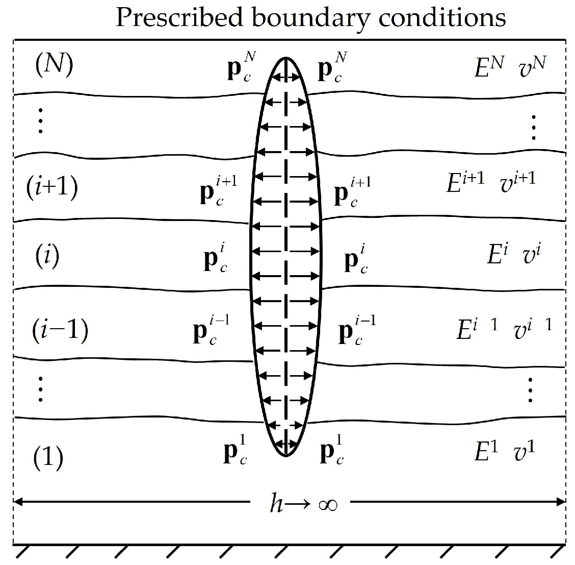
2. Statement of Problem
Figure 1 shows the configuration of the crack problem in the paper. A pressurized crack under known pressure pc passes through a number of layers. Each layer, characterized by Young’s modulus E and Poisson ratio v, is assumed homogeneous and isotropic individually [53]. The objective is to determine the crack opening displacement D in the quasi-static problem. We shall compare the crack opening displacement obtained with a boundary-element method with those obtained with an analytical or semi-analytical solution, if any. The percentage error of the method to be tested is defined as
where Dn is the crack opening obtained with the method to be tested, and Da represents the crack opening determined with the benchmark method.
Err% = 100% × (Dn − Da)/Da
The labeling in the figure follows the convention of the works authored by Maier and Novati [54]. The index (i) denotes the i-th layer and ranges from 1 (the bottom layer) to N (the top layer). The superscript i represents the material properties and quantities of interest (traction and displacement) associated with the i-th layer. The long dash line in the center implies the initial status of a slit-like crack characterized by two surfaces, one of which overlaps the other effectively. The two short dash lines at the two sides indicate the fictitious side boundaries, which are assumed in “undisturbed” regions and characterized by vanishing (zero) displacement, since the distance of them, h, is assumed to be infinite.
Matrices and column vectors are denoted by bold symbols. Thus, vectors of the nodal traction and displacement are indicated by p and u, respectively. The quantities pertaining to the lower (bottom), upper (top), side boundaries, and crack surfaces of each layer are denoted by the subscripts b, t, s, and c, respectively.
The boundary conditions of the multilayered system are usually of the type
where 0 is the null matrix or vector, and p0 indicates the vector of the given nodal tractions on the very top surface of the system. The former of Equation (1) usually reflects an underlying rigid rock formation characterized by zero displacement beneath the bottom of the multilayered media [45,54]. The boundary condition on the side boundaries is then
ub1 = 0, ptN = p0
usi = 0 (1 ≤ i ≤ N)
As a result, the equations associated with the side boundaries can be split out of those pertaining to other boundaries [54].
The local coordinate defined in [41] is adopted in the paper, leading to the following interface continuity conditions (see the Appendix A for details).
uti = −ubi+1, pti = pbi+1
3. Displacement Discontinuity Method (DDM)
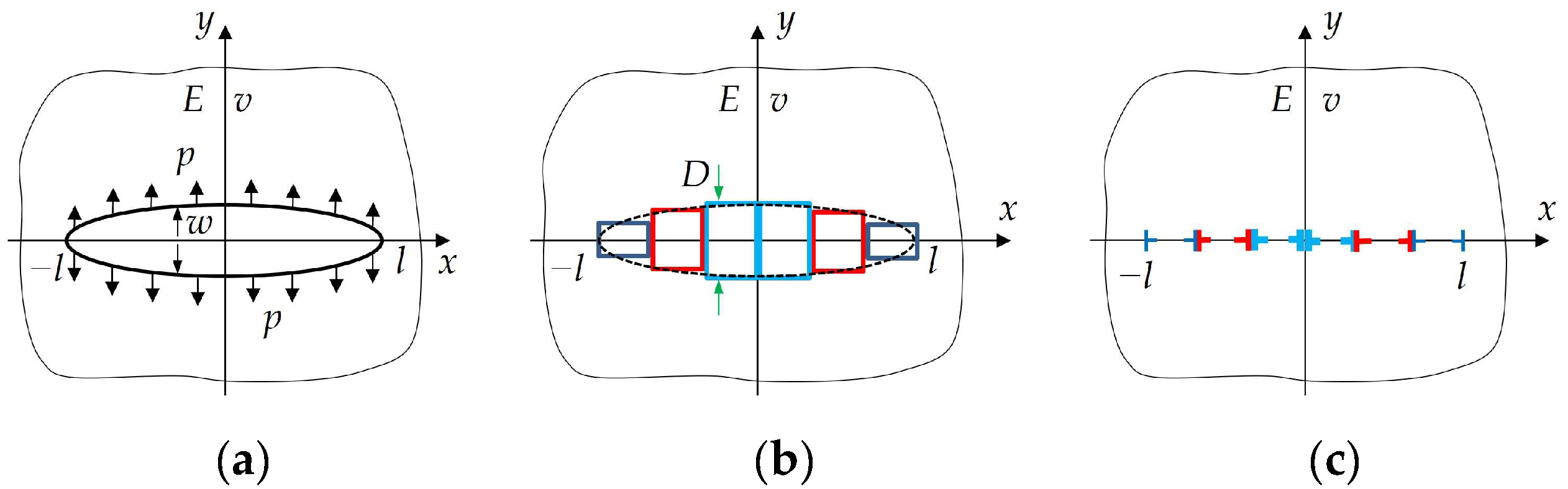
The DDM, proposed by Crouch [49], exploits the physical analog of a slit-like crack and a distribution of a series of constant displacement discontinuities or a distribution of a series of edge-dislocation dipoles (Figure 2). As a result, the DDM only focuses on the elements on the crack surface by discretizing it as a unity. In other words, it is not necessary for the DDM to introduce elements along interfaces, if any, while other numerical methods have to take care of the interfaces, making the DDM perhaps the most efficient numerical method for an analysis of the crack problems [37].
3.1. Homogeneous Medium
The DDM was proposed under the assumption that (1) a crack lies in a homogeneous and isotropic medium and (2) equal loadings apply on the two crack surfaces (Figure 2a). The boundary-element equation of the DDM can be written in a concise form as
where K is the coefficient matrix obtained from the DDM. Its explicit form is referred to in Ref. [49]. It is worth noting that the K obtained from the theory of constant displacement discontinuities and that obtained from the theory of edge dislocation are mathematically the same. D is the nodal opening displacement of the elements on the crack surface. p is the known nodal pressure on the crack surface. Thus, the crack opening displacement is
KD = p
D = (K)−1p
In addition, the analytical solution to the crack problem in a homogeneous medium is given as the following [55,56]:
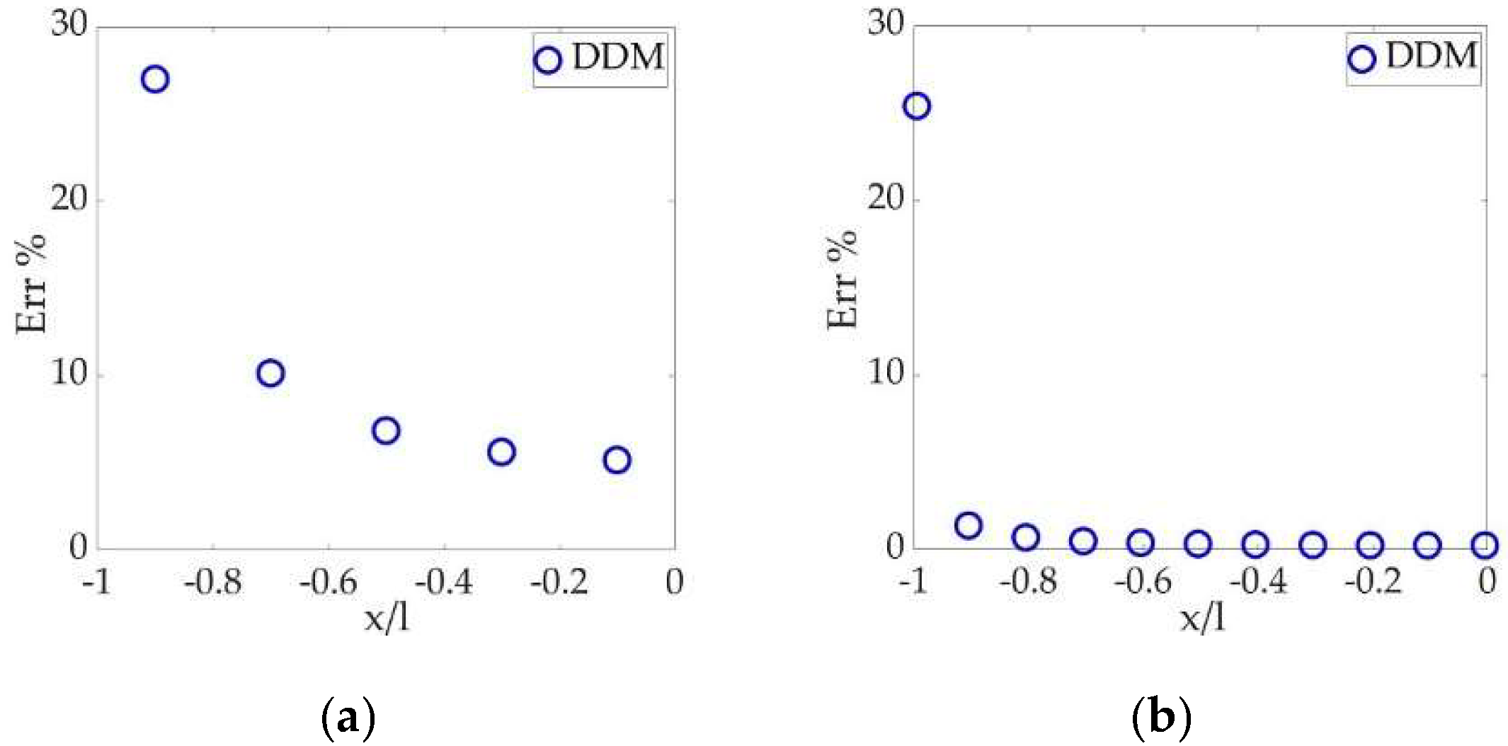
The percentage errors of the DDM with respect to the analytical solution with different numbers of the uniform crack element are illustrated in Figure 3, in which only the left-half part of the crack is displayed because of the symmetry. The abscissa is normalized by x/l, so that the coordinate −1 represents the crack tip. Figure 3b involves 100 crack elements, while only 11 elements are shown for visual simplicity.
Figure 3 demonstrates that a refined mesh leads to a more satisfying accuracy along the crack surface, except the tip, where the error of the DDM keeps around 26%.
3.2. The Higher-Order Tip-Element Approach
In order to improve the tip accuracy of the DDM, Shou and Crouch [57] developed the tip-element approach by replacing the constant displacement discontinuity (DD), also known as the zeroth-order element, at the tips with a higher-order quadratic DD (Figure 4). Constant DD is still assumed for elements other than at the tip, while the higher-order tip element assumes D~r1/2, where D is the opening displacement and r is the distance from a point in the tip element to its nearer tip point (x = −l for the left tip element and x = l for the right tip element). As a result, the approach captures the asymptotic behavior of the near-tip stress field due to the DD, leading to better tip accuracy.
The tip-element approach yields a boundary-element equation in the same form as Equation (4), while the explicit form of the K is referred to in Ref. [57]. The errors of the DDM with the tip element and the conventional DDM are displayed in Figure 5, which demonstrates significant improvement of the tip accuracy due to the higher-order tip element. The tip error decreases from around 26% to around 9%.
The tip-element approach, however, is restricted to the homogeneous medium. Once the media becomes inhomogeneous, the approach fails. In addition, some attempts have been made to place higher-order elements on the whole crack surface for even better accuracy [58,59]. Unfortunately, they are also limited to a homogeneous medium.
3.3. Two Bonded Half-Planes
Although the tip-element approach only applies to the homogeneous medium, the conventional DDM can be extended to the two bonded half-planes (Figure 6), since the Dundur’s equation that characterizes the stress field of an edge dislocation in the two bonded half-planes can be used as an analytical fundamental solution [55,60].
The DDM for the two bonded half-planes results in a boundary-element equation in the same form as Equation (4), while the explicit form of the K is based on the Dundur’s equation and can be referred to Refs. [55,60]. A semi-analytical solution to the crack problem in the two bonded half-planes is available with an additional continuity condition [61,62]:
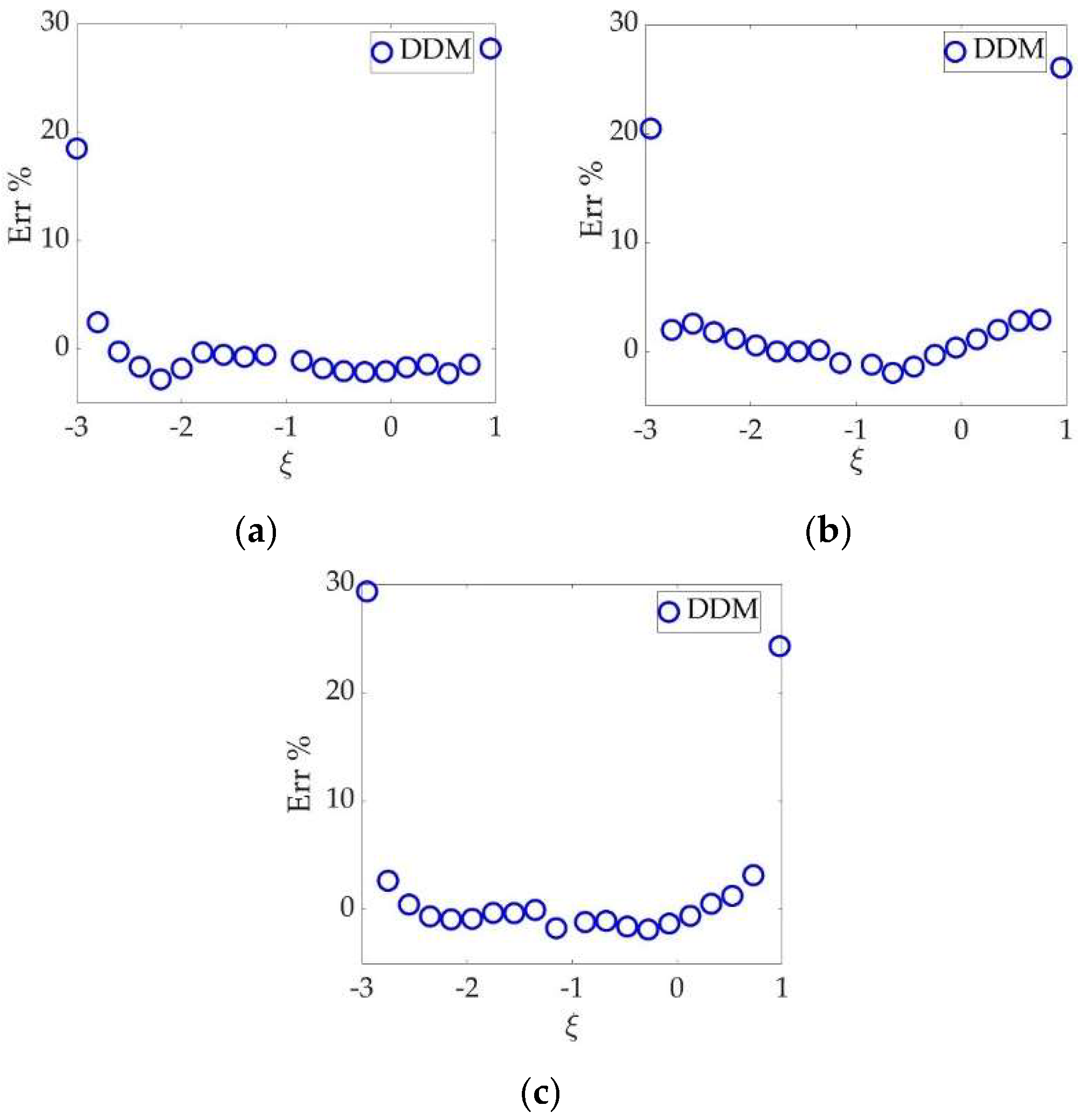
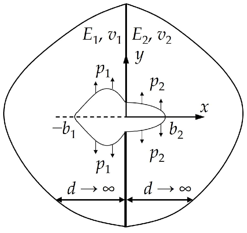
The percentage error of the DDM with respect to the semi-analytical solution is shown in Figure 7. In the computation, the material properties are set as E1 = 3.07 (GPa), v1 = 0.35, E2 = 68.95 (GPa), and v2 = 0.3. The thickness of layer d is assumed to be 100 times of the larger one of b1 and b2, approximating the condition of the infinite d. In total, 10 uniform elements are placed on the shorter segment of the crack for a reasonably refined discretization.
In Figure 7, the abscissa is normalized using
Thus, coordinate −3 and 1 represent the two crack tips. The result shows that the DDM matches well with the benchmark, except at the tip. Unfortunately, we cannot apply the tip-element approach here since the media becomes inhomogeneous.
3.4. Summary
The section has reviewed the DDM and its implementation for the crack problems in a homogeneous medium and two bonded half-planes. The method only requires elements on the crack surface and provides well-accepted accuracy, except at the tip. The tip-element approach improves the tip accuracy significantly, while it is not applicable to inhomogeneous media. In addition, the DDM is restricted in the cases of a homogeneous medium and two bonded half-planes since there are no existing analytical fundamental solutions to construct the boundary-element equations for the DDM in general multilayered media. Although some attempts [20,47,48] have been made to extend the DDM for general multilayered media, the extensions turn out to be first-order approximations, instead of full solutions [63,64]. As a result, we turn to the DM, the other branch of the BEM, for a more applicable implementation.
4. Direct Method (DM)
Unlike the DDM that utilizes a physical analog of a slit-like crack and a distribution of a series of DDs or edge-dislocation dipoles, the traditional boundary-element method determines boundary-element equations directly by using the Kelvin’s solution and the reciprocal theorem [65,66,67,68,69]. Thus, the method is also known as the direct method (DM) [41]. The implementation of the DM for the multilayered media involves construction of a boundary-element equation for each layer and subsequent assembly of the equations with the continuity conditions along interfaces. Such a procedure usually generates an awfully large system of equations, of which all the unknowns are then solved simultaneously, undermining both accuracy and efficiency significantly [70]. Thus, it becomes necessary to decompose the large final system of equations into smaller ones by using the chain-like properties, i.e., the continuity conditions on the interfaces of the multilayered media [53,71]. Unfortunately, the DM cannot distinguish the effects of elements placed along one crack surface from those placed along the other surface. Thus, the DM cannot be applied to the crack problems directly [41]. The implementation of the DM for the multilayered media that does not contain cracks, however, inspires subsequent studies on the DM for the crack problems in multilayered media. As a result, we shall still review the DM here in a relatively concise manner.
4.1. Transfer Stiffness Method (TSM)
Maier and Novati [53] developed a method to decompose the final large system of a boundary-element equation into smaller ones. The method sets up the boundary-element equation for each layer of the multilayered media with the DM in the form
where H is the stiffness matrix obtained from the DM, of which the explicit form is referred to in [41]. It expresses the tractions in terms of the displacements. u and p are the nodal displacement and traction of elements, respectively. The superscript i denotes the current layer (the i-th layer). We can rewrite Equation (9) to (10) by partitioning the boundary elements according to the categorization of the boundaries:
Hiui = pi
When the elements on the top and bottom surfaces are placed in pair (Figure 8a), Equation (10) can be rewritten to Equation (11) so that the quantities on the bottom interface can be expressed in terms of those on the top interfaces after some basic arrangements:
where Tuui = − (Htbi)−1Htti, Tupi = (Htbi)−1, Tpui = Hbti − Hbb(Htbi)−1Htti, and Tppi = Hbbi (Htbi)−1.
Equation (11) can be written into a more concise form as
From Equation (12), we can solve the unknown displacements and tractions on the very top and bottom boundaries of the media using the chain-like property of the multilayered media, i.e., Equation (3), as a continuity condition on the interface:
Equation (13) is a recursive formula. When i = N, we can solve pb1 and utN, since ub1 and ptN are prescribed in Equation (1) as the boundary condition. Having obtained pb1 and utN, we can evaluate i from 2 to N−1 to obtain all the unknown displacements and tractions on the bottom and top interfaces of the layer that ranges from 2 to N−1. In other words, the TSM solves the unknowns by transferring the displacements and tractions on the bottom interface to those on the top interface of a layer with a sequential product of matrices from T1 to Ti.
Although the TSM manages to decompose the large final system of equations into smaller ones to improve efficiency, it suffers several computational issues that limit its application severely [45,54]:
- (1)
- It requires elements on the top and bottom interfaces in pair;
- (2)
- It categorizes the elements according to the type of unknown (displacement or traction). In practical applications, however, the displacement in mm and traction in kPa or MPa differs in magnitude of several orders. Therefore, an extra scaling that makes displacement and traction in the same order is necessary in case of ill-conditioning, undermining the efficiency of the method;
- (3)
- It results in a highly ill-conditioned matrix H when dealing with a thick layer.
In order to address the issues above, Maier and Novati [54] proposed the successive stiffness method (SSM) that can be implemented in a more robust manner.
4.2. Successive Stiffness Method (SSM)
The SSM follows the same path of the TSM until Equation (10), from which the SSM derives a recursive formula [54]:
where Ĥ is the stiffness matrix of the i-th layer. When i = 1,
pti = Ĥttiuti
Ĥtt1 = Htt1
When i = 2~N,
Ĥtti = Htti − Htbi(Hbbi + Ĥtti−1)Hbti
Based on Equation (14), the SSM derived another two recursive formulae for i = 2~N:
ubi = [(Ĥtti−1 − Hbbi)−1Hbti]uti
pbi = Ĥtti−1uti
Having obtained Equations (14), (17) and (18), we can firstly obtain utN from Equation (14), since ptN is given as a boundary condition. Substitution of the solved utN into Equations (17) and (18) with i = N solves both ubN and pbN. The continuity condition on the interface gives utN−1 = −ubN and ptN−1 = pbN. Then, we can repeat the procedure to obtain ubN−1 and pbN−1 by replacing i = N by i = N − 1 in Equations (17) and (18). In such a recursive manner, we can compute all the unknowns successively from the very top layer to the very bottom one in a descending order, making the method quite convenient for numerical implementation. In addition, the method does not suffer the computational issues of the TSM.
4.3. Summary
The section has reviewed the DM and its implementation for multilayered media. The TSM decomposes the final large system of equations by utilizing the chain-like property (continuity condition on interfaces) of the media and categorizing the boundary element according to the type of unknown (displacement or traction). On the other hand, the SSM categorizes the boundary element by the categorization of the boundaries (bottom or top) and consequently overcomes the computational issues of the TSM. It is worth noting that neither the two methods are applicable for the crack problems directly, since the DM cannot distinguish the effects of elements placed along one crack surface from those placed along the other crack surface. The development of the SSM, however, inspires us to conceive a different approach to implement the DM so that it can be used for crack problems in multilayered media.
5. Consecutive Stiffness Method (CSM)
5.1. Pre-Treatment
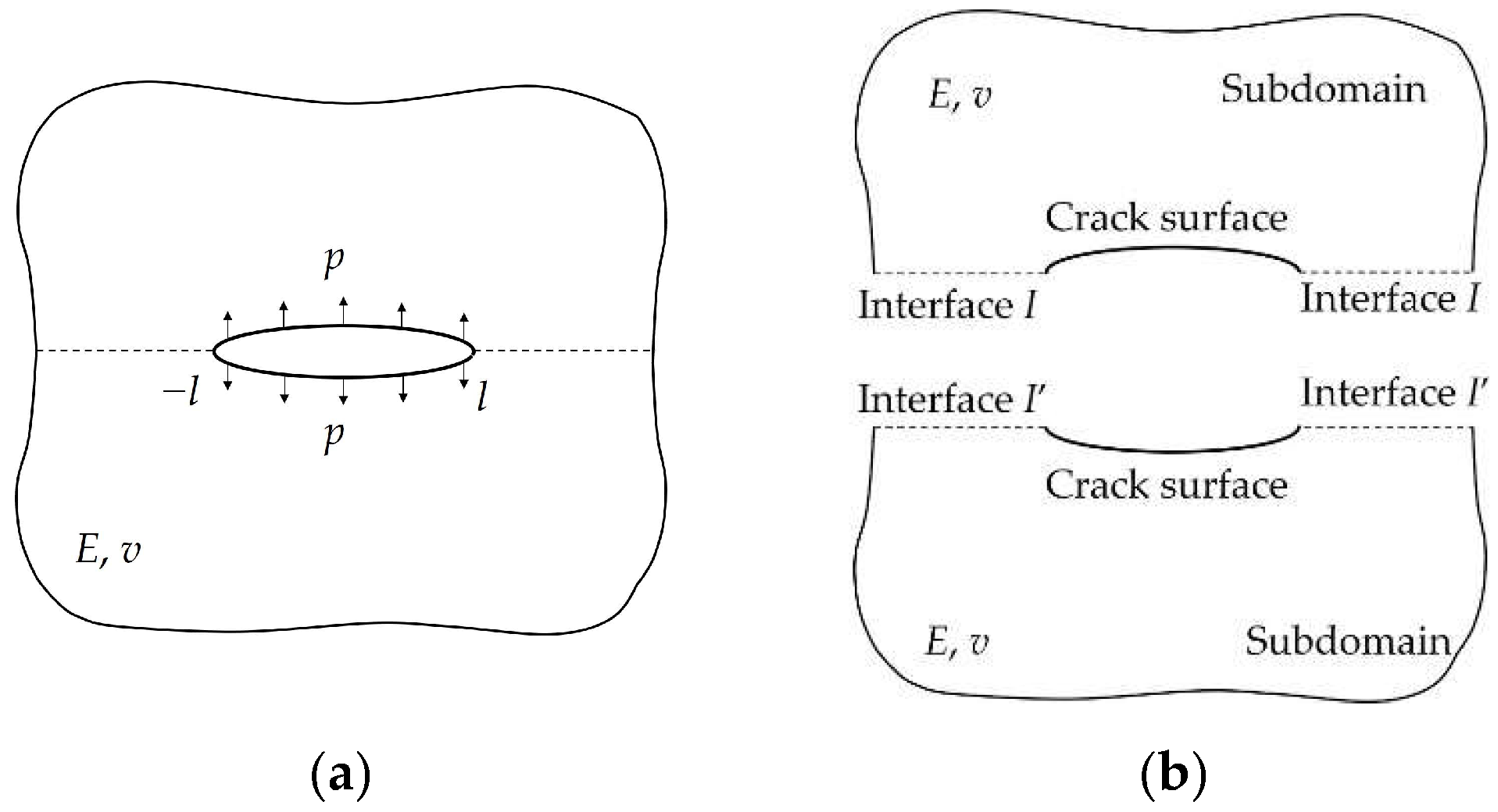
The inapplicability of the DM to solve crack problems is attributed to the incapability of the DM to distinguish effects of the elements on the two overlapping crack surfaces [41]. If we divide the media artificially along the crack surface, however, the media will be divided into two subdomains with a pair of imaginary interfaces denoted by I and I’ (Figure 9). Then, we construct the boundary-element equation for each subdomain and assemble them with the continuity conditions on I and I’. The assembled equation turns out to be applicable to computing opening displacement of a slit-like crack [38,41].
We can now solve the crack problem in a homogeneous medium by dividing the medium in the way shown in Figure 9 and obtain the assembled boundary-element equation to compute the crack opening displacement. The details of the assembly and the consequent discretization can be referred to in Ref. [72]. The results obtained with the DM are compared to those obtained with the conventional DDM and the DDM with the tip element (Figure 10).
Figure 10 indicates that the DM shows the most satisfying accuracy except at the tip, since the integrals involved in the implementation of the DM can be evaluated analytically under the plane–strain condition [41]. Although the higher-order tip-element approach yields the best tip accuracy, the DM that uses the zeroth-order element can still obtain a comparable accuracy at the tip. On the other hand, the requirement of the pre-treatment makes the DM much slower than the DDM (Table 1).
All the computations in the paper were conducted with MATLAB 2021a on a desktop with an Intel(R) Core (TM) i9-13900KF 3.00GHz CPU and 32GB RAM. Table 1 clearly indicates that the DM is much slower than the DDM, not only because of the pre-treatment but also due to the necessity to take care of the elements on the resultant interfaces I and I’, while the DDM only concentrates on the crack surface elements.
The pre-treatment shown in Figure 9 enables the application of the DM for crack problems in multilayered media. In Figure 11, the blue and red lines represent the two crack surfaces that effectively overlap each other, respectively. We cut the media along the crack surface (Figure 11a) artificially and acquire the resultant subdomains (Figure 11b). After that, we set up a boundary-element equation for each subdomain and assembled the equations with continuity conditions on all the interfaces.
It is obvious that an increase in the number of layers leads to a more cumbersome implementation, as we need to set up the boundary-element equation for each subdomain and assemble them all together. The procedure finally results in an extraordinarily huge system of equations, further deteriorating the efficiency of the DM. In order to improve the efficiency, Long et al. [72] proposed a consecutive stiffness method to break the huge system of equations into smaller ones and enable a recursive formula for faster computation by utilizing the chain-like property, i.e., the interfacial continuity condition of the media.
5.2. Formulations and Algorithm
The CSM divides the media and obtains the resultant subdomain in the way shown in Figure 11. After setting up a boundary-element equation for each subdomain, the CSM assembles two subdomains of a given layer through the resultant interface I’ and I’’, if any. If the given layer is an inner layer, e.g., the i-th layer in Figure 11b, the CSM simply patches the two systems of equations into one, since there is no resultant interface for the layer. Such a procedure eventually leads to a new system of equations for each layer, instead of a system of equations for the whole multilayered media. After that, the CSM derives recursive formulae to calculate unknowns for a faster computation by following the procedure of the SSM. In addition, the CSM derives a particular recursive formula that only focuses on the crack opening displacement uc so that all the other unknowns are eliminated during intermediate procedures, ensuring a further faster computation. Considering the limit of the page, we only present the four key equations of the method below. The detailed derivation of the equations is referred to in Ref. [72].
Equation (21) is the particular recursive formula in which i ranges from 2 to N. In Equations (19)–(22), the matrices, such as Ĥ, , H, A, C, etc., and the vectors at the right-hand side, such as pc, , , , etc., are all known. The details of those quantities are available in Ref. [72]. Having obtained the four equations, we can conduct a sequential computation to solve the displacements on the crack surfaces consecutively in each layer in a descending order from the very top layer to the very bottom one. The flowchart of the computation is shown in Figure 12.
The calculated displacement of a crack surface in all the layers uc contains two parts: the displacement of the upper crack surfaces, denoted by uc+, and that of the lower crack surfaces, denoted by uc−. According to the local coordinate used in the work, the crack opening displacement Dc is the following (see the Appendix A for details):
Dc = uc− + uc+
5.3. Numerical Examples
The discretization of the CSM is referred to in Ref. [72]. We compare the crack opening displacements obtained with the DDM and the CSM for the crack problem in two bonded half-planes (Figure 13).
The parameters remain the same as in Section 3.3. The percentage errors of the DDM and the CSM are displayed in Figure 14.
Figure 14 illustrates that both the DDM and the DM match the semi-analytical solution well along the crack surface, except at the tips. The CSM obtains tip errors that are lower than 20%, which is acceptable for practical engineering applications. Furthermore, the CSM leads to generally satisfactory results when the ratio of crack segments falls in the practical range, i.e., the value of b1/b2 falls in one order of magnitude. The durations of the DDM, CSM, and DM with the artificial subdivision are listed in Table 2.
Table 2 indicates that the CSM is faster than the DM. On the other hand, the CSM that needs to take care of the elements on the interfaces is still slower than the DDM that only focuses on the elements on crack surfaces. The difference gets even larger with an increase in the number of elements.
5.4. Summary
The section has reviewed the CSM that implements the DM in a way that an artificial division of the multilayered media is made, enabling sequential computation to solve the displacements on the crack surfaces in each layer consecutively in a descending order from the very top layer to the very bottom one. Figure 10 and Figure 14 illustrate acceptable accuracy of the DM even with the zeroth-order element because analytical evaluation is available for the integrals involved in the DM under the plane–strain condition [41], indicating that the DM-based CSM can be used as a convincing benchmark to test other methods for crack problems in multilayered media. Furthermore, Table 1 and Table 2 have demonstrated the inefficiency of the CSM.
It is also worth noting that the inefficiency excludes the CSM for practical industrial applications, such as hydraulic-fracturing treatment that usually sets up the system of equations to conduct millions of time steps’ computation because of an excessively small time step for numerical stability [73,74,75,76]. For each time step, the newly introduced elements on the imaginary interfaces due to the artificial division result in a larger system of equations to manipulate [77,78,79], severely deteriorating the efficiency. In addition, when multiple cracks are involved, the CSM gets even slower and cumbersome for numerical implementation, since each crack requires an artificial division and consequent additional computation. Therefore, it is natural to conceive a method that shares both the efficiency of the DDM and broad applicability of the DM after the division.
6. Combined Boundary-Element Method
Ref. [19] incorporated the generalized Kelvin’s solution, the fundamental analytical solution of the DM, to the DDM with the Fourier transform, illustrating combination of the two methods from the aspect of basic theory. On the other hand, Ref. [13] attempts to extend the DDM with a “dividing and patch” approach, showing a simpler combination. Inspired by the two works, Long and Xu [80] presented a method that sets up the stiffness matrix of each layer with the DDM and characterizes the effects of the interfaces with the DM. Thus, the method that combines the DDM and the DM shares both the efficiency of the DDM and broad applicability of the DM after the artificial division.
6.1. Formulations and Algorithm
Figure 15 schematically illustrates a given (the i-th) layer after the deformation due to crack opening. The interfaces are sketched parallel for visual simplicity. Then, two artificial half-planes in the same material property marked in green and blue are patched with the layer on its original bottom and top interfaces (vertical dash lines), respectively.
Having patched the two half-planes to the given layer, we apply tractions of the same magnitudes but in the opposite directions of the interfacial tractions. Thus, the interfaces of the two half-planes deform artificial nodal displacement vbi and vti, respectively (Figure 15b). The nodal displacement discontinuities on the two interfaces are
Dbi = ubi + vbi, Dti = uti + vti
In addition, the resultant medium becomes homogeneous, enabling implementation of the tip-element approach for the resultant artificial crack. Thus, we set up the matrix Ki for the elements at the crack tips marked by red circles in Figure 15b with the tip-element approach and construct Ki for the non-tip elements with the conventional DDM:
where the matrix Ki can be partitioned by the categorization of the boundaries:
where the matrices Kcti, etc., are determined with the configuration of the i-th layer. Thus, they can be treated as known quantities.
KiDi = pi
On the other hand, we can also construct the boundary-element equation for the patched half-planes based on the DM:
where the matrices Hbbi and Htti are determined with the configuration of the patched half-planes only. Therefore, they can also be treated as known quantities.
Hbbivbi = pbi, Httivti = pti
Equations (25) and (27) are the starting point of the combined method. The method derives recursive formulae to obtain the final equation system that contains only the crack opening Dc for an even faster computation. Similar to the review of the CSM (Section 5.2), we only present the key equations of the combined method here, considering the limit of the page. The detailed explanation and derivation are referred to in Ref. [80].
When i = 1, the stiffness matrices of the combined method are
where the matrices , etc., are resultant matrices after fundamental calculations of the basic matrices K, etc., and H, etc., in Equations (25) and (27).
When i = 2~N, the stiffness matrices of the combined method are
where the matrices J, M, N, Q, etc., are also resultant matrices after fundamental calculations of the basic matrices K, etc., and H, etc., in Equations (25) and (27). The details of the matrices are referred to in Ref. [80]. Having calculated , , , and from Equation (29), we can obtain the crack opening displacement :
where contains the crack opening displacement of the elements from the bottom layer (i = 1) to the top layer (i = N). From Equations (28) and (29), we can conduct a sequential computation to compute the stiffness matrix of each layer in an ascending order from the bottom layer to the top one. Having obtained the , we can solve the crack opening displacement from Equation (30). The flowchart of the computation is shown in Figure 16.
6.2. Numerical Examples
6.2.1. Two Bonded Half-Planes
The discretization of the combined method is referred to in Ref. [80]. We firstly compare the percentage errors of the DDM, the CSM, and the combined method for the crack problem in the two bonded half-planes in Figure 17, while the parameters remain the same as in Section 3.3. The figure illustrates a satisfying match of the three methods to the semi-analytical solution, except at the tips. The combined method incorporated with the tip-element approach gives the best tip accuracy. Furthermore, it does not affect the results of the combined method significantly when the crack length ratio remains in the practical range (up to 25) in different materials.
In addition, the durations of the three methods are listed in Table 3, which indicates that the combined method improves the efficiency compared to the CSM, although the DDM that does not require elements on interfaces, if any, is still the most efficient.
6.2.2. General Multilayered Media
The second example is calculation of crack opening in general multilayered media, in which the number of layers is more than three. We chose five-layered media, in which a crack intersects the parallel interfaces perpendicularly (Figure 18).
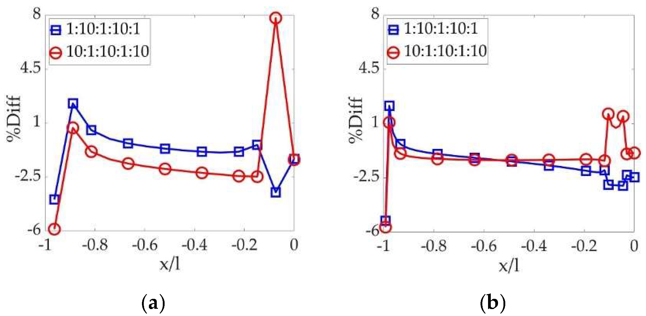
We set the crack segment as l1 = 12l2. The Poisson ratios of the softer and stiffer layers are 0.25 and 0.3, respectively. The pressure p0 remains a known constant. The percentage difference of the crack opening displacement obtained using the combined method and that obtained using the CSM with a different Young’s modulus contrast and different numbers of the crack element on the thin layers are displayed from Figure 19, Figure 20 and Figure 21, in which only half of the results are shown due to the symmetry.
All of the three figures clearly illustrate a “peak” difference on the thin-and-softer layers neighbored by thick-and-stiffer ones. Fortunately, we can alleviate the “peak” difference by refining the discretization. In addition, higher E contrast results in a higher “peak” difference and requires more refined elements to mitigate it consequently. When the discretization is refined sufficiently, the results obtained with the two methods are quite close to each other.
6.2.3. Approximation of Thin-Layer Scaling
In practical hydraulic-fracturing treatments, a fluid-driven crack sometimes passes through a few thin layers sandwiched by thicker ones. Such thin layers usually require awfully refined discretization for accurate simulation, slowing down the computation significantly. It is well accepted that efficiency and accuracy are both critical factors for practical industrial applications. A satisfying numerical simulation in industry should keep a balance between the two factors, instead of sacrificing one to satisfy the other. Thus, the thin layers might be scaled as a single relatively thick layer with average effective material properties as in Equation (31) for better efficiency with the combined method:
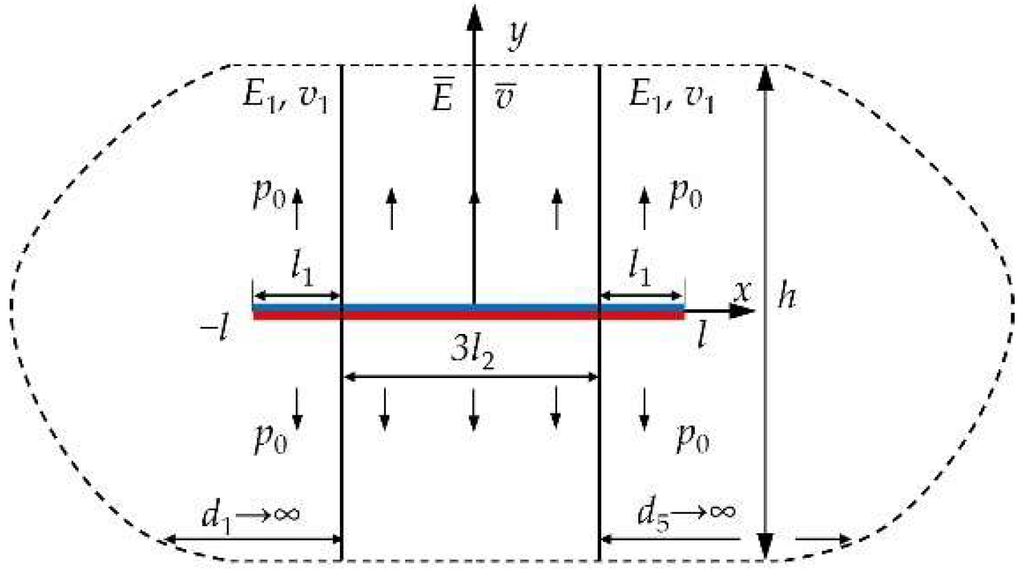
where j is the index of the n thin layers, and lj is the thickness of the j-th layer. Thus, the original crack problem in Figure 18 is approximated with that in Figure 22.
The combined method placed only one crack element on the crack surface in the scaled layer characterized by Ē and v for even faster computation. The calculated crack opening displacement is then compared to that obtained using the combined method with coarse mesh (one element on the thin layer) in the original five-layered media and that obtained using the CSM with refined mesh (five elements on the thin layer) in the original five-layered media. As indicated previously, the results obtained using the CSM with refined mesh can be used as convincing benchmarks. The comparisons with different contrasts in Young’s modulus are shown from Figure 23, Figure 24 and Figure 25. In the three figures, the crack opening displacement w0 is normalized using
where w is the crack opening displacement and G1 is the shear modulus of the first layer.
The three figures validate the approximation of the thin-layer scaling for more efficient computation when the contrast in Young’s modulus remains up to 10-fold, since the approximated crack opening obtained using the combined method differs from the original crack opening obtained using the CSM with refined mesh by less than 20% (Figure 23).
When the contrast in Young’s modulus gets higher, the original crack opening obtained using the CSM with refined mesh on the thin-and-soft layers neighbored by a thick-and-hard one reaches about twice of the approximated opening calculated using the combined method (Figure 24b and Figure 25b). On the other hand, it is interesting to find the approximation to be valid for a contrast in Young’s modulus up to 50-fold when a thin-and-stiff layer is neighbored by thick-and-soft ones (Figure 24a and Figure 25a).
6.3. Summary
The section has reviewed the combined method that constructs the stiffness matrix of each layer with the DDM and characterizes the effects of the interfaces with the DM. As a result, the method shares both the efficiency of the DDM and broad applicability of the DM after the division, as demonstrated in the numerical examples. In addition, the final system of equations only contains unknown crack opening displacements, leading to even faster computation. The combined method has also adopted the tip-element approach, ensuring a well-acceptable accuracy including at the tips, while the tip accuracy cannot be improved with refined discretization only. The numerical examples also validated an approximation of thin-layer scaling with the combined method under practical conditions for a more-efficient industrial simulation, for example, hydraulic-fracturing simulation. The crack intersects interface(s), if any, perpendicularly in the numerical examples, since some analytical or semi-analytical solutions are available in such conditions. In fact, the combined method can deal with more-complicated crack patterns, such as crack inclining to interfaces. Examples of using the method to simulate propagation of practical hydraulic fractures can be found in Refs. [12,51,78].
7. Summary and Outlook
The BEM is widely chosen for an accurate and efficient analysis of crack problems in multilayered media. The two branches of the BEM, the DDM, and the DM have demonstrated their strengths in efficiency and applicability, respectively. Although several attempts have been made to extend the DDM for general multilayered media and various approaches have been developed to accelerate computation conducted with the DM, the numerical examples have still revealed the weaknesses of the DDM and the DM in applicability and efficiency, respectively. Therefore, the review highlighted the combined method that constructs the stiffness matrix of each layer with the DDM and characterizes the effects of the interfaces with the DM so that it shares both the satisfying efficiency of the DDM and the broad applicability of the DM after the artificial division. In addition, the final system of equations of the combined method only contains unknown crack opening displacements, resulting in even faster computation. The tip-element approach was incorporated into the combined method, ensuring satisfactory accuracy including at the tips, while the tip accuracy can hardly be improved with refined discretization only. The numerical examples also validated an approximation of thin-layer scaling with the combined method to further improve the efficiency for practical industrial applications.
The BEM, however, is still limited currently, given challenges to solve crack problems accurately and efficiently in multilayered elastic media associated with more complicated conditions. As a result, pressing needs still exist for future study to explore the area more comprehensively.
- The DDM is an ideal method for crack problems due to its high efficiency. The limited applicability, however, restricts its application severely. The attempts to extend it for general multilayered media by exploiting the method of images with a superposition scheme turn out to be first-order approximates. As a result, new approaches are encouraged for a full solution to extend the DDM.
- Initiation and propagation of a fatigue crack make notable contribution to failure in industry. Computation of such phenomena in multilayered material continues posing challenges for modeling and simulation. In addition, it gets even more complicated when material becomes brittle or quasi-brittle. As a result, it may be interesting to address such issues with the BEM.
- It is getting popular to implement the PFM with the FEM for the analysis of complicated crack patterns in the latest decade. The former derives partial differential governing equations, which are then solved with the latter numerically. On the other hand, few studies have been conducted to incorporate the PFM into the BEM. Thus, it will be quite encouraging to combine the PFM with the BEM for a more efficient and more accurate analysis of more complex crack problems in multilayered media.
Author Contributions
Conceptualization, G.L. and G.X.; methodology, L.L. and G.L.; validation, L.L. and J.Z.; formal analysis, J.Z. and W.X.; writing—original draft preparation, L.L. and G.L.; editing, G.X. and B.X.; supervision, G.L. and G.X.; project administration, G.L. and B.X.; funding acquisition, G.L. and B.X. All authors have read and agreed to the published version of the manuscript.
Funding
This work is supported by the National Natural Science Foundation of China (No. 52004183).
Data Availability Statement
Not applicable.
Acknowledgments
The authors appreciate FrackOptima Inc., Shell International Exploration and Production Inc., and ConocoPhillips for technical supports.
Conflicts of Interest
The authors declare no conflict of interest.
Appendix A
The local coordinate in our study follows the convention that the normal direction points outwards from the surface of the domain of interest and that the shear direction obeys the right-hand rule with respect to the normal one (Figure A1a).
Figure A1a shows displacements and tractions on a pair of interface Elements (1) and (2). We set |u1| = |u2|= u0 and|p1| = |p2|= p0, where u0 and p0 are the magnitudes of the displacement and traction, respectively. According to the interface continuity, we have u1 = u2 = u0 and p1 = −p2 = −p0 under the global coordinate (x, y). The local coordinates of Elements (1) and (2), denoted by (x1, y1) and (x2, y2), respectively, are constructed as illustrated in Figure A1a based on the convention explained above. As a result, u1 = −u0 and p1 = p0 for Element (1), and u2 = u0 and p2 = p0 for Element (2). Therefore, the interface continuity under the local coordinate is
u1 = −u2, p1 = p2
Figure A1.
The local coordinate for (a) interface elements and (b) calculation of opening displacement [41].
Figure A1.
The local coordinate for (a) interface elements and (b) calculation of opening displacement [41].

Figure A1b illustrates displacements of a pair of crack surface elements, denoted by u+ and u− for the upper element and lower element, respectively, due to the loading p. The local coordinates of the two elements are constructed based on the convention. Thus, u+ = −|u + |, and u− = −|u−|. The opening displacement D is defined as the relative displacement of the lower element with respect to the upper one [41]. Thus,
D = −|u−| − |u+| = u− + u+
Equations (A1) and (A2) correspond to Equations (4) and (23), respectively.
The appendix only presents the essence of the local coordinate, the details of which can be found in Ref. [41].
References
- Xiao, H.; Yue, Z. Elastic fields in two joined transversely isotropic media of infinite extent as a result of rectangular loading. Int. J. Numer. Anal. Methods Geomech. 2013, 37, 247–277. [Google Scholar] [CrossRef]
- Xie, Y.; Xiao, H.; Yue, Z. The behavior of vertically non-homogeneous elastic solids under internal rectangular loads. Eur. J. Environ. Civ. Eng. 2022, 26, 1936–1961. [Google Scholar] [CrossRef]
- Xiao, B.; Fang, J.; Long, G.; Tao, Y.; Huang, Z. Analysis of thermal conductivity of damaged tree-like bifurcation network withfractal roughened surfaces. Fractals 2022, 30, 2250104. [Google Scholar] [CrossRef]
- Zhang, Y.; Xiao, B.; Tu, B.; Zhang, G.; Wang, Y.; Long, G. Fractal analysis for thermal conductivity of dual porous media embedded with asymmetric tree-like bifurcation networks. Fractals 2023, 31, 2350046. [Google Scholar] [CrossRef]
- Hamzah, K.; Long, N.; Senu, N.; Eshkuvatov, K. Numerical solution for crack phenomenon in dissimilar materials under various mechanical loadings. Symmetry 2021, 13, 235. [Google Scholar] [CrossRef]
- Liang, M.; Liu, Y.; Xiao, B.; Yang, S.; Wang, Z. An analytical model for the transverse permeability of gas diffusion layer with electrical double layer effects in proton exchange membrane fuel cells. Int. J. Hydrogen Energy 2018, 43, 17880–17888. [Google Scholar] [CrossRef]
- Xiao, B.; Huang, Q.; Chen, H.; Chen, X.; Long, G. A fractal model for capillary flow through a single tortuous capillary with roughened surfaces in fibrous porous media. Fractals 2021, 29, 2150017. [Google Scholar] [CrossRef]
- An, S.; Zou, H.; Li, W.; Deng, Z. Experimental investigation on the vibration attenuation of tensegrity prisms integrated with particle dampers. Acta Mech. Solida Sin. 2022, 35, 672–681. [Google Scholar] [CrossRef]
- Gao, J.; Xiao, B.; Tu, B.; Chen, F.; Liu, Y. A fractal model for gas diffusion in dry and wet fibrous media with tortuous converging-diverging capillary bundle. Fractals 2022, 30, 2250176. [Google Scholar] [CrossRef]
- Liu, S.; Valko, P.; McKetta, S.; Liu, X. Microseismic closure window characterizes hydraulic-fracture geometry better. SPE Reserv. Eval. Eng. 2017, 20, 423–445. [Google Scholar] [CrossRef]
- Adachi, J.; Siebrits, E.; Peirce, A.; Desroches, J. Computer simulation of hydraulic fractures. Int. J. Rock Mech. Min. Sci. 2007, 44, 739–757. [Google Scholar] [CrossRef]
- Long, G.; Liu, S.; Xu, G.; Wong, S.; Chen, H.; Xiao, B. A perforation-erosion model for hydraulic-fracturing applications. SPE Prod. Oper. 2018, 33, 770–783. [Google Scholar] [CrossRef]
- Shen, B.; Stephansson, O.; Rinne, M. Modelling Rock Fracturing Processes: A Fracture Mechanics Approach Using FRACOD; Springer: London, UK, 2014. [Google Scholar]
- Cui, C.; Zhang, Q.; Banerjee, U.; Babuška, I. Stable generalized finite element method (SGFEM) for three-dimensional crack problems. Numer. Math. 2022, 152, 475–509. [Google Scholar] [CrossRef]
- Liu, S.; Valko, P. A rigorous hydraulic-fracture equilibrium-height model for multilayer formations. SPE Prod. Oper. 2018, 33, 214–234. [Google Scholar] [CrossRef]
- Xiao, B.; Zhu, H.; Chen, F.; Long, G.; Li, Y. A fractal analytical model for Kozeny-Carman constant and permeability of roughened porous media composed of particles and converging-diverging capillaries. Powder Technol. 2023, 420, 118256. [Google Scholar] [CrossRef]
- Cheng, W.; Jiang, G.; Xie, J.; Wei, Z.; Zhou, Z.; Li, X. A simulation study comparing the Texas two-step and the multistage consecutive fracturing method. Pet. Sci. 2019, 16, 1121–1133. [Google Scholar] [CrossRef]
- Xiao, H.; Yue, Z.; Zhao, X. A generalized Kelvin solution based method for analyzing elastic fields in heterogeneous rocks due to reservoir water impoundment. Comput. Geosci. 2012, 43, 126–136. [Google Scholar] [CrossRef]
- Xiao, H.; Yue, Z. A three-dimensional displacement discontinuity method for crack problems in layered rocks. Int. J. Rock Mech. Min. Sci. 2011, 48, 412–420. [Google Scholar] [CrossRef]
- Hirose, S.; Sharma, M. Numerical Modelling of Fractures in Multilayered Rock Formations Using a Displacement Discontinuity Method. In In Proceedings of the 52nd U.S. Rock Mechanics/Geomechanics Symposium, Seattle, WA, USA, 17–20 June 2018. [Google Scholar]
- Zeng, Q.; Bo, L.; Liu, W.; Huang, Z.; Yao, J. An investigation of hydraulic fracture propagation in multi-layered formation via the phase field method. Comput. Geotech. 2023, 156, 105258. [Google Scholar] [CrossRef]
- Zhu, D.; Zhang, L.; Song, X.; Lian, H.; Niu, D. Propagation mechanism of the hydraulic fracture in layered-fractured-plastic formations. Int. J. Fract. 2023, 241, 189–210. [Google Scholar] [CrossRef]
- Xiao, B.; Wang, P.; Wu, J.; Zhu, H.; Liu, M.; Liu, Y.; Long, G. A novel fractal model for gas diffusion coefficient in dry porous media embedded with a damaged tree-like branching network. Fractals 2022, 30, 2250150. [Google Scholar] [CrossRef]
- Alizadeh, R.; Marji, M.; Abdollahipour, A.; Sagand, M. Numerical simulation of fatigue crack propagation in heterogeneous geomaterials under varied loads using displacement discontinuity method. J. Rock Mech. Geotech. Eng. 2023, 15, 702–716. [Google Scholar] [CrossRef]
- Zhuang, X.; Li, X.; Zhou, S. Transverse penny-shaped hydraulic fracture propagation in naturally-layered rocks under stress boundaries: A 3D phase field modeling. Comput. Geotech. 2023, 155, 105205. [Google Scholar] [CrossRef]
- Zhang, G.; Guo, T.; Elkhodary, K.; Tang, S.; Guo, X. Mixed Graph-FEM phase field modeling of fracture in plates and shells with nonlinearly elastic solids. Comput. Methods Appl. Mech. Eng. 2022, 389, 114282. [Google Scholar] [CrossRef]
- Li, P.; Li, W.; Li, B.; Yang, S.; Shen, Y.; Wang, Q.; Zhou, K. A review on phase field models for fracture and fatigue. Eng. Fract. Mech. 2023, 289, 109419. [Google Scholar] [CrossRef]
- Zhang, G.; Qiu, H.; Elkhodary, K.; Tang, S.; Peng, D. Modeling tunable fracture in hydrogel shell structures for biomedical applications. Gels 2022, 8, 515. [Google Scholar] [CrossRef] [PubMed]
- Chen, L. Phase-Field Modelling of Material Microstructure. Multiscale Materials Modelling Fundamentals and Applications; Woodhead Publishing: Sawston, UK, 2007; pp. 62–83. [Google Scholar]
- Zhang, G.; Guo, T.; Guo, X.; Tang, S.; Flemming, M.; Liu, W. Fracture in tension-compression-asymmetry solids via phase field modeling. Comput. Methods Appl. Mech. Eng. 2019, 357, 112573. [Google Scholar] [CrossRef]
- Zhang, G.; Tang, C.; Chen, P.; Long, G.; Cao, J.; Tang, S. Advancements in phase-field modeling for fracture in nonlinear elastic solids under finite deformations. Mathematics 2023, 11, 3366. [Google Scholar] [CrossRef]
- Zhang, Q.; Cui, C.; Banerjee, U.; Babuška, I. A condensed generalized finite element method (CGFEM) for interface problems. Comput. Methods Appl. Mech. Eng. 2022, 391, 114537. [Google Scholar] [CrossRef]
- Ambati, M.; Gerasimov, T.; De Lorenzis, L. A review on phase-field models of brittle fracture and a new fast hybrid formulation. Comput. Mech. 2015, 55, 383–405. [Google Scholar] [CrossRef]
- Cheng, W.; Jin, Y.; Chen, M.; Jiang, G. Numerical stress analysis for the multi-casing structure inside a wellbore in the formation using the boundary element method. Pet. Sci. 2017, 14, 126–137. [Google Scholar] [CrossRef]
- Wang, P.; Xiao, B.; Gao, J.; Zhu, H.; Liu, M.; Long, G.; Li, P. A novel fractal model for spontaneous imbibition in damaged tree-like branching networks. Fractals 2023, 31, 2350010. [Google Scholar] [CrossRef]
- Cheng, W.; Lu, C.; Feng, G.; Xiao, B. Ball sealer tracking and seating of temporary plugging fracturing technology in the perforated casing of a horizontal well. Energy Explor. Exploit. 2021, 39, 2045–2061. [Google Scholar] [CrossRef]
- Peirce, A.; Siebrits, E. Uniform asymptotic approximations for accurate modeling of cracks in layered elastic media. Int. J. Fract. 2001, 110, 205–239. [Google Scholar] [CrossRef]
- Blandford, G.; Ingraffea, A.; Liggett, J. Two-dimensional stress intensity factor computations using the boundary element method. Int. J. Numer. Methods Eng. 1981, 17, 387–404. [Google Scholar] [CrossRef]
- Detournay, E.; Gordeliy, E. Displacement discontinuity method for modeling axisymmetric cracks in an elastic half-space. Int. J. Solids Struct. 2011, 48, 2614–2629. [Google Scholar]
- Yue, Z.; Xiao, H. Generalized Kelvin solution based boundary element method for crack problems in multilayered solids. Eng. Anal. Bound. Elem. 2002, 26, 691–705. [Google Scholar] [CrossRef]
- Crouch, S.; Starfield, A. Boundary Element Methods in Solid Mechanics; George Allen & Unwein: London, UK, 1983. [Google Scholar]
- Thompson, W. Transmission of elastic waves through a stratified medium. J. Appl. Phys. 1950, 21, 89–93. [Google Scholar] [CrossRef]
- Gilbert, F.; Backus, G. Propagator matrices in elastic wave and vibration problems. Geophysics 1966, 31, 326–332. [Google Scholar] [CrossRef]
- Buffler, H. Theory of elasticity of a multilayered medium. J. Elast. 1971, 1, 125–143. [Google Scholar] [CrossRef]
- Peirce, A.; Siebrits, E. The scaled flexibility matrix method for the efficient solution of boundary value problems in 2D and 3D layered elastic media. Comput. Methods Appl. Mech. Eng. 2001, 190, 5935–5956. [Google Scholar] [CrossRef]
- Benitez, F.; Rosakis, A. Three-dimensional elastostatics of a layer and a layered medium. J. Elast. 1987, 18, 3–50. [Google Scholar] [CrossRef]
- Shou, K.; Napier, J. A two-dimensional linear variation displacement discontinuity method for three-layered elastic media. Int. J. Rock Mech. Min. Sci. 1999, 36, 719–729. [Google Scholar] [CrossRef]
- Shou, K. A superposition scheme to obtain fundamental boundary element solutions in multi-layered elastic media. Int. J. Numer. Anal. Methods Geomech. 2000, 24, 795–814. [Google Scholar] [CrossRef]
- Crouch, S. Solution of plane elasticity problems by the displacement discontinuity method. Int. J. Numer. Methods Eng. 1976, 10, 301–343. [Google Scholar] [CrossRef]
- Cheng, W.; Lu, C.; Xiao, B. Perforation optimization of intensive-stage fracturing in a horizontal well using a coupled 3D-DDM fracture model. Energies 2021, 14, 2393. [Google Scholar] [CrossRef]
- Long, G.; Xu, G. The effects of perforation erosion on practical hydraulic-fracturing applications. SPE J. 2017, 22, 645–659. [Google Scholar] [CrossRef]
- Cheng, W.; Lu, C.; Zhou, Z. Modeling of borehole hydraulic fracture initiation and propagation with pre-existing cracks using the displacement discontinuity method. Geotech. Geol. Eng. 2020, 38, 2903–2912. [Google Scholar] [CrossRef]
- Maier, G.; Novati, G. On boundary element-transfer matrix analysis of layered elastic systems. Eng. Anal. 1986, 3, 208–216. [Google Scholar] [CrossRef]
- Maier, G.; Novati, G. Boundary element elastic analysis of layered soils by a successive stiffness method. Int. J. Numer. Anal. Methods Geomech. 1987, 11, 435–447. [Google Scholar] [CrossRef]
- Asaro, R.; Lubarda, V. Mechanics of Solids and Materials; Cambridge University Press: New York, NY, USA, 2006. [Google Scholar]
- Yan, X. An effective boundary element method for analysis of crack problems in a plane elastic plate. Appl. Math. Mech. 2005, 26, 814–822. [Google Scholar]
- Shou, K.; Crouch, S. A higher order displacement discontinuity method for analysis of crack problems. Int. J. Rock Mech. Min. Sci. Geomech. Abstr. 1995, 32, 49–55. [Google Scholar] [CrossRef]
- Shou, K.; Siebrits, E.; Crouch, S. A higher-order displacement discontinuity method for three-dimensional elastostatic problems. Int. J. Rock Mech. Min. Sci. 1997, 34, 317–322. [Google Scholar] [CrossRef]
- Li, J.; Liu, Y.; Wu, K. A new higher-order displacement discontinuity method based on the joint element for analysis of close-spacing planar fractures. SPE J. 2022, 27, 1123–1139. [Google Scholar] [CrossRef]
- Dundurs, J. Elastic Interactions of Dislocations with Inhomogeneities; ASME: New York, NY, USA, 1969; pp. 70–115. [Google Scholar]
- Erdogan, F.; Biricikoglu, V. Two bonded half planes with a crack going through the interface. Int. J. Eng. Sci. 1973, 11, 745–766. [Google Scholar] [CrossRef]
- Cook, L.; Erdogan, F. Stresses in bonded materials with a crack perpendicular to the interface. Int. J. Eng. Sci. 1972, 10, 677–697. [Google Scholar] [CrossRef]
- Siebrits, E.; Crouch, S. On the paper “A two-dimensional linear variation displacement discontinuity method for three-layered elastic media” by Keh-Jian Shou and J.A.L. Napier, International Journal of Rock Mechanics and Mining Sciences, Vol. 36(6), 719-729, 1999. Int. J. Rock Mech. Min. Sci. 2000, 37, 873–875. [Google Scholar] [CrossRef]
- Shou, K.; Napier, J. Author’s reply to discussion by E. Siebrits and S. L. Crouch regarding the paper ‘A two-dimensional linear variation displacement discontinuity method for three-layered elastic media’, Keh-Jian Shou and J.A.L. Napier, International Journal of Rock Mechanics and Mining Sciences, Vol. 36(6), 719–729, 1999. Int. J. Rock Mech. Min. Sci. 2000, 37, 877–878. [Google Scholar]
- Nowak, P.; Hall, J. Direct boundary element method for dynamics in a half-space. Bull. Seismol. Soc. Am. 1993, 83, 1373–1390. [Google Scholar] [CrossRef]
- Segond, D.; Tafreshi, A. Stress analysis of three-dimensional contact problems using the boundary element method. Eng. Anal. Bound. Elem. 1998, 22, 199–214. [Google Scholar] [CrossRef]
- Tsinopoulos, S.; Kattis, S.; Polyzos, D.; Beskos, D. An advanced boundary element method for axisymmetric elastodynamic analysis. Comput. Methods Appl. Mech. Eng. 1999, 175, 53–70. [Google Scholar] [CrossRef]
- Oliveria, M.; Dumont, N.; Selvadurai, A. Boundary element formulation of axisymmetric problems for an elastic halfspace. Eng. Anal. Bound. Elem. 2012, 36, 1478–1492. [Google Scholar] [CrossRef]
- Hattori, G.; Alatawi, I.; Trevelyan, J. An extended boundary element method for formulation for the direct calculation of the stress intensity factors in fully anisotropic materials. Int. J. Numer. Anal. Methods Geomech. 2017, 109, 965–981. [Google Scholar] [CrossRef]
- Linkov, A.; Fillipov, N. Difference equations approach to the analysis of layered systems. Meccanica 1991, 26, 195–209. [Google Scholar] [CrossRef]
- Siebrits, E.; Peirce, A. An efficient multi-layer planar 3D fracture growth algorithm using a fixed mesh approach. Int. J. Numer. Methods Eng. 2002, 53, 691–717. [Google Scholar] [CrossRef]
- Long, G.; Liu, Y.; Xu, W.; Zhou, P.; Zhou, J.; Xu, G.; Xiao, B. Analysis of crack problems in multilayered elastic medium by a consecutive stiffness method. Mathematics 2022, 10, 4403. [Google Scholar] [CrossRef]
- Cheng, W.; Jiang, G.; Zhou, Z.; Wei, Z.; Li, X. Numerical simulation for the dynamic breakout of a borehole using boundary element method. Geotech. Geol. Eng. 2019, 38, 2873–2881. [Google Scholar] [CrossRef]
- Al Hameli, F.; Suboyin, A.; Al Kobaisi, M.; Rahman, M.; Haroun, M. Modeling fracture propagation in a dual-porosity system: Pseudo-3D-carter-dual-porosity model. Energies 2022, 15, 6779. [Google Scholar] [CrossRef]
- Donstov, E. Analysis of a constant height hydraulic fracture driven by a power-law fluid. Rock Mech. Bull. 2022, 1, 100003. [Google Scholar]
- Luo, T.; Liu, S.; Liu, S. A productivity model for vertical wells with horizontal multi-fractures. Int. J. Oil Gas Coal Technol. 2022, 31, 225–241. [Google Scholar] [CrossRef]
- Cheng, H.; Detournay, A. A direct boundary element method for plane strain poroelasticity. Int. J. Numer. Anal. Methods Geomech. 1988, 12, 551–572. [Google Scholar] [CrossRef]
- Zhai, Z.; Fonseca, E.; Azad, A.; Cox, B. A new tool for multi-cluster & multi-well hydraulic fracture modeling. In Proceedings of the SPE Hydraulic Fracturing Technology Conference, Woodlands, TX, USA, 3–5 February 2015. [Google Scholar]
- Munoz, L.; Mejia, C.; Rueda, J.; Roehl, D. Pseudo-coupled hydraulic fracturing analysis with displacement discontinuity and finite element methods. Eng. Fract. Mech. 2022, 274, 108774. [Google Scholar] [CrossRef]
- Long, G.; Xu, G. A combined boundary integral method for analysis of crack problems in multilayered elastic media. Int. J. Appl. Mech. 2016, 8, 1650070. [Google Scholar] [CrossRef]
Figure 1.
Schematic view of the crack problem [54].
Figure 1.
Schematic view of the crack problem [54].

Figure 2.
Physical analog of (a) a slit-like crack and (b) a distribution of a series of constant displacement discontinuities or (c) a distribution of a series of edge-dislocation dipoles.
Figure 2.
Physical analog of (a) a slit-like crack and (b) a distribution of a series of constant displacement discontinuities or (c) a distribution of a series of edge-dislocation dipoles.

Figure 3.
Percentage errors of the DDM with (a) 5 elements and (b) 100 elements.

Figure 4.
The DDM (a) without the tip-element approach and (b) with the tip-element approach.

Figure 5.
Percentage errors of the conventional DDM and the DDM with the tip element: (a) 5 crack elements and (b) 100 crack elements.
Figure 5.
Percentage errors of the conventional DDM and the DDM with the tip element: (a) 5 crack elements and (b) 100 crack elements.

Figure 6.
Physical analog of (a) a slit-like crack in two bonded half-planes and (b) a distribution of a series of edge-dislocation dipoles.
Figure 6.
Physical analog of (a) a slit-like crack in two bonded half-planes and (b) a distribution of a series of edge-dislocation dipoles.

Figure 7.
Percentage error of the DDM with b1/b2 = (a) 1/25; (b) 1/1; and (c) 2/1.

Figure 8.
Elements on the top and bottom interfaces are placed (a) in pair and (b) not in pair.

Figure 9.
The artificial division: (a) division of the original media along the crack surface (dash line) and (b) the resultant subdomains and the imaginary interfaces I and I’.
Figure 9.
The artificial division: (a) division of the original media along the crack surface (dash line) and (b) the resultant subdomains and the imaginary interfaces I and I’.

Figure 10.
Percentage errors of the conventional DDM, the DM, and the DDM with tip element: (a) 5 crack elements and (b) 100 crack elements.
Figure 10.
Percentage errors of the conventional DDM, the DM, and the DDM with tip element: (a) 5 crack elements and (b) 100 crack elements.

Figure 11.
Pre-treatment of the DM for crack problems in multilayered media: (a) original configuration and (b) resultant configuration after the division.
Figure 11.
Pre-treatment of the DM for crack problems in multilayered media: (a) original configuration and (b) resultant configuration after the division.

Figure 12.
Flowchart of the computation to solve crack problems in multilayered media with the CSM.

Figure 13.
Schematic view of the crack problem in two bonded half-planes.

Figure 14.
Percentage errors of the DDM and the CSM with b1/b2 = (a) 1/25; (b) 1/1; and (c) 2/1.

Figure 15.
Schematic view of the artificial patch: (a) the i-th layer after the deformation and (b) the i-th layer patched with two half-planes in the same material property.
Figure 15.
Schematic view of the artificial patch: (a) the i-th layer after the deformation and (b) the i-th layer patched with two half-planes in the same material property.

Figure 16.
Flowchart of the computation to solve crack problems in multilayered media with the combined method.
Figure 16.
Flowchart of the computation to solve crack problems in multilayered media with the combined method.

Figure 17.
Percentage errors of the DDM, the CSM, and the combined method with b1/b2 = (a) 1/25; (b) 1/1; and (c) 2/1.
Figure 17.
Percentage errors of the DDM, the CSM, and the combined method with b1/b2 = (a) 1/25; (b) 1/1; and (c) 2/1.

Figure 18.
Schematic view of the crack problem in five-layered media.

Figure 19.
The difference of the combined method and the CSM with 10-fold E contrast: (a) 1 crack element on the thin layer and (b) 5 crack elements on the thin layer.
Figure 19.
The difference of the combined method and the CSM with 10-fold E contrast: (a) 1 crack element on the thin layer and (b) 5 crack elements on the thin layer.

Figure 20.
The difference of the combined method and the CSM with 25-fold E contrast: (a) 1 crack element on the thin layer and (b) 5 crack elements on the thin layer.
Figure 20.
The difference of the combined method and the CSM with 25-fold E contrast: (a) 1 crack element on the thin layer and (b) 5 crack elements on the thin layer.

Figure 21.
The difference of the combined method and the CSM with 50-fold E contrast: (a) 1 crack element on the thin layer and (b) 5 crack elements on the thin layer.
Figure 21.
The difference of the combined method and the CSM with 50-fold E contrast: (a) 1 crack element on the thin layer and (b) 5 crack elements on the thin layer.

Figure 22.
Schematic view of the crack problem in the approximated three-layered media.

Figure 23.
The crack openings obtained using the three methods with 10-fold E contrast: (a) E contrast 1:10:1:10:1 and (b) E contrast 10:1:10:1:10.
Figure 23.
The crack openings obtained using the three methods with 10-fold E contrast: (a) E contrast 1:10:1:10:1 and (b) E contrast 10:1:10:1:10.

Figure 24.
The crack openings obtained using the three methods with 25-fold E contrast: (a) E contrast 1:25:1:25:1 and (b) E contrast 25:1:25:1:25.
Figure 24.
The crack openings obtained using the three methods with 25-fold E contrast: (a) E contrast 1:25:1:25:1 and (b) E contrast 25:1:25:1:25.

Figure 25.
The crack openings obtained using the three methods with 50-fold E contrast: (a) E contrast 1:50:1:50:1 and (b) E contrast 50:1:50:1:50.
Figure 25.
The crack openings obtained using the three methods with 50-fold E contrast: (a) E contrast 1:50:1:50:1 and (b) E contrast 50:1:50:1:50.


Table 1.
Durations of the three methods for the case of homogeneous medium.
| Method | Duration for 5 Elements (s) | Duration for 100 Elements (s) |
|---|---|---|
| DDM | 0.0050 | 0.0068 |
| DDM with tip element | 0.0051 | 0.0071 |
| DM | 0.0650 | 1.2066 |
Table 2.
Durations of the DDM, CSM, and DM for the case of two bonded half-planes.
| Method | Duration (s) | ||
|---|---|---|---|
| b1/b2 = 1/25 | b1/b2 = 1/1 | b1/b2 = 2/1 | |
| DDM | 0.052 | 0.010 | 0.015 |
| CSM | 6.050 | 0.042 | 0.311 |
| DM | 70.24 | 0.153 | 1.914 |
Table 3.
Durations of the three methods for the case of two bonded half-planes.
| Method | Duration (s) | ||
|---|---|---|---|
| b1/b2 = 1/25 | b1/b2 = 1/1 | b1/b2 = 2/1 | |
| DDM | 0.052 | 0.010 | 0.015 |
| Combined method | 0.723 | 0.023 | 0.073 |
| CSM | 6.050 | 0.042 | 0.311 |
Disclaimer/Publisher’s Note: The statements, opinions and data contained in all publications are solely those of the individual author(s) and contributor(s) and not of MDPI and/or the editor(s). MDPI and/or the editor(s) disclaim responsibility for any injury to people or property resulting from any ideas, methods, instructions or products referred to in the content. |
© 2023 by the authors. Licensee MDPI, Basel, Switzerland. This article is an open access article distributed under the terms and conditions of the Creative Commons Attribution (CC BY) license (https://creativecommons.org/licenses/by/4.0/).
Share and Cite
MDPI and ACS Style
Lan, L.; Zhou, J.; Xu, W.; Long, G.; Xiao, B.; Xu, G. A Boundary-Element Analysis of Crack Problems in Multilayered Elastic Media: A Review. Mathematics 2023, 11, 4125. https://0-doi-org.brum.beds.ac.uk/10.3390/math11194125
AMA Style
Lan L, Zhou J, Xu W, Long G, Xiao B, Xu G. A Boundary-Element Analysis of Crack Problems in Multilayered Elastic Media: A Review. Mathematics. 2023; 11(19):4125. https://0-doi-org.brum.beds.ac.uk/10.3390/math11194125
Chicago/Turabian StyleLan, Lei, Jiaqi Zhou, Wanrong Xu, Gongbo Long, Boqi Xiao, and Guanshui Xu. 2023. "A Boundary-Element Analysis of Crack Problems in Multilayered Elastic Media: A Review" Mathematics 11, no. 19: 4125. https://0-doi-org.brum.beds.ac.uk/10.3390/math11194125
Note that from the first issue of 2016, this journal uses article numbers instead of page numbers. See further details here.