Research on Emotional Infection of Passengers during the SRtP of a Cruise Ship by Combining an SIR Model and Machine Learning

Abstract

The Safe Return to Port issue regarding cruise ships has been extensively researched, covering aspects such as performance, operations, and electrical systems. However, an often overlooked aspect is the potential eruption of negative emotions among passengers during SRtP. This study aims to investigate the prediction of collective emotions to facilitate timely safety planning and enhance the safety of the Safe Return to Port process. To achieve this objective, an improved susceptible-infectious-recovered model with bidirectional infection is proposed to describe the emotional contagion process during the Safe Return to Port process. This model classifies the population into five emotional (extremely anxious–anxious–normal–calm–very calm) states and introduces two sources of infection. Moreover, it allows for emotions to transition both positively and negatively, making it a more realistic representation of scenarios resembling long-term refuge scenarios. In this study, questionnaire data, collected and statistically analyzed, serve as the primary dataset. A machine learning technique (the weighted random forest algorithm) is integrated with the model to make predictions. The accuracy, precision, recall, and the F-measure of prediction results demonstrate good performance. Additionally, through simulation, this study illustrates the fluctuating nature of emotional changes during the Safe Return to Port process of the cruise ship and analyzes the effects of varying parameters. The findings suggest that the improved susceptible-infectious-recovered model proposed in this paper can provide valuable insights for cruise ship emergency planning and positively contribute to maintaining passenger emotional stability during the Safe Return to Port process.

1. Introduction

1.1. Background

The introduction of Safe Return to Port (SRtP) into the International Convention for Safety of Life at Sea (SOLAS) convention is based on the principle that “the ship itself is its best lifeboat” [1]. SRtP refers to the fact that a passenger ship can rely on its own power to return to the nearest port within the accident limit of an event, such as a fire or water ingress, and that onboard safety meets the basic needs of its passengers and crew. Increasing the number of people that passenger ships can hold has brought enormous challenges to emergency evacuation and rescue work after marine accidents.

The existing regulations lack a specific timeframe for determining the duration of the SRtP. This duration typically depends on factors such as the ship’s condition and the specific route. In the case of ocean-going cruise ships, the average SRtP duration is approximately 10 days. The SRtP designs usually adopt appropriate means (such as separation, double sets, redundancy, protection, or a combination of these) to achieve the objectives of the given specification. Therefore, due to various cost and construction considerations, a part of the passenger ship’s main vertical areas is usually selected as its safety areas, while targeted redundancy and separation protection designs are also carried out. Safety areas need to safely accommodate all personnel on board, protect them from life threats, and provide them with basic services. The specification requires that the per capita area be no less than 2 m² [1]. Therefore, for cruise ships, there might be scenarios during the SRtP process where crowds are gathered in limited spaces for an extended period.

1.2. Related Work

In order to ensure SRtP and prevent passenger ship accidents, human factors in emergencies are important factors that should be considered. The key problem is how to understand the role of group emotions in decision-making processes. In general, group emotions directly affect group behavior in decision-making processes. Currently, research into crowd emotions is divided into two main directions. The first involves monitoring, analyzing, and predicting abnormal emotions in groups based on image recognition. These studies focus on detecting abnormal behaviors and emotions by integrating relevant theories on emotions, 2D [2], 3D convolutional neural networks [3], and deep learning methods [4]. Predictive models are constructed using classifiers, and multiple deep learning frameworks can be integrated with psychological fuzzy computing [5] for crowd behavior detection and prediction. The other direction involves semantic recognition, which starts with specific events and combines emotional analysis theory and semantic analysis to process, discover, and infer the spatiotemporal emotions involved in the semantic expressions of the event [6]. This approach provides situational awareness of the event. However, these studies often ignore the impact of emotional contagion, and their prediction accuracy depends on the size of their sample datasets and computational power. When the sample dataset is small, the prediction accuracy may be decreased.

In emergency situations, it is crucial for decision makers to comprehend the impact of crowd emotions. One method for researching the spread of emotions within a group involves constructing an infection model that tracks the evolution of emotional states over time. This model simulates how emotions are transmitted within a specific population. As machine learning technologies have advanced, many scholars are increasingly turning to machine learning to mathematically model these temporal state transitions in various practical scientific and engineering problems. Researchers employ a variety of methods and techniques in diverse fields, including physical systems [7], climate and environmental data analysis [8], and structural health monitoring [9,10], to address complex real-world challenges. These approaches provide powerful tools for modeling and predicting changes in state over time. They enable the extraction of essential hidden variables and the representation of state transition rules in a comprehensible manner, ultimately contributing to applications and research in the realms of science and engineering.

The infectious characteristics and influencing factors of emotions can vary across different scenarios. This highlights the importance of conducting research tailored to specific scenarios, including those that involve adversarial situations [11], queuing scenarios [12], and emergency evacuations [13]. Additionally, different boundary conditions can have an impact on the transmission process [14]. The research purpose of the emotional transmission process is to explore the impact of various influencing factors on the transmission process. The other aim is to develop reasonable interventions within an appropriate timeframe to prevent the spread of negative emotions that could lead to serious consequences [15].

The emotional transmission in crowds is often difficult to predict and varies depending on the context, making it important to establish valid anxiety and emotional transmission models. Computational models of emotional contagion typically include three aspects: understanding, prediction, and control. Over the past decade, researchers have developed several models based on the hypothesis that emotional contagion is similar to infectious diseases, with many relying on the susceptible-infectious-recovered (SIR) model. The SIR model divides the human population into three categories: the susceptible population (S), those who are infected and can transmit the disease (I), and the removed population (R), which is typically assumed to have recovered [16,17,18,19,20]. However, for some diseases, individuals who have recovered can still transmit the disease to others, leading to the development of the extended SIR model, the (susceptible—infected—removed—susceptible) SIRS model. For diseases with latent periods, the (suspected–exposed–affected–removed) SEIR model has been proposed.

With the advancement of research in the field, the limitations of the traditional SIR model and the SEIR model have become apparent. To increase their adaptability to complex scenarios, many scholars have proposed improvements to the traditional SIR model from various perspectives. For instance, certain researchers have added an alert state [21] or two healing states [22] to the model, while others have classified the original state in greater detail [23]. Furthermore, additional factors have been considered, such as nodes [24], positive emotions [25], and other psychological effects [26]. Additionally, longitudinal expansions have been pursued by integrating the SIR model into other theoretical frameworks [27].

While certain scholars have researched the infection parameters and transmission routes of the model to improve its single infection rate, in actual emotional transmission, other factors can also influence the rate. These include trust differences between groups [28], deviations in emotional information transmission [29], and the external environment [30]. Additionally, the incidence of infection sources [31] and the recurrence of infection terminals [32] are also crucial factors affecting emotional transmission. Thus, it is essential to consider all of these factors when studying emotional transmission.

Based on the summary of relevant literature, it can be observed that there are two main limitations in the current research on the SIR model. Firstly, there are comparatively fewer studies on the impact of positive and negative emotions. As related psychology research advances, an increasing number of studies report the significant influence of positive emotions on emotional contagion. In various situations, including appropriate positive emotional guidance can prevent the swift dissemination of negative emotions. Secondly, there are insufficient studies on long-term emotional transmission. The existing body of research on emotional contagion has primarily concentrated on short-term, sudden events occurring within a timeframe of a few hours. However, there has been a notable dearth of studies examining prolonged situations, such as long-term refuge behavior lasting for several days.

With the implementation of SRtP regulations, researchers have gradually carried out various studies on issues related to the SRtP. Currently, research on the safe return of ships mainly focuses on the impact of ship design, system reliability, electromechanical equipment, engine design, fire alarm devices, and other aspects. Further, some studies have introduced various systems concepts. Due to the need to concentrate the entire passengers in a safe area during the SRtP, the possibility of passengers experiencing depression and anxiety gradually increases as the time they spend in the area increases, which increases the possibility of serious incidents and threatens the overall safety of the ship.

In the SRtP of cruise ships, the severity of the accident is not always immediately apparent, resulting in different emotional responses among all persons. Some may not initially feel anxious, but as time passes, they may gradually become more anxious or adapt to the situation. Both negative emotions and positive emotions, such as calmness and optimism, can spread, leading individuals to transition to a positive emotional state. Traditional models, like the SIR, susceptible-infectious-susceptible (SIS), and susceptible-exposed-infectious-recovered (SEIR) models, may no longer be applicable in these cases. Moreover, the SRtP may last for several days, and passengers may have negative emotions during these days.

To address these challenges, this study first constructs an improved SIR model. This model defines two sources of infection, allowing for bidirectional emotional transitions. For instance, in situations where accidents are not exceptionally severe, most individuals’ emotions tend to fluctuate, and extremely anxious or very calm states can influence the emotions of those around them. Subsequently, this model is integrated with the random forest algorithm, utilizing questionnaire survey data as the primary dataset, to predict the emotional states of the population. Finally, this study employs simulation techniques to visualize the dynamics of the model and analyze the effects of relevant parameters.

The contributions of this paper can be summarized as follows:

(1)

This paper introduces a novel model to investigate changes in collective emotions, especially in long-term refuge scenarios.

(2)

By combining the model with machine learning, the problem of predicting emotional states is transformed into a classification task, facilitating the prediction of the emotional states of the population.

(3)

The proposed model is validated through simulation software, enabling the visualization of emotional transitions.

The rest of this paper is structured as follows. Section 2 constructs an emotional contagion model that conforms to the SRtP scenario based on the SIR model theory. Section 3 analyzes the questionnaire data. Section 4 constructs a prediction algorithm and analyzes the results. The last section presents the conclusions and future work.

2. Problem Description

According to the relevant regulations on SRtP in reference [1], it can be seen that accidents are not serious when cruise ships execute the SRtP program. Moreover, for ocean-going cruise ships, the duration of SRtP scenarios is typically longer. Consequently, in the context of SRtP, it is highly probable that passenger emotions will undergo reciprocating changes. This stands in stark contrast to the scenario where nearly everyone experiences panic during the execution of an abandon ship procedure.

Uncertainty in emotion state scoring is a common challenge in emotion research due to the inherent complexity of this psychological phenomenon. Several factors contribute to this uncertainty and should be carefully considered:

• Subjectivity: Emotions are highly subjective experiences, meaning that individuals can have varying emotional responses to the same situation. Consequently, when assigning emotion state scores, researchers may be influenced by their own subjective biases, resulting in inconsistent ratings.
• Variability: Emotions are dynamic and can change over time. Different stimuli can lead to diverse changes in emotional states, further complicating the scoring process.
• Difficulty in Quantification: Quantifying emotions poses a significant challenge, especially when categorizing them into discrete levels. Generally, employing a finer-grained classification system with more levels can help reduce uncertainty.
• External Factors: Emotional states are susceptible to external influences, including cultural, individual, and societal factors. These external factors can lead to variations in emotional responses among individuals facing the same situation, thus augmenting scoring uncertainty.

Taking into account the above issues, this section introduces a novel emotional contagion model. This model aims to provide a more realistic simulation of the emotional contagion process within a population. It accomplishes this by incorporating dual contagion sources and taking into account bidirectional emotional transitions. An approach involving self-scoring through questionnaires is adopted to minimize the impact of subjective biases across participants. Additionally, the traditional SIR model, which typically encompasses three levels, is expanded to include five levels, providing a more nuanced and comprehensive understanding of emotional states. This expansion aims to enhance the overall clarity and accuracy of emotion state assessment in the research.

2.1. Model Building

When a cruise ship executes the SRtP, passengers begin to realize the emergency condition of the ship and move to the safety area. Owing to variations in individuals’ psychological thresholds, emotional states typically fall into three broad categories: positive emotional state, neutral emotional state, and negative emotional state [33]. Nonetheless, the contagiousness of these emotional states at different levels also varies, with a proportional increase in infectious potential corresponding to the extremity of the emotional state. To refine the analysis, all positive and negative emotional states have been further subdivided, resulting in the identification of five distinct emotional states, namely extreme anxiety (E), general anxiety (A), normal (N), calm (C), and very calm (V). To facilitate statistical and computational analysis, assign a score of 1 to 5 to these five emotional states, ranging from negative to positive, as shown in

Table 1. Emotional states score.

Emotional State	Score
Extremely anxious	1
Anxious	2
Normal	3
Calm	4
Very calm	5

. These five emotional states can transform into each other, as shown in Figure 1. The transformation process can be described as follows:

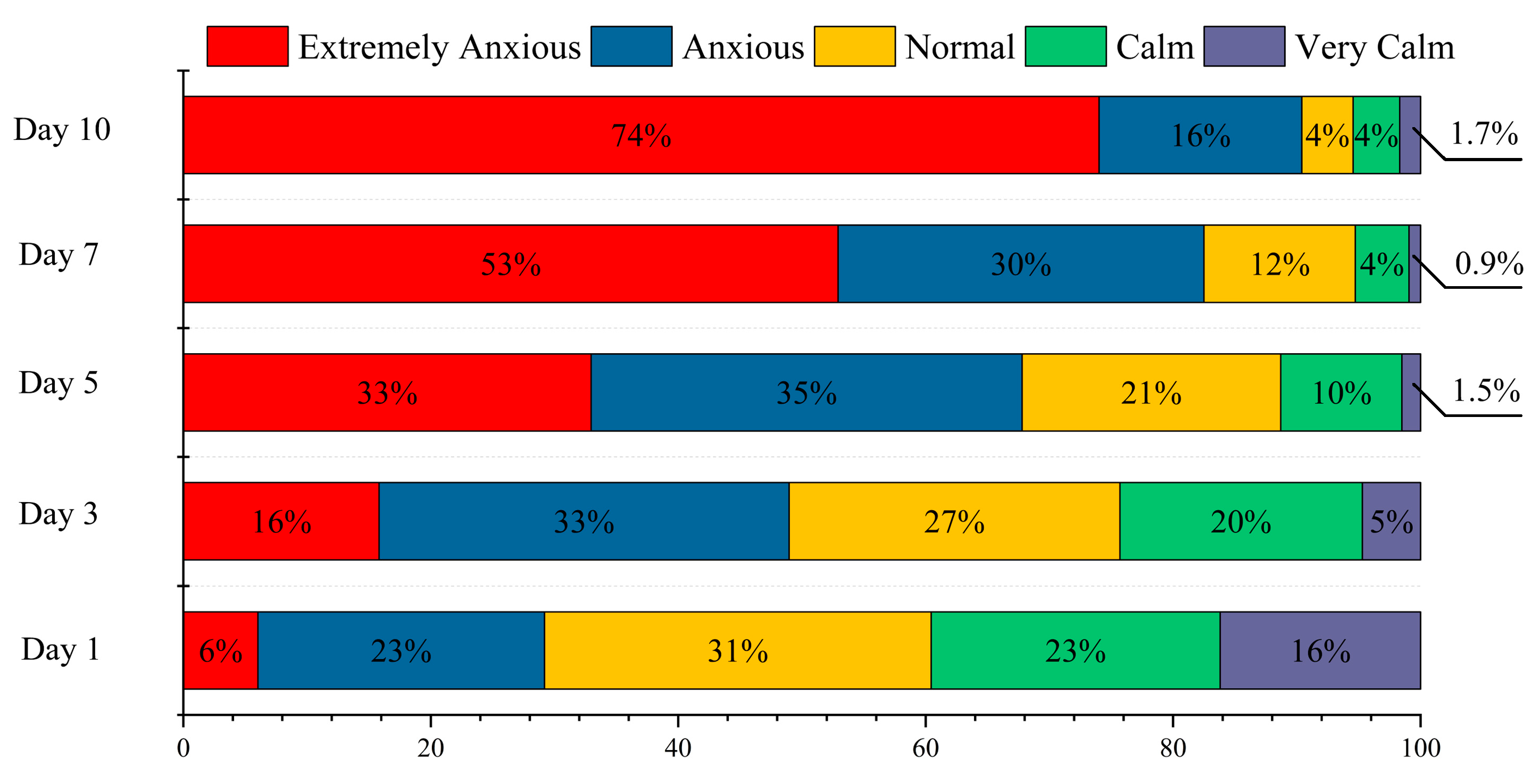
• During the initial stage of the SRtP in response to an accident on a cruise ship, passengers may experience five different emotional states with varying probabilities after they have gathered in a safety area. These states represent the initial distribution of emotions among the crowd.
• Over time, the emotional states of passengers undergo changes, influenced by varying probabilities of transitioning between different emotional states. The transition probability between two states is denoted by ${\alpha }_{ij}$, where $i$ and $j$ represent the scores of each state, respectively. Thus, the state transition matrix is given by Equation (1), where $P_{ij}$ is the transition probability from state $i$ to $j$.

To provide a clearer description of the passenger emotion contagion process, the following definitions are established:

$${\mathit{P}}_{ij}=\left[\begin{array}{ccccc}1-{\alpha }_{12}& {\alpha }_{12}& 0& 0& 0\\ {\alpha }_{21}& 1-{\alpha }_{21}-{\alpha }_{23}& {\alpha }_{23}& 0& 0\\ {\alpha }_{31}& {\alpha }_{32}& 1-{\alpha }_{31}-{\alpha }_{32}-{\alpha }_{34}& {\alpha }_{34}& 0\\ 0& 0& {\alpha }_{43}& 1-{\alpha }_{43}-{\alpha }_{45}& {\alpha }_{45}\\ 0& 0& 0& {\alpha }_{54}& 1-{\alpha }_{54}\end{array}\right],$$

(1)

Definition 1. 

Definition of the crowd’s emotional state. The emotional states of passengers can be divided into five categories at time $t$: extremely anxious, anxious, normal, calm and very calm, where $t$ represents the time point at which a specific phase concludes. The calculation of total number of people is shown in Equation (2), where $T$ is a constant total number of people. $E\left(t\right)$,$A\left(t\right)$, $N\left(t\right)$, $C\left(t\right)$ and $V\left(t\right)$ represent the number of people in extremely anxious, anxious, normal, calm and very calm states at time $t$.

$$T=E\left(t\right)+A\left(t\right)+N\left(t\right)+C\left(t\right)+V\left(t\right),$$

(2)

Definition 2. 

State transition events. A state transition involves a passenger transitioning from one state to another state. Let $T_{\left(i\right)}\left(t\right)$ and $T_{\left(j\right)}\left(t\right)$ represent the number of people in state $i$ and $j$ at time $t$; $T_{\left(i,j\right)}\left(∆t\right)$ represents the number of people whose status has changed from the state $i$ to $j$ in a time interval $∆t$. Thus, the number of people at time $t+∆t$ is given by Equations (3) and (4), where $T_{\left(i\right)}\left(t+∆t\right)$ and $T_{\left(j\right)}\left(t+∆t\right)$ are the number of people in state $i$ and $j$ at time $t+∆t$. Moreover, each person in a state can only transition to the nearest positive or negative state. For example, people in an anxious state can only transition to an extremely anxious state or a normal state, and cannot directly transition to a calm state or a very calm state. Only people in a normal state can directly transition to an extremely anxious state.

$$T_{\left(i\right)}\left(t+∆t\right)=T_{\left(i\right)}\left(t\right)-T_{\left(i,j\right)}(∆t),$$

(3)

$$T_{\left(j\right)}\left(t+∆t\right)=T_{\left(j\right)}\left(t\right)+T_{\left(i,j\right)}(∆t),$$

(4)

Definition 3. 

The source of infection is set as extremely anxious people and very calm people. The other states are not contagious.

Definition 4. 

Due to the impact of environment and time, people in any given state have the potential to transition to an adjacent state. For instance, even if people in a state of calm are not directly affected by someone experiencing extreme anxiety or people who are extremely calm, there exists a certain probability that they may transition to a very calm state or return to normal during the SRtP.

Definition 5. 

$R\left(E\right)$ denotes the coefficient of the rate of change, indicating how passengers in states other than the negative state are influenced by passengers experiencing extreme anxiety. For example, if $R\left(E\right)=2$, it implies that, under this influence, the probability of passengers transitioning to a negative state will become twice as high as the original probability. The function $R\left(E\right)$ can be characterized as a temporal and spatial function, represented by Equation (5), in which the variable $d$ signifies the linear distance between the passenger in a state of extreme anxiety and the target passenger.

$$R\left(E\right)=R_1\left(d,t\right) ,$$

(5)

$R\left(V\right)$ is the coefficient that represents the influence of individuals in a very calm state on the probability of transitioning the other person from a different state to a positive state.  $R\left(V\right)$ can be characterized as a temporal and spatial function, which can be expressed as Equation (6).

$$R\left(V\right)=R_2\left(d,t\right) ,$$

(6)

While the proposed model is not a traditional SIR model, it incorporates some similar concepts to describe the spread and evolution of emotions.

• Emotional State Classification: Unlike the infected state in the SIR model, this model categorizes emotional states into five distinct categories, ranging from extreme anxiety to very calm, and assigns scores from 1 to 5 to represent negative to positive emotional states. These different states can be thought of as different “infection” states within the crowd.
• State Transitions: Similar to the infection rate in the SIR model, the state transition probabilities ${\alpha }_{ij}$ in this model represent the likelihood of transitioning from one emotional state to another. These transition probabilities constitute a state transition matrix used to describe the spread and change of emotions between different emotional states, resembling the transmission process in the SIR model.
• Temporal Evolution: Like the SIR model, this model also considers the evolution over time. At the initial moment, passengers are in different emotional states, representing the initial distribution of emotions. Over time, passengers’ emotional states change influenced by the transition probabilities between different emotional states, akin to the infection spread process in the SIR model.

While this model is used to describe the spread and evolution of emotions, rather than the transmission of infectious diseases, it employs similar concepts of probabilistic transitions and state changes to describe how emotions propagate within a crowd in response to an emergency situation. The following advanced models also use the SIR model concept: the cyber-physical society-oriented recurrent emotional contagion (CPS–REC) model, stochastic event-based emotional contagion (SEEC) model, and emotional contagion-aware deep reinforcement learning model for antagonistic crowd simulation (ACSED) model (Appendix C).

The CPS–REC model takes into consideration the influence of emotional recurrence on the emotional contagion process, aiming to provide a more comprehensive understanding of crowd behavior. The formula of degree-based Mean-Field Equations is presented. These equations describe the dynamic evolution of the number of individuals within crowds while accounting for their heterogeneity.

The SEEC model introduces the occurrence intensity of infection/recovery events and constructs a state transition matrix to calculate the crowd state evolution. There are two categories within the crowd: susceptible individuals (i.e., individuals without negative emotions) and infected individuals (i.e., individuals with negative emotions) in this model.

The ACSED is a method designed to investigate the intricate interactions between emotions and decision-making within adversarial environments. Its emotional contagion module is constructed using the enhanced SIS model. What sets it apart from previous studies on emotional contagion is its integration of deep q network (DQN). ACSED leverages DQN to estimate individuals’ inclinations towards engaging in adversarial behavior, and then analyze the rationality underlying behavioral predictions.

2.2. Calculation of Crowd States

According to the relevant theories of the SIR Model [34], the system dynamics differential equations of the emotion model studied in this paper can be constructed. After time interval $∆t$, the population in each state can be calculated by the number of existing passengers, passengers transferred into the state, and passengers transferred out of the state. The following is the specific calculation formula:

$$\frac{dE}{dt}=\frac{E\left(t+∆t\right)-E\left(t\right)}{∆t}=N\left(t\right)·{\alpha }_{31}+A\left(t\right)·{\alpha }_{21}-E\left(t\right)·{\alpha }_{12},$$

(7)

$$\frac{dA}{dt}=\frac{A\left(t+∆t\right)-A\left(t\right)}{∆t}=E\left(t\right)·{\alpha }_{12}+N\left(t\right)·{\alpha }_{32}-A\left(t\right)·\left({\alpha }_{21}+{\alpha }_{23}\right),$$

(8)

$$\frac{dN}{dt}=\frac{N\left(t+∆t\right)-N\left(t\right)}{∆t}=A\left(t\right)·{\alpha }_{23}+C\left(t\right)·{\alpha }_{43}-N\left(t\right)·\left({\alpha }_{31}+{\alpha }_{32}+{\alpha }_{34}\right),$$

(9)

$$\frac{dC}{dt}=\frac{C\left(t+∆t\right)-C\left(t\right)}{∆t}=N\left(t\right)·{\alpha }_{34}+V\left(t\right)·{\alpha }_{54}-C\left(t\right)·\left({\alpha }_{43}+{\alpha }_{45}\right),$$

(10)

$$\frac{dV}{dt}=\frac{V\left(t+∆t\right)-V\left(t\right)}{∆t}=C\left(t\right)·{\alpha }_{45}-V\left(t\right)·{\alpha }_{54},$$

(11)

$$\frac{dE}{dt}+\frac{dA}{dt}+\frac{dN}{dt}+\frac{dC}{dt}+\frac{dV}{dt}=0,$$

(12)

$\frac{dE}{dt},\frac{dA}{dt},\frac{dN}{dt},\frac{dC}{dt}$ and $\frac{dV}{dt}$ represent the change rate of the number of people in each emotional state, respectively.

Equation (7) describes the rate of change of the number of people in state E over time. It considers the change in the number of people in this state as a result of passengers transitioning into this state from state N and state A (with probabilities ${\alpha }_{31}$ and ${\alpha }_{21}$, respectively) and those transitioning out of this state to the normal state A (with a probability of ${\alpha }_{12}$).

Equation (8) represents the rate of change in the number of people in state A over time. It accounts for people moving into this state from state E and state N (with probabilities ${\alpha }_{12}$ and ${\alpha }_{32}$, respectively) and those transitioning out to either state E or state N (with probabilities ${\alpha }_{21}$ and ${\alpha }_{23}$).

Equation (9) represents the rate of change in the number of people in state N over time. It considers individuals transitioning into this state from state A and state C (with probabilities ${\alpha }_{23}$ and ${\alpha }_{43}$, respectively) and those transitioning out to state E, state A, and state C (with probabilities ${\alpha }_{31}$, ${\alpha }_{32}$, and ${\alpha }_{34}$).

Equation (10) describes the rate of change for the number of people in state C over time. It accounts for individuals transitioning into this state from state N and state V (with probabilities ${\alpha }_{34}$ and ${\alpha }_{54}$, respectively) and transitioning out to state N and state V (with probabilities ${\alpha }_{43}$ and ${\alpha }_{45}$, respectively).

Equation (11) represents the rate of change in the number of people in state V over time. It considers individuals transitioning into this state from state C (with probabilities ${\alpha }_{45}$, respectively) and those transitioning out to the state C (with probabilities ${\alpha }_{54}$, respectively).

Equation (12) reflects the conservation of the total population within the emotional states. In other words, the sum of the rate of change of people in all emotional states equals zero, indicating that the total number of passengers remains constant over time.

These equations collectively model how the population in each emotional state changes over time based on transition probabilities between different emotional states.

As inferred from the preceding context, ${\alpha }_{ij}$ denotes the probability of transitioning from state $i$ to state $j$. In cases where a direct transition between two states is not feasible, ${\alpha }_{ij}$ is assigned a value of 0. When multiple passengers are in extreme emotional states, their influence on passengers in other states becomes cumulative. Let ${\alpha }_{ij}\left(t\right)$ represent the transition probability from state $i$ to state $j$ at time $t$, and let ${\alpha }_{ij}^{\prime }\left(t+∆t\right)$ signify the transition probability at time $t+∆t$. The relationship between ${\alpha }_{ij}(t)$ and ${\alpha }_{ij}^{\prime }\left(t+∆t\right)$ can be described by Equation (13).

$${\alpha }_{ij}^{\prime }\left(t+∆t\right)={\alpha }_{ij}\left(t\right)·\left[{\sum }_0^{T_E}R\left(E\right),i>j+{\sum }_0^{T_V}R\left(V\right),i<j+{\delta }_{ij}\right],$$

(13)

When $i>j$, this indicates the impact of passengers experiencing heightened anxiety levels, and the probability of transitioning towards negative emotional states is increased. At time $t+∆t$, the probability of state transition can be calculated as the sum of the rate of change coefficients for passengers in a state of extreme anxiety, multiplied by ${\alpha }_{ij}(t)$. Similarly, when $i<j$, the probability of state transition can be computed as the sum of rate of change coefficients for passengers in a notably calm state, again multiplied by ${\alpha }_{ij}(t)$. If $i=j$, it indicates the maintenance of the existing state. $T_E$ represents the number of passengers with extreme anxiety in the enclosed space, and $T_V$ represents the number of passengers who are very calm in the enclosed space. ${\delta }_{ij}$ represents 1 when $i=j$, and otherwise 0.

Normalization can be achieved by using Equation (14).

$${\alpha }_{ij}\left(t+∆t\right)=\frac{{\alpha }_{ij}^{\prime }\left(t+∆t\right)}{\sum _{j=1}^5{\alpha }_{ij}^{\prime }\left(t+∆t\right)} ,$$

(14)

where $i\in \left[\mathrm{1,5}\right]$, and $\sum _{j=1}^5{\alpha }_{ij}^{\prime }\left(t+∆t\right)$ represents the sum of the probabilities of the transition from the $i$ state to the other states.${\alpha }_{ij}\left(t+∆t\right)$ is the result after normalization.

3. Data and Analysis

3.1. Questionnaire Experimental Data

A significant portion of the existing research in this field has primarily concentrated on examining emotional contagion within relatively few hours, rendering it inadequate for application to the SRtP of cruise ships, which can span tens of days. This study is based on the emotional contagion model established in Section 2.1, and a questionnaire is developed using the control variable method (Appendix A). In the SRtP of a cruise ship, there is a scenario that all passengers are concentrated in safe areas, and the specification requires that the per capita area be no less than 2 m² [1]. In large cruise ships, the large public areas are about 1000 m², which can accommodate more than 500 passengers. In the event of a mass incident involving 500 passengers, the safety of the ship and passengers could be seriously compromised. By separating these areas into smaller zones, the number of passengers and crowd density can be effectively regulated. In order to study the influence of the total population and population density on emotional contagion in a small area, the control variates are used to establish different scenario control groups. In each scenario, the moment when all passengers complete the assembly in the safety area is recorded as moment $t=0$. The emotional state collected at 0:00 on the second day of the assembly is noted as the emotional state for Day 1. Similarly, the emotional states for Day 3, Day 5, Day 7, and Day 10 correspond to the emotional states collected at 0:00 on the day after these days. Scenario 1 to Scenario 3 set the density to $2 {\mathrm{m}}^2/\mathrm{p}\mathrm{e}\mathrm{r}\mathrm{s}\mathrm{o}\mathrm{n}$ and form a comparison group by gradually increasing the number of passengers. In scenarios 1, 4, and 5, maintain the total number of passengers unchanged, and create another comparison group by altering the crowd density. The scores are set for various emotional states from extreme anxiety to very calm states, ranging from 1 to 5 points, as shown in Table 1. In addition, to filter out questionnaires that have not been filled out diligently, an attention mechanism screening question will be included in the questionnaire. In total, 527 valid questionnaires were collected through the China Questionnaires Star Corporation. The results of the questionnaire are shown in Figure 2, Figure 3, Figure 4, Figure 5, Figure 6 and Figure 7.

Based on the data presented in Figure 2, it can be observed that, when guest rooms on a cruise ship are unavailable, most passengers (59.7%) prefer to seek refuge in restaurants, even if these restaurants are unable to offer regular catering services. Meanwhile, 18.6% of passengers tend to choose commercial areas as a place of refuge. Additionally, 21.7% of passengers tend to opt for gangway and stairway landings as a refuge.

Figure 3, Figure 4 and Figure 5 illustrate the emotional state distributions of three scenarios with equal density but varying total number of passengers. Figure 3 illustrates a notable surge in the population experiencing the extremely anxious state from Day 7 to Day 10, while the number of passengers in the very calm state decreases significantly from Day 1 to Day 3. Upon comparing Figure 3, Figure 4 and Figure 5, a discernible correlation emerges: changes in the number of passengers exert a significant influence upon their emotional states. It is observed that, with a constant density, an increase in the total number of passengers results in an upward trend and a higher peak value for the number of passengers in an extremely anxious state. However, the proportion of passengers in the very calm state exhibits a downward trend. The proportion of passengers in the anxious state fluctuates, with the peak time gradually advancing. Moreover, the fluctuation of the normal and calm states becomes gradually smooth over time.

Upon a comparison of Figure 3, Figure 6 and Figure 7, evident correlations surface between fluctuations in passenger density and resultant changes in their emotional states. Based on the data presented in these three figures, an obvious trend emerges wherein the proportion of individuals in an extremely anxious state experiences a pronounced surge from Day 7 through to Day 10. In contrast, during the initial Day 1 to Day 3 period, there is a discernible reduction in the proportion of individuals manifesting a very calm state. Despite the total number of passengers remaining constant, the peak number of those in the extremely anxious state decreases as the per capita area increases. Conversely, the peak number of the very calm state shows an upward trend. According to the data depicted in these three figures, two distinct trends become evident: as the per capita area increases, there is a recognizable postponement in the onset of the proportion of passengers in an anxious state; simultaneously, there is a corresponding decrease in the magnitude of the peak. The normal state exhibits relatively smooth fluctuation patterns. The state of calm also demonstrates relatively smooth fluctuations but with an increasing peak. Available data indicate a multifaceted correlation between population density and emotional states, with different emotional states exhibiting varying degrees of response to changes in population density.

3.2. Reliability and Validity Analysis of the Questionnaire

To ensure the quality of questionnaires, researchers often use reliability and validity measures [35]. When a questionnaire demonstrates good reliability and validity, it suggests that the data obtained from the questionnaire are internally consistent and accurate, making it suitable for further analysis. It is necessary to conduct a comprehensive evaluation of the reliability and validity of the questionnaire, as it consists of multiple scale questions.

Table A3. Reliability statistics.

Items		Corrected Item–Total Correlation (CITC)	Cronbach α
Gender		−0.026	0.916
Question3		0.060
Question4		0.063
Scenario 1 $\mathsf{\rho }=2 {\mathrm{m}}^2/\mathrm{p}\mathrm{e}\mathrm{r}\mathrm{s}\mathrm{o}\mathrm{n},\mathrm{n}=30$	Day1	0.505
	Day3	0.636
	Day5	0.726
	Day7	0.691
	Day10	0.563
Scenario 2 $\mathsf{\rho }=2 {\mathrm{m}}^2/\mathrm{p}\mathrm{e}\mathrm{r}\mathrm{s}\mathrm{o}\mathrm{n},\mathrm{n}=50$	Day1	0.580
	Day3	0.671
	Day5	0.737
	Day7	0.695
	Day10	0.567
Scenario 3 $\mathsf{\rho }=2 {\mathrm{m}}^2/\mathrm{p}\mathrm{e}\mathrm{r}\mathrm{s}\mathrm{o}\mathrm{n},\mathrm{n}=100$	Day1	0.602
	Day3	0.675
	Day5	0.673
	Day7	0.611
	Day10	0.484
Scenario 4 $\mathsf{\rho }=3 {\mathrm{m}}^2/\mathrm{p}\mathrm{e}\mathrm{r}\mathrm{s}\mathrm{o}\mathrm{n},\mathrm{n}=30$	Day1	0.536
	Day3	0.596
	Day5	0.670
	Day7	0.691
	Day10	0.566
Scenario 5 $\mathsf{\rho }=4 {\mathrm{m}}^2/\mathrm{p}\mathrm{e}\mathrm{r}\mathrm{s}\mathrm{o}\mathrm{n},\mathrm{n}=30$	Day1	0.505
	Day3	0.525
	Day5	0.631
	Day7	0.635
	Day10	0.579

Cronbach α (Standardized): 0.933.

presents the reliability calculation table, which shows that the reliability coefficient value of the Cronbach α is 0.916. This value is greater than 0.9, indicating that the reliability quality of the research data is high [36]. Additionally, the value of the Corrected Item–Total Correlation (CITC) is also analyzed to indicate the degree of association between the items. It is found that the CITC values corresponding to questions 1, 3, and 4 are all less than 0.2. This suggests that the relationships between these three questions and the rest of the analysis items are weak. This is mainly due to the fact that these questions involve pre-test analysis. Overall, the reliability of the research data enhances the credibility of the study’s findings.

Validity research is used to analyze whether a research item is reasonable and meaningful. The validity level of data can be analyzed through indicators such as the Kaiser–Meyer–Olkin (KMO), commonality, variance interpretation rate, and factor load coefficient values. The KMO value is used to determine the suitability of information extraction, the commonality value is used to exclude unreasonable research items, the variance interpretation rate value is used to explain the level of information extraction, and the factor load coefficient is used to measure the corresponding relationship between factors (dimensions) and items [37]. The results of the validity analysis are presented in

Table A4. Validity analysis.

Items		Factor Loadings					Communalities
		Factor 1	Factor 2	Factor 3	Factor 4	Factor 5
Gender		0.025	−0.083	−0.015	0.022	0.647	0.427
Question3		0.044	−0.060	0.057	0.126	−0.631	0.423
Question4		0.032	−0.036	0.095	0.055	0.440	0.208
Scenario 1 $\mathsf{\rho }=2 {\mathrm{m}}^2/\mathrm{p}\mathrm{e}\mathrm{r}\mathrm{s}\mathrm{o}\mathrm{n},$ n = 30	Day1	−0.135	0.501	0.266	0.622	−0.054	0.731
	Day3	0.203	0.372	0.236	0.723	−0.022	0.758
	Day5	0.460	0.219	0.326	0.645	−0.000	0.782
	Day7	0.663	0.056	0.322	0.489	0.017	0.785
	Day10	0.774	−0.091	0.247	0.272	−0.001	0.742
Scenario 2 $\mathsf{\rho }=2 {\mathrm{m}}^2/\mathrm{p}\mathrm{e}\mathrm{r}\mathrm{s}\mathrm{o}\mathrm{n},$ n = 50	Day1	−0.147	0.409	0.610	0.464	−0.000	0.776
	Day3	0.048	0.300	0.682	0.436	−0.006	0.748
	Day5	0.377	0.163	0.666	0.356	0.066	0.743
	Day7	0.574	−0.008	0.605	0.250	0.037	0.759
	Day10	0.721	−0.124	0.465	0.052	−0.034	0.756
Scenario 3 $\mathsf{\rho }=2 {\mathrm{m}}^2/\mathrm{p}\mathrm{e}\mathrm{r}\mathrm{s}\mathrm{o}\mathrm{n},$ n = 100	Day1	−0.080	0.298	0.819	0.235	0.049	0.823
	Day3	0.139	0.196	0.876	0.136	0.058	0.847
	Day5	0.304	0.087	0.850	0.057	0.006	0.826
	Day7	0.480	−0.056	0.766	−0.037	−0.027	0.822
	Day10	0.648	−0.193	0.520	−0.099	−0.083	0.743
Scenario 4 $\mathsf{\rho }=3 {\mathrm{m}}^2/\mathrm{p}\mathrm{e}\mathrm{r}\mathrm{s}\mathrm{o}\mathrm{n},$ n = 30	Day1	−0.073	0.815	0.240	0.195	−0.052	0.768
	Day3	0.171	0.851	0.131	0.105	−0.049	0.784
	Day5	0.465	0.716	0.120	0.100	0.048	0.755
	Day7	0.719	0.505	0.123	0.020	0.018	0.787
	Day10	0.859	0.255	0.051	−0.039	0.030	0.807
Scenario 5 $\mathsf{\rho }=4 {\mathrm{m}}^2/\mathrm{p}\mathrm{e}\mathrm{r}\mathrm{s}\mathrm{o}\mathrm{n},$ n = 30	Day1	−0.092	0.824	0.162	0.244	−0.018	0.773
	Day3	0.110	0.858	0.046	0.120	−0.053	0.767
	Day5	0.438	0.762	0.027	0.082	0.002	0.780
	Day7	0.669	0.586	−0.007	0.052	0.026	0.794
	Day10	0.834	0.350	−0.020	0.007	0.048	0.821
Eigenvalues (Rotated)		5.958	5.615	5.426	2.488	1.051	-
Variance (Rotated)		21.277%	20.054%	19.379%	8.885%	3.752%	-
Cum. Variance (Rotated)		21.277%	41.331%	60.710%	69.594%	73.346%	-
KMO		0.928					-
p-value of Bartlett’s Test of Sphericity		$<0.001$					-

. It can be seen from the table that most research items have commonality values over 0.4, except for question 4. This indicates effective extraction of research item information. Question 4 is less than 0.4, indicating that the research item information is not able to be effectively expressed, mainly because it involves the collection of intentions. The variance interpretation rates of the five factors are 21.3%, 20.1%, 19.4%, 8.9%, and 3.8%, respectively. The cumulative variance interpretation rates after rotation are 73.346% > 50%. This means that the amount of information in the research item can be effectively extracted. If the p-value of Bartlett’s Test of Sphericity is less than 0.05, it indicates that it has passed the Bartlett sphericity test and has validity [37]. The p-value in this study is less than 0.001, indicating that the questionnaire has successfully undergone validity analysis, confirming its adequate validity.

3.3. Correlation Analysis

Correlation analysis refers to the analysis of two or more correlated variable elements, which is used to measure the degree of correlation between two variable factors. Based on a designated control group, the study examines the correlations between population density and emotional states at different times, as well as the correlations between total population and emotional states at different times.

Table 2. Non-parametric test analysis for different densities.

Items	ρMedian(Q1, Q3)		Mann–Whitney U	Mann–Whitney z	p
	2.0	3.0
Day 1 Emotional States	4.000 (3.0, 5.0)	4.000 (4.0, 5.0)	666,584.500	−9.116	$<0.01$
Day 3 Emotional States	3.000 (2.0, 4.0)	4.000 (3.0, 4.0)	601,989.000	−12.634	$<0.01$
Day 5 Emotional States	2.000 (2.0, 3.0)	3.000 (3.0, 4.0)	564,124.000	−14.654	$<0.01$
Day 7 Emotional States	2.000 (1.0, 2.0)	2.000 (2.0, 3.0)	549,802.500	−15.549	$<0.01$
Day 10 Emotional States	1.000 (1.0, 2.0)	2.000 (1.0, 3.0)	586,807.000	−12.559	$<0.01$

shows the results of a Non-parametric test comparing emotional states across different population densities. $Q_1$ and $Q_3$ denote the lower quartile and upper quartile, respectively. The differences in density can be seen for five emotional states at five different time points. It is evident that the density values can be divided into two groups, with values of 2.0 and 3.0, respectively. The second and third columns present the lower quartile, median, and upper quartile values for daily emotional states under two different densities: $2 {\mathrm{m}}^2/\mathrm{p}\mathrm{e}\mathrm{r}\mathrm{s}\mathrm{o}\mathrm{n}$ and $3 {\mathrm{m}}^2/\mathrm{p}\mathrm{e}\mathrm{r}\mathrm{s}\mathrm{o}\mathrm{n}$. To illustrate, see the data in the first row of the second column, where, under a density of $2 {\mathrm{m}}^2/\mathrm{p}\mathrm{e}\mathrm{r}\mathrm{s}\mathrm{o}\mathrm{n}$, the median for emotional score in Day 1 registers as 2, the lower quartile as 3, and the upper quartile as 5. Notably, within the second and third columns, instances arise where the median is equal to either the lower or upper quartile. This occurrence signifies that, for a specific emotional state, the count of individuals with that emotional score encompasses at least 25% of the total population. For example, in the first row of the third column, both the median and lower quartile are reported as 4. This observation implies that, under the density of $3 {\mathrm{m}}^2/\mathrm{p}\mathrm{e}\mathrm{r}\mathrm{s}\mathrm{o}\mathrm{n}$, when individuals are arranged in ascending order based on their emotional scores, those scoring 4 represent a range spanning at least 25% to 50% of the total population.

To analyze these groups, a Mann–Whitney test is needed. However, if there are more than two groups, a Kruskal–Wallis test is necessary [38]. The results indicate that the emotional states at all five time points vary significantly across different population densities (p < 0.05). This suggests that samples with different densities display significant differences in emotional states at all five time points. Further analysis reveals the following:

(1)

Based on the study results, it appears that population density has a significant effect on emotional state on Day 1, with a p-value less than 0.01 indicating a significant difference. Additionally, the comparison of median differences suggests that the source of the differences is due to different data distributions. Figure 8 shows a block diagram of emotional state data at different densities, revealing that the mean emotional state on the first day is around 4.1 when the density is $2 {\mathrm{m}}^2/\mathrm{p}\mathrm{e}\mathrm{r}\mathrm{s}\mathrm{o}\mathrm{n}$, while it is around 4 when the density is $3 {\mathrm{m}}^2/\mathrm{p}\mathrm{e}\mathrm{r}\mathrm{s}\mathrm{o}\mathrm{n}$. These findings suggest that higher population densities may lead to a decrease in emotional state on Day 1.

(2)

The population density shows a significance level for the emotional states on Day 5, and the mean value of $2 {\mathrm{m}}^2/\mathrm{p}\mathrm{e}\mathrm{r}\mathrm{s}\mathrm{o}\mathrm{n}$ is significantly lower than that of $3 {\mathrm{m}}^2/\mathrm{p}\mathrm{e}\mathrm{r}\mathrm{s}\mathrm{o}\mathrm{n}$.

(3)

The analysis shows that population density has a significant impact on emotional states on Day 7. Based on Figure 8, it can be observed that, when the population density is $2 {\mathrm{m}}^2/\mathrm{p}\mathrm{e}\mathrm{r}\mathrm{s}\mathrm{o}\mathrm{n}$, the mean emotional state score on Day 7 is approximately 2.1. However, the mean emotional state score on Day 7 is around 2.5 when the density is $3 {\mathrm{m}}^2/\mathrm{p}\mathrm{e}\mathrm{r}\mathrm{s}\mathrm{o}\mathrm{n}$. From these two mean values, it can be inferred that, when the population density is $2 {\mathrm{m}}^2/\mathrm{p}\mathrm{e}\mathrm{r}\mathrm{s}\mathrm{o}\mathrm{n}$, the emotional state for Day 7 is more likely to be distributed with a score of 2.

(4)

Passenger density exhibits a notable correlation with emotional states on Day 10. The median differences further demonstrate that the average density of $2 {\mathrm{m}}^2/\mathrm{p}\mathrm{e}\mathrm{r}\mathrm{s}\mathrm{o}\mathrm{n}$ is significantly lower than that of $3 {\mathrm{m}}^2/\mathrm{p}\mathrm{e}\mathrm{r}\mathrm{s}\mathrm{o}\mathrm{n}$. Specifically, in the scenario where the density is $3 {\mathrm{m}}^2/\mathrm{p}\mathrm{e}\mathrm{r}\mathrm{s}\mathrm{o}\mathrm{n}$, there appears to be a higher count of individuals exhibiting comparatively lower emotional scores. This observation is particularly evident when contrasting it with the crowd characterized by a density of $2 {\mathrm{m}}^2/\mathrm{p}\mathrm{e}\mathrm{r}\mathrm{s}\mathrm{o}\mathrm{n}$.

Through the Mann–Whitney test, it can be found that the samples with different densities showed significant differences in emotional states at different days.

Table 3. Non-parametric test analysis for different total population samples.

Items	nMedian (Q1, Q3)			Kruskal-Wallis H	p
	30.0	50.0	100.0 (n = 527)
Day 1 Emotional States	4.000 (4.0, 5.0)	4.000 (3.0, 5.0)	3.000 (2.0, 4.0)	−501.523	1.000
Day 3 Emotional States	4.000 (3.0, 4.0)	3.500 (3.0, 4.0)	3.000 (2.0, 3.0)	−587.672	1.000
Day 5 Emotional States	3.000 (2.0, 4.0)	3.000 (2.0, 4.0)	2.000 (1.0, 3.0)	−747.935	1.000
Day 7 Emotional States	2.000 (2.0, 3.0)	2.000 (1.0, 3.0)	1.000 (1.0, 2.0)	−305.579	1.000
Day 10 Emotional States	2.000 (1.0, 2.0)	2.000 (1.0, 2.0)	1.000 (1.0, 2.0)	41.962	$<0.01$

presents the results of a non-parametric test for the emotional states of different population samples, indicating the differences in the total number of passengers in five emotional states at different days. The Kruskal–Wallis test is used to analyze the data since the total number of samples exceeds two groups. The results show that there are no significant differences in emotional states among different population samples on Day 1, Day 3, Day 5, and Day 7 ($p>0.05$), indicating consistent emotional patterns across these time periods. Further analysis is required from the box plots. Figure 9 shows the box plots of emotional states for different population samples. However, significant differences (p < 0.01) are observed in one emotional state on Day10, suggesting that the emotional state differs among different total sample sizes on this day. Based on Figure 9, the following results can be obtained.

(1)

Regarding the emotional state scores on Day 1 shown in Figure 9, as the total number of passengers changes from 30 to 50, the lowest score decreases from 3 to 2. Simultaneously, the interquartile range, representing the concentration interval, narrows from (4, 5) to (3, 4), and the mean score also decreases. When the number of passengers changes from 50 to 100, the concentration interval expands from (3, 4) to (2, 4), and the mean score decreases further. A decrease in the mean implies a rise in the proportion of passengers with lower scores. Therefore, overall, an increase in the total number of passengers has a negative impact on the emotional state on Day 1.

(2)

For the emotional state scores on Day 3, as the total number of passengers changes from 30 to 50, the concentration interval expands from (3, 4) to (2, 4), and the mean score decreases significantly. When the number of passengers changes from 50 to 100, the lowest score decreases from 2 to 1, the concentration interval narrows from (2, 4) to (2, 3), and the mean score also decreases. Thus, an increase in the number of passengers has a negative effect on the emotional state on Day 3.

(3)

Regarding the emotional state scores on Day 5, as the number of passengers changes from 30 to 50, the extreme value and concentration interval remain the same, but the mean score decreases, indicating that the group is shifting towards lower emotional state scores. When the number of passengers changes from 50 to 100, the concentration interval expands from (2, 3) to (1, 3), and the mean score decreases further. This suggests that an increase in the total number of passengers has a negative impact on the emotional state on Day 5.

(4)

For the emotional state scores on Day 7, as the number of passengers change from 30 to 50, the concentration interval decreases from (2, 3) to (1, 2), and the mean score decreases. When the number of passengers changes from 50 to 100, the extreme value and concentration interval remain the same, but the mean score decreases, indicating that the group is shifting towards lower emotional state scores. Therefore, an increase in the number of people has a negative effect on the emotional state on Day 7.

(5)

Regarding the emotional state scores on Day 10, as the number of passengers change from 30 to 50, the extreme value and concentration interval remain the same, but the mean score slightly decreases. When the number of passengers change from 50 to 100, the highest score decreases from 3 to 2, the concentration interval remains the same, and the mean score decreases. Thus, an increase in the number of passengers has a negative impact on the emotional state on Day 10.

In summary, an increase in the number of passengers will lead to a decrease in the emotional score, reflecting a negative impact on emotions. Moreover, different numbers of passengers may result in different ranges of emotional fluctuations.

Table 4. Summary table of model regression coefficients for adjacent time.

Items 1	Items 2	Unstandardized Path Coefficient	SE	z (CR)	p	Standardized Path Coefficient
Day 7 Emotional States	Day 10 Emotional States	0.741	0.012	63.026	$<0.001$	0.775
Day 5 Emotional States	Day 7 Emotional States	0.748	0.012	61.752	$<0.001$	0.769
Day 3 Emotional States	Day 5 Emotional States	0.758	0.012	61.104	$<0.001$	0.766
Day 1 Emotional States	Day 3 Emotional States	0.784	0.012	64.018	$<0.001$	0.780

and

Table 5. Summary table of model regression coefficients for non-adjacent time.

Items 1	Items 2	Unstandardized Path Coefficient	SE	z (CR)	p	Standardized Path Coefficient
Day 1 Emotional States	Day 10 Emotional States	0.200	0.018	11.381	$<0.001$	0.216
Day 1 Emotional States	Day 7 Emotional States	0.433	0.017	25.671	$<0.001$	0.447
Day 1 Emotional States	Day 5 Emotional States	0.630	0.015	42.016	$<0.001$	0.633
Day 1 Emotional States	Day 3 Emotional States	0.784	0.012	64.019	$<0.001$	0.780

are summary tables of model regression coefficients, where $SE$ represents standard error, $z\left(CR\right)$ represents critical ratio, and $p$ represents significance. As can be seen in Table 4, a significant and positive impact relationship is revealed between emotional states at adjacent time points. The standardized path coefficients, approximately 0.7, emphasize this relationship.

Furthermore, an assessment of emotional states on Day 1 and subsequent days was executed using standardized path analysis, as depicted in Table 5. The outcomes of this analysis show a gradual reduction in the strength of the relationship between emotional states on the initial day and those on all subsequent days.

In conclusion, these results suggest two key points. Firstly, the emotional states from the prior time period can serve as valuable indicators for predicting emotional states in immediate successive time periods. Notably, the substantial standardized path coefficients of around 0.7 reinforce this predictive relationship. Secondly, while the emotional states on Day 1 provide predictive utility for subsequent days, this predictability diminishes as the temporal lag increases. Hence, direct inference of emotional states on Days 5, 7, and 10 from the emotional state of Day 1 is not feasible.

To address this limitation, an iterative forecasting approach emerges as a viable strategy. Although direct prediction of emotional states on later days from the emotional state of Day 1 is constrained, a step-by-step iterative approach can be employed. This iterative forecasting method would involve predicting emotional states on Day 2 based on Day 1, then using the predicted Day 2 emotional state to predict Day 3, and so forth. This approach accommodates the temporal dynamics of emotional state progression and gains more accurate predictions.

4. Simulation and Results Analysis

The questionnaire data collected are employed as machine learning samples to construct a random forest algorithm for prediction purposes. From the model constructed in Section 2.1, it can be seen that the prediction essentially consisted of a classification problem. Random forest is a commonly used method in machine learning that employs decision trees for data analysis. The random forest (RF) algorithm can avoid overfitting to a certain extent in classification problems and is suitable for parallel operations [39]. Finally, testing and visualization are conducted through simulation.

4.1. Model Parametric Construction

4.1.1. Initial State of Each Scenario

• Grid division of the scenarios

The emotional contagion within a population in physical space is closely related to the distribution of individuals. To avoid excessively long queues in the setting, the grid of the scenarios determines the number of columns by taking the square root of the total number of passengers and rounding it down, while the number of rows is determined by rounding it up.

2.

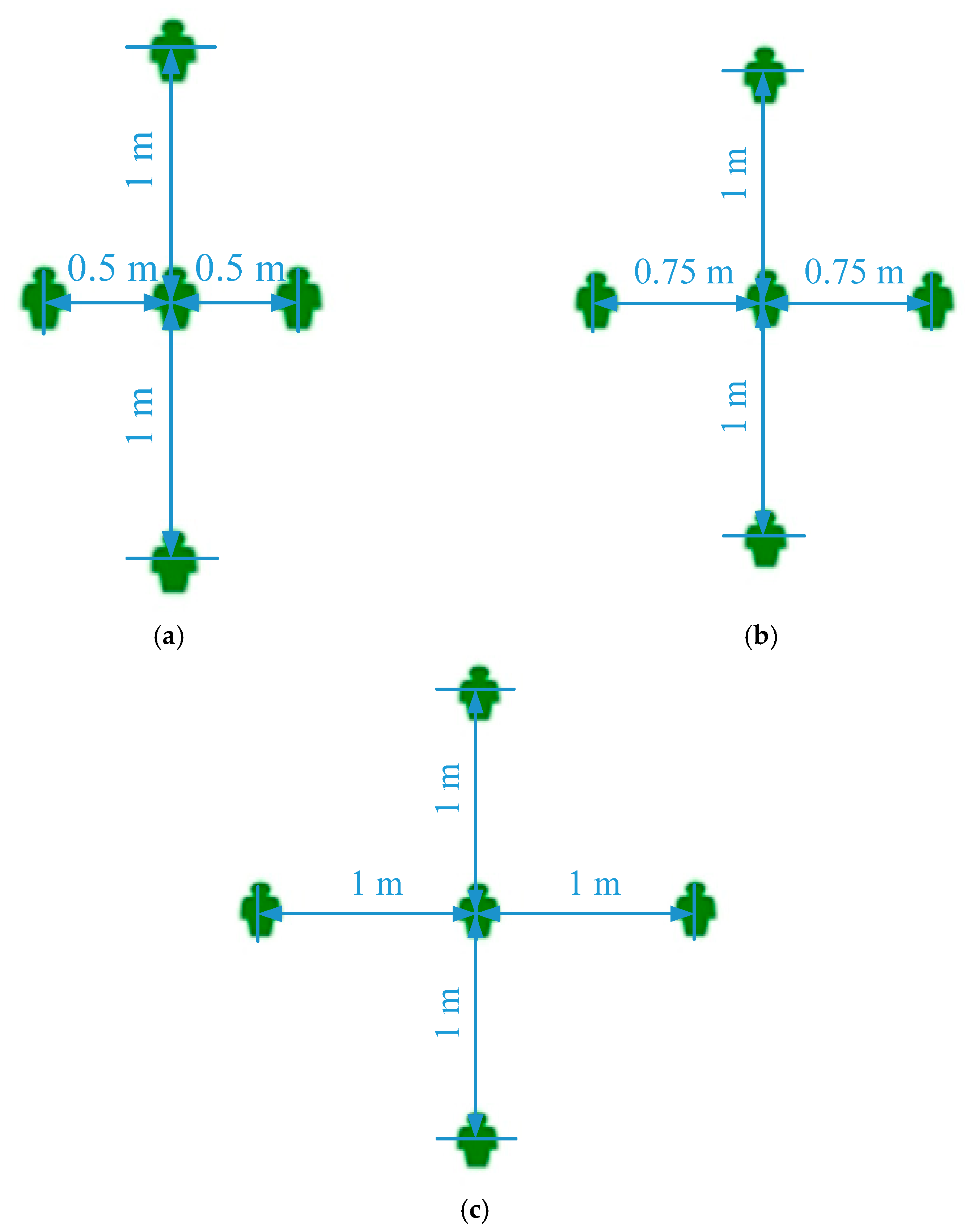
Distance between passengers

Passenger spatial distribution is categorized according to different densities, as illustrated in Figure 10.

For a density of $2 {\mathrm{m}}^2/\mathrm{p}\mathrm{e}\mathrm{r}\mathrm{s}\mathrm{o}\mathrm{n}$, the spatial allocation entails a longitudinal gap of 1 m in the front–back direction and a lateral gap of 0.5 m in the left–right direction.

In the case of a density of $3 {\mathrm{m}}^2/\mathrm{p}\mathrm{e}\mathrm{r}\mathrm{s}\mathrm{o}\mathrm{n}$, the spatial distribution involves a longitudinal gap of 1 m in the front–back direction, coupled with a lateral gap of 0.75 m in the left–right direction.

When considering a density of $4 {\mathrm{m}}^2/\mathrm{p}\mathrm{e}\mathrm{r}\mathrm{s}\mathrm{o}\mathrm{n}$, the spatial configuration encompasses a longitudinal gap of 1 m in the front–back direction and a lateral gap of 1 m in the left–right direction. The personnel arrangement shape in each scene should be as close to a square as possible.

3.

Initial number of passengers and initial transition probabilities

The initial passenger count is determined by rounding the proportions of individuals in various emotional states on Day 1, as per the statistical data collected from the surveys. Priority is given to preserving the proportion of individuals in extreme emotional states, with subsequent adjustments made for individuals in other states.

The initial values for the emotion transition rates were set based on data gathered through a questionnaire. However, it should be noted that the respondents may not have fully understood the impact of emotional contagion among passengers in different scenarios, so the data may be more biased toward passenger emotional transitions. The rate of conversion for each emotion from Day 1 to Day 3 was calculated to determine the initial value for each emotion conversion rate. For example, in the questionnaire for Scenario 1, there were 67 passengers recorded in a normal state on Day 1. On Day 3, 1 passenger transitioned to the extreme anxiety state, 25 passengers transitioned to the anxious state, 22 passengers remained in the normal state, and 14 passengers transitioned to the calm state. If the transition probabilities at Day 1 are not affected by extreme emotions, the values of ${(\alpha }_{31},{\alpha }_{32},{\alpha }_{33},{\alpha }_{34},{\alpha }_{35})$ are (0.1, 0.4, 0.3, 0.2, 0).

The specific initial passenger numbers and transition probabilities for each scenario are as follows:

$${\mathit{T}}_1=\left[\begin{array}{ccccc}0& 2& 3& 13& 12\end{array}\right],$$

(15)

$${\mathit{T}}_2=\left[\begin{array}{ccccc}1& 5& 14& 20& 10\end{array}\right],$$

(16)

$${\mathit{T}}_3=\left[\begin{array}{ccccc}6& 26& 30& 22& 16\end{array}\right],$$

(17)

$${\mathit{T}}_4=\left[\begin{array}{ccccc}0& 2& 5& 12& 11\end{array}\right],$$

(18)

$${\mathit{T}}_5=\left[\begin{array}{ccccc}0& 2& 5& 10& 13\end{array}\right],$$

(19)

$${\mathit{P}}_1=\left[\begin{array}{ccccc}0& 1& 0& 0& 0\\ 0.32& 0.63& 0.05& 0& 0\\ 0.01& 0.39& 0.37& 0.23& 0\\ 0& 0& 0.59& 0.39& 0.02\\ 0& 0& 0& 0.8& 0.2\end{array}\right],$$

(20)

$${\mathit{P}}_2=\left[\begin{array}{ccccc}0.63& 0.37& 0& 0& 0\\ 0.35& 0.6& 0.05& 0& 0\\ 0.01& 0.5& 0.38& 0.11& 0\\ 0& 0& 0.65& 0.33& 0.02\\ 0& 0& 0& 0.81& 0.19\end{array}\right],$$

(21)

$${\mathit{P}}_3=\left[\begin{array}{ccccc}0.88& 0.12& 0& 0& 0\\ 0.4& 0.56& 0.04& 0& 0\\ 0.04& 0.58& 0.32& 0.06& 0\\ 0& 0& 0.67& 0.28& 0.05\\ 0& 0& 0& 0.79& 0.21\end{array}\right],$$

(22)

$${\mathit{P}}_4=\left[\begin{array}{ccccc}0.4& 0.6& 0& 0& 0\\ 0.44& 0.53& 0.03& 0& 0\\ 0& 0.29& 0.56& 0.15& 0\\ 0& 0& 0.5& 0.48& 0.02\\ 0& 0& 0& 0.67& 0.33\end{array}\right],$$

(23)

$${\mathit{P}}_5=\left[\begin{array}{ccccc}0.6& 0.4& 0& 0& 0\\ 0.27& 0.63& 0.1& 0& 0\\ 0.02& 0.25& 0.6& 0.13& 0\\ 0& 0& 0.42& 0.56& 0.02\\ 0& 0& 0& 0.54& 0.46\end{array}\right],$$

(24)

where $({\mathit{T}}_1,{\mathit{T}}_2,{\mathit{T}}_3,{\mathit{T}}_4,{\mathit{T}}_5)$ represent the initial number of passengers from scenario 1 to scenario 5 and $({\mathit{P}}_1,{\mathit{P}}_2,{\mathit{P}}_3,{\mathit{P}}_4,{\mathit{P}}_5)$ represent the transition probabilities from scenario 1 to scenario 5.

4.1.2. Other Model Parameters

According to the definition in the previous part, $R\left(E\right)$ and $R\left(V\right)$ are functions of distance and time. Emotional transmission is a complex phenomenon that is influenced by a combination of factors, including non-verbal communication, social influences, and group effects. There are fewer studies on the expression of specific functions between emotional contagion and distance and time. However, some research suggests that emotional contagion may be more likely to occur when people are in close proximity to each other [33]. Emotional contagion can also spread quickly in a relatively short period of time and spread further over time [40]. To enhance the analytical and computational processes while ensuring a tractable problem formulation, we introduce postulates for the functions $R\left(E\right)$ and $R\left(V\right)$, as delineated below:

$$R\left(E\right)=\frac{a_1}{d_1}+b_1\times t^2 ,$$

(25)

$$R\left(V\right)=\frac{a_2}{d_2}{+b}_2\times t^2 ,$$

(26)

where $a_1,a_2,b_1,b_2$ are coefficients greater than 0, of which all initial values are 1. $d_1$ and $d_2$ are the linear distances from passengers in the extremely anxious state to passengers in the very calm state. $d_1$ denotes the Euclidean distance between a passenger and one of the passengers exhibiting extreme anxiety. Conversely, $d_2$ represents the Euclidean distance between a passenger and one of the passengers displaying significant calmness.

4.2. Algorithm Flow

Based on an improved weighted random forest algorithm [41,42,43,44,45], the prediction problem of emotional contagion in the SRtP process of cruise ships could be constructed as a classification problem. Figure 11 is the algorithm flowchart and the detailed process is as follows:

Step 1: Data pre-processing of the original dataset, mainly including data cleaning and feature encoding.

Step 2: Repeat sampling with playback is used to extract $K+1$ datasets, wherein K constitutes a training set and the other constitutes a test set, and the capacity of each dataset is equal to the total sample capacity, and where the value of $K$ is 100.

Step 3: By simulating a realistic area separation, each scene is sampled without replacement from the sample set based on the predetermined number of passengers until the collection is complete. Each sample is taken as a sub-training set.

Step 4: Scenario categorization. Each decision tree is divided into five scenarios set by the questionnaire. $F_m$ represents the degree of similarity between the scenario $m$ and the scenario $i$. The smaller the $F_m$, the more similar it is to the training scenario $i$, which is introduced into this scenario. The specific calculation of $F_m$ is as follows:

$$F_m={\epsilon }_1·\frac{\left|{\rho }_m-{\rho }_i\right|}{{\rho }_i}+{\epsilon }_2·\frac{\left|n_m-n_i\right|}{n_i} ,$$

(27)

It is assumed that the parameters for the passenger m of Day 1 to be classified are (${\rho }_m$,$n_m$,$e_m$), where ${\rho }_m$ represents the population density of the group in which the passenger to be classified belongs, $n_m$ is the total number of passengers in the group, $e_m$ indicates the emotional state score, ${\mathsf{\rho }}_i$ represents the population density of the scenario $i$, and ${\mathrm{n}}_i$ is the total number of passengers in scenario $i$. ${\epsilon }_1$ and ${\epsilon }_2$ are weight coefficients with an initial value of 0.5, which are adjusted through computational calculations. If multiple scenarios have equal $F_m$ values, they participate in the subsequent voting session together.

Step 5: Emotion score calculation and classification result statistics. According to each possible transition direction and the corresponding infection rate equations given in the previous infectious disease model, the next stage score can be calculated. The results of the calculations are then weighted and disaggregated into statistics.

$G_k$ is the weighting coefficient for the k-th training set which can be calculated by Equation (28):

$$G_k={\sigma }_1·\frac{n_k-n_{k1}}{n_k}+{\sigma }_2·\frac{n_k-n_{k5}}{n_k} ,$$

(28)

where ${\sigma }_1$ and ${\sigma }_2$ are weight coefficients with an initial value of 0.5, which are adjusted through computational calculations. $n_k$ is the total number of passengers in the k-th training set scenario. $n_{k1}$ is the number of passengers with a score of 1 in the k-th training set, and $n_{k5}$ is the number of passengers with a score of 5 in the k-th training set. By using comprehensive weighting coefficients to vote on all sub-training sets, then classification results could be obtained.

Step 6: Determining whether the requirements are met. Compare the final proportions of each emotional state with the test set. If the results do not meet the specified requirements, make parameter adjustments and return to step 4. If the results meet the requirements, output the final result.

Table 6. Values of the parameters.

Parameters	Values
$\mathrm{b}\mathrm{a}\mathrm{g}\mathrm{S}\mathrm{i}\mathrm{z}\mathrm{e}\mathrm{P}\mathrm{e}\mathrm{r}\mathrm{c}\mathrm{e}\mathrm{n}\mathrm{t}$	100
$\mathrm{b}\mathrm{a}\mathrm{t}\mathrm{c}\mathrm{h}\mathrm{S}\mathrm{i}\mathrm{z}\mathrm{e}$	100
$\mathrm{n}\mathrm{u}\mathrm{m}\mathrm{I}\mathrm{t}\mathrm{e}\mathrm{r}\mathrm{a}\mathrm{t}\mathrm{i}\mathrm{o}\mathrm{n}\mathrm{s}$	100
$\mathrm{n}\_\mathrm{e}\mathrm{s}\mathrm{t}\mathrm{i}\mathrm{m}\mathrm{a}\mathrm{t}\mathrm{o}\mathrm{r}\mathrm{s}$	500
$\mathrm{m}\mathrm{a}\mathrm{x}\_\mathrm{d}\mathrm{e}\mathrm{p}\mathrm{t}\mathrm{h}$	5

shows the values of the parameters (e.g., number of trees, etc.) of the applied random forest algorithm.

4.3. Results and Discussion

4.3.1. Evaluation of Models

According to the previous study, the situation on Day 1 is used as the initial value for prediction learning over the following days. The confusion matrix of the model is shown in Figure 12, Figure 13, Figure 14 and Figure 15, with the horizontal axis representing the predicted emotional score and the vertical axis representing the actual emotional score. The confusion matrix diagram can clearly reflect the accuracy of predicting various emotional states and the distribution of misjudgments.

From Figure 12, Figure 13, Figure 14 and Figure 15, it is evident that the prediction accuracy for the extreme anxiety and very calm states is high. The prediction accuracy for the very calm state gradually improves over time, especially on Day 10, where it reaches 100%. There are several reasons for this result:

(1)

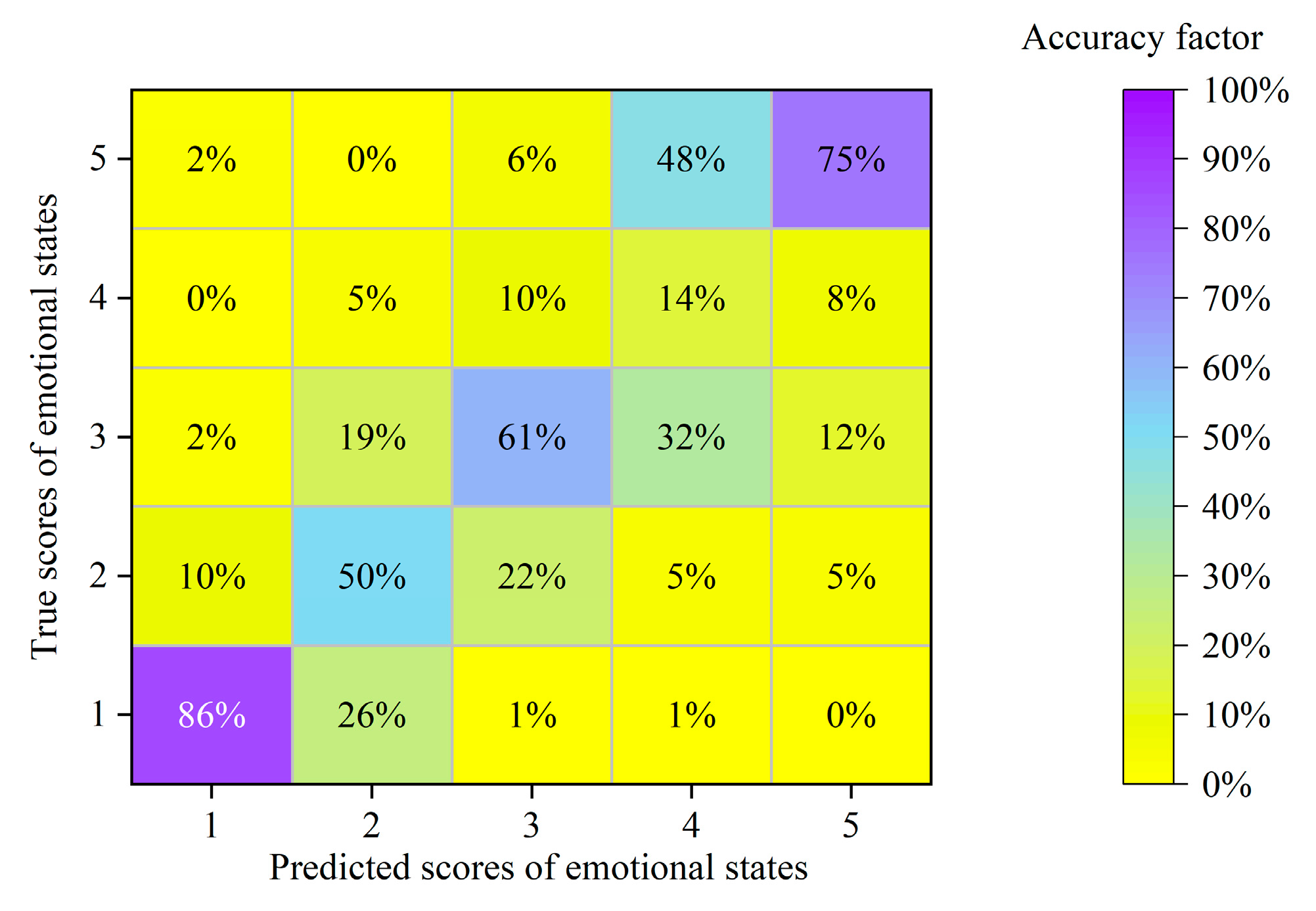
The high prediction accuracy for the very calm state is due to the fact that it has only two transition directions: maintaining the current status or transitioning into the calm state. This makes it relatively easy to predict. Additionally, the changing trend of the very calm state is relatively fixed, with an overall transition towards a calm state over time. Furthermore, the probability of transitioning from the calm state to the very calm state is low, which also contributes to the high prediction accuracy.

(2)

In the absence of intervention measures, the number of passengers in the very calm state decreases rapidly until it reaches zero. As a result, the model’s prediction accuracy for the very calm state reaches 100% on Day 10.

(3)

The prediction accuracy of the extreme anxiety state remained at around 80%, with some fluctuations. This is because there are three possible transition directions for this state, making it not easy to predict accurately. In another, in the absence of interventions, the extreme anxiety state will gradually dominate. There is a reciprocal change between the extreme anxiety state and the anxiety state, leading to fluctuations in prediction accuracy.

(4)

According to the findings presented in Figure 12 and Figure 13, it is evident that the initial few days exhibit a significantly low prediction accuracy for the calm state, with accuracy levels not surpassing 30%. A significant portion of these misclassifications involves predicting a very calm state when the actual state is a calm state. One possible explanation for this observation is that the RF algorithm possesses an inherent tendency to predict extreme emotional states.

Furthermore, Figure 14 and Figure 15 exhibit a notable improvement in the prediction accuracy for the calm state in the later days, surpassing 90%. Moreover, there is a distinct enhancement in the prediction accuracy for the calm state observed in Figure 14 and Figure 15, particularly in the later days, where it consistently exceeds 90%. This significant advancement can be predominantly attributed to the precipitous reduction in the count of passengers experiencing the calm state as time progresses, eventually converging towards zero.

(5)

The predictive precision of both states, anxious and normal, demonstrates a heightened trend of fluctuation. This phenomenon may be attributed to an enhanced tendency of the underlying transitional dynamics between these two states, resulting in frequent and oscillating transitions.

Table 6 presents a statistical table of algorithm indicators, including accuracy, precision, recall, and the F-measure. From

Table 7. Algorithm performance.

	Accuracy	Precision	Recall	F1-Score
Day3	0.57	0.55	0.57	0.54
Day5	0.56	0.54	0.56	0.54
Day7	0.68	0.67	0.69	0.67
Day10	0.81	0.80	0.81	0.81

, it can be seen that the previously introduced model can effectively capture the characteristics of passenger emotion transmission during the SRtP process.

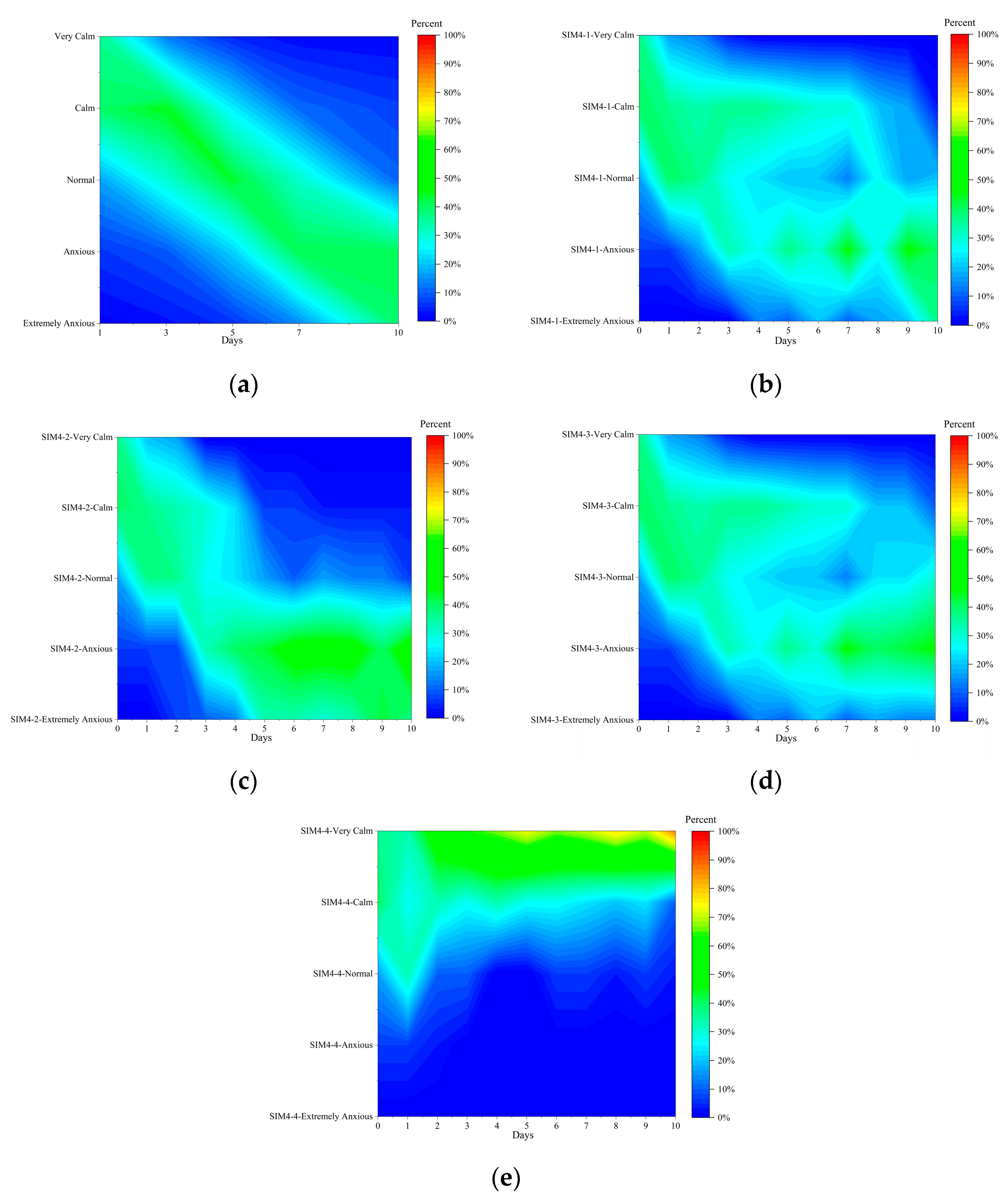
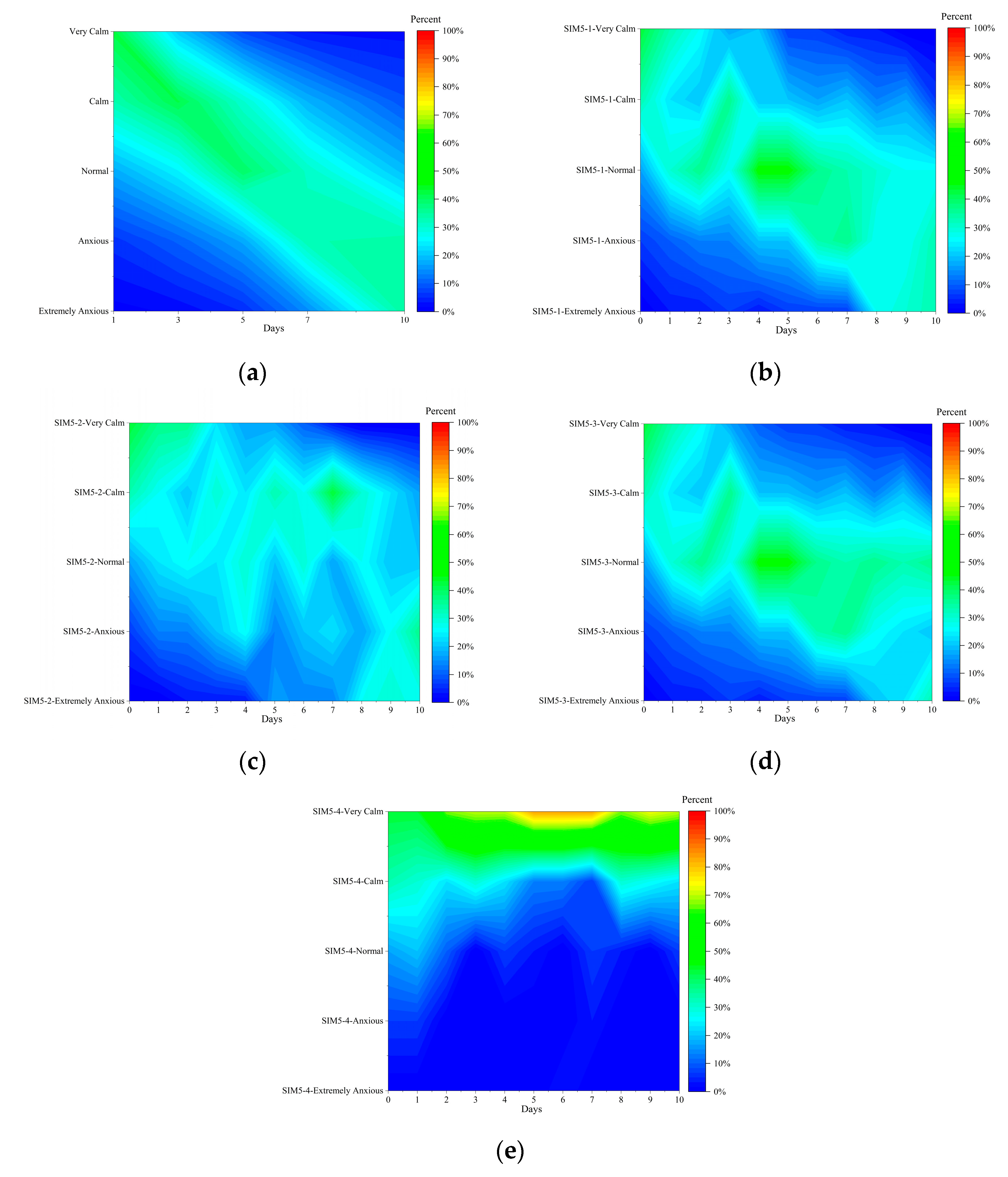
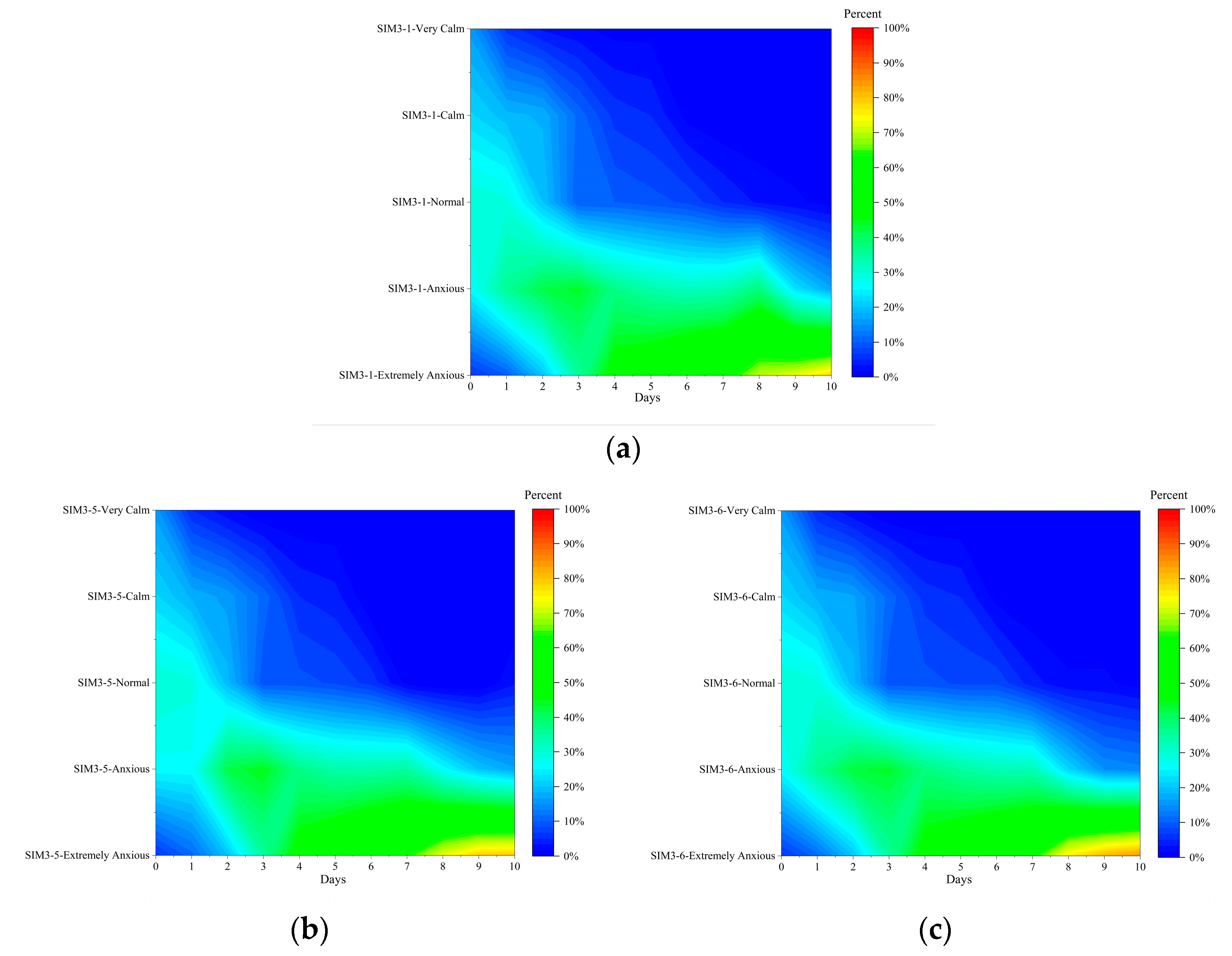
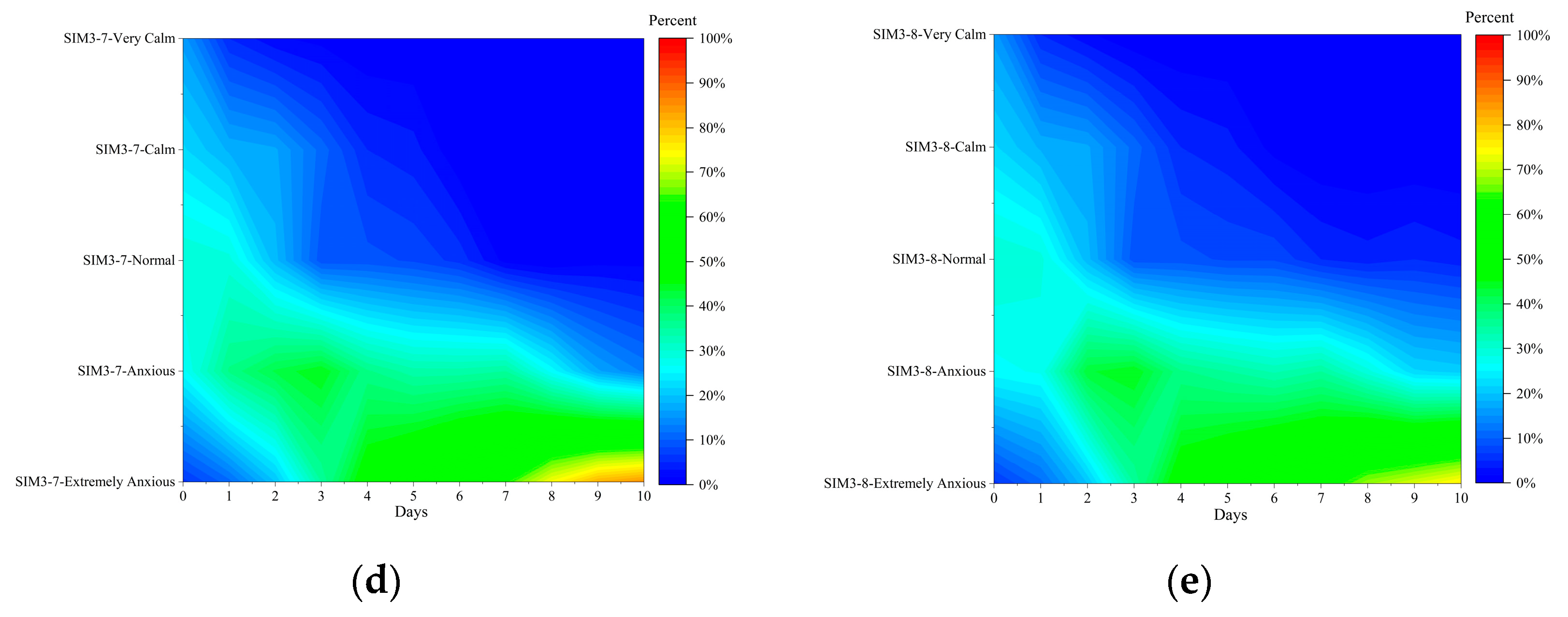
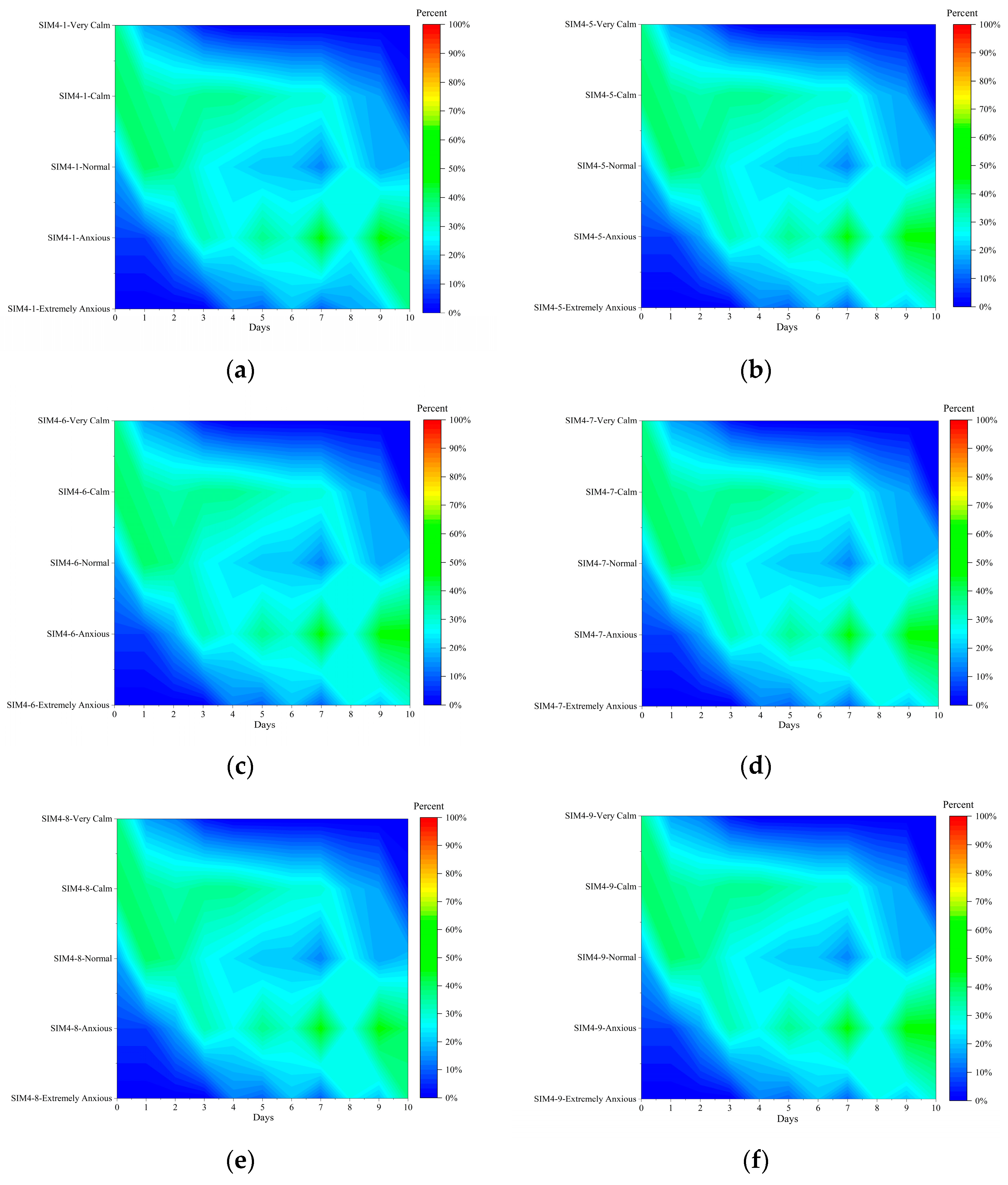
4.3.2. Visualization and Analysis of Emotional Infections in Questionnaire Scenarios

Utilizing the previously introduced model, we simulate and visualize the five scenarios presented in the questionnaire using the AnyLogic software [46]. In order to visualize the process of emotion transmission and examine the variations in its parameters, there are a total of 39 sets of simulation experiments. In Scenario 5, where passengers are equally spaced in front, behind, left, and right, there is no requirement to account for the conversion of spatial grid distribution into rows and columns, unlike the other scenarios.

Table 8. Parameter settings of Scenario 1.

Simulation No.	$({\mathit{a}}_1,{\mathit{b}}_1,{\mathit{a}}_2,{\mathit{b}}_2)$	$\mathbf{Grid} \mathbf{Space} (\mathit{R}\mathit{o}\mathit{w}\times \mathit{C}\mathit{o}\mathit{l}\mathit{u}\mathit{m}\mathit{n})$
$Sim1-1$	$\begin{array}{c}{\mathrm{a}}_1=0.8,{\mathrm{b}}_1=0.8,\\ {\mathrm{a}}_2=0.1,{\mathrm{b}}_2=0.1,\end{array}$	$6\times 5$
$Sim1-2$	$\begin{array}{c}{\mathrm{a}}_1=1,{\mathrm{b}}_1=0,\\ {\mathrm{a}}_2=1,{\mathrm{b}}_2=0,\end{array}$	$6\times 5$
$Sim1-3$	$\begin{array}{c}{\mathrm{a}}_1=0,{\mathrm{b}}_1=1,\\ {\mathrm{a}}_2=0,{\mathrm{b}}_2=1,\end{array}$	$6\times 5$
$Sim1-4$	$\begin{array}{c}{\mathrm{a}}_1=1,{\mathrm{b}}_1=1,\\ {\mathrm{a}}_2=1,{\mathrm{b}}_2=1,\end{array}$	$6\times 5$
$Sim1-5$	$\begin{array}{c}{\mathrm{a}}_1=0.8,{\mathrm{b}}_1=0.8,\\ {\mathrm{a}}_2=0.1,{\mathrm{b}}_2=0.1\end{array}$	$5\times 6$
$Sim1-6$	$\begin{array}{c}{\mathrm{a}}_1=0.8,{\mathrm{b}}_1=0.8,\\ {\mathrm{a}}_2=0.1,{\mathrm{b}}_2=0.1\end{array}$	$3\times 10$
$Sim1-7$	$\begin{array}{c}{\mathrm{a}}_1=0.8,{\mathrm{b}}_1=0.8,\\ {\mathrm{a}}_2=0.1,{\mathrm{b}}_2=0.1\end{array}$	$10\times 3$
$Sim1-8$	$\begin{array}{c}{\mathrm{a}}_1=0.8,{\mathrm{b}}_1=0.8,\\ {\mathrm{a}}_2=0.1,{\mathrm{b}}_2=0.1\end{array}$	$2\times 15$
$Sim1-9$	$\begin{array}{c}{\mathrm{a}}_1=0.8,{\mathrm{b}}_1=0.8,\\ {\mathrm{a}}_2=0.1,{\mathrm{b}}_2=0.1\end{array}$	$15\times 2$

,

Table 9. Parameter settings of Scenario 2.

Simulation No.	$({\mathit{a}}_1,{\mathit{b}}_1,{\mathit{a}}_2,{\mathit{b}}_2)$	$\mathbf{Grid} \mathbf{Space} (\mathit{R}\mathit{o}\mathit{w}\times \mathit{C}\mathit{o}\mathit{l}\mathit{u}\mathit{m}\mathit{n})$
$Sim2-1$	$$\begin{gathered} {\mathrm{a}}_1=0.5,{\mathrm{b}}_1=0.6, \\ {\mathrm{a}}_2=0.2,{\mathrm{b}}_2=0.2, \end{gathered}$$	$8\times 7$ (The space is not fully occupied)
$Sim2-2$	$$\begin{gathered} {\mathrm{a}}_1=1,{\mathrm{b}}_1=0, \\ {\mathrm{a}}_2=1,{\mathrm{b}}_2=0, \end{gathered}$$	$8\times 7$ (The space is not fully occupied)
$Sim2-3$	$$\begin{gathered} {\mathrm{a}}_1=0,{\mathrm{b}}_1=1, \\ {\mathrm{a}}_2=0,{\mathrm{b}}_2=1, \end{gathered}$$	$8\times 7$ (The space is not fully occupied)
$Sim2-4$	$$\begin{gathered} {\mathrm{a}}_1=1,{\mathrm{b}}_1=1, \\ {\mathrm{a}}_2=1,{\mathrm{b}}_2=1, \end{gathered}$$	$8\times 7$ (The space is not fully occupied)
$Sim2-5$	$$\begin{gathered} {\mathrm{a}}_1=0.5,{\mathrm{b}}_1=0.6, \\ {\mathrm{a}}_2=0.2,{\mathrm{b}}_2=0.2, \end{gathered}$$	$8\times 7$ (The space is not fully occupied)
$Sim2-6$	$$\begin{gathered} {\mathrm{a}}_1=0.5,{\mathrm{b}}_1=0.6, \\ {\mathrm{a}}_2=0.2,{\mathrm{b}}_2=0.2, \end{gathered}$$	$5\times 10$
$Sim2-7$	$$\begin{gathered} {\mathrm{a}}_1=0.5,{\mathrm{b}}_1=0.6, \\ {\mathrm{a}}_2=0.2,{\mathrm{b}}_2=0.2, \end{gathered}$$	$10\times 5$
$Sim2-8$	$$\begin{gathered} {\mathrm{a}}_1=0.5,{\mathrm{b}}_1=0.6, \\ {\mathrm{a}}_2=0.2,{\mathrm{b}}_2=0.2, \end{gathered}$$	$2\times 25$

,

Table 10. Parameter settings of Scenario 3.

Simulation No.	$({\mathbf{a}}_1,{\mathbf{b}}_1,{\mathbf{a}}_2,{\mathbf{b}}_2)$	$\mathbf{Grid} \mathbf{Space} (\mathbf{R}\mathbf{o}\mathbf{w}\times \mathbf{C}\mathbf{o}\mathbf{l}\mathbf{u}\mathbf{m}\mathbf{n})$
$Sim3-1$	$$\begin{gathered} {\mathrm{a}}_1=0.2,{\mathrm{b}}_1=0.2, \\ {\mathrm{a}}_2=0.1,{\mathrm{b}}_2=0.1, \end{gathered}$$	$10\times 10$
$Sim3-2$	$$\begin{gathered} {\mathrm{a}}_1=1,{\mathrm{b}}_1=0, \\ {\mathrm{a}}_2=1,{\mathrm{b}}_2=0, \end{gathered}$$	$10\times 10$
$Sim3-3$	$$\begin{gathered} {\mathrm{a}}_1=0,{\mathrm{b}}_1=1, \\ {\mathrm{a}}_2=0,{\mathrm{b}}_2=1, \end{gathered}$$	$10\times 10$
$Sim3-4$	$$\begin{gathered} {\mathrm{a}}_1=1,{\mathrm{b}}_1=1, \\ {\mathrm{a}}_2=1,{\mathrm{b}}_2=1, \end{gathered}$$	$10\times 10$
$Sim3-5$	$$\begin{gathered} {\mathrm{a}}_1=0.2,{\mathrm{b}}_1=0.2, \\ {\mathrm{a}}_2=0.1,{\mathrm{b}}_2=0.1, \end{gathered}$$	$5\times 20$
$Sim3-6$	$$\begin{gathered} {\mathrm{a}}_1=0.2,{\mathrm{b}}_1=0.2, \\ {\mathrm{a}}_2=0.1,{\mathrm{b}}_2=0.1, \end{gathered}$$	$20\times 5$
$Sim3-7$	$$\begin{gathered} {\mathrm{a}}_1=0.2,{\mathrm{b}}_1=0.2, \\ {\mathrm{a}}_2=0.1,{\mathrm{b}}_2=0.1, \end{gathered}$$	$4\times 25$
$Sim3-8$	$$\begin{gathered} {\mathrm{a}}_1=0.2,{\mathrm{b}}_1=0.2, \\ {\mathrm{a}}_2=0.1,{\mathrm{b}}_2=0.1, \end{gathered}$$	$25\times 4$

,

Table 11. Parameter settings of Scenario 4.

Simulation No.	$({\mathbf{a}}_1,{\mathbf{b}}_1,{\mathbf{a}}_2,{\mathbf{b}}_2)$	$\mathbf{Grid} \mathbf{Space} (\mathbf{R}\mathbf{o}\mathbf{w}\times \mathbf{C}\mathbf{o}\mathbf{l}\mathbf{u}\mathbf{m}\mathbf{n})$
$Sim4-1$	$$\begin{gathered} {\mathrm{a}}_1=0.3,{\mathrm{b}}_1=0.3, \\ {\mathrm{a}}_2=0.1,{\mathrm{b}}_2=0.1, \end{gathered}$$	$6\times 5$
$Sim4-2$	$$\begin{gathered} {\mathrm{a}}_1=1,{\mathrm{b}}_1=0, \\ {\mathrm{a}}_2=1,{\mathrm{b}}_2=0, \end{gathered}$$	$6\times 5$
$Sim4-3$	$$\begin{gathered} {\mathrm{a}}_1=0,{\mathrm{b}}_1=1, \\ {\mathrm{a}}_2=0,{\mathrm{b}}_2=1, \end{gathered}$$	$6\times 5$
$Sim4-4$	$$\begin{gathered} {\mathrm{a}}_1=1,{\mathrm{b}}_1=1, \\ {\mathrm{a}}_2=1,{\mathrm{b}}_2=1, \end{gathered}$$	$6\times 5$
$Sim4-5$	$$\begin{gathered} {\mathrm{a}}_1=0.3,{\mathrm{b}}_1=0.3, \\ {\mathrm{a}}_2=0.1,{\mathrm{b}}_2=0.1 \end{gathered}$$	$5\times 6$
$Sim4-6$	$$\begin{gathered} {\mathrm{a}}_1=0.3,{\mathrm{b}}_1=0.3, \\ {\mathrm{a}}_2=0.1,{\mathrm{b}}_2=0.1 \end{gathered}$$	$3\times 10$
$Sim4-7$	$$\begin{gathered} {\mathrm{a}}_1=0.3,{\mathrm{b}}_1=0.3, \\ {\mathrm{a}}_2=0.1,{\mathrm{b}}_2=0.1 \end{gathered}$$	$10\times 3$
$Sim4-8$	$$\begin{gathered} {\mathrm{a}}_1=0.3,{\mathrm{b}}_1=0.3, \\ {\mathrm{a}}_2=0.1,{\mathrm{b}}_2=0.1 \end{gathered}$$	$2\times 15$
$Sim4-9$	$$\begin{gathered} {\mathrm{a}}_1=0.3,{\mathrm{b}}_1=0.3, \\ {\mathrm{a}}_2=0.1,{\mathrm{b}}_2=0.1 \end{gathered}$$	$15\times 2$

and

Table 12. Parameter settings of Scenario 5.

Simulation No.	$({\mathbf{a}}_1,{\mathbf{b}}_1,{\mathbf{a}}_2,{\mathbf{b}}_2)$	$\mathbf{Grid} \mathbf{Space} (\mathbf{R}\mathbf{o}\mathbf{w}\times \mathbf{C}\mathbf{o}\mathbf{l}\mathbf{u}\mathbf{m}\mathbf{n})$
$Sim5-1$	$$\begin{gathered} {\mathrm{a}}_1=0.3,{\mathrm{b}}_1=0.3, \\ {\mathrm{a}}_2=0.1,{\mathrm{b}}_2=0.1, \end{gathered}$$	$6\times 5$
$Sim5-2$	$$\begin{gathered} {\mathrm{a}}_1=1,{\mathrm{b}}_1=0, \\ {\mathrm{a}}_2=1,{\mathrm{b}}_2=0, \end{gathered}$$	$6\times 5$
$Sim5-3$	$$\begin{gathered} {\mathrm{a}}_1=0,{\mathrm{b}}_1=1, \\ {\mathrm{a}}_2=0,{\mathrm{b}}_2=1, \end{gathered}$$	$6\times 5$
$Sim5-4$	$$\begin{gathered} {\mathrm{a}}_1=1,{\mathrm{b}}_1=1, \\ {\mathrm{a}}_2=1,{\mathrm{b}}_2=1, \end{gathered}$$	$6\times 5$
$Sim5-5$	$$\begin{gathered} {\mathrm{a}}_1=0.3,{\mathrm{b}}_1=0.3, \\ {\mathrm{a}}_2=0.1,{\mathrm{b}}_2=0.1 \end{gathered}$$	$3\times 10$
$Sim5-6$	$$\begin{gathered} {\mathrm{a}}_1=0.3,{\mathrm{b}}_1=0.3, \\ {\mathrm{a}}_2=0.1,{\mathrm{b}}_2=0.1 \end{gathered}$$	$2\times 15$

show the parameter settings for each simulation experiment for Scenarios 1 to 5. The value of $(a_1, b_1, a_2, b_2)$ can be adjusted through machine learning techniques, where the value of $(a_1, b_1, a_2, b_2)$ for $(Sim1-1, Sim2-1, Sim3-1, Sim4-1, Sim5-1)$ are obtained through manual tuning. Grid space is the hyperparameter of this model. We examine how hyperparameters affect the model by configuring various grid spaces such as $(Sim1-1, Sim1-5 to 9$).

Figure 16, Figure 17, Figure 18, Figure 19 and Figure 20 provide a depiction of how the trend in passenger emotions evolves with varying values of the parameters $(a_1, b_1, a_2, b_2)$. The x-axis in these figures represents the number of days, while the y-axis illustrates the proportions of passengers in different emotional states. These figures make it readily apparent how different emotional states change over time and highlight the disparities in emotional state proportions within each day. Furthermore, these figures offer a clear and intuitive representation of the fluctuations in passenger emotional states.

Figure 16 presents the distribution of different emotional states among passengers in Scenario 1 for different values of the parameter $(a_1, b_1, a_2, b_2)$. When comparing Figure 16c–e, we observe that, despite the identical coefficients for $R\left(E\right)$ and $R\left(V\right)$ in these three graphs, there are notable distinctions in the distribution of passenger proportions. In Figure 16c, although the overall distribution closely aligns with the original data, there is a noticeable increase in fluctuation trends. Figure 16d exhibits even more pronounced fluctuation trends, while the distribution in Figure 16e differs substantially from the original data. By contrasting the values of parameter $(a_1, b_1, a_2, b_2)$ in these graphs, we can deduce that in Scenario 1, time exerts a predominant influence in comparison to the inter-individual distances within the population.

Figure 17 illustrates the distribution of passengers in various emotional states in Scenario 2, under different values of the parameter $(a_1, b_1, a_2, b_2)$. Similarly, when comparing Figure 17c–e, it is evident that they closely resemble the trends observed in the original data. Figure 17c,e seem to project potential future states of the original data, with e exhibiting a notably accelerated rate of development. In contrast, Figure 17d demonstrates more significant fluctuations compared to the original dataset. By examining the values of parameter $(a_1, b_1, a_2, b_2)$ in these graphs, it becomes evident that in Scenario 2, the impact of time is considerably more pronounced.

With the continual expansion of the passenger population, the impact of time becomes notably more significant, as clearly evident in Figure 18c,e. Interestingly, when comparing Figure 18c–e, it becomes apparent that the fluctuations are gradually decreasing. One possible explanation for this trend is that as the total number of passengers increases, there is a directed influence causing passenger emotions to shift towards anxiety.

Comparing Figure 16 and Figure 19 both horizontally and vertically reveals a notable trend: as the distance between passengers increases, the influence of distance decreases significantly. Additionally, there is a consistent shift toward calmer emotional states among passengers overall. When we contrast Scenario 1 with Scenario 4, a few key observations emerge. In Scenario 4, the proportion of passengers experiencing extreme anxiety further decreases, while the proportion of those in very calm and calm emotional states rises. This highlights a significant shift towards emotional calmness in Scenario 4 as compared to Scenario 1.

Upon a comprehensive comparison of Figure 16, Figure 19 and Figure 20, a significant trend becomes evident: as the distance between passengers increases, it intensifies the fluctuations among several positive emotional states. Additionally, this widening distance leads to a further reduction in the proportion of passengers experiencing extreme anxiety.

Based on the patterns analyzed earlier, an attempt is made to manually fine-tune the parameters, as shown in the $\left(\mathrm{b}\right)$ subfigures in Figure 16, Figure 17, Figure 18, Figure 19 and Figure 20. Further statistical analysis was conducted to assess the tuning results. Figure 21, Figure 22, Figure 23, Figure 24 and Figure 25 illustrate the difference-values (D-value) in emotional state distributions corresponding to different parameters over time, while

Table 13. Descriptive Statistics of Extremely Anxious.

	Mean	Standard Deviation	Mean SE	Sum	Harmonic Mean	Minimum	Maximum
Extremely Anxious	0.16948	0.23723	0.10609	0.8474	0.02103	0.0094	0.5687
SIM1-1-Extremely Anxious	0.17333	0.22534	0.10077	0.86667	0	0	0.56667
SIM1-2-Extremely Anxious	0.15333	0.10435	0.04667	0.76667	0	0	0.26667
SIM1-3-Extremely Anxious	0.08	0.05055	0.02261	0.4	0	0	0.13333
SIM1-4-Extremely Anxious	0.02	0.01826	0.00816	0.1	0	0	0.03333

,

Table 14. Descriptive Statistics of Anxious.

	Mean	Standard Deviation	Mean SE	Sum	Harmonic Mean	Minimum	Maximum
Anxious	0.24936	0.19171	0.08574	1.2468	0.10677	0.0358	0.5217
SIM1-1-Anxious	0.33333	0.14337	0.06412	1.66667	0.27121	0.13333	0.53333
SIM1-2-Anxious	0.34667	0.21807	0.09752	1.73333	0.25135	0.13333	0.66667
SIM1-3-Anxious	0.34667	0.14644	0.06549	1.73333	0.27815	0.13333	0.5
SIM1-4-Anxious	0.04667	0.05055	0.02261	0.23333	0	0	0.1

,

Table 15. Descriptive Statistics of Normal.

	Mean	Standard Deviation	Mean SE	Sum	Harmonic Mean	Minimum	Maximum
Normal	0.23352	0.13432	0.06007	1.1676	0.17736	0.0998	0.42
SIM1-1-Normal	0.24	0.13208	0.05907	1.2	0.11242	0.03333	0.36667
SIM1-2-Normal	0.2	0.09129	0.04082	1	0.16787	0.1	0.33333
SIM1-3-Normal	0.29333	0.05963	0.02667	1.46667	0.28357	0.23333	0.36667
SIM1-4-Normal	0.13333	0.06667	0.02981	0.66667	0.08772	0.03333	0.2

,

Table 16. Descriptive Statistics of Calm.

	Mean	Standard Deviation	Mean SE	Sum	Harmonic Mean	Minimum	Maximum
Calm	0.2422	0.20458	0.09149	1.211	0.08732	0.0301	0.4765
SIM1-1-Calm	0.2	0.11055	0.04944	1	0.10511	0.03333	0.33333
SIM1-2-Calm	0.22	0.20083	0.08981	1.1	0.07143	0.03333	0.5
SIM1-3-Calm	0.22667	0.06831	0.03055	1.13333	0.21212	0.16667	0.33333
SIM1-4-Calm	0.27333	0.11879	0.05312	1.36667	0.21607	0.1	0.43333

and

Table 17. Descriptive Statistics of Very Calm.

	Mean	Standard Deviation	Mean SE	Sum	Harmonic Mean	Minimum	Maximum
Very Calm	0.10546	0.1628	0.07281	0.5273	0.01622	0.0056	0.3898
SIM1-1-Very Calm	0.05333	0.08367	0.03742	0.26667	0	0	0.2
SIM1-2-Very Calm	0.08	0.14453	0.06464	0.4	0	0	0.33333
SIM1-3-Very Calm	0.05333	0.08367	0.03742	0.26667	0	0	0.2
SIM1-4-Very Calm	0.52667	0.13622	0.06092	2.63333	0.49826	0.36667	0.66667

provide a concise summary of the statistical analysis. Figure 26, Figure 27, Figure 28, Figure 29 and Figure 30 show the simulation results of manual parameter adjustment.

It is evident from the presented charts and tables that the manual parameter tuning yielded highly favorable outcomes. Moreover, during the manual tuning process, it is noted that parameter $(a_1, b_1, a_2, b_2)$ demonstrate closer alignment with the initial data when all its values are less than 1. This observation could be attributed to the fact that the incidents triggering the cruise ship’s execution of the SRtP procedure are not overly severe, resulting in relatively minor effects on emotional transitions. However, as the incident duration increases, the impact accelerates.

The scenario parameters and simulation results are shown in Figure 16, Figure 17, Figure 18, Figure 19, Figure 20, Figure 21, Figure 22, Figure 23, Figure 24 and Figure 25. In the scene simulation diagrams, red indicates extremely anxious passengers, orange indicates generally anxious passengers, green indicates normal passengers, light blue indicates generally calm passengers and purple indicates very calm passengers.

Figure 31, Figure 32, Figure 33, Figure 34 and Figure 35 present an analysis of the impact of spatial grid distribution on emotional transitions based on the results of manual parameter tuning, specifically exploring the influence of model hyperparameters.

In Figure 31, when comparing subfigures horizontally, it becomes evident that the conversion of rows and columns in two different spatial grid configurations affects emotional state transitions. Vertical comparisons, on the other hand, reveal that a complete alteration of the spatial grid distribution may or may not influence emotional state transitions.

A similar trend is observed in Figure 32. In horizontal comparisons, there exists a set of spatial grid row–column conversions that do not produce discernible impacts. In vertical comparisons, instances of a radical shift in grid distribution do not result in corresponding changes in emotional state distributions.

Figure 33 highlights this phenomenon more prominently, with emotional state distributions across all comparison groups undergoing only minimal changes.

Both Figure 34 and Figure 35, whether involving the conversion of rows and columns within the spatial grid or an entire overhaul of the grid, show no notable changes in the distribution of emotional states.

Several factors may contribute to these observations:

• In the model developed in this study, the distance component is relatively minor compared to the temporal component, and its influence diminishes as time progresses.
• The original data and simulations are based on a daily time scale, with no exploration of scenarios where $t$ falls between 0 and 1. According to the proposed model, distance effects become dominant only when $t$ is small.
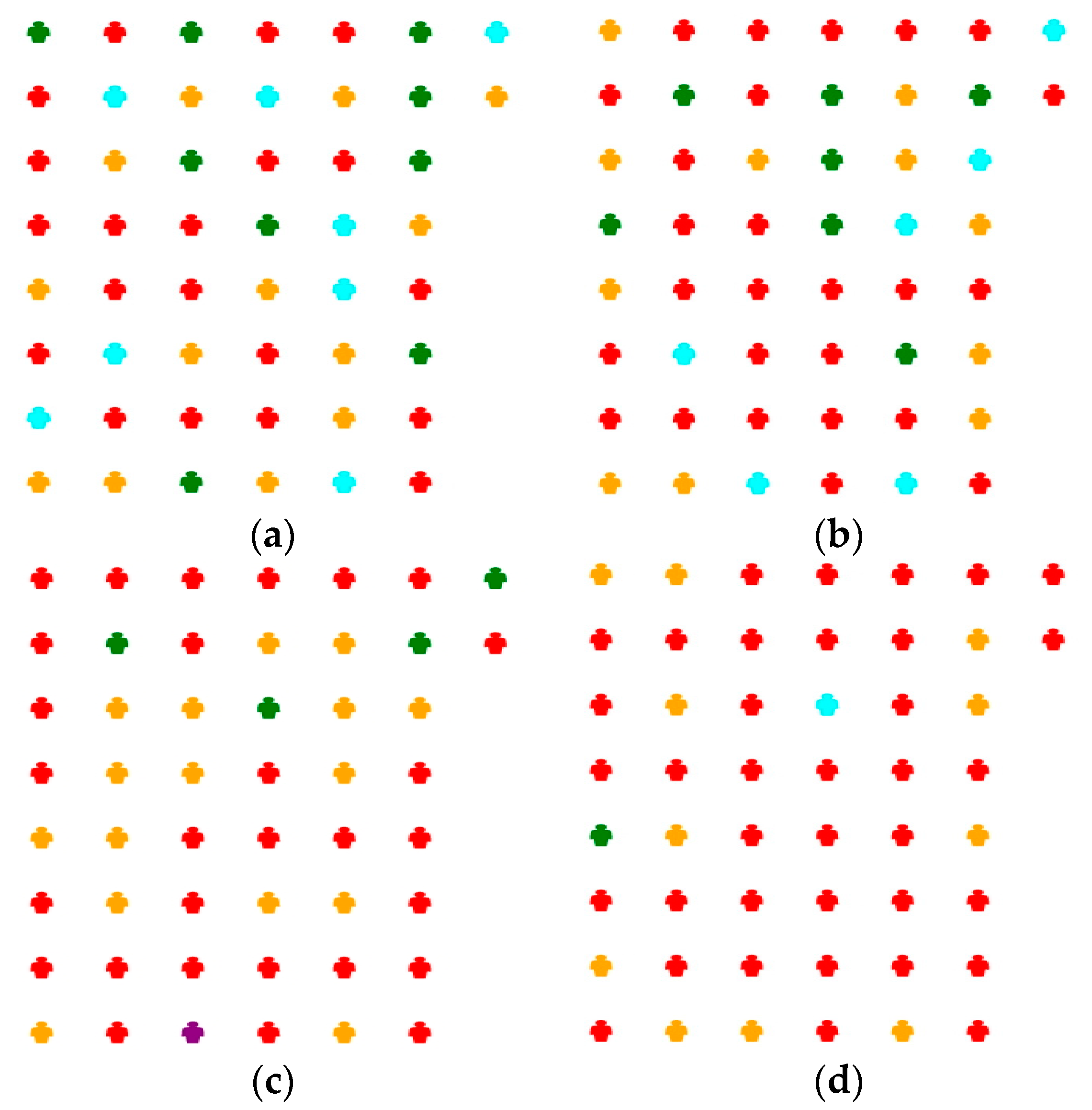
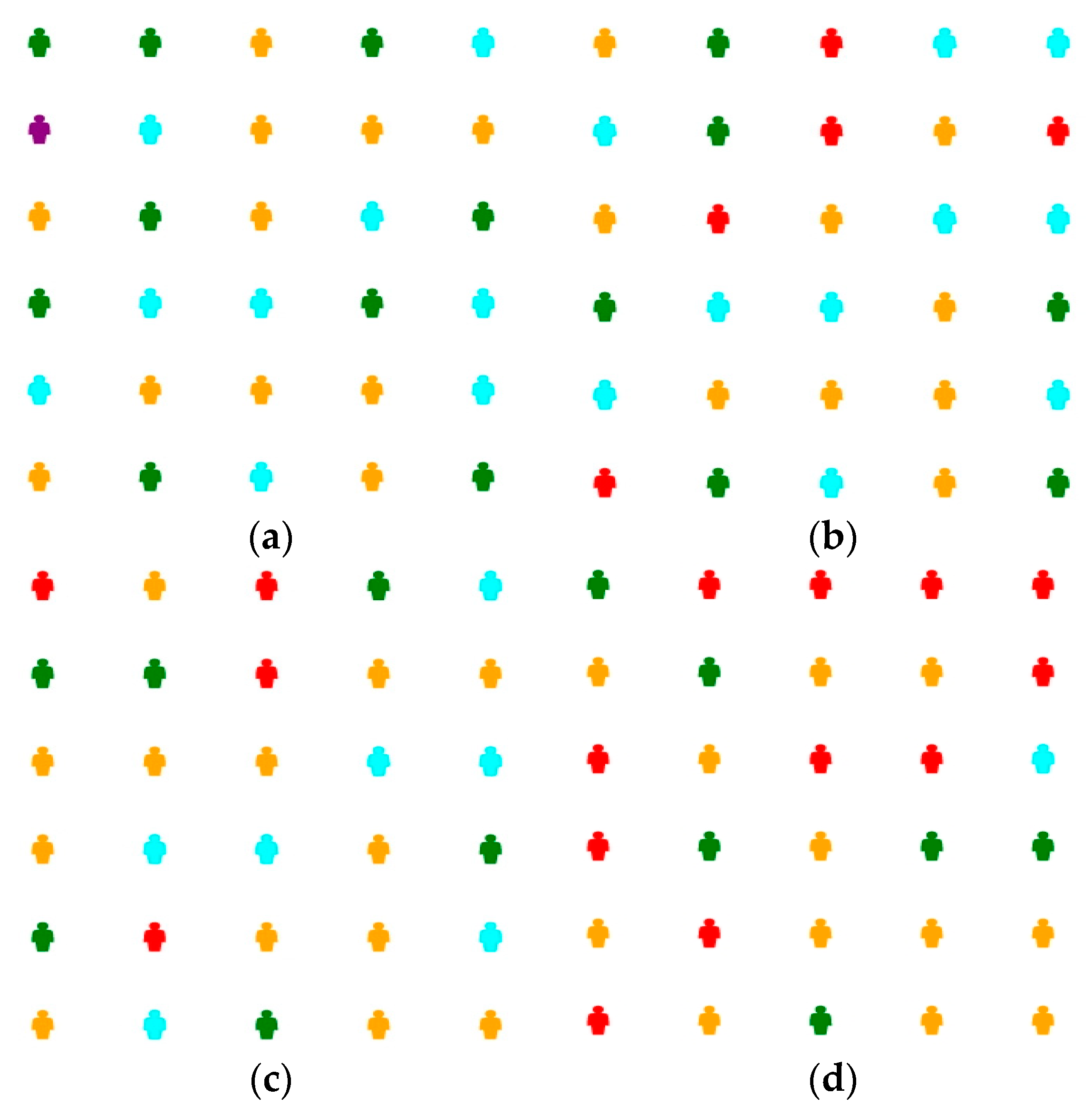
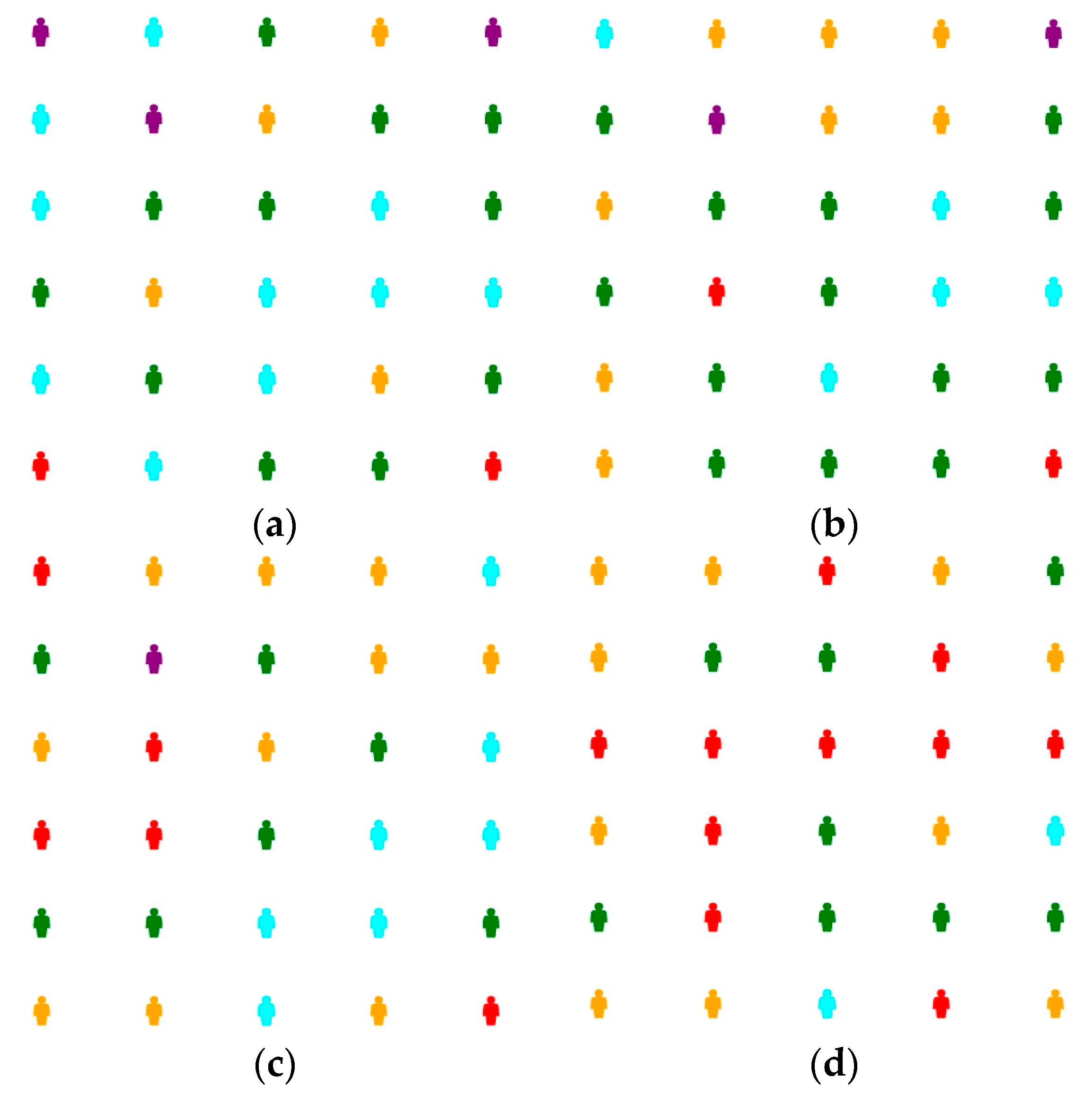
• Emotional transmission emanates from the infection source and radiates outward, potentially affecting eight, five, or three individuals in the first level of transmission. Calculations using Euclidean distance indicate that, when conducting row–column conversions within spatial grids, the overall dynamics of the first-level transmission remain unaltered. However, the impact gradually becomes noticeable in the second-level transmission. Notably, the magnitude of this effect increases with greater disparities in row and column distances within the spatial grid.

The aforementioned observations indicate that, in prolonged shelter-in-place scenarios akin to SRtP, the spatial distribution of individuals exerts a minimal influence on the overall emotional state transitions. This implies that safety planning for such scenarios can incorporate more flexible designs for the shape of spaces.

Upon comparing Figure 31, Figure 32 and Figure 33, it becomes apparent that, as the total number of passengers increases, altering the spatial grid distribution does not significantly reduce the likelihood of emotional transitions towards anxiety. However, strategically implementing spatial separation to reduce the total number of individuals in each space can indeed diminish this probability.

Further comparisons involving Figure 31, Figure 34 and Figure 35 reveal that appropriately increasing the distance between individuals does contribute to a lower overall likelihood of emotional transitions towards anxiety.

5. Conclusions and Future Work

This study is centered on the emotional contagion process during the cruise ship SRtP (Ship-to-Rescue-Platform) procedure and presents an improved SIR (Susceptible-Infection-Removal) model. In comparison to other emotional contagion models, the one proposed in this paper expands its scope across emotional state divisions, contagion source configurations, and transition directions. By combining it with the weighted random forest algorithm for emotional state distribution prediction, the results demonstrate that this model adeptly captures the fluctuating characteristics inherent in the emotional transition process. Through simulation experiments, we visualize these fluctuating characteristics during emotional transition, employing multiple control groups with varying parameters to analyze the effects of parameter variations.

Although this research focuses on a specific passenger group, the proposed model exhibits applicability to similar extended-duration emergency scenarios. In summary, the research findings explore and substantiate the efficacy of the enhanced SIR model in modeling the emotional contagion process among passengers during the cruise ship SRtP procedure.

In future research endeavors, we contemplate the integration of individual traits and demographic factors for further model refinement.

References

1. International Maritime Organization. SOLAS: The International Convention for the Safety of Life at Sea; International Maritime Organization: London, UK, 2020. [Google Scholar]
2. Tripathi, G.; Singh, K.; Vishwakarma, D.K. Crowd Emotion Analysis Using 2D ConvNets. In Proceedings of the 2020 Third International Conference on Smart Systems and Inventive Technology (ICSSIT), Tirunelveli, India, 20–22 August 2020. [Google Scholar]
3. Varghese, E.B.; Thampi, S.M. A Deep Learning Approach to Predict Crowd Behavior Based on Emotion. In Smart Multimedia; Indian Institute of Information Technology and Management-Kerala (IIITM-K): Thiruvananthapuram, India; Cochin University of Science and Technology: Kochi, India, 2018. [Google Scholar]
4. Sanchez, F.L. Revisiting crowd behaviour analysis through deep learning: Taxonomy, anomaly detection, crowd emotions, datasets, opportunities and prospects. Inf. Fusion 2020, 64, 318–335. [Google Scholar] [CrossRef] [PubMed]
5. Varghese, E.; Thampi, S.M.; Berretti, S. A Psychologically Inspired Fuzzy Cognitive Deep Learning Framework to Predict Crowd Behavior. IEEE Trans. Affect. Comput. 2020, 13, 1005–1022. [Google Scholar] [CrossRef]
6. Singh, N.; Roy, N.; Gangopadhyay, A. Analyzing the Emotions of Crowd for Improving the Emergency Response Services. Pervasive Mob. Comput. 2019, 58, 101018. [Google Scholar] [CrossRef]
7. Watanabe, K.; Inoue, K. Learning State Transition Rules from High-Dimensional Time Series Data with Recurrent Temporal Gaussian-Bernoulli Restricted Boltzmann Machines. Hum.-Centric Intell. Syst. 2023, 3, 296–311. [Google Scholar] [CrossRef]
8. Amato, F.; Guignard, F.; Robert, S.; Kanevski, M. A novel framework for spatio-temporal prediction of environmental data using deep learning. Sci. Rep. 2020, 10, 22243. [Google Scholar] [CrossRef]
9. Xu, Y.; Tian, Y.; Li, H. Unsupervised deep learning method for bridge condition assessment based on intra-and inter-class probabilistic correlations of quasi-static responses. Struct. Health Monit. 2023, 22, 600–620. [Google Scholar] [CrossRef]
10. Tian, Y.; Xu, Y.; Zhang, D.; Li, H. Relationship modeling between vehicle-induced girder vertical deflection and cable tension by BiLSTM using field monitoring data of a cable-stayed bridge. Struct. Control Health Monit. 2021, 28, e2667. [Google Scholar] [CrossRef]
11. Lv, P.; Xu, B.; Li, C.; Yu, Q.; Zhou, B.; Xu, M. Antagonistic Crowd Simulation Model Integrating Emotion Contagion and Deep Reinforcement Learning. arXiv 2021, arXiv:2015.00854. [Google Scholar] [CrossRef]
12. Xue, J.; Yin, H.; Lv, P.; Xu, M.; Li, Y. Crowd queuing simulation with an improved emotional contagion model. Sci. China 2019, 62, 193–195. [Google Scholar] [CrossRef]
13. Rao, M.Y. Crowd evacuation simulation based on emotion contagion. Int. J. Simul. Process Model. 2018, 13, 43–56. [Google Scholar] [CrossRef]
14. Xu, T.; Shi, D.; Chen, J.; Li, T.; Lin, P.; Ma, J. Dynamics of emotional contagion in dense pedestrian crowds. Phys. Lett. A 2019, 384, 126080. [Google Scholar] [CrossRef]
15. Shi, Y.; Zhang, G.; Lu, D.; Lv, L.; Liu, H. Adaptive Intervention for Crowd Negative Emotional Contagion. In Proceedings of the 2021 IEEE 24th International Conference on Computer Supported Cooperative Work in Design (CSCWD), Dalian, China, 5–7 May 2021; IEEE: Washington, DC, USA, 2021. [Google Scholar]
16. Hethcote, H.W. The mathematics of infectious diseases. SIAM Rev. 2000, 42, 99–653. [Google Scholar] [CrossRef]
17. Bairagi, N.; Adak, D. Global analysis of hiv-1 dynamics with hill type infection rate and intracellular delay. Appl. Math. Model. 2014, 38, 5047–5066. [Google Scholar] [CrossRef]
18. Feng, L.; Liao, X.; Han, Q.; Li, H. Dynamical analysis and control strategies on malware propagation model. Appl. Math. Model. 2013, 37, 8225–8236. [Google Scholar] [CrossRef]
19. Ji, C.; Jiang, D. Threshold behavior of a stochastic sir model. Appl. Math. Model. 2014, 38, 5067–5079. [Google Scholar] [CrossRef]
20. Liu, H.; Lu, D.; Zhang, G.; Hong, X.; Liu, H. Recurrent emotional contagion for the crowd evacuation of a cyber-physical society. Inf. Sci. 2021, 10, 155–172. [Google Scholar] [CrossRef]
21. Qiu, L.; Liu, S. SVIR rumor spreading model considering individual vigilance awareness and emotion in social networks. Int. J. Mod. Phys. C 2021, 32, 2150120. [Google Scholar] [CrossRef]
22. Chen, Y.H.; Zhang, X.Q. Research on Netizen Group Emotion Contagion Model and the Simulation under Network Group Emergencies. Inf. Sci. 2018, 36, 151–156. [Google Scholar] [CrossRef]
23. Nizamani, S.; Memon, N.; Galam, S. From public outrage to the burst of public violence: An epidemic-like model. Phys. A Stat. Mech. Appl. 2014, 416, 620–630. [Google Scholar] [CrossRef]
24. Zhu, L.; Wang, B. Stability analysis of a SAIR rumor spreading model with control strategies in online social networks. Inf. Sci. 2020, 526, 1–19. [Google Scholar] [CrossRef]
25. Tian, S.H.; Sun, M.Q.; Zhang, J.Y. Research on the Emotion Evolution of Network Public Opinion Based on Improved SIR Model. Inf. Sci. 2019, 37, 52–57,64. [Google Scholar] [CrossRef]
26. Xu, M.; Li, C.; Lv, P.; Chen, W.; Deng, Z.; Zhou, B.; Manocha, D. Emotion-based crowd simulation model based on physical strength consumption for emergency scenarios. IEEE Trans. Intell. Transp. Syst. 2020, 22, 6977–6991. [Google Scholar] [CrossRef]
27. Song, J.; Zhang, M.G. Dynamic Simulation of the Group Behavior under Fire Accidents Based on System Dynamics. Procedia Eng. 2018, 211, 635–643. [Google Scholar] [CrossRef]
28. Song, B.W.; Li, J.; Li, J. Considering Trust Parameters the Evolution Model of Network Negative Emotion under Public Emergencies. In Proceedings of the 2020 4th International Conference on Electronic Information Technology and Computer Engineering, Xiamen, China, 6–8 November 2020. [Google Scholar]
29. Yao, J.J.; Liang, J.; Yao, H.X. Research on Emotional Information Communication Based on SIR Model. Inf. Sci. 2018, 36, 25–29. [Google Scholar] [CrossRef]
30. Cao, M.; Zhang, G.; Wang, M.; Lu, D.; Liu, H. A method of emotion contagion for crowd evacuation. Phys. A Stat. Mech. Appl. 2017, 483, 250–258. [Google Scholar] [CrossRef]
31. Fan, R.; Xu, K.; Zhao, J. An agent-based model for emotion contagion and competition in online social media. Phys. A Stat. Mech. Appl. 2017, 495, 245–259. [Google Scholar] [CrossRef]
32. Li, X.; Zhang, J. Research on SIRS Information Dissemination Model Based on System Dynamics. Inf. Sci. 2017, 35, 17–22. [Google Scholar] [CrossRef]
33. Hatfield, E.; Cacioppo, J.T.; Rapson, R.L. Emotional Contagion. Curr. Dir. Psychol. Sci. 1993, 2, 96–100. [Google Scholar] [CrossRef]
34. Shi, Y.; Zhang, G.; Lu, D.; Lv, L.; Liu, H. Intervention Optimization for Crowd Emotional Contagion. Inf. Sci. 2021, 576, 769–789. [Google Scholar] [CrossRef]
35. Guttman, L. A basis for analyzing test-retest reliability. Psychometrika 1945, 10, 255–282. [Google Scholar] [CrossRef]
36. Lopez-Odar, D.; Alvarez-Risco, A.; Vara-Horna, A.; Chafloque-Cespedes, R.; Sekar, M.C. Validity and reliability of the questionnaire that evaluates factors associated with perceived environmental behavior and perceived ecological purchasing behavior in Peruvian consumers. Soc. Responsib. J. 2020, 16, 403–417. [Google Scholar] [CrossRef]
37. Chung, R.H.; Kim, B.S.; Abreu, J.M. Asian American multidimensional acculturation scale: Development, factor analysis, reliability, and validity. Cult. Divers. Ethn. Minor Psychol. 2004, 10, 66–80. [Google Scholar] [CrossRef] [PubMed]
38. Elliott, A.C.; Hynan, L.S. A SAS(R) macro implementation of a multiple comparison post hoc test for a Kruskal-Wallis analysis. Comput. Methods Programs Biomed. 2011, 102, 75–80. [Google Scholar] [CrossRef] [PubMed]
39. Breiman, L. Random forests. Mach. Learn. 2001, 45, 5–32. [Google Scholar] [CrossRef]
40. Goel, S.; Watts, D.J.; Goldstein, D.G. The Structure of Online Diffusion Networks. In Proceedings of the 13th ACM Conference on Electronic Commerce, Valencia, Spain, 4–8 June 2012. [Google Scholar]
41. Hu, C.; Chen, Y.; Hu, L.; Peng, X. A novel random forests based class incremental learning method for activity recognition. Pattern Recognit. 2018, 78, 277–290. [Google Scholar] [CrossRef]
42. Abell’an, J.; Mantas, C.J.; Castellano, J.G.; Moral-García, S. Increasing diversity in random forest learning algorithm via imprecise probabilities. Expert Syst. Appl. 2018, 97, 228–243. [Google Scholar] [CrossRef]
43. Gomes, H.M.; Bifet, A.; Read, J.; Barddal, J.P.; Enembreck, F.; Pfharinger, B.; Holmes, G.; Abdessalem, T. Adaptive ra-ndom forests for evolving data stream classification. Mach. Learn. 2017, 106, 1469–1495. [Google Scholar] [CrossRef]
44. Genuer, R.; Poggi, J.; Tuleau-Malot, C.; Villa-Vialaneix, N. Random forests for big data. Big Data Res. 2017, 9, 28–46. [Google Scholar] [CrossRef]
45. Zhu, M.; Xia, J.; Jin, X.; Yan, M.; Cai, G.; Yan, J.; Ning, G. Class weights random forest algorithm for processing class imbalanced medical data. IEEE Access 2018, 6, 4641–4652. [Google Scholar] [CrossRef]
46. Anylogic. Available online: https://www.anylogic.com// (accessed on 15 February 2023).
Figure 1. Relationship between emotional state transitions ( α i j is the probability of transition from state i to state j ).
Mathematics 11 04461 g001
Figure 2. Distribution of public space selection.
Mathematics 11 04461 g002
Figure 3. Emotional state distribution in Scenario 1 (   ρ = 2   m 2 / p e r s o n , n = 30 ).
Mathematics 11 04461 g003
Figure 4. Emotional state distribution in Scenario 2 (   ρ = 2   m 2 / p e r s o n , n = 50 ).
Mathematics 11 04461 g004
Figure 5. Emotional state distribution in Scenario 3 (   ρ = 2   m 2 / p e r s o n , n = 100 ).
Mathematics 11 04461 g005
Figure 6. Emotional state distribution in Scenario 4 (   ρ = 3   m 2 / p e r s o n , n = 30 ).
Mathematics 11 04461 g006
Figure 7. Emotional State Distribution in SCENARIO 5 (   ρ = 4   m 2 / p e r s o n , n = 30 ).
Mathematics 11 04461 g007
Figure 8. Box chart of daily emotional states at different population densities.
Mathematics 11 04461 g008
Figure 9. Box chart of emotional states of different total passengers.
Mathematics 11 04461 g009
Figure 10. The population space; (a) 2   m 2 / p e r s o n ; (b) 3   m 2 / p e r s o n ; (c) 4   m 2 / p e r s o n .
Mathematics 11 04461 g010
Figure 11. The algorithm flowchart.
Mathematics 11 04461 g011
Figure 12. Confusion matrix of forecast results for Day 3.
Mathematics 11 04461 g012
Figure 13. Confusion matrix of forecast results for Day 5.
Mathematics 11 04461 g013
Figure 14. Confusion matrix of forecast results for Day 7.
Mathematics 11 04461 g014
Figure 15. Confusion matrix of forecast results for Day 10.
Mathematics 11 04461 g015
Figure 16. Simulation result of Scenario 1; (a) Initial data; (b) S i m 1 1 ; (c) S i m 1 2 ; (d) S i m 1 3 ; (e) S i m 1 4 .
Mathematics 11 04461 g016
Figure 17. Simulation result of Scenario 2; (a) Initial data; (b) S i m 2 1 ; (c) S i m 2 2 ; (d) S i m 2 3 ; (e) S i m 2 4 .
Mathematics 11 04461 g017aMathematics 11 04461 g017b
Figure 18. Simulation result of Scenario 3; (a) Initial data; (b) S i m 3 1 ; (c) S i m 3 2 ; (d) S i m 3 3 ; (e) S i m 3 4 .
Mathematics 11 04461 g018aMathematics 11 04461 g018b
Figure 19. Simulation result of Scenario 4; (a) Initial data; (b) S i m 4 1 ; (c) S i m 4 2 ; (d) S i m 4 3 ; (e) S i m 4 4 .
Mathematics 11 04461 g019
Figure 20. Simulation result of Scenario 5; (a) Initial data; (b) S i m 5 1 ; (c) S i m 5 2 ; (d) S i m 5 3 ; (e) S i m 5 4 .
Mathematics 11 04461 g020
Figure 21. D-value of different emotional states in Scenario 1; (a) Extremely Anxious; (b) Anxious; (c) Normal; (d) Calm; (e) Very Calm.
Mathematics 11 04461 g021
Figure 22. D-value of different emotional states in Scenario 2; (a) Extremely Anxious; (b) Anxious; (c) Normal; (d) Calm; (e) Very Calm.
Mathematics 11 04461 g022
Figure 23. D-value of different emotional states in Scenario 3; (a) Extremely Anxious; (b) Anxi ous; (c) Normal; (d) Calm; (e) Very Calm.
Mathematics 11 04461 g023aMathematics 11 04461 g023b
Figure 24. D-value of different emotional states in Scenario 4; (a) Extremely Anxious; (b) Anxious; (c) Normal; (d) Calm; (e) Very Calm.
Mathematics 11 04461 g024aMathematics 11 04461 g024b
Figure 25. D-value of different emotional states in Scenario 5; (a) Extremely Anxious; (b) Anxious; (c) Normal; (d) Calm; (e) Very Calm.
Mathematics 11 04461 g025
Figure 26. Simulation diagram of S i m 1 1 ; (a) Day 3; (b) Day 5; (c) Day 7; (d) Day 10.
Mathematics 11 04461 g026
Figure 27. Simulation diagram of S i m 2 1 ; (a) Day 3; (b) Day 5; (c) Day 7; (d) Day 10.
Mathematics 11 04461 g027
Figure 28. Simulation diagram of S i m 3 1 ; (a) Day 3; (b) Day 5; (c) Day 7; (d) Day 10.
Mathematics 11 04461 g028
Figure 29. Simulation diagram of S i m 4 1 ; (a) Day 3; (b) Day 5; (c) Day 7; (d) Day 10.
Mathematics 11 04461 g029
Figure 30. Simulation diagram of S i m 5 1 ; (a) Day 3; (b) Day 5; (c) Day 7; (d) Day 10.
Mathematics 11 04461 g030
Figure 31. Simulation result of Scenario 1; (a) S i m 1 1 ; (b) S i m 1 5 ; (c) S i m 1 6 ; (d) S i m 1 7 ; (e) S i m 1 8 ; (f) S i m 1 9 .
Mathematics 11 04461 g031
Figure 32. Simulation result of Scenario 2; (a) S i m 2 1 ; (b) S i m 2 5 ; (c) S i m 2 6 ; (d) S i m 2 7 ; (e) S i m 2 8 .
Mathematics 11 04461 g032aMathematics 11 04461 g032b
Figure 33. Simulation result of Scenario 3; (a) S i m 3 1 ; (b) S i m 3 5 ; (c) S i m 3 6 ; (d) S i m 3 7 ; (e) S i m 3 8 .
Mathematics 11 04461 g033aMathematics 11 04461 g033b
Figure 34. Simulation result of Scenario 4; (a) S i m 4 1 ; (b) S i m 4 5 ; (c) S i m 4 6 ; (d) S i m 4 7 ; (e) S i m 4 8 ; (f) S i m 4 9 .
Mathematics 11 04461 g034
Figure 35. Simulation result of Scenario 5; (a) S i m 5 1 ; (b) S i m 5 5 ; (c) S i m 5 6 .
Mathematics 11 04461 g035