

A Client-Cloud-Chain Data Annotation System of Internet of Things for Semi-Supervised Missing Data
1
School of Mechatronics Engineering and Automation, Shanghai University, Shanghai 200444, China
2
Key Laboratory of Counter-Terrorism Command & Information Engineering, Ministry of Education, Engineering University of PAP, Xi’an 710086, China
*
Author to whom correspondence should be addressed.
Mathematics 2023, 11(21), 4543; https://0-doi-org.brum.beds.ac.uk/10.3390/math11214543
Submission received: 7 September 2023
/
Revised: 18 October 2023
/
Accepted: 24 October 2023
/
Published: 3 November 2023
(This article belongs to the Special Issue Advances of Intelligent Systems)
Abstract
:With continuous progress in science and technology, a large amount of data are produced in all fields of the world at anytime and anywhere. These data are unmarked and lack marking information, while manual marking is time-consuming and laborious. Herein, this paper introduces a distributed semi-supervised labeling framework. This framework addresses the issue of missing data by proposing an attribute-filling method based on subspace learning. Furthermore, this paper presents a distributed semi-supervised learning strategy that trains sub-models (private models) within each sub-system. Finally, this paper develops a distributed graph convolutional neural network fusion technique with enhanced interpretability grounded on the attention mechanism. This paper assigns weights of importance to the edges of each layer in the graph neural network based on sub-models and public data, thereby enabling distributed and interpretable graph convolutional attention. Extensive experimentation using public datasets demonstrates the superiority of the proposed scheme over other state-of-the-art baselines, achieving a reduction in loss of 50% compared to the original approach.
MSC:
68T201. Introduction
Data annotation is an important task for data preprocessing and knowledge acquisition in the data center to ensure efficiency in data-enabled businesses [1,2,3,4]. In recent years, there have been many studies on automatic annotation, but its accuracy and applicability cannot meet engineering requirements [5,6,7]. High-precision data labels can help people use data more conveniently and efficiently, such as training models, fast and accurate data positioning [8], etc. At the enterprise level, data labels help to serve the planning and prediction of business management and emergency responses in various cities [9].
Over the past decade, although many studies have been devoted to achieving automatic data annotation [10] using various traditional machine-learning methods or deep-learning algorithms, such as Support Vector Machine (SVM) [11], multi-layer perceptron (MLP) [12], Variational Bayes [13], Decision Trees(DTs) [14], Recurrent Neural Networks (RNNs) [15], etc., the accuracy and universality of annotation still do not meet the requirements of application [16]. However, nowadays, data grow at a geometric rate, and unlabeled nodes are difficult to obtain in the data, which makes it difficult to use supervised learning. In the early days, the prior knowledge of experts was used for manual data labeling, but the cost of labeling a large amount of data was high, and it was time-consuming and laborious. Therefore, scholars proposed semi-supervised learning. Different from supervised learning and unsupervised learning, semi-supervised learning solves the problem of a large lack of labeled data on the basis of ensuring the good generalization ability of the model and, at the same time, improves the efficiency of manual labeling and model learning performance. How to use existing semi-supervised classification learning models to classify and predict unlabeled nodes in graph networks has become a hot topic. With the rapid development of deep learning, graph convolutional networks have become a powerful tool for processing irregularly structured data on graphs and have achieved satisfactory results in graph representation learning tasks, such as node classification.
However, most of the existing classification algorithms are constructed based on complete data. However, due to various physical or human reasons, such as acquisition failure, environmental interference, clerical errors, etc., there are often a certain number of missing attributes in collected data samples. If they are not handled properly, it can have a negative impact on the learning performance of the algorithm. Therefore, in recent years, the classification algorithm for incomplete samples has received extensive attention from researchers. In general, the above methods can be divided into three types as follows: the first type fills in these missing attributes through some attribute filling methods (such as zero filling, mean filling, k-nearest neighbor filling, regression-based filling, etc.), and then uses the existing classification algorithm to train the classifier. The second type is to use the probabilistic generative Expectation-Maximum (EM) method to find the most likely filling scheme. The third type pre-evaluates the extent to which missing attributes affect learning performance and then removes this part of adverse effects when training a classifier with a Least-Square Support Vector Machine. Nevertheless, the aforementioned missing data classification algorithms generally require a certain amount of labeled data with complete attributes to build a predictive model. However, when the number of missing data is large, the accuracy of the prediction model cannot be guaranteed, which negatively affects the learning performance. In order to deal with the above problems, it is proposed in the literature that a latent linear subspace can be tracked using some of the available attributes of missing data so as to realize the missing attribute filling and classifier joint learning. In addition, the incomplete data annotation algorithms mentioned above generally belong to supervised learning algorithms, and they require a lot of labeled data to ensure their learning effect. In general, high-precision, and distributed data annotation has the following challenges:
- (1)
- High costs or the environment makes it difficult to collect sufficient marker data, and inevitably causes the partial loss of data attributes [17].
- (2)
- In many practical applications, data are distributed on multiple intermediate platforms (nodes) [18] for various reasons (such as large data volume, bandwidth limit, etc.).
- (3)
- In the distributed data center scenario, the unexplained, distributed sub-model and the distributed center cannot be fully trusted and connected, which hinders the use of the global data center in key applications in relation to fairness, privacy, and security.
To solve the above problems, this paper proposes a novel distributed semi-supervised learning framework based on a graph-deep neural network. The main contributions of this paper are summarized as follows:
- (1)
- Propose a semi-supervised learning framework based on a graph-deep neural network, where the goal is to capture the deep features of the same type of data in the data platform and learn the relationships between features. This framework consists of two modules, the graph neural network module and the Graph-Marks module. This study first used the graph neural network to learn the private model of the platform and used common data to improve the accuracy of data filling, and then the generalized Graph-Masks module learned the important edge information of each layer to improve the accuracy. Finally, the graph convolution network was used for marking.
- (2)
- To arouse the enthusiasm of the middle platform and further improve the accuracy of the mark, this paper, according to the middle private model and common data after the explanation figure based on the neural network of each layer and the importance of the data fusion method, first trained an annotation model, and then through another private model and common data analysis discarded an edge without affecting the original prediction; for each layer, the graph neural network (GNN) obtained an edge mask. Finally, to reduce the computation, this paper used binary concrete distribution and a re-parameterization trick to approximate the discrete mask.
- (3)
- This paper used the minimized divergence term to train the data in the standard model, and after training GNN global interpretability and understanding, it greatly improved the accuracy of the cloud center alongside sub-center precision.
2. Related Work
In recent years, there has been a lot of research on data marking, with most work using the traditional machine learning method to complete the centralized data annotation. Visa et al. [19] proposed a data integration and annotation model through the Web-based application integration virus data source and then completed data annotation. Vindas et al. [20] undertook the comprehensive use of an automatic encoder and K-Means algorithm, using the semi-supervised method to realize the rapid annotation of images. However, in many scenarios, there is inevitably the problem of multi-source data fusion. Sakouhi et al. [21] proposed a new method to integrate three data sources, combining two data sources to produce a more complete trajectory annotation. Cheng et al. [22] proposed a framework for air quality estimation based on multi-source heterogeneous data. Three subclassifiers were used for analysis alongside the multilayer perceptron model based on extreme learning machine (ELM) to merge and classify the multi-source data, but the classification accuracy was only 90.8%. Yang et al. [23] proposed an aspect-based capsule network and a recommendation system of mutual attention. By learning the characteristics of the user and project context and aggregating them into aspect features for a rating prediction, it alleviated the homogeneity between the aspects of the capsule while improving accuracy and producing strong model interpretability.
Although great progress has been made in automatic annotation using deep learning methods, studies in the existing literature have not studied automatic annotation in distributed scenarios nor explored the deep relationships between extracted features. This paper applies graph convolutional networks (GCN) networks, extends the convolution to obtain more efficient features, and introduces the Graph-Mask method to optimize the distributed sub-models. The whole framework structure is shown in Figure 1, it can be found from Figure 1 that compared with the existing state-of-the-art recognition methods, the proposed algorithm achieves a high classification accuracy.
2.1. Graph Convolution Networks
The GCN extends the convolution operations from traditional data (such as images) to graph data. The core idea is to learn a functional map through which the nodes in the graph can aggregate their own features with their neighbor features to generate new representations of these nodes [24]. Unlike these deep neural networks, GCN takes graph data with a topological structure as the input, which is more efficient for data relationship mining, making GCN powerful for feature representation from graph data in the non-Euclidean space [25]. This paper first extracted effective feature information through the graph neural network and then used the generalized Graph-Marks module to learn the important edge information (described in the next section) of each layer in the graph structure and interact, improving the accuracy. Finally, the graph convolution network was used for marking.
2.2. Graph-Mask Promoted
Deep learning models achieve a growth performance for AI tasks, but one drawback is uninterpretable [26]. This defect can be interpreted using post hoc analysis (post hoc techniques). In recent years, significant progress has been made in the study of interpretability in images of deep learning models and texts [27,28], and on graph data, GNN and its interpretability are also developing.
The original method is to generate different masks according to different interpretation tasks, and these new predictions can be compared with original predictions to evaluate the masks and update the model. This method not only uses the mask in its own graph structure optimization but also extends it to multi-model interactions in distributed scenarios for the first time, jointly learning the same type of graph structure and opening opportunities to the advantages of a distributed scene to optimize the model of each secondary middle platform.
3. Methods Section
This section describes implementing machine-learning solutions to handle missing values and labels, combining prediction problems with node classification, and linking them to binary classification. Using the prediction model as a classifier, the framework of the proposed method is shown in Figure 2.
3.1. Dataset Division
This study simulated distributed scenarios by partitioning multi-type datasets. Suppose the training set is represented as Tr = {(Xn, Yn)}, where n = 1, …, N, Xn(j) is the value of the j th property of the n th instance, and Yn is the label of the corresponding Xn. This paper divided all data into 5 sub-datasets, Dataset {A, …, E}; each sub-dataset had 90% of the main categories and 10% of other random categories. Meanwhile, this paper set 10% labeled data in each of the complete data, and data were missing at random. This paper filled in the missing data through information interaction between five datasets and predicted the labels for the filled data.
In this paper, a new process to deal with the problem of missing data in distributed scenarios is proposed, assuming that the main categories of each subsidiary datum are the most complete and the pattern of data between subsidiaries is similar in the setting of the missing value mode; if missing too many types of data, there is the risk of establishing too many kinds of model, so the global model built on these data may be overfitted.
3.2. Problem Description
We considered a Unicom network containing J nodes, where each node j collects and stores a certain amount of data containing missing properties, including labeled data , and unlabeled data . Here, is the attribute vector of nth data. If the (k,k) element value of the matrix is 0, the kth value of is missing. Thus, this paper kept the element value corresponding to the observable attribute in data unchanged and set the element corresponding to the missing attribute as 0. Moreover, containing node sets and edge sets were used to represent the Unicom network. represents single-hop neighbor nodes amount, and in a graph theory point of view, represents the degree of node j.
3.3. Global Graph Structure Problem Design
An accurate missing data filling-algorithm is the key to ensuring data quality and annotation performance. Most of the existing missing data annotation algorithms disperse missing data filling and classifier training. Sub-space learning can realize the joint distributed interpretable learning of attribute filling and the annotation algorithm by chasing the representation of missing data in low-dimensional sub-spaces. Benefiting from the mutual promotion of attribute filling and the annotator, the joint interpretable learning of attribute filling and an annotator can effectively improve learning performance. The main goal of the architecture is to learn the relationships between the same category of data and the structure of each category of data. For this, this paper used a direct graph, whose nodes represent each data point, and the edges represent the relationships between the data points, represented by the adjacency matrix . For each sub-dataset, there were data types as follows: annotated complete data, annotated missing data, annotated complete data, and annotated missing data, which are represented by DL,I, DL,M, DU,I, DU,M, respectively. For these f types of data, this paper built models to train f types of data to describe the f models this paper designed. In scenarios based on semi-supervised graph neural networks, in the classification task, given the dataset and , L stands for a label, and U stands for no label. The objective function of the graph network with an optimized connection mode is as follows:
where P is the joint distribution, followed by Bayesian inference to determine the connection of the graph, and using the EM algorithm [29] to approximate the alternative optimization of the maximum likelihood estimate.
where is the structural parameter and is an arbitrary distribution of .
- Step M: Maximize , updates
To update the situation of :
From , if the sample of node n is unlabeled, the label predicted via can be used as the real label.
- Step E: update
Similarly, if n represents the index of the unlabeled node sample points (U), the label distribution of all nodes in the variational inference is the ID.
According to the sampling substitution method,
where , and N is the number of nodes. For the unlabeled data node K, the predicted label is sampled from , and labeled k is sampled for the node while the real label is used.
Since is fixed, the value of can be taken as the target, and the kl divergence of and can be reduced by updating the parameter v, so the optimization target can be summarized as follows:
Then, a given dataset can be used as follows:
and the node link probability , (8) can be optimized as shown below:
where ,. To avoid some cases where the behavioral vector of S is zero, the constraint can be applied. According to popular learning theory, there is always a low-dimensional manifold that displays a high-dimensional data structure. The goal of this paper was to find a linear combination of original features closest to the low-dimensional manifold, where is the projection matrix. Therefore, we obtained the following:
where α is a non-negative tuning parameter. To remove redundant information in the data, sparse learning was performed with the norm instead of the classical norm. The strategy of this paper was to learn a graph S with c connected components, where c is the number of classes. To formulate a classification target, given a low-rank constraint , the corresponding similarity matrix had a block diagonal. In order to match Figure 1 as well as possible, this paper obtained the following:
where is the Laplace matrix. The initial graph was used with the hypergraph construction to represent the relationship between the data and, thus, better create the neighbor graph. Considering the influence of the noise and outlier points in the data, the objective function was obtained through graph learning and sparse learning based on the paradigm, expressed as
To prevent overfitting, this paper used the F norm and 2 norm to add constraints on the third term, and used and to balance the overall complexity:
The predicted output of the model was Pr. This paper also considered the prediction of both the annotated data and the unannotated data and calculated the loss through the average absolute value error (MAE) as a function of the minimized loss:
where
Finally, regular items were added to extract XL and XU data in the distributed scenario:
The final formula is given by (18):
The six items in Equation (18) are introduced one by one. The purpose of the first item is to minimize the random node connection probability matrix based on the partially available properties; the second is the latent basis matrix of the subspace to control the complexity of the subspace characterization; the third and fourth items represent MAE for labeled and unlabeled data, respectively; the fifth is used to promote the generalization ability of the annotator; the sixth and seventh are the information interaction terms for missing data and the last is a regular item for the entire dataset to mine relevant information about both labeled and unlabeled data. It is noteworthy that the manifold regular term is generally utilized in the framework of graph semi-supervised learning but cannot be achieved in a distributed scenario. Therefore, the interaction of distributed data is needed.
3.4. Data Interaction
3.4.1. Model Building within the Dataset
To obtain data labels with high accuracy, this paper first needed to make accurate predictions for the missing data. This paper first used Model 1 to learn from DL,I and obtain the most complete model.
Then, in order to strengthen the node relationship, this paper added the loss function of missing labels on the basis of model 1 as (19) and obtained model 2 as (20) to learn the structural information of DL,M data.
For missing data, this paper reduced the effect of missing data and used model 3 as (21) to extract and learn the structural relationship of DU,I, to enhance the relationship between some structural information and labels.
For label-free missing data DU, M, this paper used model 4 as (22) to learn some of its structure to enhance precision.
Note that model 1, 3 and 2, 4 is exactly the same in mathematical expression, but the learned parameters have the effect of missing data. In datasets A to E, this paper used the same approach.
3.4.2. Regular Terms
Specifically, this paper first defined the positive and negative class sample sets, which were all determined by the real-time discriminant function. In the binary classification problem, these data were divided into positive Z (T+) and negative F (T−), and the average was calculated as follows:
According to this definition, the interclass difference values between positive and negative classes based on graph neural networks are as follows:
Positive and negative interclass differences are expressed as
Thus, the regular item can be expressed as follows:
where this paper denotes the equilibrium parameters with and .
3.4.3. Optimize Objective Function
In this study, we decentralized the global optimization problem (Equation (18)). This paper substituted the global parameters with local parameters, except for adding a number of consistent equality constraints. Thus, the global optimization problem could change to
where the local regular term of the node j can be represented as shown below:
It can be seen that each node, as long as global common data and was decomposed. However, it requires data(+) and data(−), so it is not easy to calculate directly under the distributed network. To this end, referring to the idea of the diffusion cooperation strategy, this paper gradually estimated these two global mean vectors through the method of distributed learning so that they could be decentralized.
3.5. Distributed Model Optimization
3.5.1. Features T Optimization
First, T was optimized. For , at time t, at node i, S, a, and b were first fixed to calculate the next predicted value:
Similarly, for the other parameters:
This paper obtained the global optimal solution by alternately solving the above three sub-optimization problems. However, to obtain a fully decentralized implementation of every moment t, an estimation of the and of global common data is required. Next, this paper elaborated on the three main steps of the optimization process.
- Step 1: For the calculation of distributed features (Mod) and global aggregation (g), we first define
For features (other middle stations),
For the public data,
Thus,
Considering that each node in a networked system can only obtain information about the neighbor nodes, this paper asymptotically estimated the global vector . Then, an inner loop with τ was given as the time indicator, which was nested within the outer loop of the time indicator t. The initialization state of the variable was set to and updated to local estimate , where the maximum number of iterations of the inner loop was limited to a fixed decimal T. After the round T iteration, this paper obtained the final result . As can be seen, for node j, although the direct information exchange is limited to its single-hop neighbor node Bj, the information shared by node j could still gradually spread to the entire network with the iteration. Therefore, if there is a connected network that experiences a sufficient number of iterations, each node has a good number of iterations. Therefore, the and mean vectors of the global common data gradually acquired the global world
- Step 2: Solutions of parameter W
Depending on the data type (labeled data/unlabeled number data), there are two cases in the following iteration:
- The optimal solution for labeled data can be simplified as
- The optimal solution for unlabeled data can be simplified as
- Step 3: S optimize.
This paper can solve the decentralized optimization problem by using the gradient descent method as follows:
where is the non-negative cooperation parameter and satisfies condition . Using gradient descent, the recursive formula of the underlying basis matrix was obtained as follows:
where h is a positive constant and e represents a positive time-varying step size, which satisfies the decreasing condition:. The gradient of the local objective function could be split into two parts, adaptive (the second term in Equation (40)) and fusion (the third term in Equation (40)).
3.5.2. Information Interaction between the Datasets
In distributed scenarios, this paper used a total of five classifications; to obtain a global model with high accuracy, this paper needs to use the models of other datasets. This paper calculated the structural similarity using the minhash algorithm, set weights for information interaction, and improved the prediction accuracy of missing data.
Taking dataset A as an example, the similarity was calculated on other datasets from B to E, and the weights were brought into the enhanced accuracy in Equation (39). Through continuous training, this paper obtained the public model MA-ME.
On the basis of Equation (40), this paper also used the minhash algorithm to calculate the accuracy of the five public models on the public test data to generate the corresponding coefficient. Through information interaction and data fusion, this paper finally established the best-performing predicted value and marked the corresponding label for the missing value prediction of data.
Neural network global graph and neural network interaction optimization: in order to obtain the global optimal solution of the algorithm, they were optimized separately by alternating the iterative optimization method, and each iteration was a convex optimization process.
Given data (x) and the adjacency matrix A, the graph neural network optimization function was obtained as follows:
where k is the hidden layer output, is the adjacency matrix, D is the diagonal array of , is defined as the weight matrix varying iteratively with the number of layers, and the final output layer Z of semi-supervised classification is defined as
The cross-entropy loss was introduced to describe the distance between two probability distributions (two distributed subfeatures):
where P is the set of labeled nodes and is the truly labeled node. By optimizing the solution Z, a high-quality graph S was obtained and input into the graph convolutional network, and the convolution layer was obtained as follows:
The last output layer of the two-layer network is expressed as follows:
The proposed graph learning method can output a high-quality graph structure, which is obtained by alternating the iterative optimization of formula Z and can improve the classification performance of the graph convolutional network model.
- Optimization process:
- 1.
- Tix W,A. optimize F.
The optimal solution for F is constructed by solving the c eigenvectors of corresponding to the c smallest eigenvalues.
- 2.
- Tix W,F. optimize A.
In spectrograph learning, it can be obtained by using a simple mathematical transformation as follows:
where is the i th row of F and the above formula can be converted to
Lagrangian transformation:
where is the Lagrange multiplier. According to the KTT condition, the optimization can be written as
Assuming that each sample point has c nearest neighbors,
Considering that the constraint can be further deduced,
By replacing formula (54) with formula (53), an inequality for is obtained as follows:
To obtain the optimal solution of the formula, with an exact non-zero k value, can be set to
Finally, this paper obtained
- 3.
- Tix S,F. optimize W.
Similarly, for the rest of the optimization with the private model and data, see the earlier optimization step.
In our framework, the steps of interpretable fusion were as follows: first, in one of our partitions, the location data of one category were extracted, and GCN was utilized to feature extract the above data and generate the feature vectors of location information and time. We ended up with a location information matrix, a relationship matrix, and a model matrix, and we repeated this step in different partitions to obtain multiple sub-models of the same category. The structure of the model was mainly fed inside the matrix structure as the structure of the matrix can better measure the similarity of the model. As this matrix is of practical significance, we measured the difference between the matrices of the same type by comparing the parameter information; that is, we used the Minhash method [30]. In the fusion step, we finally carried out a correlation relationship analysis between the parameter information and the accuracy of the output, and we removed non-valid data edges from the model and, at the same time, adjusted the weights of the key parameters or added some weights, so as to avoid ineffective correlation analysis, and, at the same time, improve the model’s analysis ability, as a way to further improve the efficiency and accuracy of the sued prediction. In fact, by considering how to integrate the meaningful parameters and structural differences within the model, the accuracy of the final model and its assigned weights could be more precise and robust.
4. Experiment on the NGSIM Dataset
This study was coded based on the Python package; the trajectory prediction approach is an improvement on GRIP, which is a very universal approach, and we made improvements to demonstrate the advantages of this approach in distributed and missing data.
The proposed method was evaluated using the NGSIM dataset (https://github.com/nachiket92/conv-social-pooling, accessed on 5 March 2020); the NGSIM dataset was collected by the researchers through a project called “Next Generation Simulation”. This dataset covered the intersections of structured roads, high-speed upper and lower gates, and other hotspot areas of vehicle-road collaborative research. The researchers on the project post-processed raw video information to generate trajectory data for each vehicle in the traffic flow. The datasets were collected in different areas of the United States, namely US Route 101 to the south of California, the Lankershim Boulevard map in Los Angeles, California, I-80 in the east of Emeryville, California, and Peachtree Street in Atlanta, Georgia. The following two areas were introduced, and these two areas are also frequently studied scenarios for vehicle–road coordination.
On the NGSIM dataset, this paper conducted three sets of experiments. The first set of experiments verified the performance of missing data. The second and third sets of experiments verified the impact of attribute filling and data interaction on the prediction accuracy and label accuracy, respectively, and compared it to other algorithms in the last part.
In this paper, two metrics were adopted to measure the performance of the compared algorithms. One was the model’s best accuracy within 50 epochs, and the other was the RMSE of the predicted value after 50 epochs of training. Note that the same number of computation rounds meant the same communication cost, and all experiments were run independently. In each sub-platform, this paper first trained on the presence of 90% missing datasets, as shown in Table 1, except for the main categories of the sub-platform; the other forms of training produced extremely high loss values that deviated from real data.
On this basis, this paper filled in severely missing data through data prediction and insertion and brought it into training again. As shown in Table 2, data filling largely compensates for the adverse effects of missing data. As shown in the verification results of the missing dataset in Table 1, the model on missing data had a poor effect. It can be seen that for the main categories of the second-level middle platform, its accuracy has the best generalization performance, but its performance dropped sharply in other categories, which seriously deviated from real data. However, data filling provided a more stable performance. As shown in Table 2, this paper clearly shows that after data filling, the adverse effects of missing data were largely repaired.
However, in this scenario, one subsidiary has different types of data, and it can be seen from these results that the data of a certain subsidiary have different prediction accuracies for different objects. It is clear the prediction accuracy was much worse.
Based on this, this paper used the generalized Graph-Mask method to obtain other categories of data, respectively. After this step, the results of which are shown in Table 3, it can be seen from the results that for the data mainly owned by subsidiaries, the effect of graph information interaction could still be improved by 18.59%–24.32%, and for the originally relatively few categories, the improved efficiency reached 69.03%~79.68%. The improvement rate of the final overall model was 56.82%. Finally, the change in label prediction accuracy of the total model with training rounds is shown in Figure 3a.
To better compare and contrast the results of the proposed model with some state-of-the-art methods (1. GAIL-GRU [31], 2. (CS-LSTM(M)) [32], 3. CS-LSTM [32], 4. Mean or more single imputation (MMSI), 5. Decision Tree single imputation (DTSI)), model performances of different methods for trajectory prediction are given in Table 4. It can be seen from Table 4 that the proposed model did not only observe all the target nodes but also surpassed the missing dataset, while all other methods were unable to process the missing data. In this study, we calculated accuracy for the same objects as the other schemes and reported the results of the model in the last column of the table. Comparing the existing state-of-the-art results, this model improved predictions by around 50%, greatly proving the efficiency of the proposed method.
This study then explored the impact of different epochs on classification performance and reported the test set accuracy when the validation set accuracy was maximized. Each experiment was repeated 10 times, with the average of 10 experiments was reported. Figure 3b plots the results of the classification accuracy of different method models as a function of the number of iterations. It can be observed from Figure 3 that, overall, when the number of iterations increased, the classification performance of the model first improved, and then the classification accuracy stopped increasing. When the number of iterations was one, the best classification accuracy was proposed, and then, as the number of iterations increased, the classification accuracy of the model stopped increasing and fluctuating because a large number of iterations included more noise nodes, which affected the classification accuracy.
In addition, it should be noted that the classification accuracy of the model on the dataset did not increase with an increase in the number of GCN layers, but when the number of GCN layers was equal to two, the best classification accuracy was obtained. When the number of model layers was equal to one, the classification accuracy of the model was the worst. When the number of GCN layers was equal to three, the classification accuracy was greater than that when the number of GCN layers was equal to four. The main reason for this phenomenon is over-smoothing.
To further compare the efficiency of the proposed method, this paper compared three state-of-the-art methods with different proportions of missing data, as shown in Table 5. It can be seen from Table 5 that the model performance of the proposed method was the best for different missing data proportions, and as the proportion of missing data increased, the prediction accuracy of the comparison methods gradually decreased, but the prediction accuracy of the method proposed in this article did not significantly decrease and always maintained good prediction accuracy.
5. Conclusions
In this work, we propose a framework that combines two strategies to accomplish data annotation in the presence of missing data while explaining the importance of edges for a deep RNN model and finally increasing the weights of nodes through an attention mechanism to achieve data fusion. In the experiments, we found that one of the tricky things is to deal with missing data for existing, more advanced methods such as CS-LSTM [1]; the proposed method significantly improved the prediction performance, and for other methods such as C-VGMM+VIM [2], GAIL-GRU [3], etc., the prediction of the method significantly improved the prediction by 50% due to the fact that other methods do not have a way to handle missing data. In comparison with methods that have the ability to handle missing data, the advantage is the addition of the graph neural network fusion between models; therefore, the accuracy is much higher. At the same time, we found that the model was more accurate when trained on a model with a two-layer GCN network, while the accuracy of the three-layer was higher than the four-layer due to the gradual loss of information caused by over-smoothing. Compared to and in the future, we plan to further improve the handling of lost data with the proposed method. This is because, in real data, each node may have severe missing data instead of for each node, causing seriously distributed deformation and feature changes. Finally, it is of great interest to apply this tool to real applications with more complex data that need to be interpreted between the training data and the hidden layer or between the hidden layer and the prediction.
Author Contributions
Conceptualization, X.C., Y.Z. and C.Y.; methodology, C.Y. and Y.Z.; software, C.Y. and X.C.; validation, C.Y. and X.C.; formal analysis, X.C. and Y.Z.; investigation, C.Y.; resources, X.C.; writing—original draft preparation, C.Y.; writing—review and editing, X.C. and Y.Z.; supervision, Y.Z. and X.C. All authors have read and agreed to the published version of the manuscript.
Funding
This research was funded by National Natural Science Foundation of China, grant number 62303296.
Data Availability Statement
Data Availability Statements are available at https://data.transportation.gov/Automobiles/Next-Generation-Simulation-NGSIM-Vehicle-Trajector/8ect-6jqj, accessed on 5 March 2020.
Conflicts of Interest
The authors declare no conflict of interest.
References
- Childs, L.H.; Mamlouk, S.; Brandt, J.; Sers, C.; Leser, U. SoFIA: A data integration framework for annotating high-throughput datasets. Bioinformatics 2016, 32, 2590–2597. [Google Scholar] [CrossRef] [PubMed]
- Acuna, D.; Ling, H.; Kar, A.; Fidler, S. Efficient interactive annotation of segmentation datasets with polygon-RNN++. In Proceedings of the IEEE conference on Computer Vision and Pattern Recognition, Salt Lake City, UT, USA, 18–23 June 2018. [Google Scholar] [CrossRef]
- Tang, H. Enhancing Image Annotation Technique of Fruit Classification Using a Deep Learning Approach. Adopt. Artif. Intell. Blockchain Agric. Healthc. A Sustain. Perspect. 2023, 15, 901. [Google Scholar]
- Ding, G.; Wang, J.; Xu, N.; Zhang, L. Automatic image annotations by mining web image data. In Proceedings of the 2009 IEEE International Conference on Data Mining Workshops (ICDMW 2009), Miami, FL, USA, 6 December 2009; Volume 19, pp. 152–157. [Google Scholar]
- Jansen, R.J.; van der Kint, S.T.; Hermens, F. Does agreement mean accuracy? Evaluating glance annotation in naturalistic driving data. Behav. Res. Methods 2021, l53, 430–446. [Google Scholar] [CrossRef]
- Mo, Y.; Wu, Y.; Yang, X.; Liu, F.; Liao, Y. Review the state-of-the-art technologies of semantic segmentation based on deep learning. Neurocomputing 2022, 493, 626–646. [Google Scholar] [CrossRef]
- Li, Y.; Zhang, M.; Chen, C. A Deep-Learning intelligent system incorporating data augmentation for Short-Term voltage stability assessment of power systems. Appl. Energy 2022, 308, 118347. [Google Scholar] [CrossRef]
- Xu, G.; Wang, Z.; Yang, L.; Sun, X. Research of data provenance semantic annotation for dependency analysis. In Proceedings of the 2013 International Conference on Advanced Cloud and Big Data (CBD), Nanjing, China, 13–15 December 2013; Volume 29, pp. 197–204. [Google Scholar] [CrossRef]
- Malik, K.R.; Habib, M.A.; Khalid, S.; Ahmad, M.; Alfawair, M.; Ahmad, A.; Jeon, G. A generic methodology for geo-related data semantic annotation. Concurr. Comput.-Pract. Exp. 2018, 30, 4495. [Google Scholar] [CrossRef]
- Meng, Q.; Wang, W.; Zhou, T.; Shen, J.; Jia, Y.; Van Gool, L. Towards a Weakly Supervised Framework for 3D Point Cloud Object Detection and Annotation. IEEE Trans. Pattern Anal. Mach. Intell. 2022, 44, 4454–4468. [Google Scholar] [CrossRef]
- Caicedo, R.W.A.; Soriano, J.M.G.; Sasieta, H.A.M. Bootstrapping semi-supervised annotation method for potential suicidal messages. Internet Interv. 2022, 28, 100519. [Google Scholar] [CrossRef]
- Liao, S.; Jiang, X.; Ge, Z. Weakly Supervised Multilayer Perceptron for Industrial Fault Classification with Inaccurate and Incomplete Labels. IEEE Trans. Autom. Sci. Eng. 2020, 19, 3043531. [Google Scholar] [CrossRef]
- Borgström, B.J. Bayesian Estimation of PLDA in the Presence of Noisy Training Labels, with Applications to Speaker Verification. IEEE/ACM Trans. Audio Speech Lang. Process. 2021, 30, 414–428. [Google Scholar] [CrossRef]
- Twala, B. An empirical comparison of techniques for handling incomplete data using decision trees. Appl. Artif. Intell. 2009, 23, 373–405. [Google Scholar] [CrossRef]
- Capobianco, S.; Millefiori, L.M.; Forti, N.; Braca, P.; Willett, P. Deep Learning Methods for Vessel Trajectory Prediction Based on Recurrent Neural Networks. IEEE Trans. Aerosp. Electron. Syst. 2021, 57, 4329–4346. [Google Scholar] [CrossRef]
- Liu, H.; Liu, T.; Zhang, Z.; Sangaiah, A.K.; Yang, B.; Li, Y. ARHPE: Asymmetric Relation-Aware Representation Learning for Head Pose Estimation in Industrial Human-Computer Interaction. IEEE Trans. Ind. Inform. 2022, 18, 7107–7117. [Google Scholar] [CrossRef]
- Shao, J.; Meng, W.; Sun, G. Evaluation of missing value imputation methods for wireless soil datasets. Pers. Ubiquitous Comput. 2016, 21, 113–123. [Google Scholar] [CrossRef]
- Zięba, M. Service-Oriented Medical System for Supporting Decisions with Missing and Imbalanced Data. IEEE J. Biomed. Health Inform. 2014, 18, 1533–1540. [Google Scholar] [CrossRef]
- Vizza, P.; Tradigo, G.; Guzzi, P.H.; Puccio, B.; Prosperi, M.; Torti, C.; Veltri, P. Annotations of Virus Data for Knowledge Enrichment. In Proceedings of the 2022 IEEE 10th International Conference on Healthcare Informatics (ICHI 2022), Rochester, MN, USA, 11–14 June 2022; pp. 492–494. [Google Scholar] [CrossRef]
- Vindas, Y.; Roux, E.; Guépié, B.K.; Almar, M.; Delachartre, P. Semi-supervised annotation of Transcranial Doppler ultrasound micro-embolic data. In Proceedings of the 2021 IEEE International Ultrasonics Symposium (IEEE IUS 2021), Xi’an, China, 11–16 September 2021; Volume 109. [Google Scholar] [CrossRef]
- Sakouhi, T.; Akaichi, J. Dynamic and multi-source semantic annotation of raw mobility data using geographic and social media data. Pervasive Mob. Comput. 2021, 71, 101310. [Google Scholar] [CrossRef]
- Feng, C.; Wang, W.; Tian, Y.; Que, X.; Gong, X. Air quality estimation based on multi-source heterogeneous data from wireless sensor networks. In Proceedings of the 2018 IEEE Wireless Communications and Networking Conference (WCNC), Barcelona, Spain, 15–18 April 2018; pp. 1–6. [Google Scholar] [CrossRef]
- Yang, Z.; Wang, X.; Cheng, Y.; Liu, G. Aspect-Based Capsule Network with Mutual Attention for Recommendations. IEEE Trans. Artif. Intell. 2021, 2, 228–237. [Google Scholar] [CrossRef]
- Kipf, T.N.; Welling, M. Semi-Supervised Classification with Graph Convolutional Networks. arXiv 2017, arXiv:1609.02907. [Google Scholar] [CrossRef]
- Li, T.; Zhao, Z.; Sun, C.; Yan, R.; Chen, X. Multireceptive Field Graph Convolutional Networks for Machine Fault Diagnosis. IEEE Trans. Ind. Electron. 2021, 68, 12739–12749. [Google Scholar] [CrossRef]
- Yuan, H.; Yu, H.; Gui, S.; Ji, S. Explainability in Graph Neural Networks: A Taxonomic Survey. IEEE Trans. Pattern Anal. Mach. Intell. 2023, 45, 5782–5799. [Google Scholar] [CrossRef]
- Carvalho, D.V.; Pereira, E.M.; Cardoso, J.S. Machine Learning Interpretability: A Survey on Methods and Metrics. Electronics 2019, 8, 832. [Google Scholar] [CrossRef]
- Zhang, Y.; Tiňo, P.; Leonardis, A.; Tang, K. A Survey on Neural Network Interpretability. IEEE Trans. Emerg. Top. Comput. Intell. 2021, 5, 726–742. [Google Scholar] [CrossRef]
- Li, X.; Ying, X.; Chuah, M.C. GRIP++: Enhanced Graph-based Interaction-aware Trajectory Prediction for Autonomous Driving. arXiv 2020, arXiv:1907.07792. [Google Scholar]
- Deo, N.; Rangesh, A.; Trivedi, M.M. How would surround vehicles move? A unified framework for maneuver classification and motion prediction. IEEE Trans. Intell. Veh. 2018, 3, 129–140. [Google Scholar] [CrossRef]
- Deo, N.; Rangesh, A.; Trivedi, M.M. Imitating driver behavior with generative adversarial networks. In Proceedings of the 2017 IEEE Intelligent Vehicles Symposium (IV), Los Angeles, CA, USA, 11–14 June 2017; IEEE: Piscataway, NJ, USA, 2017; pp. 204–211. [Google Scholar]
- Deo, N.; Trivedi, M.M. Convolutional social pooling for vehicle trajectory prediction. In Proceedings of the IEEE Conference on Computer Vision and Pattern Recognition Workshops, Salt Lake City, UT, USA, 18–23 June 2018; pp. 1468–1476. [Google Scholar]
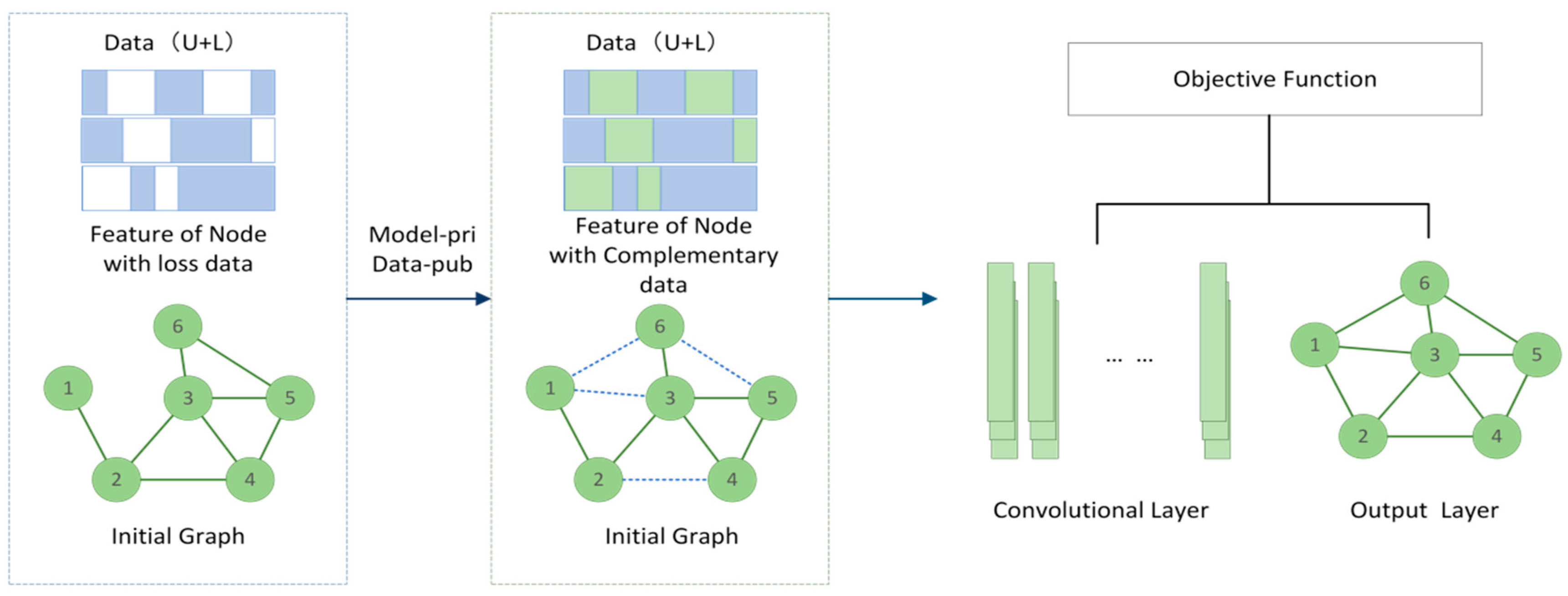
Figure 1.
A semi-supervised learning framework based on the GCN; the framework is described based on the three modules. It should be noted that the numbers in the node of the initial Graph and output layer are the given variable order in the sub-client.
Figure 1.
A semi-supervised learning framework based on the GCN; the framework is described based on the three modules. It should be noted that the numbers in the node of the initial Graph and output layer are the given variable order in the sub-client.

Figure 2.
The framework of the proposed method.

Figure 3.
(a) Impact of different epochs on annotation performance; (b) Impact of different epochs on annotation performance.
Figure 3.
(a) Impact of different epochs on annotation performance; (b) Impact of different epochs on annotation performance.


Table 1.
Set the loss under 90% missing data.
| Traffic Types | 1 | 2 | 3 | 4 | 5 | 6 | 7 |
|---|---|---|---|---|---|---|---|
| Car | 24.525 | 23.283 | 35.172 | 83.926 | 32.505 | 20.346 | 219.758 |
| Human | 0.184 | 1.45 | 40.799 | 2.858 | 2.478 | 0.438 | 48.208 |
| Bike | 1.724 | 54.245 | 27.948 | 64.191 | 18.209 | 124.879 | 291.197 |
| total | 5.391 | 17.432 | 36.847 | 32.565 | 11.944 | 31.797 | 135.975 |
| test | 20.931 | 32.202 | 33.667 | 57.806 | 64.350 | 47.454 | 256.41 |
Table 2.
Through data prediction and imputation, severely missing data were filled in and brought in for training again.
Table 2.
Through data prediction and imputation, severely missing data were filled in and brought in for training again.
| Traffic Types | 1 | 2 | 3 | 4 | 5 | 6 | 7 |
|---|---|---|---|---|---|---|---|
| Car | 1.127 | 4.467 | 6.792 | 8.211 | 9.692 | 14.421 | 44.71 |
| Human | 0.216 | 1.092 | 1.551 | 1.887 | 2.876 | 3.105 | 10.726 |
| Bike | 1.06 | 5.055 | 6.309 | 6.882 | 7.367 | 12.621 | 39.293 |
| total | 0.584 | 2.639 | 3.646 | 4.25 | 5.227 | 7.462 | 23.807 |
| test | 0.924 | 3.679 | 5.373 | 7.129 | 8.07 | 10.94 | 36.115 |
Table 3.
The accuracy of prediction after graph information interaction between subsidiary models.
| Traffic Types | 1 | 2 | 3 | 4 | 5 | 6 | 7 |
|---|---|---|---|---|---|---|---|
| Car | 0.409 | 0.742 | 1.108 | 1.494 | 1.856 | 2.26 | 7.869 |
| Human | 0.144 | 0.283 | 0.441 | 0.62 | 0.805 | 1.008 | 3.302 |
| Bike | 0.422 | 0.856 | 1.255 | 1.697 | 2.069 | 2.52 | 8.82 |
| total | 0.258 | 0.501 | 0.754 | 1.032 | 1.293 | 1.591 | 5.429 |
| test | 0.256 | 0.485 | 0.731 | 1.007 | 1.273 | 1.57 | 5.322 |
Table 4.
Model performances of different methods for trajectory prediction.
| Methods | V-LSTM | C-VGMM+VIM | GAIL-GRU | MMSI | DTSI | S-PLUS | Proposed Method |
|---|---|---|---|---|---|---|---|
| Accuracy (%) | 46.3 | 47.2 | 47.5 | 67.8 | 60.0 | 68.6 | 96.3 |
Table 5.
Compared model performances of the proposed method and three methods (MMSI, DTSI and S-PLUS) with different proportions of missing data.
Table 5.
Compared model performances of the proposed method and three methods (MMSI, DTSI and S-PLUS) with different proportions of missing data.
| Missing Data Proportion | MMSI | DTSI | S-PLUS | Proposed Method |
|---|---|---|---|---|
| 0 | 0.994 | 0.994 | 0.994 | 0.994 |
| 5 | 0.989 | 0.992 | 0.991 | 0.991 |
| 10 | 0.966 | 0.971 | 0.977 | 0.986 |
| 20 | 0.855 | 0.866 | 0.861 | 0.973 |
| 30 | 0.840 | 0.854 | 0.844 | 0.972 |
| 40 | 0.724 | 0.748 | 0.739 | 0.970 |
| 50 | 0.713 | 0.741 | 0.733 | 0.965 |
| 70 | 0.701 | 0.715 | 0.708 | 0.966 |
| 90 | 0.678 | 0.600 | 0.686 | 0.963 |
Disclaimer/Publisher’s Note: The statements, opinions and data contained in all publications are solely those of the individual author(s) and contributor(s) and not of MDPI and/or the editor(s). MDPI and/or the editor(s) disclaim responsibility for any injury to people or property resulting from any ideas, methods, instructions or products referred to in the content. |
© 2023 by the authors. Licensee MDPI, Basel, Switzerland. This article is an open access article distributed under the terms and conditions of the Creative Commons Attribution (CC BY) license (https://creativecommons.org/licenses/by/4.0/).
Share and Cite
MDPI and ACS Style
Yu, C.; Zhou, Y.; Cui, X. A Client-Cloud-Chain Data Annotation System of Internet of Things for Semi-Supervised Missing Data. Mathematics 2023, 11, 4543. https://0-doi-org.brum.beds.ac.uk/10.3390/math11214543
AMA Style
Yu C, Zhou Y, Cui X. A Client-Cloud-Chain Data Annotation System of Internet of Things for Semi-Supervised Missing Data. Mathematics. 2023; 11(21):4543. https://0-doi-org.brum.beds.ac.uk/10.3390/math11214543
Chicago/Turabian StyleYu, Chao, Yang Zhou, and Xiaolong Cui. 2023. "A Client-Cloud-Chain Data Annotation System of Internet of Things for Semi-Supervised Missing Data" Mathematics 11, no. 21: 4543. https://0-doi-org.brum.beds.ac.uk/10.3390/math11214543
Note that from the first issue of 2016, this journal uses article numbers instead of page numbers. See further details here.