Artistic Style Recognition: Combining Deep and Shallow Neural Networks for Painting Classification

Abstract

This study’s main goal is to create a useful software application for finding and classifying fine art photos in museums and art galleries. There is an increasing need for tools to swiftly analyze and arrange art collections based on their artistic styles as a result of the digitization of art collections. To increase the accuracy of the style categorization, the suggested technique involves two parts. The input image is split into five sub-patches in the first stage. A DCNN that has been particularly trained for this task is then used to classify each patch individually. A decision-making module using a shallow neural network is part of the second phase. Probability vectors acquired from the first-phase classifier are used to train this network. The results from each of the five patches are combined in this phase to deduce the final style classification for the input image. One key advantage of this approach is employing probability vectors rather than images, and the second phase is trained separately from the first. This helps compensate for any potential errors made during the first phase, improving accuracy in the final classification. To evaluate the proposed method, six various already-trained CNN models, namely AlexNet, VGG-16, VGG-19, GoogLeNet, ResNet-50, and InceptionV3, were employed as the first-phase classifiers. The second-phase classifier was implemented as a shallow neural network. By using four representative art datasets, experimental trials were conducted using the Australian Native Art dataset, the WikiArt dataset, ILSVRC, and Pandora 18k. The findings showed that the recommended strategy greatly surpassed existing methods in terms of style categorization accuracy and precision. Overall, the study assists in creating efficient software systems for analyzing and categorizing fine art images, making them more accessible to the general public through digital platforms. Using pre-trained models, we were able to attain an accuracy of 90.7. Our model performed better with a higher accuracy of 96.5 as a result of fine-tuning and transfer learning.

1. Introduction

The technique for semantic classification of images representing fine art paintings is addressed in this research using a multi-phased machine learning strategy. The proposed method demonstrates how a machine can effectively perceive a creative style. This research tends to review the semantic gap issue, possibly the most critical challenge in picture recovery and identification by machine. In general, image classification can be thought of as labeling an image to be placed in a particular category [1]. Images can be categorized according to “what they depict”, which varies depending on the kind of labels used. This is known as object recognition (for example, acknowledgment of scenes versus representations, dogs versus cats, kinds of written characters, etc.). The question “what is the meaning” of the image is the basis for the second kind of labeling, called semantic classification (for example, happy versus sad images, safe versus dangerous road scenes, and visually appealing scenes versus scenes that are not). Semantic classification, which is subjective and person-dependent, is still largely unknown, even though traditional machine learning methods can efficiently solve the object recognition task [2].

In both art history and computer science, categorizing fine art styles has long been a difficult task. There is a problem with this work that experts frequently refer to as the “semantic gap”. This phrase captures the stark contrast between the intricate and varied character of creative forms and the constraints of conventional approaches to art analysis and classification. The semantic chasm highlights how difficult it is to precisely define and categorize artistic expression, which is elusive and frequently subjective. Through the use of machine-based art classification, this study aims to close the semantic gap. We seek to fundamentally alter how we view and comprehend the many fine art genres through the use of cutting-edge technology and computational techniques. This project not only resolves the age-old problem of classifying various art forms but also opens up several revolutionary opportunities.

Highly qualified and skilled art professionals who have spent years of research and education on the particulars and tiny details of delicate art objects possess the skill to identify an artistic style in the paintings. These skills have a very exclusive character for many years because they need to be learned over a long period through exposure to the visual world. The increasing accessibility of online collections and digital sources has made fine art more readily available to the general public. This has created a demand for making art knowledge accessible to a broader audience. One approach to addressing this demand is to transfer the skills of human professionals to machines. Machines can be made capable of tagging and identifying the artistic genre of unknown images if they are trained with large datasets of fine art labeled by human professionals [3]. This enables the automatic retrieval of images, classifying art genres, and labeling unlabeled images in art museums. Additionally, machine-based art knowledge can be applied to finding lost art or creating robots with a sense of aesthetics and appreciation for art similar to humans. When classifying paintings, the most common semantic criterion is style. Style is defined in the visual arts as a group of distinguishing features that can be linked to a specific artistic style, thought, or era [4]. However, even for experts, categorizing a painting’s distinct stylistic category can be challenging. A portion of the difficulties incorporates the doubtful interpretability of unique and stylish components, nuances that separate different artistic categories, smooth changes of periods of art, and creative qualities that have attributes of numerous styles or have a place with no style [5,6].

Automatic art classification has gathered increasing interest over the past ten years, and deep learning methods have played a prominent role in addressing this problem. These methods often employ transfer learning or fine-tuning techniques using various pre-trained CNNs. Transfer learning is the process of customizing a pre-trained CNN model that has been trained on a sizable dataset (like ImageNet) for a particular job, such as painting classification. By leveraging the knowledge learned from the pre-training, CNN can effectively extract meaningful features from paintings and classify them into different categories [7]. This approach has shown promising results compared to traditional methods that focused on manually determining the best set of characters to be drawn from art objects for classification. Deep learning models have demonstrated the ability to automatically learn hierarchical representations of data, allowing for more effective feature extraction and classification. Furthermore, some non-network classifiers, such as SVM or random forests, can be trained using features extracted by finely tuned CNNs. By combining the power of deep learning for feature extraction with traditional classification algorithms, researchers have explored different methods to improve the accuracy of art classification [8]. Transfer learning is a technique that allows the adaptation or reuse of an already trained network model. This was developed using an extensive dataset for a specific task to perform a similar task with a smaller dataset.

In painting style classification, transfer learning enables the modification of complex network models that have been pre-trained on large datasets of natural images to classify painting styles. The advantage of transfer learning is that it significantly reduces the training time required and utilizes smaller datasets compared to the original pre-training task. By leveraging the knowledge and representations learned from the large dataset, the network model can be fine-tuned to perform style classification on paintings. Deep learning techniques have shown positive results in painting style classification, although they were not as successful as in image object recognition tasks. Most studies utilize standard CNN architectures, for which an image of fixed size is required, which can have a lower resolution than the images present in datasets [9]. Consequently, the analyzed paintings need to be resized to fit the expected input dimensions, which can result in geometric deformation and content distortion, and relevant details can be lost. This downsizing process can damage the accuracy of the method used for classification, as it may lead to a loss of texture and compositional details, such as brushstroke position, orientation, length, and width, as well as variations in light, color, and shape. To address the challenges posed by fixed input image sizes in fine art style classification, a sub-region technique is used.

With this method, the original image is divided into patches with sizes that correspond to the CNN model’s default image input size. This approach offers several advantages. It allows for a more detailed examination of different regions within an artwork, capturing fine-grained information and preserving important artistic details. This approach considers that different painting regions may exhibit distinct style characteristics [10]. Based on this sub-region approach, a two-phase painting classification strategy is proposed in this research. The first stage of the suggested method involves segmenting the image into patches and using a deep neural network (NN) to train and identify each patch independently. This allows for a localized analysis of style within the artwork. In the second phase, a shallow neural network is employed. It is trained on the probability vectors provided by the first-phase classifier. This second-phase classifier combines the results from each patch to generate the final style label for the entire artwork. The suggested technique is assessed and compared with existing strategies using three fine art databases [11]. To understand the impact of different levels of complexity, six well-known CNN models are tested as the first-phase classifiers. The results of the proposed method are compared with the performance of other recent methods in the field. By adopting the sub-region approach and utilizing a two-phase classification strategy, this research aims to improve the accuracy and effectiveness of fine art style classification. The evaluation and comparison with existing methods provide insights into the performance and capabilities of different CNN models for this task.

1.1. Research Questions

This study’s principal research questions include the following:

• Can visual cues be used to accurately define fine art forms using machine learning algorithms?
• How might the robustness and accuracy of style categorization be increased by the use of deep learning techniques?
• What effects will automated art classification have on the market for fine art, cultural preservation, and art history?

We aim to shed light on the potential of machine-based art classification to offer new perspectives on art history, aid cultural preservation, and enlighten the art market, in addition to improving the accuracy of categorization. By highlighting the symbiotic relationship between technology and the humanities and how it might improve our comprehension and appreciation of great art, this research adds to the continuing conversation in the domains of computer science and art history. The purpose of this research is to create a machine-learning model that can correctly categorize paintings into predetermined categories following their artistic qualities. Style, genre, age, and perhaps even the creator’s identity are examples of qualities.

1.2. Contributions

The following are a hybrid model’s significant contributions:

• We divided the proposed approach into two independently trained classification phases.
• In the initial phase, a deep convolutional neural network is employed, which is trained directly on the image data. This phase aims to learn and extract relevant features from the images indicative of different artistic styles. The deep CNN is capable of capturing complex visual patterns and representations.
• A shallow neural network (NN), which is trained using the class probability vectors produced by the first-phase classifier, is used in the classification process in the second phase. Instead of working directly with the image data, this phase operates on the probabilities assigned to each artistic style by the first-phase classifier.
• To ensure a comprehensive analysis, six different CNN models with varying architectural complexities were utilized.
• According to the research findings, we combined local patch-based analysis with a comprehensive analysis of the complete image to produce the greatest results for stylistic art analysis.

The remaining sections of the paper are as follows:

• Section 2 provides a comprehensive overview of previous research on style painting classification. It covers the various techniques and methods in this field, highlighting their strengths and limitations.
• Section 3 describes the proposed method for style painting classification.
• Section 4 focuses on the experiments conducted to evaluate the proposed method.
• Section 5 finally concludes with a summary of the main findings and contributions.

2. Related Work

This section offers a thorough discussion of the many methods for classifying fine art styles, including both conventional and deep learning techniques. We will group this study by approach and add critical analysis and method comparisons to make it easier to read and understand. The problem of categorizing fine art has been approached through various methods, broadly categorized into traditional and deep learning (DL) strategies. Details of these two groups are discussed below:

2.1. Traditional Approaches

The foundation of this discipline has long been established by conventional methods of art classification. These techniques frequently rely on human feature extraction and professional curation. In classical approaches [12], the process of style classification begins with extracting a set of low-level image descriptors from the input artwork. These descriptors capture specific visual features, such as color, texture, shape, or local vital points. Once the descriptors are extracted, they are input to standard classification algorithms. These algorithms can include decision trees [13], SVM [14], kNN [15], or other statistical classifiers [16]. The classification algorithm compares the extracted features with a pre-defined set of style categories and assigns the artwork to the most appropriate class based on the similarity of features. These traditional methods rely on carefully handcrafted features and use well-established classification algorithms to categorize fine art based on style. However, their performance may vary depending on the choice of descriptors and the effectiveness of the classification algorithm.

2.2. Deep Learning Strategies

Deep learning has significantly improved art classification, thanks to the strength of neural networks and massive data. In preceding years, deep learning strategies, particularly convolutional neural networks (CNNs) [17], have gained popularity in fine art style classification. With deep neural networks, these DL techniques can automatically learn hierarchical representations from unprocessed image data. In DL-based approaches, the CNN models are typically trained on significant datasets, such as ImageNet, using millions of natural images. The pre-trained models [18] capture general visual features and can be fine-tuned or adapted for fine art style classification using transfer learning techniques. The pre-trained CNN models learn to recognize abstract visual patterns and textures, enabling them to capture complex style characteristics. By utilizing deep learning techniques, these models can automatically learn relevant features directly from the artwork images, eliminating the need for handcrafted descriptors. This allows for more effective and data-driven representation learning, potentially improving the accuracy of style classification. Accuracy, scalability, interoperability, and data requirements are all evaluated, and it becomes obvious that while deep learning approaches have revolutionized the classification of art styles due to their higher accuracy and scalability, they also pose problems for interpretability and data requirements. Even though they have limitations, traditional approaches provide insightful interpretations and can be helpful when there is a dearth of labeled data. The future of art classification may lie in combining the two methods, successfully utilizing their individual strengths to close the semantic gap.

Previous research tried the plausibility of painting genre classification on tiny datasets of images and utilizing a couple of style classifications. A dataset of 513 images was used to classify three styles, as shown in [19]. A method known as “weighted nearest neighbor (WNN)” was used as a classifier, and several transforms, including Fourier, Chebyshev, and wavelet, were used to extract the features. Different instances of significant works in light of the extraction of low-level features incorporate techniques proposed in [20,21]. In the previous study, a training dataset comprising 490 paintings was utilized to draw out features and classify seven distinct art genres. The classification process employed methods such as the opponent scale-invariant feature transform (O-SIFT) and the color scale-invariant feature transform (CSIFT) algorithms. Similarly, the latter study employed a dataset called Painting-91, consisting of 4266 images across 13 styles. Various feature-extraction techniques were implemented, including color local binary patterns, local binary patterns (LBPs), generalized image search tree (GIST), histogram of oriented gradient (HOG) parameters, pyramid of histograms of orientation gradients (PHOGs), and scale-invariant feature transform (SIFT). To classify the extracted features in both studies, the SVM algorithm was employed. Multi-class classification results with low-level features were lacking [20,21]. In [22], various combinations of features and classifiers were investigated. In [23], the focus was on investigating the order of three art styles based on subjective variety descriptors and similarity.

This investigation utilized classifiers such as support vector machines (SVMs) and k-nearest neighbors (k-NNs). However, no significant advancements were achieved in any of these instances. Furthermore, in another study [24], the classification of 6777 paintings into eight style groups was explored by investigating unsupervised feature extraction techniques. Unfortunately, no noteworthy progress was made in this endeavor. However, the field experienced a breakthrough when researchers started incorporating deep learning (DL) methods. By leveraging convolutional neural networks (CNNs) pre-trained on vast image datasets, significant advancements were finally achieved in image classification tasks. Recent research in the field of style classification has been dominated by pre-trained and fine-tuned CNN models, which possess the capability to learn features and infer style labels effectively. Transfer learning, which involves fine-tuning a pre-trained network using a small dataset, has played a crucial role in achieving these advancements. In this process, a pre-trained CNN is adapted to serve as a feature extractor within various deep-learning methods [25,26,27,28,29,30,31]. Notably, introducing pre-trained CNN models brought about a shift in determining knowledge-based features. Instead, the features were represented by the parameters of the network itself.

To classify these network parameters, linear classifiers like support vector machines (SVMs) were commonly utilized. A significant and comprehensive investigation of artistic work grouping was reported in [25]. This study covered an extensive range of artistic works, demonstrating the substantial scope of the research conducted. Studies in this subject have consistently yielded accurate classification results utilizing features generated by a pre-trained CNN model on a sizable dataset of paintings representing 25 styles. The SVM was employed as the classifier of choice. Remarkably, these studies demonstrated that DL-based style classification models surpassed classical models based on knowledge-based features. For instance, in [31], the efficiency of feature extraction using pre-trained CNN models was compared to the efficiency achieved using a comprehensive collection of hand-designed visual descriptors. The results revealed that the CNN-based feature extraction method outperformed other approaches significantly. Furthermore, transfer learning was applied to enhance style classification by leveraging the same CNN model for feature learning and label inference. This technique improved the accuracy and performance of the style classification models. The work by [32] stands as one of the pioneering systematic studies employing the method of utilizing pre-trained CNN models for style classification. Their study involved many paintings, encompassing more than 27 stylistic categories.

The AlexNet, a pre-trained CNN originally designed for object classification, was used in this research. Notably, it was demonstrated that training the CNN model “from scratch” yielded superior results compared to typical non-network classifiers trained using CNN-derived features. Subsequent studies [33,34] conducted similarly have consistently confirmed these findings. The use of pre-trained CNN models for style classification has proven highly effective, surpassing the performance of traditional classifiers trained on CNN-derived features. In [35], the suggestion was made that object classification data could potentially lead to better results compared to using transfer learning with an initial image recognition or sentiment analysis training for the CNN model. The authors proposed that using specific data related to object classification tasks could improve the performance of the CNN model. On the other hand, ref. [36] focused on studying style order results from calibrating three separate CNN models. Principal component analysis (PCA) is used by researchers to learn and analyze CNN representations of artistic styles. The findings of this study indicated a strong correlation between the chronological order of paintings and the features extracted by the CNN models.

In [37], the study focused on painting recognition using image patches. Specifically, binary identification of Van Goh’s painting was performed. The approach involved utilizing an SVM model trained with features extracted from a CNN model. A smaller dataset consisting of 332 paintings was used to train the CNN. Each analyzed image was divided into patches, and each patch was assigned a unique classification. The highest-scoring categorization patch was used to make the final decision about the painting. Moving on to [38], this study investigated image analysis using datasets containing images of varying sizes. The researchers employed autonomous CNNs trained on various image scales and calculated the average score across these models to create images of artworks based on artist recognition. This approach aimed to handle images of different sizes effectively. In a similar study, [39] proposed a three-layer multi-scale pyramid framework for artist recognition. The first layer of the CNN examined fixed-sized input images from input photos expanded by two and four times. The second layer read four patches, while the third layer considered sixteen patches. The category with the highest average class entropy was the basis for the choice.

In [40], an intriguing patch-based approach was proposed for classifying paintings based on their style. The study utilized a dataset of 2337 images with 13 different style groups to train a complex three-branch CNN architecture. The CNN received three random patches as inputs. Three patches were created: two from the original image and one from a scaled-down version of the same image. This approach aimed to capture style-related information from different parts of the artwork. In [41], a different approach was suggested for classifying artistic styles across a large image dataset. The study employed a boosted ensemble of SVMs and utilized color histograms and image topographic descriptors as features. The classification results from analyzing the entire painting, and a few random sub-regions were combined using majority voting to decide on the painting’s style. 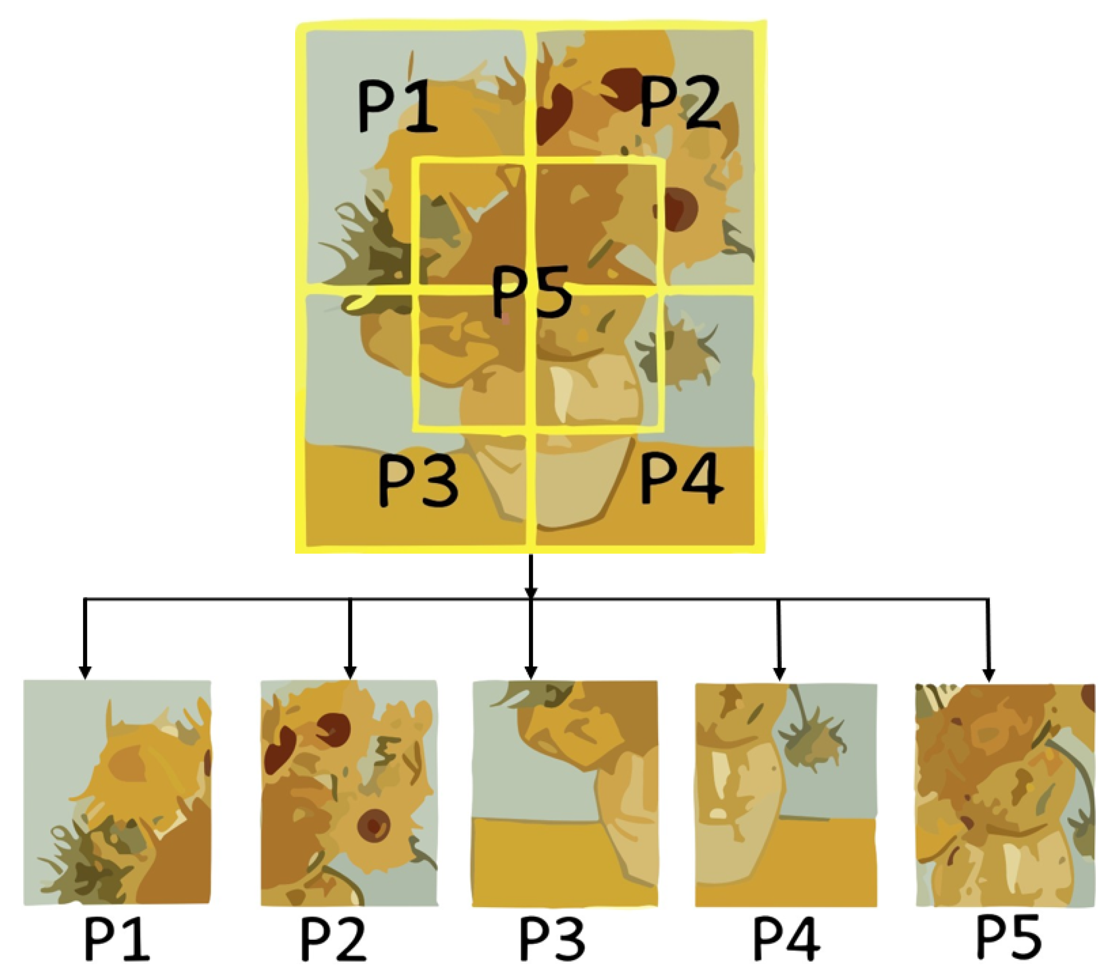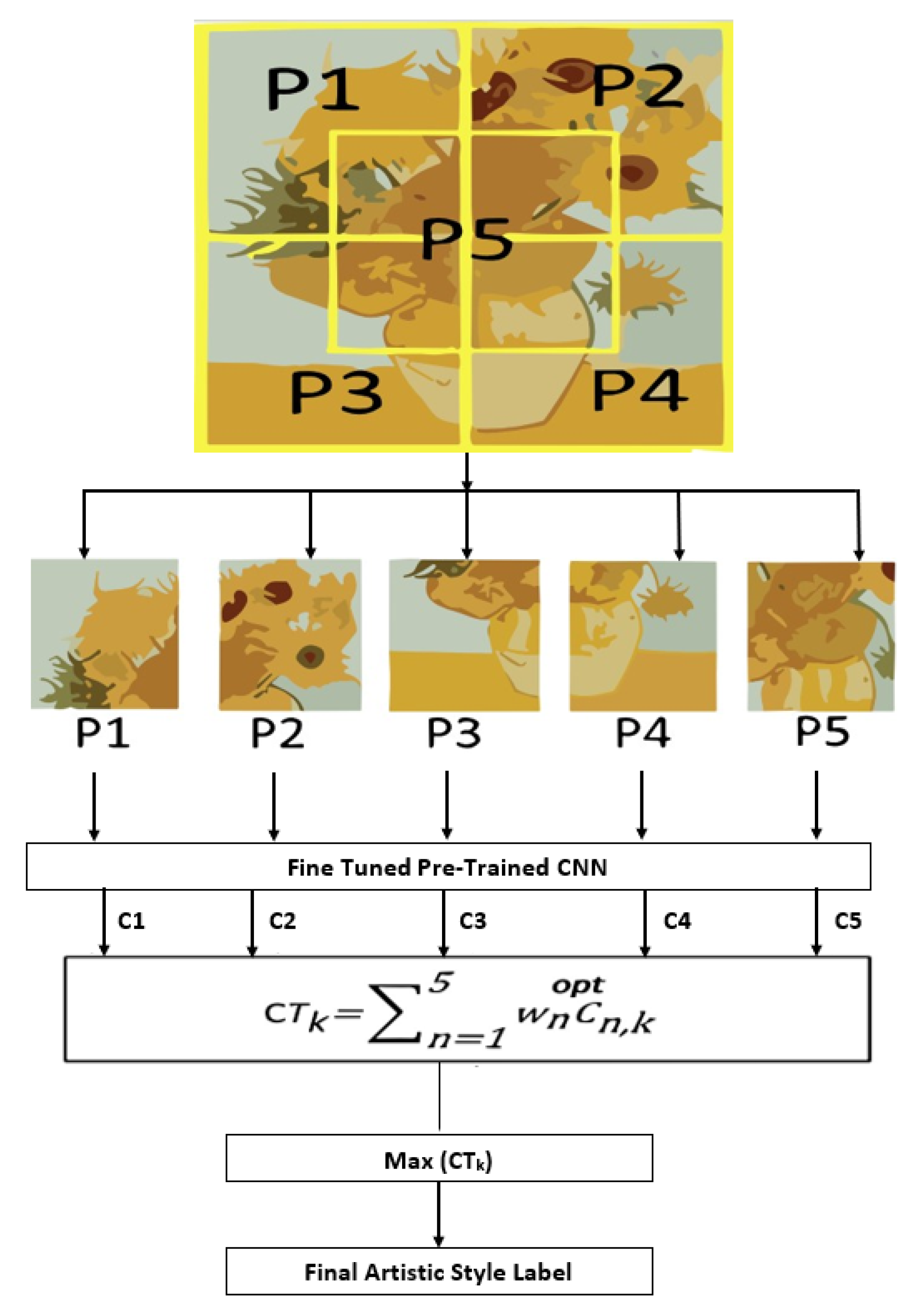In [42], it was demonstrated that incorporating a sum of outcomes for individual patches can greatly enhance classification results. The study utilized a CNN to classify each patch independently, and then an average of the classification results was calculated to choose the ultimate style label. The values were determined using mathematical optimizations to enhance the overall accuracy of style ordering. This optimized approach significantly improved the accuracy of style classification. Building on this, in our proposed method, we introduce a two-phase characterization calculation that further enhances the results of patch-based style characterization. This two-phase process aims to provide additional improvements in accurately classifying artistic styles based on fixed image regions.

3. Methodology

The proposed two-phase classification system for fine-art style classification draws inspiration from patch analysis and the multi-stage classification technique described in [43]. It involves dividing artwork into patches, classifying each patch using a deep neural network in the first phase, generating probability vectors for each style class, and performing a second-phase classification using a shallow NN or another classifier to produce the final style label for the entire artwork. This approach aims to improve the accuracy and effectiveness of style classification by considering localized style characteristics and overall style patterns in the artwork. An artificial neural network with a minimal number of layers between the input and output layers is known as a shallow neural network (shallow NN). An input layer, one or more hidden layers, and an output layer are the typical components, as shown in Figure 1. For tasks like classification, regression, and pattern recognition, shallow NNs are frequently utilized [44]. Shallow neural networks (NNs) are appropriate for many machine learning tasks, but they might not be as effective for challenging issues such as deeper structures, like deep neural networks (DNNs) or convolutional neural networks (CNNs). They are a useful option for some applications since they require less calculation and are simpler to read.

Shallow NNs have one or more buried layers with many neurons in each layer. Using weights and biases, these neurons modify the input data in linear and nonlinear ways. The architecture of the network (such as how many hidden layers to utilize) and the number of neurons in each hidden layer are normally decided through experimentation and domain expertise. Shallow NNs can act as foundational models for increasingly difficult problems. We utilized a shallow neural network because it is straightforward and requires less computation. Shallow NNs demand less processing power for both inference and training. A family of neural networks called deep convolutional neural networks (CNNs) is intended for processing and categorizing visual data, notably images. These networks are increasingly being used for computer vision applications like picture segmentation, object detection, and classification. An outline of the architecture and parts generally present in a deep CNN can be found here: input layer, convolutional layers, activation function, output layer, dropout layer, batch normalization, and optimizer. Different architectures for deep CNNs are possible, each with a unique number of layers, filter sizes, and layer configurations. Popular CNN architectures with distinct design philosophies include VGG, ResNet, and Inception. These networks are frequently utilized as the foundation for transfer learning in a variety of computer vision applications because they have already been pre-trained on big-picture datasets. The applicability of deep convolutional neural networks (DCNNs) and shallow neural networks (SNNs) relies on the particular problem and dataset. Both have special benefits and drawbacks.

3.1. Advantages and Disadvantages of DCNNs and Shallow NNs

DCNN Advantages:

• DCNNs are very adept at learning hierarchical data representations in computer vision tasks. They automatically extract significant features at various abstraction levels.
• On benchmark datasets, DCNNs have demonstrated state-of-the-art performance in image-related tasks like image classification, object detection, and segmentation. They are effective at managing complicated and big databases.
• Smaller datasets can be used to fine-tune pre-trained DCNNs (like VGG and ResNet) on certain tasks, yielding noticeable performance increases and needing less data than training from scratch.
• DCNNs are suited for a variety of computer vision applications since they can handle huge and high-resolution images.

DCNN Disadvantages:

• It can be computationally expensive to train and use DCNNs, particularly for deep architectures. A lot of processing power and specialized gear, like GPUs, may be needed for this.
• DCNNs are less useful for smaller datasets since they frequently need a lot of labeled data to train effectively.
• Deep neural networks, particularly DCNNs, are frequently regarded as “black-box” models, making it difficult to understand how they produce predictions.

Shallow NN Advantages:

• Shallow neural networks are easier to understand since the connections between input and output are relatively simple. They are therefore valuable in applications where it is critical to comprehend the model’s decision-making process.
• SNNs require less processing power than deep networks. They are relatively simple to train and utilize using common hardware.
• Shallow networks are advantageous when data is scarce since they may perform effectively with fewer datasets.
• SNNs can be used to solve a variety of issues, including regression, classification, and time-series forecasting, and are not just applicable to picture data.

Shallow NN Disadvantages:

• Shallow networks might have trouble detecting intricate hierarchical patterns in data. They use manual feature engineering, which can take a lot of time.
• SNNs might not perform as well as DCNNs, which can automatically learn rich representations, in jobs involving high-dimensional data or complex patterns.
• Overfitting can occur in shallow networks, especially when the dataset is limited and the feature space is high dimensional.

In summary, DCNNs excel in autonomously learning hierarchical features, making them particularly well-suited for jobs involving complicated visual data and big datasets. They do, however, have computational and data needs. SNNs are advantageous for short datasets or where comprehending the model’s decisions is crucial because they are more interpretable and computationally economical. The particular specifications and characteristics of the current challenge should serve as a guide for deciding between DCNNs and SNNs.

3.2. Breakdown of Different Phases

The classification of styles in the proposed method involves two phases. Here is a breakdown of each phase and its components:

• Image Division: The input image is divided into five patches or sections (P1–P5). This division allows for a localized style analysis within different image regions.
• Deep CNN Classification: It uses a deep convolutional neural network CNN model to categorize each patch’s artistic approach. The CNN model can learn and extract style cues from the input patches since it has been trained on a sizable dataset of labeled photos.
• Probability Vector Combination: The classification results from the first phase, in the form of probability vectors (C1–C5), are collected and combined into a single input vector.
• Shallow NN Classification: In the second phase, a shallow neural network or another classifier is employed to classify the combined probability vector and produce the ultimate style label for the input image. The probability vectors generated from the initial phase classification are used to train this classifier.
• Images are used to train the deep CNN classifier in the first step from a labeled dataset, allowing it to learn to classify individual patches based on their style.
• The second phase shallow neural network classifier is trained on the class-probability vectors generated by the first phase classification. It learns to assess the classification abilities of the first-phase classifiers and make the final style decision based on the combined information.

By utilizing both phases, the proposed method incorporates the expertise of multiple “assessors” (the first phase classifiers), which evaluate different parts of the image. In the second phase, the classifier learns to assess the classification abilities of these assessors and make the final decision based on their input. In the following sections, this research provides a more detailed analysis and explanation of the individual components of the proposed method.

3.3. Phase 1—Patch Extraction

In the image, five patches have been identified. Before dividing the image into these patches, it is necessary to scale up the image by a suitable factor to ensure that the size of the patches aligns with the requirements of a specific CNN model. The first four patches correspond to different image sections: P1 represents the upper right section, P2 represents the upper left section, P3 represents the lower right section, and P4 represents the lower left section. The fifth patch, P5, is distinct as it encompasses the focal point of the artwork as shown in Figure 2. P5 covers 25% of each of the other four patches, indicating that it overlaps with all of them. To meet the input requirements of the CNN model, the image is scaled up before being divided into patches. The scaling factor will depend on the desired patch size specified by the CNN model’s input requirements.

3.4. Phase 2— Deep CNN Classifier

During the initial synchronization PHASE, Sync 1, the five patches (P1–P5) are individually inputted into a specific CNN model known as Classifier 1. The objective of this PHASE is to obtain intermediate style classification results for each patch, denoted as C1, C2, C3, C4, and C5. Bypassing each patch through Classifier 1, the model performs style classification on a localized level, focusing on the distinctive characteristics within each patch. The output of Classifier 1 provides information about the artistic style of each patch, capturing the style-related features specific to that particular region of the image. Sync 1 allows for the independent classification of each patch, enabling a more detailed analysis of the artwork’s style on a localized basis. The results obtained from Classifier 1 for each patch serve as the basis for the subsequent phases in the overall classification process.

Two options exist for training the CNN model: starting from scratch or using transfer learning with a pre-trained model. The choice depends on the available computational and data resources. Transfer learning is effective when resources are limited as it leverages the knowledge gained from pre-existing models. Training from scratch requires significant training time and data. During transfer learning, the last three layers of the pre-trained CNN model are adjusted to align with the desired style classification task. These layers comprise the classification output layer, the softmax layer, and the final fully linked layer. The size of the last fully connected layer depends on the number of distinct artistic styles considered in the classification. The softmax layer plays a crucial role in producing a vector representing the probabilities of each patch belonging to different potential artistic style classes. The softmax function normalizes the output values, providing a probability distribution over the style classes.

In the second synchronization PHASE, denoted as Sync 2, the output vectors $C_{i,j}$ (where i represents the input image index, j represents the patch number, and k represents the style index) contain the style probabilities $P_{i,j,k}$ with every patch j of the specified image I. These probabilities are computed for each style index k using Equation (1):

$$C_{ij}=p_{ijk}$$

(1)

for K = 1, …, L − (i) The classification output layer assigns each patch to a mutually exclusive stylistic category based on the highest probability value.

3.5. Phase 3—Assembling of Probability Vectors

In PHASE 2, the probability vectors $C_{i,j}$, which correspond to patches belonging to the same image I, are combined into a single vector called $I_i$. This concatenation operation is represented by Equation (2): Here, pi, j, k represent the probability of patch j in image i belonging to artistic style k. The concatenated vector Ii contains the possibilities for all N patches and L artistic styles. The second phase classifier, Classifier 2 uses the resulting vector of probabilities, Ii, as its input features. Classifier 2 is a shallow NN that utilizes Ii to make the final style classification decision for the input image. Combining the probability vectors from each patch into a single vector, the second phase classifier leverages the collective information of all patches to generate the ultimate style label for the examined image. This two-phase approach ensures that the second-phase classifier compensates for any potential errors or inconsistencies made by the first-phase classifiers operating on individual patches. Overall, the concatenated vector $I_i$ derived from the probability vectors of all patches is employed as input for Classifier 2, facilitating the determination of the final artistic style classification for the input image as shown in Figure 3.

3.6. Phase 4—Shallow NN Classifier

The second classifier is crucial in generating the final style classification label in the two-phase process as shown in Figure 4. It accomplishes this by utilizing the probability vector Ii, acquired from PHASE 3, as input features. Both phases of the process are trained concurrently. The first phase entails training a CNN model that produces style probabilities as its output scores. The second phase classifier, a standard classifier, employs these CNN training scores as input features during its training phase. The double classifier must be trained to use the style probabilities efficiently obtained from the first phase to classify styles accurately. After introducing both classifiers, the same two-phase procedure may determine the label for an unlabeled input image. The second stage classifier uses the probabilities produced by the first phase CNN as features.

4. Results and Discussion

4.1. Dataset

Machine learning largely depends upon the data. High-quality training must be applied to the charter; otherwise, even the best algorithm would not yield the desired results. Therefore, high-quality training data is the most fundamental aspect of machine learning, and training data shows the original data used in the model. In the present research, supervised learning was employed to guide the module with indicated trading data. When the data is labeled, the same dataset is segregated with fundamental identification features. These features are helpful for the module to learn and train. Hence, can we argue that the ability of the bottle to know the outcomes and execute high-quality predictions will mainly be affected by the extractor features from the datasets and the quality of labeling. The dataset is taken from Kaggle. To validate the efficiency of the suggested technique, three datasets comprising digital images of paintings were utilized. These datasets were obtained from publicly accessible art collections. Additionally, the authors of the technique created an additional dataset focused explicitly on Australian native art. By incorporating multiple datasets, the evaluation process encompassed various artistic styles and genres. Including the Australian Native Art dataset demonstrates the authors’ efforts to encompass diverse cultural artwork within the validation process. By applying the proposed technique to these datasets, the authors could assess its efficiency and determine its suitability for performing style classification tasks on computerized images of paintings.

4.1.1. Dataset 1

The initial dataset had 30,870 images, each representing a distinct artistic style. To ensure balanced representation, adjustments were made to the expressive classes. Consequently, each class was composed of 5145 pictures, accounting for approximately 16.67% of the total images. The expressionism, impressionism, post-impressionism, Australian Aboriginal art, realism, and romanticism aesthetic movements were chosen for the classification work.

These styles were carefully selected from the extensive WikiArt dataset [45] based on their availability of a substantial number of images, ensuring an adequate representation of Aboriginal-style images within the dataset as shown in Figure 5. This selection process aimed to create a balanced and comprehensive collection of artistic styles for accurate classification. Due to the nature of the WikiArt dataset, where the images were labeled by volunteers from the general public rather than art professionals, a manual verification process was implemented. This involved examining the labels for accuracy and eliminating non-fine art or low-quality paintings from the dataset.

4.1.2. Dataset 2

The main objective of Dataset 2 was to include a broader range of art styles as shown in Figure 6 compared to Dataset 1. Similarly to Dataset 1, the Australian Aboriginal paintings in Dataset 2 were primarily sourced from the WikiArt collection. The initial WikiArt collection contained over 85,000 paintings, categorized into 27 different styles. However, there was a notable disparity in the number of images representing each style, ranging from 12,000 to only 98 images per style [45].

To address this imbalance, 23 out of the 27 categories of style taken from the WikiArt database were selected, aiming for a more equitable representation. Additionally, three classes related to cubism were combined into a single class, resulting in a total of 21 WikiArt styles. In addition to the Australian native style, Dataset 2 comprised 26,400 images across 22 styles. Each style was allocated 1200 images, corresponding to 5% of the total number of images. This approach ensured a balanced representation of styles while also considering the computational resources required to analyze the images within the limitations of the present hardware. Figure 7 illustrates the distribution of styles in Dataset 2.

4.1.3. Dataset 3

Images of paintings from the Paintings Dataset for Categorising the Art Movement (Pandora 18k) were included in Dataset 3. The creative movements were categorized using these images. The dataset’s features could be classified using various methods, including a multiclass support vector machine (SVM), a Gaussian mixture model (GMM), or a shallow neural network. These techniques enable the classification and recognition of different art movements based on the features extracted from the images. Dataset 3 included images from the Pandora 18K dataset [46,47] in addition to the Australian original style. The dataset comprised a total of 19 styles and 19,320 images. Figure 8 visually represents the distribution of images among the different styles, showcasing a relatively balanced number of images for each style. One of the Pandora 18K dataset’s key advantages was its high label validity level; unlike the WikiArt collection, where the public generated labels, the labels in the Pandora 18K dataset were assigned strictly by art experts. This ensured greater accuracy and reliability in the labeling process, enhancing the quality and trustworthiness of the dataset.

4.2. Research Methodology

The overall flow of the project is presented in Figure 9, which shows the stages involved in the implementation of the research, from data collection to evaluation of the results.

4.3. Calculation Formulas for the Evaluation Matrices

• Precision: Precision is the ratio of correctly predicted positive classes to all correctly and incorrectly predicted positive classes made by the model.
• Recall: Recall is the proportion of positive observations projected to occur to all other positive observations.
• F1-Score: The F1-score is determined by averaging precision and recall over a weighted period.

4.4. Experimental Setup

The experimental set-up utilized for evaluation and testing is shown in

Table 1. Experimental Setup.

Parameters	Value
Libraries	Numpy, Panda, TensorFlow, and PyTorch
Datasets	Australian Native Art dataset, WikiArt dataset, ILSVRC, and Pandora 18k.
Australian Aboriginal art	30,870
WikiArt	85,000
Pandora 18K	19,320
ImageNet	1.2 million
Platform	Jupiter Notebook
Languages	Python
Single Node System, Configuration	RAM 8GB, Intel Core i7

. To evaluate the proposed approach, six popular CNN architectures, namely VGG-16, AlexNet, VGG-19, ResNet-50, Inceptionv3, and GoogLeNet, were employed. The ImageNet Large Scale Visual Recognition Challenge (ILSVRC) dataset served as a pre-training ground for these architectures, consisting of approximately 1.2 million labeled images covering 1000 classes. By leveraging the knowledge captured through pretraining on ImageNet, the models possess a broad understanding of visual patterns and objects. This transfer learning approach enables the proposed method described in Figure 10 to benefit from the expertise and capabilities of these well-established models, avoiding the need for training from scratch. Utilizing these pre-trained CNN architectures shown in Figure 11 allows for a comprehensive evaluation of the proposed approach using state-of-the-art models that have demonstrated effectiveness in various computer vision tasks.

The final three fully connected layers of each network were changed to accommodate the number of classes in the target dataset to modify these CNN models for artwork style recognition. These adjusted models were then fine-tuned to optimize their performance in recognizing artwork styles.

Table 2. CNN model Characteristics.

Model	No. of Layers	Architecture	Input Size	Size in MB	Parameters (Millions)
AlexNet	8	Linear	227 × 227	227	61
VGG-16	16	Linear	224 × 224	515	138
Vcg-19	19	Linear	224 × 224	535	144
GoogleNet	22	Inception Model	224 × 224	27	7
ResNet-50	50	Residual Blocks	224 × 224	94	25
Inception V3	48	Inception Model	299 × 299	88	23

provides an overview of the CNN models’ key characteristics. Among the evaluated CNN architectures, GoogleNet, ResNet-50, and Inceptionv3 stand out with their more intricate and deeper designs, incorporating non-linear components like inception modules or residual blocks. In contrast, VGG-16, AlexNet, and VGG-19 follow a sequential architecture. These variations in architectural complexity provide a diverse set of models to assess the proposed approach, offering insights into the performance and suitability of different CNN designs for the given task. To train and evaluate the CNN models, 80% of the dataset was utilized for training, while the remaining 20% was used for testing the system’s performance.

The classification accuracy was evaluated using a three-fold cross-validation scheme. The average accuracy across all folds was calculated and reported as the final result. To obtain the overall accuracy, the average of all testing patches or samples was computed, providing a comprehensive assessment of the model’s performance.

4.4.1. Case 1—Baseline

A single-phase classification approach was employed, and the input images for the CNN models were not divided into patches. Instead, each image was resized to fit the required dimensions of the respective CNN architecture. The precision of each CNN model was determined by averaging the results across all analyzed images. This approach considered the overall performance of the models based on the average accuracy obtained from the complete images.

4.4.2. Individual Patches for Case 2

A single-phase classification method was used in Situation 1, but the input photos were treated differently. In example 2, the photos were separated into five patches. Using the matching style label, each patch was then separately classified. The framework treated these patches as separate entities since it did not grasp their connections. Each original image had to go through up-sampling, which doubled its size from the CNN input, to meet the demands of the CNNs before being separated into the five patches. This methodology allowed for examining the individual style characteristics in different image regions without considering any contextual information or interactions between the patches during the classification process. In contrast to the prior method, the split of the photos into patches resulted in a five-fold increase in the size of the training dataset. By taking a weighted average of the classification outcomes acquired for each of the five patches, which were represented as probability vectors, the categorization of a painting’s style was established. This weighted averaging method considered the influence of each patch’s classification result when determining the overall style of the painting. Rather than using majority voting or simply averaging the probability values, this approach assigned appropriate weights to each patch’s classification outcome, considering their relative importance in the final decision. This weighted averaging technique aimed to provide a more nuanced and comprehensive assessment of the painting’s style by incorporating the contributions of individual patches in a more balanced manner. To optimize the classification accuracy of the entire system, a numerical optimization algorithm was employed. This algorithm determined the optimal weight values with the highest possible classification accuracy.

4.4.3. Case 3: Voting by a Majority

The method used to partition the input photos into five patches and separately classify each patch to obtain style labels was the same in this test case as it was in Case 2. However, determining the final style label for each original input image deviated from the previous approach. Instead of taking a weighted average of the classification results, a different process was employed. The final style label for each original input image was determined using a straightforward majority vote among the five patch classification results. The style category that received the highest number of votes was assigned as the label for the entire painting in situations where, in the event of a tie between two or more labels, the label with the highest probability value was selected as the winner. This approach allowed for a democratic decision-making process, where the most frequently predicted style among the patches was chosen as the overall style label for the painting. The label with the highest likelihood value was used to break ties and determine the final style assignment when multiple styles received equal votes. The accuracy of each CNN model was assessed by computing the average of all the analyzed photos. This approach provided a comprehensive assessment of the models’ performance by considering the overall accuracy based on the average results obtained from all tested images.

4.4.4. Case 4—Average Probability

The average probability for each class was calculated across the five patches of an image in this case, comparable to Case 3, instead of using the majority voting method. The final label for that particular image was given to the class with the highest average chance. The average of all observed images was determined to assess each CNN model’s accuracy.

4.4.5. Evaluation Metrics

In the context of classifying paintings, or any other classification task, precision, recall, and F1-score are crucial evaluation measures. They aid in evaluating how well a machine learning model or system performs when classifying paintings into various groups or categories. Precision in the classification of paintings indicates the percentage of artworks that were accurately categorized inside a given category. High precision means that the model is typically right when it asserts that an artwork belongs to a particular category. Recall provides information on the percentage of paintings in a given category that were successfully classified in the context of classifying artworks. High recall indicates that the model does an excellent job of capturing the majority of the paintings in a given category.

$$Accuracy=\frac{TP+TN}{TP+TN+FP+FN}$$

(2)

Equation (4) allows us to assess the precision of each CNN model based on the average results obtained from all observed images.

Recall:

$$Recall=\frac{TP}{(TP+FN)}$$

(3)

where TP is true positive, and FP is false negative [48].

Precision:

$$Precision=\frac{TP}{(TP+FP)}$$

(4)

where TP is true positive, and FP is false negative [48].

Red

F1-Score: It is a harmonious method of recall and precision. As it becomes closer to 1, it displays a better value, and 0 indicates the poorest value for the F1-score. The metrics derived from recall and precision by applying [48]:

$$F1=\frac{2X\left(PrecisionxRecall\right)}{(Precision+Recall)}$$

(5)

Landscapes, portraits, abstract art, etc., are just a few examples of the various categories or classes that can be used to classify paintings. These metrics can be generated for each category to evaluate the performance of the model for each class independently. To obtain a comprehensive evaluation of the model’s effectiveness across all categories, it is possible to additionally compute micro- or macro-averaged versions of these metrics. These evaluation metrics assist researchers in determining how well your model is doing at categorizing artworks into the necessary groups while balancing the trade-off between precision and recall according to the needs of the application in question.

4.4.6. Weighted Average, Case 5

A different strategy was used in the revised patch categorization technique, which was motivated by Scenarios 3 and 4. A weighted average of the classification results obtained for each of the five patches was utilized rather than the majority vote or average probability value. An algorithm for numerical optimization was used to determine the ideal weight values to increase the system’s overall classification accuracy.

4.4.7. Proposed Two-Phase Classification in Case 6 Using Only Patches

The two-phase approach proposed in Chapter III was implemented in this case. Following the methodology outlined in Equation (2), based on the initial phase categorization, the probability vectors of individual patches within an image were combined to form feature vectors. These feature vectors were subsequently utilized as input for the second phase classifier to determine the final label for the analyzed image. This multi-phase process allowed for a more comprehensive analysis by capturing the combined information from the individual patch classifications and leveraging it to make a more informed decision regarding the overall label of the image. To identify the optimal second-phase classifier, preliminary tests were carried out using the probability vectors produced by AlexNet. Various classifiers were used to evaluate their performance, including coarse K-NN, subspace discriminant, a shallow NN, and multiclass SVM. After analyzing the results, the shallow NN was selected as the most suitable second-phase classifier. This choice was primarily influenced by the excellent performance demonstrated by the shallow NN, its high adaptability during training, and its relative ease of implementation. The shallow NN showed promise in effectively leveraging the probability vectors from the first phase classification, making it a favorable choice for the subsequent classification task in the proposed two-phase approach. The critical parameters of the shallow NN applied to each dataset are presented in

Table 3. Characteristics of the shallow NN classifier.

Dataset	No. of Layers	No. of Nodes	Probability Vector Size	No. of Categories
Dataset 1	3	3600	30	6
Dataset 2	5	2850/570	110	22
Dataset 3	5	2375/475	95	19

. A five-fold cross-validation approach was adopted to train the shallow NN, dividing the data into training, validation, and testing sets. Specifically, 66% of the data were allocated for training the shallow NN, 14% for validation to fine-tune the model’s parameters, and the remaining 20% for testing its performance. This data division ensured that the shallow NN was adequately trained, validated, and stretched across the datasets, allowing for reliable evaluation and comparison of its performance in different scenarios. Adopting a cross-validation approach helped mitigate overfitting and provided a robust assessment of the shallow NN’s generalization capabilities.

4.4.8. Proposed Two-Phase Classification for Case 7 Using Both Patches and the Entire Image

This case involves a methodology similar to the one Situation 6 utilized. However, in addition to classifying patches, the first-phase classification process also involved organizing the whole resized image. The resized image was adjusted to match the input requirements of the CNN model. This expansion in the first-phase classification is applied considering the overall style characteristics of the entire image alongside the style attributes present in the individual patches. By incorporating the category of the resized image, a more comprehensive analysis of the style was achieved, combining local and global information. This method sought to enhance the robustness and accuracy of the classification process while capturing a comprehensive grasp of the style components present in the image. By merging the patch probabilities with the image probabilities for diverse artistic styles, the feature vectors transmitted to the second-phase shallow neural network became more extensive. This occurred because the combined possibilities from multiple patches were concatenated or stacked together, resulting in longer feature vectors. These extended feature vectors incorporated the information from the individual patches and the overall image classification. In essence, the entire image was considered an additional “sixth patch” within the framework. By incorporating the complete picture as a distinct component, the classification process benefited from the holistic information captured by the image-level classification. This approach aimed to enhance the performance and accuracy of the system by considering both the individual patch-level details and the overall image-level characteristics within the feature vectors utilized by the second-phase shallow NN.

4.5. Flow of the Design Specification Process

Figure 12 depicts the three-tier architecture that was used to perform this project, briefly summarizing the procedures used as well as the technologies and tools employed.

4.5.1. Testing of Pre-Trained Model

In this final round of testing, some sample images were input with the help of the CNN, and the actual classes were compared with the predicted classes. We have shown the best accuracy results with the code segments in the

Table 4. Accuracy of Proposed Model.

Model	Accuracy (%)
CNN models	90.7
Shallow NN	96.5

.

4.5.2. Fine-Tuning and Training

Figure 13 demonstrates the fine-tuning process, where a previously generated CNN model is adapted to a new dataset using a low learning rate during the transfer learning phase. Through fine-tuning and training, more accurate results can be achieved because the model is retrained and then applied for testing. Figure 14 also illustrates the entire procedure and working of fine-tuning and training. During this process, the previously generated CNN model is utilized, excluding the output layer, which is adjusted to accommodate the number of target dataset classes. For instance, if the original model had two types and the new model required three categories, the output layer is modified accordingly. By applying fine-tuning and training, the model can learn from the new dataset while leveraging the pre-trained layers’ knowledge. The low learning rate ensures the model makes more minor weight adjustments during training, leading to a more refined and accurate outcome. By following this approach, we can observe improved results in terms of classification accuracy.

4.5.3. Testing

The performance of the new model was evaluated using a testing technique in the last phase. This involved running sample images through the convolutional neural network (CNN) and comparing the predicted and actual class classifications. By dividing the number of accurate predictions by the total number of test datasets, the validity of the results was established. Table 4 demonstrates the code segment that yielded the highest accuracy result of the transfer learning CNN model. This code segment as shown in Table 4 contains the necessary steps to load the pre-trained model, fine-tune it on the new dataset, and evaluate its performance on the test dataset. By analyzing the accuracy of the transfer learning CNN model, we can gauge how effectively it performs in classifying the images in the test dataset.

The overall outcome of the system is elaborated in

Table 5. Dataset 1: average classification accuracy (%) for various classification CNN model and cases.

CNN Model	Case 1	Case 2	Case 3	Case 4	Case 5	Case 6	Case 7
AlexNet	51.50%	48.50%	52.02%	53%	54.40%	61.53%	62.46%
VGG-16	52.80%	51.40%	53.10%	54.50%	56.04%	61.84%	62.69%
Vcg-19	52.90%	51.60%	53.40%	54.30%	55.90%	62.10%	62.81%
GoogleNet	54.50%	52%	55.50%	56.10%	57.60%	63.78%	64.42%
ResNet-50	56.80%	53.40%	56.90%	57.4%	58.50%	65.70%	66.64%
Inception V3	57.20%	54.50%	57.80%	58.30%	59.40%	66.18%	67.16%

,

Table 6. Dataset 2: average classification accuracy (%) for various classification CNN models and cases.

CNN Model	Case 1	Case 2	Case 3	Case 4	Case 5	Case 6	Case 7
AlexNet	49.30%	44.80%	51.15%	52.10%	54.50%	59.37%	60.27%
VGG-16	51.15%	47.60%	53.14%	54.60%	56.70%	61.17%	62.11%
Vcg-19	51.85%	48.10%	52.65%	55.10%	57.10%	61.57%	62.49%
GoogleNet	53.95%	50%	54.78%	57.20%	58.90%	63.37%	64.27%
ResNet-50	56.55%	51.80%	57.43%	58.90%	60.90%	65.13%	66.02%
Inception V3	57.10%	52.10%	57.97%	59.70%	61.70%	65.83%	66.71%

and

Table 7. Dataset 3: average classification accuracy (%) for various classification CNN models and cases.

CNN Model	Case 1	Case 2	Case 3	Case 4	Case 5	Case 6	Case 7
AlexNet	62.20%	57.30%	62.62%	63.50%	64.80%	72.04%	73.11%
VGG-16	63%	58.20%	63.15%	64.20%	65.30%	72.64%	73.61%
Vcg-19	62.87%	58.40%	63.01%	63.97%	65.07%	72.41%	73.36%
GoogleNet	64.10%	60.10%	64.43%	65.10%	66%	73.44%	74.37%
ResNet-50	65.97%	63.90%	66.57%	67.77%	68.57%	75.23%	76.14%
Inception V3	67.60%	63.40%	67.98%	69.40%	70.20%	76.57%	77.53%

. The suggested two-phase classification strategy demonstrated superior performance compared to other approaches in both Case 6 and Case 7. This improvement was observed across all CNN models and datasets, highlighting the benefits of employing a second-phase classifier trained on class-likelihood vectors rather than the original images. The second phase classification effectively compensated for the errors made during the first phase classification. It is important to note that the results of the first phase training were unaffected by the second phase training since both phases were trained independently. This implies that while the second phase may not significantly contribute to the overall performance if the first phase performs well, it also does not negatively impact the results achieved by the first phase. However, when the first phase exhibits subpar performance, possibly due to inadequate feature selection or training, the second phase can provide essential improvements without requiring the first-phase classifier to undergo extensive training with larger datasets. Moreover, it was observed that the second phase’s nonlinear modeling, accomplished through a neural network, outperformed more straightforward linear decision-making methods such as majority voting, average probability, and weighted average. This superiority of the nonlinear neural network modeling was consistently observed across all CNN models and datasets investigated.

The quality of the training dataset played a crucial role in determining the classification results. Among all methods and CNN models, Dataset 3 yielded the best performance as shown in Figure 14. Although Datasets 2 and 3 exhibited similar performance, they were approximately 10% less accurate than Dataset 3. This gap can be attributable to Dataset 3’s greater quality, which was curated using qualified knowledge and qualified labeling. Datasets 1 and 2, on the other hand, rely on volunteer non-expert annotations.

Figure 14 provides further evidence supporting the conclusions mentioned above. It compares the percentage precision of the proposed technique (Case 6) and the reference method (Case 1) when applied to different CNN models and datasets. The difference between the proposed method and the baseline method is more pronounced with higher CNN model complication and better-quality training data. By examining the contrasting outcomes between Case 6 and Case 2, the significance of incorporating the second-phase classification becomes apparent. The influence of this addition can be directly observed when comparing the outcomes. For instance, employing the simplest CNN model, AlexNet, the accuracy in Case 6, which involves two-phase classification, surpasses that of Case 2, which utilizes single-phase classification, by a notable margin. Specifically, for Dataset 1, Case 6 achieves a 12% higher accuracy than Case 2, while for Dataset 2, the improvement is 14%, and for Dataset 3, it reaches an even higher 16% increase.

These findings serve to emphasize the considerable enhancement achieved by integrating the second phase of classification, leading to an overall improvement in the accuracy of the system. An additional experiment was conducted using Dataset 3, excluding the Australian Aboriginal style, to facilitate direct comparison between the outcomes of the suggested two-phase classification method and the results reported in the latest study utilizing the Pandora18K dataset [41]. In that study, a combination of sub-region analysis and boosted SVMs and visual descriptors achieved an average accuracy of 63.5%. Moreover, when employing a refined ResNet-50 model, the accuracy reached 62.1%, which is comparable to the findings of similar studies. By incorporating the two-phase classification method proposed in this work, the accuracy results obtained can be directly compared to those reported in [41]. The baseline Case 1, which employed the ResNet-50 model, achieved an average classification accuracy of 63.9%, aligning with the findings of [41]. However, substantial improvements were observed when implementing the proposed method in Cases 6 and 7. Specifically, Case 6 exhibited accuracy rates of 73.6% and 74.8% when utilizing the ResNet-50 and InceptionV3 models, respectively. In comparison, Case 7 yielded even higher precision of 73.8% and 74.9% for the ResNet-50 and InceptionV3 models, respectively. These outcomes highlight the significant enhancements achieved by the proposed two-phase classification method, surpassing the baseline accuracy and demonstrating the effectiveness of utilizing more complex models, like InceptionV3, in achieving higher classification accuracy rates.

The integration of patch classifications in Cases 3–5, employing various aggregation methods such as majority voting (Case 3), non-weighted average (Case 4), or weighted average (Case 5), demonstrated the advantage of incorporating knowledge about patch relationships within the same image. As a result, these approaches consistently outperformed the baseline (Case 1) in accuracy. Consequently, it can be inferred from Figure 15 that accurate classification in the domain of stylistic art analysis relies on a combination of global image and local patch-based information. This highlights the importance of considering both aspects to achieve higher accuracy in the classification process.

5. Conclusions

The presented research introduces the latest machine learning technique for painting art style classification. Two independently trained phases of categorization make up the suggested method. A deep convolutional neural network (CNN) trained exclusively on the picture data is used in the first stage. This phase aims to learn and extract relevant features from the images indicative of different artistic styles. The deep CNN is capable of capturing complex visual patterns and representations. The second phase of classification involves a shallow neural network (NN) that is trained on the class probability vectors generated by the first-phase classifier. Instead of working directly with the image data, this phase operates on the probabilities assigned to each artistic style by the first-phase classifier. The shallow NN makes the final classification decision based on these probability vectors. Comprehensive experimental validation tests were conducted to assess the effectiveness of the proposed method. The proposed method was evaluated in comparison to four other relevant methods as well as a baseline image categorization technique. To ensure a comprehensive analysis, six different CNN models with varying architectural complexities were utilized. Additionally, three distinct datasets comprising images of fine art paintings were employed for the evaluation. These rigorous tests were conducted to provide a thorough assessment of the proposed method’s performance and its comparative advantages over existing approaches. The research outcomes demonstrate clear advantages of the proposed system compared to other existing techniques. It outperforms the baseline method and the other related methods regarding classification accuracy. The results also highlight the strong influence of the type of CNN model and the quality of the training data on the classification outcomes. Different CNN models yield varying performance levels, and higher-quality training data leads to improved classification results. A holistic analysis of the complete image is combined with local patch-based analysis to produce the greatest results for stylistic art analysis, according to the research findings. By considering both small patches within the image and the overall composition of the artwork, the proposed method captures more comprehensive information and achieves higher accuracy in classifying artistic styles. Furthermore, the confusion between different artistic styles aligns with their historical similarity. This suggests the proposed method effectively captures the underlying relationships and similarities between different styles, leading to more accurate classification results. Future research in this field is focused on reducing misconceptions and improving the classification accuracy for specific styles that exhibit high levels of similarity. One promising direction involves exploring hierarchical structures of information sharing. For this method to distinguish between closely similar styles, interdependent deep and shallow networks must be trained. By leveraging the hierarchical relationships and sharing information between these styles, it is anticipated that the classification performance can be further enhanced. This exploration of novel approaches holds the potential to mitigate the challenges posed by distinguishing similar styles and advance the accuracy and precision of style classification in the domain of art analysis.

References

1. DeWitt, D.J.; Larmann, R.M.; Shields, M.K. Gateways to Art Understanding the Visual Arts, 2nd ed.; Thames & Hudson: New York, NY, USA, 2015; pp. 465–547. [Google Scholar]
2. Zhu, W.; Zeng, N.; Wang, N. Sensitivity, specificity, accuracy, associated confidence interval and ROC analysis with practical SAS implemen- tations. In Proceedings of the NESUG: Proceedings: Health Care Life Sciences, Baltimore, MD, USA, 14–17 November 2010; pp. 19–67. [Google Scholar]
3. Russakovsky, O.; Deng, J.; Su, H.; Krause, J.; Satheesh, S.; Ma, S.; Huang, Z.; Karpathy, A.; Khosla, A.; Bernstein, M.; et al. ImageNet large scale visual recognition chal- lenge. Int. J. Comput. Vis. 2015, 115, 211–252. [Google Scholar] [CrossRef]
4. Fichner-Rathus, L. Understanding Art, 9th ed.; Wadsworth: Belmont, CA, USA, 2010; 560p. [Google Scholar]
5. Lombardi, T.E. The Classification of Style in Fine-Art Painting. Ph.D. Thesis, School of Computer Science and Information Systems, Pace University, New York, NY, USA, 2005. [Google Scholar]
6. The Art Story: Modern Art Movement Timeline. Available online: http://www.theartstory.org/section-movements-timeline.html (accessed on 12 March 2023).
7. Szegedy, C.; Vanhoucke, V.; Ioffe, S.; Shlens, J.; Wojna, Z. Rethinking the inception architecture for computer vision. In Proceedings of the IEEE Conference on Computer Vision and Pattern Recognition, Las Vegas, NV, USA, 27–30 June 2016; pp. 2818–2826. [Google Scholar] [CrossRef]
8. He, K.; Zhang, X.; Ren, S.; Sun, J. Deep residual learning for image recognition. In Proceedings of the IEEE Conference on Computer Vision and Pattern Recognition (CVPR), Las Vegas, NV, USA, 27–30 June 2016; pp. 770–778. [Google Scholar] [CrossRef]
9. Szegedy, C.; Liu, W.; Jia, Y.; Sermanet, P.; Reed, S.; Anguelov, D.; Erhan, D.; Vanhoucke, V.; Rabinovich, A. Going deeper with convolutions. In Proceedings of the IEEE Conference on Computer Vision and Pattern Recognition (CVPR), Boston, MA, USA, 7–12 June 2015; pp. 1–9. [Google Scholar] [CrossRef]
10. Simonyan, K.; Zisserman, A. Very deep convolutional networks for large-scale image recognition. arXiv 2014, arXiv:1409.1556. [Google Scholar]
11. Krizhevsky, I.S.A.; Hinton, G.E. Imagenet classification with deep convolutional neural networks. Adv. Neural Inf. Process. Syst. 2012, 25, 1097–1105. [Google Scholar] [CrossRef]
12. DiMaggio, P. Classification in art. Am. Sociol. Rev. 1987, 52, 440. [Google Scholar] [CrossRef]
13. Charbuty, B.; Abdulazeez, A. Classification based on Decision Tree Algorithm for Machine Learning. J. Appl. Sci. Technol. Trends 2021, 2, 20–28. [Google Scholar] [CrossRef]
14. Wang, H.; Shao, Y. Sparse and robust SVM classifier for large scale classification. Appl. Intell. 2023, 53, 19647–19671. [Google Scholar] [CrossRef]
15. Bar, Y.; Levy, N.; Wolf, L. Classification of artistic styles using binarized features derived from a deep neural network. In Computer Vision, Proceedings of the ECCV 2014 Workshops, Zurich, Switzerland, 6–7 and 12 September 2014; Springer: Cham, Switzerland, 2015; pp. 71–84. [Google Scholar] [CrossRef]
16. Behl, R.; Kashyap, I. Machine learning classifiers. Big Data IoT Mach. Learn. 2020, 3–36. [Google Scholar] [CrossRef]
17. Zhao, R.; Liu, K. Research on painting image classification based on Convolution Neural Network. In Proceedings of the Third International Conference on Artificial Intelligence and Computer Engineering (ICAICE 2022), Wuhan, China, 4–6 November 2022. [Google Scholar] [CrossRef]
18. Chaib, S.; Yao, H.; Gu, Y.; Amrani, M. Deep feature extraction and combination for remote sensing image classification based on pre-trained CNN Models. In Proceedings of the Ninth International Conference on Digital Image Processing (ICDIP 2017), Hong Kong, China, 19–22 May 2017. [Google Scholar] [CrossRef]
19. Shamir, L.; Macura, T.; Orlov, N.; Eckley, D.M.; Goldberg, I.G. Impressionism, expressionism, surrealism: Automated recognition of painters and schools of art. ACM Trans. Appl. Percept. 2010, 7, 1–17. [Google Scholar] [CrossRef]
20. Arora, R.S.; Elgammal, A. Towards automated classification of fine-art painting style: A comparative study. In Proceedings of the 21st International Conference on Pattern Recognition (ICPR2012), Tsukuba, Japan, 11–15 November 2012; pp. 3541–3544. [Google Scholar]
21. Khan, F.S.; Beigpour, S.; Weijer, J.v.; Felsberg, M. Painting-91: A large scale database for computational painting classification. Mach. Vis. Appl. 2014, 25, 1385–1397. [Google Scholar] [CrossRef]
22. Agarwal, S.; Karnick, H.; Pant, N.; Patel, U. Genre and style-based painting classification. In Proceedings of the IEEE Winter Conference on Applications of Computer Vision, Waikoloa, HI, USA, 5–9 January 2015; pp. 588–594. [Google Scholar] [CrossRef]
23. Falomir, Z.; Museros, L.; Sanz, I.; Gonzalez-Abril, L. Categorizing paintings in art styles based on qualitative color descriptors, quantitative global features and machine learning (QArt-Learn). Expert Syst. Appl. 2018, 97, 83–94. [Google Scholar] [CrossRef]
24. Gultepe, E.; Conturo, T.E.; Makrehchi, M. Predicting and group-ing digitized paintings by style using unsupervised feature learning. J. Cult. Herit. 2018, 31, 13–23. [Google Scholar] [CrossRef] [PubMed]
25. Karayev, S.; Trentacoste, M.; Han, H.; Agarwala, A.; Darrell, T.; Hertzmann, A.; Winnemoeller, H. Recognizing image style. In Proceedings of the British Machine Vision Conference (BMVC), Nottingham, UK, 1–5 September 2014; pp. 1–20. [Google Scholar]
26. Yang, Z. Classification of picture art style based on VGGNET. J. Phys. Conf. Ser. 2021, 1774, 012043. [Google Scholar] [CrossRef]
27. van Noord, N.; Hendriks, E.; Postma, E. Toward Discovery of the Artist’s Style: Learning to recognize artists by their artworks. IEEE Signal Process. Mag. 2015, 32, 46–54. [Google Scholar] [CrossRef]
28. Hentschel, C.; Wiradarma, T.P.; Sack, H. Fine tuning CNNS with scarce training data—Adapting ImageNet to art epoch classification. In Proceedings of the IEEE International Conference on Image Processing (ICIP), Phoenix, AZ, USA, 25–28 September 2016; pp. 3693–3697. [Google Scholar] [CrossRef]
29. Saleh, B.; Elgammal, A. Large-scale classification of fine-art paintings: Learning the right metric on the right feature. arXiv 2015, arXiv:1505.00855. [Google Scholar]
30. Chu, W.-T.; Wu, Y.-L. Image style classification based on learnt deep correlation features. IEEE Trans. Multimed. 2018, 20, 2491–2502. [Google Scholar] [CrossRef]
31. Bianconi, F.; Bello-Cerezo, R. Evaluation of visual descriptors for painting categorization. IOP Conf. Ser., Mater. Sci. Eng. 2018, 364, 012037. [Google Scholar] [CrossRef]
32. Tan, W.R.; Chan, C.S.; Aguirre, H.E.; Tanaka, K. Ceci n’est pas une pipe: A deep convolutional network for fine-art paintings classification. In Proceedings of the IEEE International Conference on Image Processing (ICIP), Phoenix, AZ, USA, 25–28 September 2016; pp. 3703–3707. [Google Scholar] [CrossRef]
33. Lecoutre, A.; Negrevergne, B.; Yger, F. Recognizing art style automatically in painting with deep learning. Asian Conf. Mach. Learn. 2017, 77, 327–342. [Google Scholar]
34. Sun, T.; Wang, Y.; Yang, J.; Hu, X. Convolution neural networks with two pathways for image style recognition. IEEE Trans. Image Process. 2017, 26, 4102–4113. [Google Scholar] [CrossRef]
35. Cetinic, E.; Lipic, T.; Grgic, S. Fine-tuning convolutional neural net- works for fine art classification. Expert Syst. Appl. 2018, 114, 107–118. [Google Scholar] [CrossRef]
36. Elgammal, A.; Liu, B.; Kim, D.; Elhoseiny, M.; Mazzone, M. The shape of art history in the eyes of the machine. In Proceedings of the AAAI Conference on Artificial Intelligence, New Orleans, LA, USA, 2–7 February 2018; pp. 1–9. [Google Scholar]
37. Folego, G.; Gomes, O.; Rocha, A. From Impressionism to expressionism: Automatically identifying van Gogh’s paintings. In Proceedings of the IEEE International Conference on Image Processing (ICIP), Phoenix, AZ, USA, 25–28 September 2016; pp. 141–145. [Google Scholar] [CrossRef]
38. van Noord, N.; Postma, E. Learning scale-variant and scale-invariant features for deep image classification. Pattern Recognit. 2017, 61, 583–592. [Google Scholar] [CrossRef]
39. Jangtjik, K.A.; Ho, T.-T.; Yeh, M.-C.; Hua, K.-L. A CNN-LSTM framework for authorship classification of paintings. In Proceedings of the IEEE International Conference on Image Processing (ICIP), Beijing, China, 17–20 September 2017; pp. 2866–2870. [Google Scholar] [CrossRef]
40. Bianco, S.; Mazzini, D.; Schettini, R. Deep multibranch neural net- work for painting classification. In Proceedings International Conference Image Analysis Processing (ICIAP) (Lecture Notes in Computer Science); Battiato, S., Gallo, G., Schettini, R., Stanco, F., Eds.; Springer: Cham, Switzerland, 2017; Volume 10484, pp. 414–423. [Google Scholar]
41. Florea, C.; Gieseke, F. Artistic movement recognition by consensus of boosted SVM based experts. J. Vis. Commun. Image Represent. 2018, 56, 220–233. [Google Scholar] [CrossRef]
42. Rodriguez, C.S.; Lech, M.; Pirogova, E. Classification of style in fine-art paintings using transfer learning and weighted image patches. In Proceedings of the 12th International Conference on Signal Processing and Communication Systems (ICSPCS), Cairns, QLD, Australia, 17–19 December 2018; pp. 1–7. [Google Scholar] [CrossRef]
43. Stolar, M.N.; Lech, M.; Bolia, R.S.; Skinner, M. Towards autonomous machine reasoning: Multi-phase classification system with intermediate learning. In Proceedings of the 11th International Conference on Signal Processing and Communication Systems (ICSPCS), Surfers Paradise, Australia, 13–15 December 2017; pp. 1–6. [Google Scholar] [CrossRef]
44. Pramoditha, R.; One Hidden Layer (Shallow) Neural Network Architecture. Medium. Available online: https://medium.com/data-science-365/one-hidden-layer-shallow-neural-network-architecture-d45097f649e6 (accessed on 9 October 2023).
45. Visual Art Encyclopedia. Available online: https://www.wikiart.org/ (accessed on 21 August 2023).
46. Florea, C.; Condorovici, R.; Vertan, C.; Boia, R.; Florea, L.; Vranceanu, R. Pandora: Description of a Painting Database for Art Movement Recognition with Baselines and Perspectives. arXiv 2016, arXiv:1602.08855. [Google Scholar]
47. Florea, C.; Toca, C.; Gieseke, F. Artistic movement recognition by boosted fusion of color structure and topographic description. In Proceedings of the IEEE Winter Conference on Applications of Computer Vision (WACV), Santa Rosa, CA, USA, 24–31 March 2017; pp. 569–577. [Google Scholar] [CrossRef]
48. Wang, H.; Qi, Q.; Sun, W.; Li, X.; Dong, B.; Yao, C. Classification of skin lesions with generative adversarial networks and improved mobilenetv2. Int. J. Imaging Syst. Technol. 2023, 33, 22880. [Google Scholar] [CrossRef]
Figure 1. Basic architecture of shallow neural network.
Mathematics 11 04564 g001
Figure 2. Process of patch extraction in phase 1.
Mathematics 11 04564 g002
Figure 3. Assembling of probability vectors in phase 3.
Mathematics 11 04564 g003
Figure 4. Final style classification labeling process in phase 4.
Mathematics 11 04564 g004
Figure 5. Digitized Artworks Sample taken from WikiArt Dataset.
Mathematics 11 04564 g005
Figure 6. Sample taken from Australian Aboriginal paintings dataset.
Mathematics 11 04564 g006
Figure 7. Distribution of each style in percentage in WikiArt dataset.
Mathematics 11 04564 g007
Figure 8. Distribution of each style in percentage in Pandora 18K dataset.
Mathematics 11 04564 g008
Figure 9. Painting classification architecture.
Mathematics 11 04564 g009
Figure 10. Training and testing setup for the method proposed.
Mathematics 11 04564 g010
Figure 11. Structure of CNN architecture with layers.
Mathematics 11 04564 g011
Figure 12. Paint classification model training and testing environment.
Mathematics 11 04564 g012
Figure 13. Fine-tuning process for source model and target model.
Mathematics 11 04564 g013
Figure 14. Differences between the proposed method’s accuracy (Case 6) and the benchmark (Case 1) while employing various CNN models.
Mathematics 11 04564 g014
Figure 15. Confusion arrays adjusted to Dataset 1 with the Inceptionv3 CNN model. The suggested course of action (Case 6 patches only). Patch-based baseline (Case 2) is option B. The table cells’ shade intensity rises as the percentage accuracy value rises since the numbers represent percentage accuracy (divided by 100).
Mathematics 11 04564 g015