

Mathematical–Statistical Nonlinear Model of Zincing Process and Strategy for Determining the Optimal Process Conditions


Department of Natural Sciences and Humanities, Faculty of Manufacturing Technologies with the Seat in Prešov, The Technical University of Košice, 080 01 Prešov, Slovakia
Mathematics 2023, 11(3), 771; https://0-doi-org.brum.beds.ac.uk/10.3390/math11030771
Submission received: 7 January 2023
/
Revised: 28 January 2023
/
Accepted: 30 January 2023
/
Published: 3 February 2023
(This article belongs to the Special Issue Mathematical Modelling and Hybrid Strategies for Risk and Uncertainty Management)
Abstract
:The article is aimed at the mathematical and optimization modeling of technological processes of surface treatments, specifically the zincing process. In surface engineering, it is necessary to eliminate the risk that the resulting product quality will not be in line with the reliability requirements or needs of customers. To date, a number of research studies deal with the applications of mathematical modeling and optimization methods to control technological processes and eliminate uncertainties in the technological response variables. The situation is somewhat different with the acid zinc plating process, and we perceive their lack more. This article reacts to the specific requirements from practice for the prescribed thickness and quality of the zinc layer deposited in the acid electrolyte, which stimulated our interest in creating a statistical nonlinear model predicting the thickness of the resulting zinc coating (ZC). The determination of optimal process conditions for acid galvanizing is a complex problem; therefore, we propose an effective solving strategy based on the (i) experiment performed by using the design of experiments (DOE) approach; (ii) exploratory and confirmatory statistical analysis of experimentally obtained data; (iii) nonlinear regression model development; (iv) implementation of nonlinear programming (NLP) methods by the usage of MATLAB toolboxes. The main goal is achieved—regression model for eight input variables, including their interactions, is developed (the coefficient of determination reaches the value of R2 = 0.959403); the optimal values of the factors acting during the zincing process to achieve the maximum thickness of the resulting protective zinc layer (the achieved optimum value th* = 12.7036 μm), are determined.
Keywords:
mathematical modeling; uncertainties in response; constrained optimization; DOE; statistical analysis; zincing; MATLABMSC:
62J10; 62K20; 90-081. Introduction
Galvanizing is one of the commonly used electrochemical procedures for the surface treatment of steel products in order to provide them with anti-corrosion protection [1] and enhance their service life [2]. Steel parts treated in this way are widely used in many areas, mostly in the automotive industry and aerospace sector [2,3]. The zinc layer provides cathode and barrier protection [4] of ferrous alloys, non-ferrous metals, and non-metallic conductive materials [5]; ensures a range of optical properties [6]; and decreases the coefficient of friction [7]. The main advantage of the zinc plating process is its simplicity and affordability [8,9]. Different types of electrolytes are used for conventional zinc electrodeposition, and two main categories—acid and alkaline aqueous baths—are recognized. The zinc layer electrodeposited from acid electrolytes does not contain heavy metals or hexavalent chromium; therefore, this technology is environmentally friendly and appears to be a suitable replacement for cadmium in many application areas [9,10]. Of course, also non-aqueous systems are used for the deposition of protective zinc coating, as reported in [11].
In this article, we are interested in the mathematical modeling of zinc electrodeposition in the acid bath since we respond to a specific request arising from engineering practice. The thickness and surface quality (uniformity) of the electrodeposited zinc coating are considered the main aspects when controlling and optimizing the process parameters of galvanizing. The resulting zinc thickness plays a key role in decision making about product quality, not only from the customer’s point of view but also from the producer’s. If the obtained zinc coating thickness does not reach the actual requirements of the customer (excess or less zinc coating thickness), the price of galvanized products increases, and this represent not only industrial and economic but also environmental problem (excessive zinc consumption) [12]. Thus, it is necessary to eliminate the risk that the resulting product quality will not be in line with the reliability requirements or needs of customers. Methods and computational techniques of applied mathematics, in conjunction with the latest computer technologies, enable us to solve the problem of determining the most appropriate operating conditions to eliminate uncertainties in the response [13,14,15,16,17]. Mathematical modeling of factors influencing the response has been attracting an increasing amount of researchers’ attention over the last few years [13,18,19,20,21,22]. However, it may be seen that number of papers devoted to the mathematical modeling and optimization of zinc electrodeposition by the electrochemical method are less, as stated in [23].
The properties of the applied zinc layer are influenced by a number of process parameters, i.e., factors of a chemical and physical nature [24], more detailed in Section 2.1. Among them are included current density [25], the electrolyte temperature [26,27], the pH value of the electrolyte [28], the chemical composition of the electrolyte [29], additives [29,30], and impurities in the electrolyte [31].
In related works, we can find that the decreasing sources of zinc and its rising prices make it necessary to continue the research aimed at obtaining high-quality coatings with the required thickness. The progress in selecting the appropriate chemical composition of the electrolyte for the electrodeposition of zinc is reported in [11] and [30], specifically for electrodeposition using ionic liquids and for batch, hot-dip galvanizing, respectively. The implementation of mathematical modeling to solve the above-mentioned problem is evident from the following research articles [12,13,23] and [32,33,34,35,36,37]. Some models have been developed in recent years via the application of response surface methodology and soft computing. They differ from each other in the type and number of considered input parameters, the applied methods (DOE [32], RSM [12,32], Taguchi method [12,32], optimization [33], Genetic Algorithm [12]), as well as in the reliability of the created model.
In this article, the intention is to solve the problem arising from practice, i.e., to achieve the maximum thickness of the resulting zinc layer (in a specific problem around 12–13 μm in accordance with the customer’s request) when using a slight acidic electrolyte for the galvanizing process (restrictions from the company’s operation). The models presented in the related literature are not appropriate enough for solving our specific problem considered in this article (due to a different number of considered parameters, different technological limitations, etc.). This stimulated our interest in creating a new mathematical–statistical computational model predicting the thickness of the resulting zinc layer and optimizing the galvanizing process parameters through the application of nonlinear programming methods. In common practice, a theoretical model (which is mentioned in Section 2.1) is used to predict the thickness of the created layer, but it does not consider the interactions of the input variables. We also dealt with this issue in our previous research papers [35,36,37], in which we applied DOE, statistical analysis, and artificial neural networks for modeling the galvanizing process. However, the developed statistical models did not reach a high enough coefficient of determination when modeling zincing process to improve the corrosion resistance of the used material. In the research study [35], by applying DOE (26 factorial design) and statistical analysis, we developed a computational model predicting the resulting zinc coating (ZC) thickness with the value of the coefficient of determination of R2 = 53.8% while considering six input variables at a constant current density of 1 A·dm−2 for material EN355. In [36] are reported results of the experiment performed according to DOE methodology with samples of material EN355 for six input parameters at a constant current density of 5 A·dm−2, R2 = 58.75% was achieved for the developed model. The application of artificial neural networks to evaluate experimental data of galvanic zincing is shown in [37]; the relationship between process parameters and ZC thickness with a reliability of 88.37% was reached.
In the present study, the influence of eight input process parameters (chemical and physical parameters including their interactions) on the thickness (response) of zinc coating formed during electrochemical deposition in slight acid bath is evaluated. Two main goals are settled: to develop a mathematical–statistical nonlinear model (MSNm) predicting the ZC thickness and determine the optimal values for chosen process input variables by the usage of optimization methods and the latest computer technologies. The main contribution of the present paper lies in the proposed effective strategy (expressed by steps (i)–(iv) in Section 2.2), by which it is possible to achieve the optimal process conditions and then the maximum value of the resulting thickness of the formed protective zinc coating. By implementing the proposed/developed regression model in surface engineering practice, it is possible to eliminate uncertainties in the technological response (zinc coating thickness) of the zincing process in a slight acid bath. Based on the statistical analysis of experimentally obtained DOE data, the mathematical–statistical nonlinear model (16) predicting the thickness of the created protective zinc coating is developed, with the coefficient of determination of the value R2 = 0.959403, and AdjR2 = 0.944829.
The remainder of the manuscript is organized as follows. In Section 2, we describe the process parameters of electrochemical deposition with related theoretical formula for the prediction of the thickness of the electrodeposited metal coating. The methodology and solving strategy aimed to obtain a predictive model and optimal zincing process conditions are also proposed in this section; we also offer main information about experimentation here. Section 3 presents and discusses own results obtained by the application of DOE methodology, statistical analysis, and optimization procedure. Finally, the article is concluded in Section 4.
2. Materials and Methods
2.1. Contextual Setting—Process of Electrochemical Deposition
Every problem in surface engineering has its own unique characteristics due to the nature of the considered technological process and relationships between process parameters. Skills in mathematical modeling of the response variable and its uncertainties can be improved primarily through obtained experience and knowledge about the process under study. Allow us to provide some information about electrochemical deposition.
Based on the theory of the electrolytic deposition of metals, it is known that a metal electrode immersed in a solution of its salt acquires a certain potential with respect to the used solution. This electrode potential depends on the nature of the metal, the temperature of the solution, and the concentrations of the relevant ions in the solution. The relationship between the potential of a metal electrode and the activity of its ions in a solution near its surfaces the Nernst Equation (1) expresses as follows:
where E is the electrode potential, E0 is the standard electrode potential that is characteristic for given metals, R is the molar gas constant (R = 8.314 J·K−1·mol−1), T is the temperature in kelvins, n symbolizes the number of electrons exchanged; F is the Faraday constant (F = 96,485 C·mol−1); [Men+] is the concentration of the corresponding metal ion. This relationship is valid only under the condition that no current flows between the electrode and the electrolyte. In that case, the reaction (2):
that determines the potential of the electrode is exactly in equilibrium and does not proceed in any direction, so the metal is not dissolved or excreted.
As soon as a forced electric current begins to pass between the electrode and the electrolyte, the electrode reaction begins, and the potential shifts to more negative values if the electrode is connected as a cathode. The difference between the original no current potential and the current potential of the working electrode expresses the electrode polarization.
The electrochemical process takes place in several stages: addition of a metal ion to the surface of the cathode, dehydration of the ion, connection with the appropriate number of electrons, and formation of a metal lattice by electro-crystallization. During the deposition of metal coatings, the individual partial processes are distinguished by the speed at which they can take place; the slowest of them then determines the speed of the electrochemical reaction. The speed of the individual partial processes is used in the polarization of the electrode reaction, the slowest process means the greatest resistance to the course of the reaction, and therefore it is used the most in the polarization. It follows that the polarization of the electrode can be divided into several components that add up to each other. According to the cause, three basic types of polarization are recognized: concentration polarization, resistive polarization, and chemical polarization. During concentration polarization, the concentration of zinc ions in the immediate vicinity of the working electrode changes with respect to the original concentration in the remaining electrolyte. Therefore, there is a decrease in the deposited metal ions at the cathode. These changes are conditioned by the slow diffusion of metal ions. Resistive polarization (potential drop RI) occurs at the interface between the electrode and the electrolyte (with a certain resistance R) due to the passage of current I. The resistive polarization can therefore be reduced by improving the conductivity of the electrolyte, increasing the concentration of own and foreign ions, and increasing the temperature of the electrolyte. Chemical polarization originates as a result of the hydration of anions and cations in an aqueous solution.
In the case of slightly acid galvanizing technologies, the zinc itself must be released from the complex bond (ZnCl4)2+ before being excreted at the cathode. This release from the complex bond takes place at a certain rate, which, if low, inhibits the electrochemical reaction and is the cause of chemical polarization. Chemical polarization can be partially reduced by increasing the temperature of the electrolyte.
The main components of the electrolyte for acid galvanizing, which is the subject of analysis in this paper, are ammonium chloride and zinc chloride or sulfate in older types. The new types of electrolytes include zinc chloride and potassium chloride. To a small extent, sodium chloride is used instead of potassium chloride. An important part of the electrolyte is boric acid, which has the function of buffering the pH value and salts of organic carboxylic acids. In purely chloride electrolytes (KCl, or NaCl + ZnCl2), zinc is not dissociated as in sulfate electrolytes (KCl, or NaCl + ZnSO4) to Zn2+ and subsequently electrochemically reduced to Zn but forms a complex anion (ZnCl4)2+. Electrochemical decomposition first produces Zn+2 and then reduces it to Zn. Therefore, the Zn:Cl ratio, which should be 1:4, is important in chloride electrolytes. To exclude compact, high-gloss zinc coatings with good mechanical resistance, gloss-forming additives are needed, the influence of which was discussed in more detail in [3]. With most electrolytes of the last generation, two types of gloss-forming additive agents are added, namely the basic brightener additive (BA) and the main brightener additive (MBA).
In general, it can be said that galvanic plating uses electrolytes composed of inorganic salts. They dissociate into positive and negative ions in an aqueous solution. According to Faraday’s laws, the mass of an electrodeposited substance (due to electric current) is proportional to the size of the charge that passes through the electrolyte. The applied electric charge is not always consumed only by the deposition of the given metal on the electrode. In addition to the salt of the given metal, electrolytes also contain acids or other salts that have a specific meaning, such as regulating the pH in the electrolyte (H3BO3), increasing the conductivity of the electrolyte, etc. Their ions participate in the transfer of electric charge, and therefore only a part of the total charge is consumed for the self-exclusion of the given metal. The actual mass of the substance expelled by the electric current is expressed by Equation (3) as follows:
where m is the mass of excluded substance, Ma is molar mass of the substance, ν is number of exchanged ions, F is Faraday’s constant, α is current yield, I is current intensity, and t is deposition time. In electroplating, a certain prescribed current density J must be observed. It is defined as the ratio of the current amount per unit area of the electrode, i.e., , where J denotes electric current density (also known as current density), and S symbolizes electrode area (anode/cathode). By substituting it with (3), we obtain Formula (4):
The thickness th of the electrodeposited metal (zinc coating in our case) is expressed as the ratio of volume V of the deposited metal per the area S of the plated object: . As it is generally known, , so for the thickness of the deposited coating can be written by relationship (5) as follows
where ρ is the density of the applied metal. Then, we obtain the theoretical Formula (6) for the prediction of electrodeposited metal coating in the form
The time of deposition td, required for the formation of a layer with the prescribed thickness th, can be expressed by the Formula (7)
Theoretical relation (6) is most often used for predicting the thickness of the excluded metal in engineering practice [38]. However, Formula (6) does not take into account the chemical composition of the electrolyte nor the possible interactions between physical and chemical factors that arise in the surface treatment process. Therefore, this situation stimulated our interest in creating a mathematical–statistical model that also takes these facts into account in order to get closer to a real-world situation.
2.2. Proposed Methodology
Let us consider the problem of mathematical modeling a response variable y (the thickness of the zinc coating resulting from the electrochemical deposition during the acid galvanizing process) as a function of k explanatory (input) variables (in our case, k = 1, …, 8, represents 5 chemical and 3 physical factors). In many situations, such as this electrochemical process, it is useful to simultaneously observe the relationship between a response variable and various levels of more factors of interest [39]. Therefore, we apply the multifactor experimental design and analysis.
2.2.1. Three Stages of the Proposed Methodology
The determination of optimal process conditions for acid galvanizing is a complex problem; therefore, we propose an effective solving strategy based on the (i) experiment performed by using the design of experiments (DOE) approach; (ii) exploratory and confirmatory statistical analysis of experimentally obtained data; (iii) nonlinear mathematical–statistical model development; (iv) implementation of nonlinear programming (NLP) methods by the usage of MATLAB toolboxes.
In the first stage (i), the experimental procedure is conducted according to DOE with the implementation of the central composite orthogonal design [40] for the eight factors with five levels for each factor, more detailed in the next subsection. The response variable is the thickness of the formed zinc coating during acid zinc plating.
In the second stage (ii), the statistical analysis of DOE data is performed, and three follow-up steps are implemented when evaluating the experimentally obtained data, as we present in our previous article [41], specifically, the Explanatory data analysis (EDA), Verification of requirements on a data set, and Confirmatory data analysis (CDA).
In the third stage (iii), we focus on the multi-dimensional regression model development. According to the mathematical theory [13,39,40,42,43,44], the multiple linear regression model (8) belongs to the most popular statistical methods used for mathematical modeling data to investigate the relationship between the response variable and explanatory variables. Let be the response vector, represent the k-dimensional vectors of the covariates (explanatory variables), be the design matrix including n samples of the k-dimensional vectors and a unit vector. Let (X, y) symbolizes a multivariate random variable (from a random sample of dimension n) and denote the conditional cumulative distribution function of at given . The multiple linear regression model (MLRm) without interactions can be written by Formula (8) as follows
where the unknown parameters and the error terms are taken to be independent observations from standard normal distribution . The so-called unknown coefficients are most frequently estimated by the usage of the method of least squares (LS), i.e., chosen in such a way to minimize the sum of squares of the distances between the experimental data observations (for the i-th observation) and their fitted values. Of course, the response variable depends on the k covariates . Mathematically, the usage of matrix algebra is the best way to minimize the corresponding sum of least squares (also known as normal equations [39]) and proclaim any subsequent inferences regarding the regression model. For the defined design matrix and response vector y from n observations, the estimation of coefficients by least squares (LS) method is given by (9)
where denotes the norm. It can be easy to confirm that the solution to (9) can be written as follows . The prediction of the new response value at a new value can be calculated by formula , i.e., . In case of the presence of some nonlinearities and curvatures in the investigated relationship between response and covariates, the MLRm will not be flexible enough to estimate the expected response values. To achieve a better approximation of the response function , one can incorporate the higher orders of covariates and employ the multivariate polynomial regression model (MPRm) of order s, which can be written as . The application of (MPRm) enables us to investigate the main effects of regressors and their higher orders.
In this study, we fit the experimental data to a mathematical–statistical nonlinear model (MSNm) to capture interactions between explanatory variables to accurately predict the response (the zinc coating thickness). In this stage, taking into account that the data set exhibits some curvatures in the response function and interactions between covariates, the MSNm (nonlinear regression model based upon a response surface methodology) has been developed in accordance with the above-mentioned information. The general form of MSNm can be written by Formula (10) as follows
Our previous analyses led us to the assumed model (10). Because every engineering problem has its own unique characteristics due to the type of considered variables and interactions between them, skills in mathematical modeling are improved primarily through experience. When developing a nonlinear regression model, the key task is to identify which of the input variables are necessary to provide the best fit (which subset of the k input variables is required to model the dependent variable y in the best and most useful manner). As is well known, the problem of estimating the response function is transformed into the problem of estimating unknown parameters when trying to fit the “most correct” multiple linear or nonlinear regression model. It is necessary to make a good decision about which explanatory variables need to be “included in” or “dropped from” the model. Hence, computer software packages are commonly used to perform analysis of variance to test the hypotheses versus the alternative (at least one of this is nonzero). Specifically, we use Statistica 13.5, Matlab2019b, and JPM11 when calculating coefficients and information criteria (p-values, F-statistic, R2—coefficient of multiple determination, Adj Rsquare, RMSE, etc.) important for choosing the model describing the investigated dependence of the zinc coating thickness on the selected predictors. Special software provides the opportunity to implement a stepwise procedure that combines the backward elimination and forward selection procedures when performing model fitting, inferences on the response variable, and residual analysis. To determine the significance of the regression parameters of the model, we use the confidence interval of α = 0.05, and a nonlinear regression model is developed. The obtained results of descriptive statistics and ANOVA are presented and discussed in Section 3.
Within the very selection of a specific form of the regression model, several variants of its form have been analyzed based on the general Equation (10). Choosing the appropriate form of the regression function based on the above-mentioned indicators of model suitability and the mentioned procedure is only the first step. The second step is the technological point of view so that the chosen regression function reflects the correct influence of physical and chemical factors and their interactions. Therefore, from a technological point of view, it must be correct. This important feature of the regression model is based on the theoretical regularities of the process of electrolytic deposition of zinc layers and, of course, also on the practical experience of the authors.
2.2.2. Mathematical Formulation of Optimization Problem
In the final stage (iv) of the proposed methodology, we apply optimization techniques implemented in MATLAB toolboxes to carry out the optimization searching of optimal values of input factors in order to obtain the maximum value of the resulting ZC thickness subject to the given constraints. From the mathematical point of view, an engineering optimization problem (EOP) means searching for the minimum (or maximum when changing the sign) of a function known as an objective function, and its mathematical formulation can be written as follows: where is the objective function and represent the feasible region.
There exist differences in the definition of an optimization problem (mostly in symbols used), but the meaning remains—to achieve a function extremalization. Similar to the authors [45], we use the symbol to emphasize that problem of optimization (minimization) is the process of finding a final state “min”. Hence, the EOP aimed to minimize a criterion function in a feasible region K can be written in the following way (11)
If the feasible region , where and , the OP can be written in the so-called narrower sense (12):
Constrained optimization is discussed for , unconstrained optimization for . Sometimes it is necessary to consider constraints in the form of equalities in the engineering optimization problem, and such a situation can be written in the broader form [45]:
where r constraints in the form of equations are also considered in addition to the p inequality constraints ; I and J are index sets. If at least one of the functions in (13) is nonlinear, the nonlinear programming problem (NLP) is discussed.
To solve the optimization problem (13) means to find such a design vector , which assumes the smallest value among all the vectors in the feasible region [46], i.e., is valid. In dependency on the character of investigated engineering problems, researchers may consider one or more optimality criteria subjected to the constraints in the shape of equalities or inequalities during the application of mathematical optimization.
In this present article, the optimization problem involves one objective (maximization of the thickness of the formed zinc coating in the sense of “higher value of ZC thickness increases the protective properties of treated steel parts”) and contains a finite number of inequality constraints defining a feasible region X.
Due to the presence of nonlinearities in the developed mathematical–statistical model describing the behavior of the thickness of the formed protective zinc layer during the electrodeposition in slightly acid electrolyte, the objective function is also nonlinear. So, nonlinear programming is implemented to conduct the optimization procedure by advanced tools of Matlab 2019b. It should be mentioned that the “fmincon ()” solver for constrained nonlinear minimization and the interior point method (IPM) algorithm are used. The formulation of the engineering optimization problem (EOP), i.e., the objective function and constraints, are presented in more detail in Section 3.2.
2.3. Experimentation—Data Source
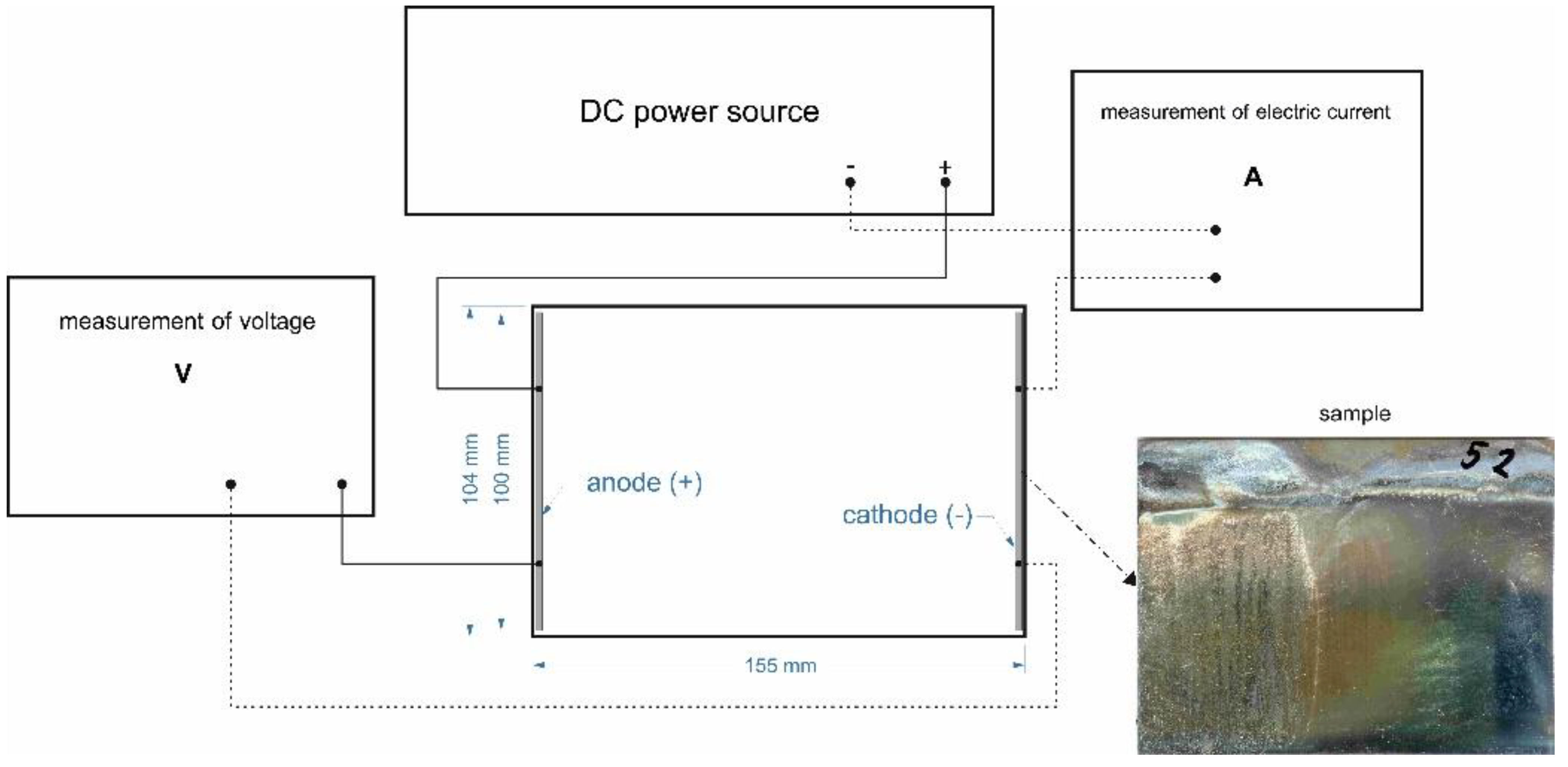
Data intended for further statistical analysis and mathematical modeling in order to achieve our main goals were obtained through an experiment implemented in accordance with the DOE methodology. The schematic plan (wiring diagram) of the experimental apparatus is shown in Figure 1. The selection of factors (and their levels) acting during the experimental procedure must be performed with respect to the theoretical and practical aspects; in our experimental work, both aspects were fulfilled (recommendations of scientific publications and practical experience from engineering practice were taken into account). The individual factor levels are defined in a sense to meet the conditions for the feasibility of the individual experimental runs in all their possible combinations.
Individual experimental samples with dimensions of 100 × 70 × 0.5 mm were pre-treated by chemical degreasing in a 40% NaOH solution at a temperature of 55 °C with a time duration of 10 min. After that, the samples were rinsed in demineralized water at a temperature of 22 °C for 1 min. The experimental samples were subsequently pickled in 20% HCl at a temperature of 20 °C with a time duration of 5 min. The pickled samples were then rinsed in demineralized water at a temperature of 22 °C for 2 min. Samples pre-treated in this way were subjected to electrolytic zinc plating in a slightly acidic electrolyte based on KCl and H3BO3. The setting of the controlled factors of the performed experiment (experimental conditions) is shown in Table 1. In addition to the factors listed in Table 1, the following constant factors were used during the entire experiment for each individual experimental run:
- Anode material zinc with a purity of 99.5%;
- Cathode material: S355J0 (experimental sample);
- The amount of sodium benzoate (C7H5NaO2) in the electrolyte is 5.00 g·L−1;
- Cathode current density J = 2.00 A·dm−2.
In total, 52 separate experiments (experimental runs) were carried out as part of the experimental verification in accordance with the Design of Experiments (DOE) methodology. Practical experience shows that the most suitable type of DOE for the analysis of electrolytic surface treatment processes is the central composite orthogonal design (CCD) [7]. Experimental runs 1–32 represent a full factorial design based on fractional replicates, experiments 43–50 represent the so-called star points of the experiment design, and experiments 53 and 54 represent experiments in the center of the experimental space, the so-called zero points. During the actual implementation of the experiments in accordance with the design matrix, the individual experimental runs were performed in a random order to avoid the subjective preference of one of the factor levels and then minimize the systematic error. After the realization of each separate experiment, the thickness of the formed layer (th) was measured on 5 horizontal and 8 vertical lines. At the intersections of these lines, each measurement was repeated 5 times. Thus, 200 separate measurements of the thickness of the formed layer were performed on each individual sample (individual trial), and a total of 10,400 measurements of the ZC thickness were performed.
3. Results and Discussion
The presented article focuses on the development of a mathematical–statistical nonlinear model predicting the zinc coating thickness, which will allow including the influence of the chemical composition of the electrolyte intended for slight acid electrolytic galvanizing and possible interactions with physical influences (electrolyte temperature, voltage, and time of deposition). Based on the created statistical–mathematical model (based on RSM), this study provides optimal control of the zincing process by determining the optimal values of process parameters to obtain the maximum value of the resulting protective zinc coating subject to considered constraints and technological limitations.
As mentioned above, the thickness of the formed zinc layer represents the basic indicator of the corrosion resistance of the coating. In general, as the thickness of the zinc coating increases, so does its corrosion resistance. Zinc coatings have a priority function of anti-corrosion resistance, and the required thicknesses depend on this. The conclusion of these considerations should be the requirement that the thickness of the created layer is as large as possible. However, we must also consider other limitations that do not allow layers with a relatively large thickness to be created during electrolytic galvanizing. We are initially limited by the very construction of plated parts and their function in assembly units, where the basic dimensional tolerances must be respected so that the surface-treated part can fulfill its function. That is why we mentioned customer requirements in the article. The second important limitation is the ability of the coating to form on the base material by electrocrystallization. Therefore, surfaces with a low value of roughness profile parameters (such as Ra and Rz, which is desirable from the point of view of the quality of the base material) are not able to form coatings with a large thickness. From practical experience, the smaller the value of roughness Ra, the smaller the thickness of the zinc layer must be. With surface roughness smaller than Ra < 0.4 µm, it is already problematic to create a zinc coating. The third basic limitation of the thickness of the zinc layer is the nature of the internal stresses in the formed coating. Since the electrolytically eliminated zinc coatings have internal compressive stresses, cracks and subsequent cracking occur at larger thicknesses (th > 25 µm). Even these basic limitations need to be considered in mutual interaction. Considering the above, it is clear that the essence is not the choice of a specific thickness value but the search for its optimal value (maximum value) within the limiting conditions.
By implementing the first step of the proposed methodology (performed experiment), we obtained results—experimental data in a total number of 10,400 values of the measured thickness of the resulting electrodeposited zinc coating. Taking into account that asymmetric distribution or unconventional variance is a common phenomenon for experimental data, in order to avoid violating the basic requirements imposed on the data set, three sequential steps are implemented during the evaluation: exploratory data analysis (EDA), verification of requirements on a data set and Confirmatory data analysis (CDA) [41]. The samples analysis is focused on determining an objective mean value—a representative value of the results of the measured thickness of zinc layer deposited on individual samples for individual test runs performed at a constant current density of J = 2 [A·dm−2] and, of course, for the measurements on an etalon.
The individual measurements were subjected to evaluation by standard statistical methods. To examine the normality of a data set (values of the thickness of the created zinc layer for each individual sample realized within the experiment), the Shapiro–Wilks test at a level of the significance level of α = 0.05 was employed. The analysis pointed to the fact that all repeated measurements for each individual trial exhibited a Gaussian normal distribution without the presence of gross errors. The identification of the presence of gross errors or outliers and extreme values was analyzed using the Grubbs test criterion and Dixon test. At the same time, repeated measurements at the zero points of the experimental plan (experiment 51 and 52) did not show a significant difference (p = 0.247) based on the Scheffe test at the chosen significance level of 5%. Because of the above-mentioned facts, the objective mean value of each individual experimental run was determined in the form of an arithmetic mean and chosen for further analysis.
3.1. Results of Statistical Analysis of DOE Data and Model Development
We performed statistical analysis of predictive model fitting and validation. Table 2 reports the main statistical characteristics of the developed nonlinear regression model applied to the prediction of the thickness of the formed zinc layer by the electrochemical method. Model diagnostic fit tools, namely, the summary of the fit plot, the lack of fit test, and the normal probability plot of residuals, should be applied to verify the goodness of the developed regression model.
As seen from Table 2, the implemented regression prediction model (16) can explain 95.9403% of the variability of the investigated variable (the response variable—the thickness of the created zinc coating). In other words, the value of the coefficient of determination (also known as R-squared value) is greater than 90% (R2 = 95.9403), and it means that the developed RSM model can adequately describe the behavior of the observed response, which exhibits more regular response behavior. The adjusted coefficient of determination also reaches a high value, up to AdjR2 = 0.944829. As mentioned in [31], if the RSM model provides a high value of AdjR2 (greater than 90%), it is not necessary to use soft computing techniques for modeling technological variables with such way of behavior since they are much more time-consuming when performing computations. In this case, we can talk about functional dependency. The average error of the applied model (16) is 0.609012 μm, and the average value of the thickness of the electrodeposited zinc layer (th) within the entire experiment in 52 individual experimental trials reaches 12.661 μm. Since the value of the R2 alone may not be sufficient to verify the validity of the created model, further analysis was performed.
Table 3 summarises the results of the analysis of variance (ANOVA) for data (ZC thickness) experimentally obtained at the used current density of J = 2 A·dm−2 during the entire experiment. The null statistical hypothesis of the variance analysis includes the statement that none of the factors used in the predictive regression model has a significant effect on the change in the value of the investigated variable (the resulting thickness of the formed zinc layer).
As is observable from the results shown in Table 3, the variability caused by random errors is significantly less than the variability of the values determined and explained by the model. In accordance with the Fisher–Snedecor test criterion, the adequacy of the MSNm is indicated by the achieved value of p (<0.0001), which is less than the chosen level of significance α = 0.05. Based on the statistical hypothesis verification, it is possible to conclude that we do not have enough evidence to accept the null statistical hypothesis, and therefore, we can consider the applied regression model as adequate. This means that at the chosen level of significance α = 0.05, there is at least one significant parameter (factor) in the developed model which affects the value of th—the thickness of the formed zinc layer. To evaluate the model’s validity and diagnose its predictive power (if well fits the observed experimental data), the residual variability should be compared with the variability of measured data within groups. For this purpose, the ANOVA lack-of-fit test was used, and verification of the null statistical hypothesis (H0 claims that the variance of the residuals is less than or equal to the variance within the groups) was tested against the alternative hypothesis HA at the chosen confidence interval of α = 0.05. The alternative hypothesis HA claims that the variance of residuals is greater than the variance within groups. The outputs of the ANOVA lack-of-fit test are presented in Table 4.
Based on the achieved value p = 0.4264 of the Fisher test criterion converted to a probability scale, it is possible to state that we do not have enough evidence to reject the null statistical hypothesis (H0). Hence, the result is that the variance of the residuals is less than or equal to the variance of the values within the groups, and thus the regression model sufficiently describes the investigated dependence. In other words, the model exhibits a good fit to the data (as in our case, sufficiently low model error is obtained), and we can conclude that the developed MSNm (14) is statistically correct and adequate. The presence or absence of main effects and an interaction effect also have been investigated mathematically by the hypothesis testing problem.
Taking into account that the developed model (14) passes the basic assumptions required from such a model and fulfills the basic statistical diagnostic (Table 3 and Table 4), we perform the last stage in the statistical analysis of DOE data—the estimation of unknown model coefficients/parameters. In Table 5, we present the estimation of individual regression coefficients, including testing of their statistical significance and the estimation of Variance Inflation Factors (VIF). The regression coefficients of the model MSNm are reported in Table 5 in column “Estimate” in order from the highest impact to the lowest. They are unscaled here (they are listed in the coded unit here) but refer to the original measurement scale of the considered explanatory variables listed in Table 1.
Based on the estimation of the model parameters (shown in Table 5), it was possible to express the dependence of the response variable (th—the ZC thickness) on the explanatory variables x1—x8 and compile the mathematical–statistical nonlinear model (14) (MSNm) including statistically significant factors and also statistically significant interactions of these factors. When using coded input variables, the fitted model can be written as follows:
The applied regression model (14) represents the best solution, which satisfies theoretical laws, and, at the same time, during its subsequent verification in laboratory and production conditions, it produces errors in the results between the calculated and actual measured value of ± 5%. However, if we additionally look at the influence of the most significant interactions in the sense of Table 5, removing the interactions from (14) causes a drop in the value of the correlation coefficient to 0.891848 and the value of the adjusted coefficient of determination to 0.856699. Removing the second significant interaction from model (14) causes the correlation coefficient to drop to 0.941235 and the adjusted coefficient of determination to 0.922136. By removing the influence of the third power of the deposition time from model (14), the correlation coefficient drops to the value of 0.936665 and the adjusted coefficient of determination to 0.91608. A similar change will occur when the interaction is removed from (14). Changing model (14) by removing all interactions would cause a decrease in the value of the correlation coefficient to 0.777234 and the value of the AdjR2 to a value of 0.763868. In practical application, due to the increasing accuracy of the production of machine parts, it is necessary to ensure the smallest possible deviation of the actual thickness of the created layer from the thickness defined in the technical documentation. Therefore, it is necessary to create a functional model for predicting the thickness of the zinc layer in this area as well, which will show the smallest possible error. Other polynomials were also analyzed, but based on the results mentioned above, the used model (14) was chosen as the most suitable model.
In order to compile the appropriate shape of the prediction model for engineering practice, the developed model (MSNm) would reflect the natural scale of the individual explanatory variables (predictors). Therefore, it is necessary to remember that during the analysis of the experimentally obtained results (data), the individual predictors (factors) were considered in a coded scale, coded by DOE standardization using the well-known formula:
where xd(i) is the standardized variable according to DoE, x(i) is the original main source, while i = 1, 2, …, n and n is the number of basic factors, xmax is the maximum value of the original variable x(i) and xmin is the minimum value of the original variable x(i). Considering the transfer relation (15) and mathematical–statistical formula of the fitted model (14), it is possible to compile the computational model (MSNm) on natural scale, describing the dependence of the investigated variable th on the chemical and physical factors operating during acid galvanizing for the used current density of J = 2 A·dm−2, as follows:
For the complexity of the performed analysis and confirmation of the correctness and suitability of the selected model, it is still necessary to verify the residuals, that is, the difference between the actual measured and predicted values, calculated using the prediction model (16), specifically from the view of their distribution and autocorrelation. The value of the Durbin–Watson autocorrelation test DW = 2.0333681 (p = 0.5933) enables us to accept the null statistical hypothesis of the absence of autocorrelation, and the achieved significance level of the Shapiro–Wilks test (p = 0.0533) points to the Gaussian distribution of the residuals, which reach a mean value of 7.78·10−11 [μm]. In conclusion, we can proclaim the prediction model as statistically and numerically correct.
It is clear from Table 5 that the absolute term of the model (Intercept x0) has the highest effect on the variability of the response (the zinc coating thickness). Intercept represents both all unconsidered input variables operating during the zincing process and applied intervals of considered covariates. Based on the estimation of the regression coefficients (Table 5) of the developed models (14) and (16), it can be seen that the deposition time (td) is the most significant explanatory variable (predictor x7) affecting the resulting thickness of the formed zinc layer. The deposition time appears in the model as the main effect and contributes 22.627% to the changes in the layer thickness. The second most important parameter of the model (16), affecting the changes in the thickness of the electrodeposited layer, is the amount of zinc in the electrolyte, expressed as the amount of ZnCl2 (x1). The amount of ZnCl2 in the electrolyte contributes 10.121% as a main effect and 12.086% as a square effect to the change in layer thickness. The influence of these two most significant parameters of the model (16) on the ZC thickness is shown in Figure 2.
The obtained results are in accordance with the theory of the formation of zinc layers [38,47]. If we consider the influence of only the main effects, these conclusions follow from the theory of electrolytic deposition of zinc coatings [47]. Although the theory says that by increasing the deposition time, the thickness of the created layer increases too, in the real process, it is also necessary to consider the mutual interaction of the deposition time and other physical and chemical factors acting during the process. From the chemical factors, it is precisely the amount of zinc in the electrolyte that affects the polarization phenomena [38,47,48]. At the same time, it is necessary to point out the fact that with increasing the deposition time, the amount of zinc decreases in the electrolyte. Then, the previous statement is valid, but with a certain limitation. The growth of the thickness due to the increase in deposition time is valid only for the amount of ZnCl2 higher than 45 gL−1.
Let us examine the interrelationship and interaction of deposition time td and amount of ZnCl2. The interaction of the deposition time and the amount of ZnCl2 (x7·x1) occurs in the model with a 3.974% share, and the interaction of the squared value of the deposition time and the amount of ZnCl2 (x7· x7·x1) occurs in the model with a share of 3.119%. It is clear from this that as the deposition time td increases and the concentration of ZnCl2 in the electrolyte increases too, the thickness of the formed layer (th) also (nonlinearly) increases.
This increase in the thickness of the zinc layer due to the increase in the amount of ZnCl2 (x7) in the electrolyte is primarily caused by a decrease in the concentration and chemical polarization of the cathode.
Other significant factors (considered as the main effect of factor at the chosen significance level of α = 0.05, which affect the thickness of the formed zinc coating) are the temperature of the electrolyte TE (x6) with a share of 8.217% and the amount of KCl (x3) in the electrolyte with a 6.583% influence. The interaction of the electrolyte temperature and the deposition time (x7·x6) with a 6.268% share in the change of the ZC thickness is interesting for researchers in surface engineering, as well as the interaction of the amount of ZnCl2 and the basic gloss-forming additive BA (x1·x4) with a 5.968% share in the changes in the investigated thickness of the created layer.
The validity of the model (16) created by nonlinear regression analysis compared to the theoretical model (6) derived from Faraday’s laws is documented in Figure 2.
First of all, it is necessary to mention the fact that the average deviation of the actually measured layer thickness and the layer thickness calculated by the regression model (16) for all experiments (52 individual experiments in terms of the established experimental plan) represents only −0.193%. On the other hand, the average deviation between the actually measured layer thickness and the layer thickness calculated by the theoretical model (6) represents 64.156%. This significant difference is primarily caused by a more complex description of the real dependencies of the technological process of electrolytic galvanizing between chemical and physical factors expressed by the regression model (16). This fact confirms and justifies the use of the created model (16) in practice, which describes the dependence of the thickness of the created layer on the change of chemical and physical factors in the sense of Table 1.
3.2. Results of the Optimization Procedure
When optimizing a technological process, it is possible to consider several criteria; most often, the economic and qualitative aspects are taken into account. This is also the case when optimizing the galvanizing process. In accordance with the mathematical theory of optimal decision-making [43,44,45,49,50,51,52,53,54] applied to the solution of practical engineering problems, it is necessary to have available (a) a mathematical model of the process/system that we want to optimize; (b) objective function and (c) constraints. As we mentioned above (in Section 2.2.2), the engineering optimization problem (EOP) presented in this paper involves one objective—maximization of the thickness of the formed zinc coating in the sense of “higher value of ZC thickness increases the protective properties of treated steel parts” and contains a finite number of inequality constraints defining a feasible region X. In other words, we consider EOP: where is the objective function and represent the feasible region. On the basis of the developed mathematical–statistical nonlinear model (16), it is possible to perform the optimization procedure of the acid zinc plating process. We will present a more specific form of the objective function only after determining the limiting conditions that we must take into account. Therefore, let us take a closer look at the economic and qualitative aspects that result in the boundaries for EOP.
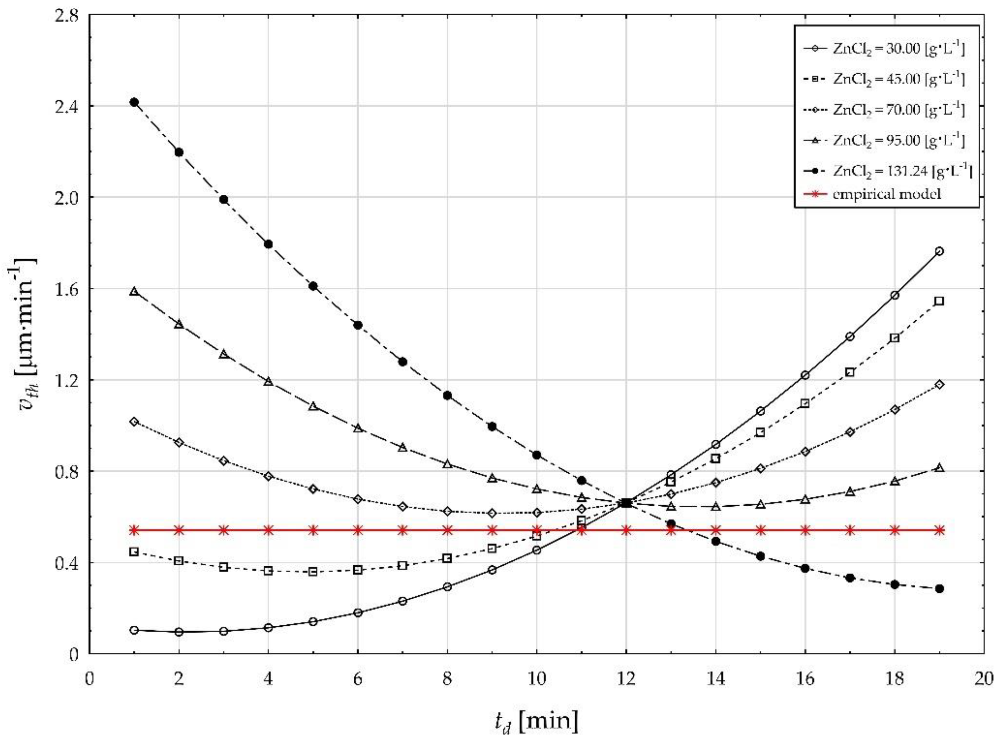
From an economic point of view, the rate of layer deposition is a very interesting and important parameter in the technological processes of electrolytic formation of coatings. If we consider model (16) to be correct and adequate for predicting the thickness of the formed layer, then the rate of zinc excretion from the weakly acidic galvanizing electrolyte can be determined as the first derivative of the function (16) with respect to time, that is, the deposition time td. In this case, we can write a function in the form (17) for the zinc coating excretion rate:
Formula (17) expresses the rate of zinc coating deposition (Figure 3) from the slightly acidic galvanizing electrolyte primarily affects the quality of the deposited layer. From an economic point of view, it is, of course, advantageous if the rate of deposition is as high as possible. Then, we can create a layer of the required thickness in the shortest possible time. However, the rate of layer formation affects the very course of electro crystallization, and therefore it is not suitable from the point of view of the quality of the excluded layer if this rate exceeds 1.50 μm·min−1.
However, from an economic point of view, it is not suitable for the speed of layer formation to be lower than 0.60 μm·min−1. The relationship (17), describing the rate of formation of the zinc layer (Figure 3), points to the fact that the rate of formation of the layer is not constant, as presented by the empirical relationship. Theoretical model (6) considers only the theoretical rate of formation of the layer (0.285 μm·min−1), current yield (95%), and actual used current density (2 A·dm−2). The compiled model (16) takes into account the amount of zinc in the electrolyte, which is expressed in the amount of ZnCl2, the temperature of the electrolyte (TE), the deposition time (td), and the amount of the main gloss-forming additive in the electrolyte (MBA), including their mutual interactions, when determining the rate of zinc coating formation. We use the above-mentioned facts from the point of view of the quality of the created layer and the economy of the process of electrolytic deposition of the zinc coating itself in the following part as limitations during optimization.
In general, the corrosion resistance of zinc coatings is directly proportional to their thickness (th). This means that in order to achieve the highest possible corrosion resistance, the thickness of the created layer must be as large as possible. Of course, there are limitations given by the very condition of the surface of the plated structural component, primarily the roughness of the surface, limitations given by the internal stresses in the created layer, which create an upper limit of the layer thickness beyond which it is no longer technologically possible to go. Based on the previous conclusions about the numerical and statistical correctness of the model (16) developed to predict the thickness th of the formed zinc coating when considering eight explanatory variables x1, x2, …, x8, the regression model (16) can be accepted as a valid mathematical–statistical model and useful for the next optimization procedure. The optimality criterion should take into account the aspect of economic efficiency of the zincing process. Practical experience exhibits that up to 91% of customers define the thickness of the protective layer as a basic requirement for galvanizing surface treatment; it is the most frequently specified parameter in the project documentation. When considering the intervals of the variables used in the experimental verification, as well as the limitations given by the speed of the created layer, then the basic limitations for the process of nonlinear optimization are:
where vth represents relation (15).
The regression model (16) was chosen as the objective function for the nonlinear optimization of the thickness of the formed zinc layer.
In accordance with the explanatory variables listed in the natural scale in Table 1, the considered engineering optimization problem (EOP) can be written as follows:
subject to the constraints (18), where th is defined by MSNm (16).
The graphical outputs of the optimization process conducted in the MATLAB software environment are given in Figure 4. Our main goal was to find such a combination of considered parameters in (19) from a feasible region, which will guarantee the maximum value of the objective function while complying with all prescribed technological limitations. This combination of numbers symbolizes the optimal solution.
To solve the defined EOP, searching for the maximum value of the objective function (19) subject to the defined optimization constraints (18), an appropriate script was created in MATLAB 2019a software. Nonlinear programming (NP) methods available within the Optimisation toolbox were used, specifically the “fmincon ()” solver for constrained nonlinear minimization and the interior point method (IPM) algorithm.
Based on the performed nonlinear optimization procedure, the optimal value (th*) of the thickness of the formed zinc layer was determined. Specifically, we obtained the optimum as th* = 12.7036 μm at the following optimal combination of values of the control parameters considered in (19) at an applied current density of J = 2 A·dm−2:
m(ZnCl2) = 61.24 g· L−1, m(H3BO3) = 24.49 g ·L−1, m(KCl) = 171.46 g ·L−1,
m(BA) = 36.74 mL·L−1, m(MBA) = 2.45 mL·L−1, TE = 24.49 °C, td = 9.80 min and U = 2.45 V.
These results were verified under real operating conditions. As mentioned above, the limiting conditions derive from practical experience and requirements of related research works.
4. Conclusions
In recent years, the effort of researchers to find the right combination of input variables and their values for certain technological processes is evident. The same can be said about improving the galvanizing process. In order to fulfill these efforts, it has become necessary to apply the methods of applied mathematics to a greater extent. It is important to use the options currently offered: methods of modern applied mathematics, experimentation in accordance with the DOE methodology, methods of multivariate statistical analysis, and optimization methods in connection with advances in computing technology and special software. This article is a confirmation of the usefulness of the implementation of the above-mentioned areas of mathematics. Thanks to the experiment carried out with regard to the DOE approach, we obtained DOE data. Based on the statistical analysis of experimentally obtained DOE data, the mathematical–statistical nonlinear model (16) predicting the thickness of the created protective zinc coating was developed, the coefficient of the determination reached the value of R2 = 0.959403, and the adjusted coefficient of the determination reached the value of AdjR2 = 0.944829.
The results obtained in this research study demonstrate the significance of the influence of certain explanatory variables on the thickness of the zinc coating (created at the current density J = 2 A·dm−2 used in the practice of surface engineering) not only in the role as a main effect but also in interactions, e.g., time of depositions td (x7) and the amount of ZnCl2 (x1) in the electrolyte.
The research study proclaims the usefulness of the application of mathematical modeling in combination with optimization methods in efforts to control technological processes. The optimization procedure was based on the developed regression model. The combination of optimal values of the input factors acting during acid galvanizing was determined. The goal of the optimization procedure—to achieve the maximum thickness of the resulting zinc coating under the defined limitations given by the technological limitations of the acid galvanizing process—was achieved, and the resulting thickness with a value of th* = 12.7036 μm was obtained. It is worth noting here that experimentation in conjunction with optimization is important; it must go hand in hand. Without experimentation, we cannot optimize (as it is necessary to develop an adequate mathematical model), and experimenting without striving to optimize the technological process is not worthwhile.
By implementing the developed regression model (16) into the practice of surface engineering, it was possible to eliminate uncertainties in the technological response (zinc coating thickness) of the galvanizing process in a slight acid bath. We have created a strategy to solve a practical problem that arises when creating zinc layers by the electrolytic method. This procedure/strategy, summarized in points/steps (i)–(iv) within Section 2.2, has also been applied to other surface treatment processes such as anodic aluminum oxidation, electrolytic nickel plating, electrolytic tin plating, electrolytic zinc plating in alkaline electrolytes and currently, is working on an application for cataphoretic painting. We have been developing this procedure for several years in cooperation with practice and for the needs of a private company whose main task is the implementation of electrolytic surface treatments. Based on the model (16) and its subsequent verification in the practical conditions of the production process, the private company managed to be able to achieve the required thickness of the layers with high precision and within relatively narrow tolerances. This is also interesting for the company from an economic point of view and from the point of view of quality.
For further investigation in this research field, it will be necessary to take a more comprehensive approach to optimization. To achieve an appropriate zinc layer under optimal process conditions, we must also take into account the value of the critical temperature. In the future, we want to focus our attention on experimental and research activities on the analysis of the zinc layer formation based on machine learning and methods of artificial intelligence.
Funding
This research received no external funding.
Data Availability Statement
Not applicable.
Conflicts of Interest
The author declares no conflict of interest.
References
- Jędrzejczyk, D.; Szatkowska, E. The Impact of Heat Treatment on the Behavior of a Hot-Dip Zinc Coating Applied to Steel During Dry Friction. Materials 2021, 14, 660. [Google Scholar] [CrossRef]
- Klekotka, M.; Zielińska, K.; Stankiewicz, A.; Kuciej, M. Tribological and Anticorrosion Performance of Electroplated Zinc Based Nanocomposite Coatings. Coatings 2020, 10, 594. [Google Scholar] [CrossRef]
- Kavitha, B.; Santhosh, P.; Renukadevi, M.; Kalpana, A.; Shakkthivel, P.; Vasudevan, T. Role of organic additives on zinc plating. Surf. Coat. Technol. 2006, 201, 3438–3442. [Google Scholar] [CrossRef]
- Zhang, X.G.; Valeriote, E.M. Galvanic protection of steel and galvanic corrosion of zinc under thin layer electrolytes. Corros. Sci. 1993, 34, 1957–1972. [Google Scholar] [CrossRef]
- Boshkov, N.; Petrov, K.; Kovacheva, D.; Vitkova, S.; Nemska, S. Influence of the alloying component on the protective ability of some zinc galvanic coatings. Electrochim. Acta 2005, 51, 77–84. [Google Scholar] [CrossRef]
- Yadav, A.P.; Katayama, H.; Noda, K.; Masuda, H.; Nishikata, A.; Tsuru, T. Effect of Al on the galvanic ability of Zn–Al coating under thin layer of electrolyte. Electrochim. Acta 2007, 52, 2411–2422. [Google Scholar] [CrossRef]
- Badida, M.; Sobotova, L.; Gombar, M.; Kmec, J.; Kucerka, D.; Hrmo, R. The contribution to coating quality evaluation by statistical methods. Metalurgija 2016, 55, 445–448. [Google Scholar]
- Yadav, A.P.; Katayama, H.; Noda, K.; Masuda, H.; Nishikata, A.; Tsuru, T. Surface potential distribution over a zinc/steel galvanic couple corroding under thin layer of electrolyte. Electrochim. Acta 2007, 52, 3121–3129. [Google Scholar] [CrossRef]
- Jong-Min, L. Numerical analysis of galvanic corrosion of Zn/Fe interface beneath a thin electrolyte. Electrochim. Acta 2006, 51, 3256–3260. [Google Scholar] [CrossRef]
- Dubent, S.; Mertens, M.L.A.D.; Saurat, M. Electrodeposition, characterization and corrosion behaviour of tin–20wt.% zinc coatings electroplated from a non-cyanide alkaline bath. Mater. Chem. Phys. 2010, 120, 371–380. [Google Scholar] [CrossRef]
- Maniam, K.K.; Paul, S. Progress in Electrodeposition of Zinc and Zinc Nickel Alloys Using Ionic Liquids. Appl. Sci. 2020, 10, 5321. [Google Scholar] [CrossRef]
- Wang, Y. Study on Influence Factors of zinc layer thickness via Response Surface Method, Taguchi Method and Genetic Algorithm. Ind. Eng. Manag. 2018, 07, 1000245. [Google Scholar] [CrossRef]
- Luis Pérez, C.J. A Proposal of an Adaptive Neuro-Fuzzy Inference System for Modeling Experimental Data in Manufacturing Engineering. Mathematics 2020, 8, 1390. [Google Scholar] [CrossRef]
- Dobránsky, J.; Gombár, M.; Stejskal, T. The Influence of the Use of Technological Waste and the Simulation of Material Lifetime on the Unnotched Impact Strength of Two Different Polymer Composites. Materials 2022, 15, 8516. [Google Scholar] [CrossRef] [PubMed]
- Oniszczuk-Świercz, D.; Świercz, R.; Michna, Š. Evaluation of Prediction Models of the Microwire EDM Process of Inconel 718 Using ANN and RSM Methods. Materials 2022, 15, 8317. [Google Scholar] [CrossRef]
- Valíček, J.; Czán, A.; Harničárová, M.; Šajgalík, M.; Kušnerová, M.; Czánová, T.; Kopal, I.; Gombár, M.; Kmec, J.; Šafář, M. A new way of identifying, predicting and regulating residual stress after chip-forming machining. Int. J. Mech. Sci. 2019, 155, 343–359. [Google Scholar] [CrossRef]
- Świercz, R.; Oniszczuk-Świercz, D.; Chmielewski, T. Multi-Response Optimization of Electrical Discharge Machining Using the Desirability Function. Micromachines 2019, 10, 72. [Google Scholar] [CrossRef]
- Hrehová, S. Possibilities of Data Analysis Using Data Model. In Proceedings of the 4th EAI International Conference on Management of Manufacturing System (MMS 2019), Krynica Zdroj, Poland, 8–10 October 2019; EAI/Springer Innovations in Communication and Computing. Springer: Cham, Switzerland, 2019. [Google Scholar] [CrossRef]
- Hoskova-Mayerova, S.; Kalvoda, J.; Bauer, M.; Rackova, P. Development of a Methodology for Assessing Workload within the Air Traffic Control Environment in the Czech Republic. Sustainability 2022, 14, 7858. [Google Scholar] [CrossRef]
- Bekesiene, S.; Samoilenko, I.; Nikitin, A.; Meidute-Kavaliauskiene, I. The Complex Systems for Conflict Interaction Modelling to Describe a Non-Trivial Epidemiological Situation. Mathematics 2022, 10, 537. [Google Scholar] [CrossRef]
- Panda, A.; Zaloga, V.; Dyadyura, K.; Rybalka, I.; Pandova, I. Modelling Business Process of Manufacturing for Air Compressors. TEM J. 2019, 8, 430–436. [Google Scholar] [CrossRef]
- Sánchez, L.; Leiva, V.; Saulo, H.; Marchant, C.; Sarabia, J.M. A New Quantile Regression Model and Its Diagnostic Analytics for a Weibull Distributed Response with Applications. Mathematics 2021, 9, 2768. [Google Scholar] [CrossRef]
- Anand, V.; Srivastava, V.C. Zinc oxide nanoparticles synthesis by electrochemical method: Optimization of parameters for maximization of productivity and characterization. J. Alloy. Compd. 2015, 636, 288–292. [Google Scholar] [CrossRef]
- Dhak, D.; Mahon, M.; Asselin, E.; Alfantazi, A. Characterizing industrially electrowon sticky zinc deposits. Hydrometallurgy 2012, 111–112, 136–140. [Google Scholar] [CrossRef]
- Aliofkhazraei, M.; Alamdari, E.K.; Zamanzade, M.; Salasi, M.; Behrouzghaemi, S.; Heydari, J.; Haghshenas, D.F.; Zolala, V. Empirical equations for electrical conductivity and density of Zn, Cd and Mn sulphate solutions in the range of electrowinning and electrorefining electrolytes. J. Mater. Sci. 2007, 42, 9622–9631. [Google Scholar] [CrossRef]
- Yu, J.; Wang, L.; Su, L.; Ai, X.; Yang, H. Temperature Effects on the Electrodeposition of Zinc. J. Electrochem. Soc. 2002, 150, C19–C23. [Google Scholar] [CrossRef]
- Jedrzejczyk, D. Effect of High Temperature Oxidation on Structure and Corrosion Resistance of the Zinc Coating Deposited on Cast Iron. Arch. Met. Mater. 2012, 57, 145–154. [Google Scholar] [CrossRef]
- Xia, X.; Zhitomirsky, I.; McDermid, J.R. Electrodeposition of zinc and composite zinc–yttria stabilized zirconia coatings. J. Mater. Process. Technol. 2009, 209, 2632–2640. [Google Scholar] [CrossRef]
- Alfantazi, A.M.; Dreisinger, D. The role of zinc and sulfuric acid concentrations on zinc electrowinning from industrial sulfate based electrolyte. J. Appl. Electrochem. 2001, 31, 641–646. [Google Scholar] [CrossRef]
- Kania, H.; Mendala, J.; Kozuba, J.; Saternus, M. Development of Bath Chemical Composition for Batch Hot-Dip Galvanizing—A Review. Materials 2020, 13, 4168. [Google Scholar] [CrossRef]
- Mackinnon, D.J.; Brannen, J.M.; Fenn, P.L. Characterization of impurity effects in zinc electrowinning from industrial acid sulphate electrolyte. J. Appl. Electrochem. 1987, 17, 1129–1143. [Google Scholar] [CrossRef]
- Verma, N.; Sharma, V.; Badar, M.A. Improving sigma level of galvanization process by zinc over-coating reduction using an integrated Six Sigma and design-of-experiments approach. Arab. J. Sci. Eng. 2022, 47, 8535–8549. [Google Scholar] [CrossRef]
- Bennasr, J.; Snoussi, A.; Bradai, C.; Halouani, F. Optimization of hot-dip galvanizing process of reactive steels: Minimizing zinc consumption without alloy additions. Mater. Lett. 2008, 62, 3328–3330. [Google Scholar] [CrossRef]
- Lorza, R.L.; Calvo, M.Á.M.; Labari, C.B.; Fuente, P.J.R. Using the Multi-Response Method with Desirability Functions to Optimize the Zinc Electroplating of Steel Screws. Metals 2018, 8, 711. [Google Scholar] [CrossRef]
- Vagaská, A.; Gombár, M.; Kmec, J.; Michal, P. Statistical Analysis of the Factors Effect on the Zinc Coating Thickness. Appl. Mech. Mater. 2013, 378, 184–189. [Google Scholar] [CrossRef]
- Michal, P.; Gombár, M.; Vagaská, A.; Piteľ, J.; Kmec, J. Experimental Study and Modeling of the Zinc Coating Thickness. Adv. Mater. Res. 2013, 712–715, 382–386. [Google Scholar] [CrossRef]
- Michal, P.; Piteľ, J.; Vagaská, A.; Bukovský, I. Application of neural networks to evaluate experimental data of galvanic zincing. In Proceedings of the 2014 International Joint Conference on Neural Networks (IJCNN), Beijing, China, 6–11 July 2014; IEEE: New York, NY, USA, 2014; pp. 2997–3001. [Google Scholar]
- Bartl, D.O.; Mudroch, O. Technologie Chemických a Elektrochemických Povrchových Úprav I, 1st ed.; SNTL: Prague, Czech Republic, 1957; p. 448. [Google Scholar]
- Hayter, A. Probability and Statistics for Engineers and Scientists, 4th ed.; Thomson Brooks/Cole, Cengage Learning: Toronto, ON, Canada, 2013; p. 826. [Google Scholar]
- Box, G.E.P.; Hunter, J.S.; Hunter, W.G. Statistics for Experimenters. Design, Innovation, and Discovery, 2nd ed.; John Wiley & Sons: Hoboken, NJ, USA, 2005; p. 639. [Google Scholar]
- Vagaská, A.; Gombár, M.; Straka, Ľ. Selected Mathematical Optimization Methods for Solving Problems of Engineering Practice. Energies 2022, 15, 2205. [Google Scholar] [CrossRef]
- Hatefi, E.; Hatefi, A. Estimation of Critical Collapse Solutions to Black Holes with Nonlinear Statistical Models. Mathematics 2022, 10, 4537. [Google Scholar] [CrossRef]
- Yang, W.Y.; Cao, W.; Chung, T.S.; Morris, J. Applied Numerical Methods Using MATLAB; John Wiley & Sons, Inc.: Hoboken, NJ, USA, 2005; p. 509. [Google Scholar]
- Camacho, E.F.; Alba, C.B. Model Predictive Control, 2nd ed.; Springer Science & Business Media: New York, NY, USA, 2013; pp. 249–287+427. [Google Scholar]
- Hamala, M.; Trnovská, M. Nelineárne Programovanie/Nonlinear Programming; Epos: Bratislava, Slovak Republic, 2012; p. 339. [Google Scholar]
- Behún, M.; Knežo, D.; Cehlár, M.; Knapčíková, L.; Behúnová, A. Recent Application of Dijkstra’s Algorithm in the Process of Production Planning. Appl. Sci. 2022, 12, 7088. [Google Scholar] [CrossRef]
- Ruml, V. Abeceda Povrchových Úprav Kovov, 1st ed.; PRÁCE: Prague, Czech Republic, 1956; p. 175. [Google Scholar]
- Ruml, V.; Soukup, M. Galvanické Pokovování, 1st ed.; SNTL: Prague, Czech Republic, 1981; p. 324. [Google Scholar]
- Rao, S. Engineering Optimization. Theory and Practice, 4th ed.; John Wiley & Sons, Inc.: Hoboken, NJ, USA, 2009; p. 830. [Google Scholar]
- Antoniou, A.; Lu, W.S. Practical Optimization. Algorithms and Engineering Applications; Springer Science & Business Media LCC: New York, NY, USA, 2007; pp. 547–558+675. [Google Scholar]
- Boyd, S.; Vandenberghe, L. Convex Optimization; Cambridge University Press: Cambridge, UK, 2009; 701p. [Google Scholar]
- Belegundu, A.D.; Chandrupatla, T.R. Optimization Concepts and Applications in Engineering; Cambridge University Press: Cambridge, UK, 2011. [Google Scholar] [CrossRef]
- Bakare, E.A.; Hoskova-Mayerova, S. Optimal Control Analysis of Cholera Dynamics in the Presence of Asymptotic Transmission. Axioms 2021, 10, 60. [Google Scholar] [CrossRef]
- Coronado de Koster, O.A.; Domínguez-Navarro, J.A. Multi-Objective Tabu Search for the Location and Sizing of Multiple Types of FACTS and DG in Electrical Networks. Energies 2020, 13, 2722. [Google Scholar] [CrossRef]
Figure 1.
Connection diagram of the experimental apparatus.

Figure 2.
Graphical representation of the thickness of the resulting zinc coating formed during acid zinc plating for theoretical model (6)—plotted in red color; and for developed nonlinear regression model (16).
Figure 2.
Graphical representation of the thickness of the resulting zinc coating formed during acid zinc plating for theoretical model (6)—plotted in red color; and for developed nonlinear regression model (16).

Figure 3.
The graphical presentation of dependences in the speed of zinc coating growth on the time of deposition at defined amount of zinc chloride in the electrolyte.
Figure 3.
The graphical presentation of dependences in the speed of zinc coating growth on the time of deposition at defined amount of zinc chloride in the electrolyte.

Figure 4.
Graphical outputs of the optimization procedure for the required ZC thickness.


Table 1.
Levels of factors (explanatory variables) used during the experiment.
| Factor (Code) | Factor (Natural) | Factor Unit | Factor Level | ||||
|---|---|---|---|---|---|---|---|
| −2.449 | −1 | 0 | +1 | +2.449 | |||
| x1 | ZnCl2 | g·L−1 | 8.76 | 45.00 | 70.00 | 95.00 | 131.24 |
| x2 | H3BO3 | g·L−1 | 5.51 | 20.00 | 30.00 | 40.00 | 54.49 |
| x3 | KCl | g·L−1 | 3.54 | 105.00 | 175.00 | 245.00 | 346.46 |
| x4 | BA | ml·L−1 | 3.26 | 25.00 | 40.00 | 60.00 | 76.74 |
| x5 | MBA | ml·L−1 | 0.55 | 2.00 | 3.00 | 4.00 | 5.45 |
| x6 | TE | °C | −2.49 | 12.00 | 22.00 | 32.00 | 46.49 |
| x7 | td | min | 0.20 | 6.00 | 10.00 | 14.00 | 19.80 |
| x8 | U | V | 1.55 | 3.00 | 4.00 | 5.00 | 6.45 |
The factors represent ZnCl2—zinc chloride, H3BO3—boric acid, KCl—potassium chloride, BA—brightener additive, MBA—main brightener additive, TE—electrolyte temperature, td—time of deposition, U—voltage.
Table 2.
The summary statistics of the nonlinear regression model of the layer thickness (th).
| Parameter | Value |
|---|---|
| RSquare | 0.959403 |
| RSquare Adj | 0.944829 |
| Root Mean Square Error | 0.609012 |
| Mean of Response | 12.66074 |
| Observations (or Sum Wgts) | 54 |
Table 3.
ANOVA evaluation of the regression model (MSNm) of the layer thickness (th).
| Source | df | Sum of Squares | Mean Square | F Ratio | p |
|---|---|---|---|---|---|
| Model | 14 | 341.8378 | 24.417 | 65.8324 | <0.0001 * |
| Error | 39 | 14.46495 | 0.3709 | ||
| C. Total | 53 | 356.3028 |
*—significant at significance level of α = 0.05. Source: Compiled and calculated by the authors using Statistica 13.5, Matlab2019b, and JPM 11.
Table 4.
Lack of Fit for a nonlinear model of the layer thickness (th).
| Source | df | Sum of Squares | Mean Square | F Ratio | p |
|---|---|---|---|---|---|
| Lack Of Fit | 36 | 13.69565 | 0.380435 | 1.4836 | 0.4264 |
| Pure Error | 3 | 0.7693 | 0.256433 | ||
| Total Error | 39 | 14.46495 |
Table 5.
The estimation of regression coefficients of the developed nonlinear model predicting the zinc coating thickness (th).
Table 5.
The estimation of regression coefficients of the developed nonlinear model predicting the zinc coating thickness (th).
| Term | Estimate | Std Error | t Ratio | Prob>|t| | −95% CI | +95% CI | VIF |
|---|---|---|---|---|---|---|---|
| Intercept | 13.20027 | 0.106555 | 123.88 | <0.0001 * | 12.98474 | 13.4158 | . |
| x7 | 1.999702 | 0.132512 | 15.09 | <0.0001 * | 1.731672 | 2.267732 | 2.272463 |
| x1 | 1.185961 | 0.175807 | 6.75 | <0.0001 * | 0.830359 | 1.541564 | 1.999999 |
| x6 | 0.536572 | 0.097868 | 5.48 | <0.0001 * | 0.338615 | 0.734528 | 1.239563 |
| x3 | 0.411504 | 0.093711 | 4.39 | <0.0001 * | 0.221954 | 0.601053 | 1.136512 |
| x7·x1 | 0.282726 | 0.106549 | 2.65 | 0.0115 * | 0.06721 | 0.498243 | 1.101924 |
| x1·x1 | −0.60697 | 0.075346 | −8.06 | <0.0001 * | −0.75937 | −0.45457 | 1.000000 |
| x7·x6 | 0.438066 | 0.104858 | 4.18 | 0.0002 * | 0.225971 | 0.650162 | 1.067221 |
| x3·x8 | 0.275512 | 0.125774 | 2.19 | 0.0345 * | 0.021109 | 0.529915 | 1.535445 |
| x7·x5 | 0.40297 | 0.114282 | 3.53 | 0.0011 * | 0.171812 | 0.634128 | 1.267674 |
| x3·x5 | −0.29171 | 0.107228 | −2.72 | 0.0097 * | −0.50859 | −0.07482 | 1.115997 |
| x1·x4 | −0.46195 | 0.116077 | −3.98 | 0.0003 * | −0.69674 | −0.22716 | 1.307807 |
| x6·x4 | 0.324827 | 0.128789 | 2.52 | 0.0159 * | 0.064326 | 0.585328 | 1.609937 |
| x7·x7·x7 | 0.126336 | 0.041106 | 3.07 | 0.0039 * | 0.04319 | 0.209481 | 1.132125 |
| x7·x7·x1 | −0.44179 | 0.212534 | −2.08 | 0.0443 * | −0.87168 | −0.0119 | 1.384377 |
x1—ZnCl2, x2—H3BO3, x3—KCl, x4—BA, x5—MBA, x6—TE, x7—td, x8—U, *—significant at the chosen level of α = 0.05. Source: Compiled by the authors using Statistica 13.5, Matlab2019b, and JPM 11.
Disclaimer/Publisher’s Note: The statements, opinions and data contained in all publications are solely those of the individual author(s) and contributor(s) and not of MDPI and/or the editor(s). MDPI and/or the editor(s) disclaim responsibility for any injury to people or property resulting from any ideas, methods, instructions or products referred to in the content. |
© 2023 by the author. Licensee MDPI, Basel, Switzerland. This article is an open access article distributed under the terms and conditions of the Creative Commons Attribution (CC BY) license (https://creativecommons.org/licenses/by/4.0/).
Share and Cite
MDPI and ACS Style
Vagaská, A. Mathematical–Statistical Nonlinear Model of Zincing Process and Strategy for Determining the Optimal Process Conditions. Mathematics 2023, 11, 771. https://0-doi-org.brum.beds.ac.uk/10.3390/math11030771
AMA Style
Vagaská A. Mathematical–Statistical Nonlinear Model of Zincing Process and Strategy for Determining the Optimal Process Conditions. Mathematics. 2023; 11(3):771. https://0-doi-org.brum.beds.ac.uk/10.3390/math11030771
Chicago/Turabian StyleVagaská, Alena. 2023. "Mathematical–Statistical Nonlinear Model of Zincing Process and Strategy for Determining the Optimal Process Conditions" Mathematics 11, no. 3: 771. https://0-doi-org.brum.beds.ac.uk/10.3390/math11030771
Note that from the first issue of 2016, this journal uses article numbers instead of page numbers. See further details here.