Algorithmic Aspects of Simulation of Magnetic Field Generation by Thermal Convection in a Plane Layer of Fluid

Abstract

We present an algorithm for numerical solution of the equations of magnetohydrodynamics describing the convective dynamo in a plane horizontal layer rotating about an arbitrary axis under geophysically sound boundary conditions. While in many respects we pursue the general approach that was followed by other authors, our main focus is on the accuracy of simulations, especially in the small scales. We employ the Galerkin method. We use products of linear combinations (each involving two to five terms) of Chebyshev polynomials in the vertical Cartesian space variable and Fourier harmonics in the horizontal variables for space discretisation of the toroidal and poloidal potentials of the flow (satisfying the no-slip conditions on the horizontal boundaries) and magnetic field (for which the boundary conditions mimick the presence of a dielectric over the fluid layer and an electrically conducting bottom boundary), and of the deviation of temperature from the steady-state linear profile. For the chosen coefficients in the linear combinations, the products satisfy the respective boundary conditions and constitute non-orthogonal bases in the weighted Lebesgue space. Determining coefficients in the expansion of a given function in such a basis (for instance, for computing the time derivatives of these coefficients) requires solving linear systems of equations for band matrices. Several algorithms for determining the coefficients, which are exploiting algebraically precise relations, have been developed, and their efficiency and accuracy have been numerically investigated for exponentially decaying solutions (encountered when simulating convective regimes which are spatially resolved sufficiently well). For the boundary conditions satisfied by the toroidal component of the flow, our algorithm outperforms the shuttle method, but the latter proves superior when solving the problem for the conditions characterising the poloidal component. While the conditions for the magnetic field on the horizontal boundaries are quite specific, our algorithms for the no-slip boundary conditions are general-purpose and can be applied for treating other boundary-value problems in which the zero value must be admitted on the boundary.

1. Introduction

We present an algorithm for numerical study of the fully nonlinear processes of magnetic field generation by thermal convection in a plane layer of electrically conducting fluid rotating about an inclined axis. This is required, for instance, for investigating magnetic reversals and their precursors, which is at present a hot topic in geophysics. The dynamo model must comply with the intention to apply it for the purposes of this study. The equations describing the geodynamo have two essential properties: they have a quadratic nonlinearity and they are symmetric with respect to reversing the orientation of the magnetic field [1]. Many other specific features of the natural Earth’s dynamo are of a lesser importance and can be disregarded in order to reduce the numerical complexity of computations. For instance, we neglect the processes of sedimentation of the heavy fraction, crystallisation and other phase transitions, as well as chemical reactions in the melt, the complex character of the rheology of substance at high pressures and temperatures, and the small-scale geometric irregularity of the core–mantle boundary. The choice of the geometry of the fluid volume is again a compromise between the numerical efficiency of the algorithm and its subsequent application for solving the geophysical problems. We consider a rectangular fluid cell that is supposed to represent a small segment of the melted outer Earth’s core, having the form of a spherical layer. Computing in a fluid parallelepiped is numerically more efficient than in a part of a spherical layer, and for a relatively small cell we expect the rudimentary sphericity not to affect the flow and dynamo behaviour significantly. Since the cell can reside at an arbitrary latitude, the axis of rotation can have an arbitrary direction. The assumed boundary conditions emulate the conditions under which the Earth’s dynamo operates: there is a largely dielectric mantle over the outer core and a predominantly iron solid inner core, which is a good electric conductor. Consequently, we assume that there is a dielectric over the upper horizontal boundary of the fluid layer, the lower horizontal boundary is electrically conducting, and the flow satisfies the no-slip boundary conditions (see the illustrative Figure 1 reflecting the physical process with a coordinate system). All the unknown fields (the flow velocity, magnetic field and temperature) are supposed to be periodic in the horizontal Cartesian variables. While convective dynamos with rotation about the vertical axis are studied in many papers (see, e.g., [2]), rotation about an inclined axis has not attracted the attention of many investigators, Refs. [3,4,5] being notable exceptions.

We know from the analysis of the equations of magnetohydrodynamics [6] that the behaviour of the small-scale (spatial scales are meant here) component of the solution is consequential: it can provoke the hypothetical break-ups of the spatial smoothness and analyticity of solutions, and it is also likely to carry the signature of the developing magnetic reversals. We therefore pay special attention to the accuracy of the numerical solution throughout the entire spatial spectrum. We apply a spatial discretisation for the partial differential equations similar to that employed in [3,4,7], in particular, Chebyshev polynomials are employed ibid. to approximate the behaviour of the unknown fields in the vertical (i.e., perpendicular to the layer) direction. Chebyshev polynomials are widely used in numerical analysis [8,9]. Methods relying on them for computing solenoidal flows satisfying the no-slip boundary conditions were developed, e.g., for a horizontal layer of fluids in [9,10,11,12] and in the cylindrical geometry in [13]. Among recent applications, let us mention the use of Chebyshev polynomials in [14] for expansion of marginally stable modes in the quasilinear reduction of equations of the Rayleigh–Bénard convection and in [15] for a numerical study of the complex dynamics in convection in an inclined fluid layer, where a trajectory in a phase space follows a sequence of connections between unstable invariant states before advancing towards a stable attracting state. Employing Chebyshev polynomials for discretising the fields in the vertical (or radial) direction can be advantageous for two reasons. First, the standard pseudospectral methods can then be employed together with the fast Chebyshev transform, which is essentially the usual fast cosine transform. Second, zeroes of these polynomials increasingly accumulate near the ends of the interval [$-1,1$], this suggesting that they are well-suited for representing functions that feature a complex behaviour near the end points, e.g., when boundary layers emerge in convection for low Ekman numbers. This clustering of roots of Chebyshev polynomials proved useful for exploring the steady two-dimensional amagnetic convection in the plane layer at high Rayleigh numbers by Chebyshev collocations [16,17] and for tackling the magnetic dynamo problem [18] for a uniform shear flow between a solid plate sliding over another one, both having anisotropic electrical conductivity. (It can be exploited directly: for instance, finite differences in the radial direction were used in [19] with the nodes located at the roots of Chebyshev polynomials.) When applying the Galerkin method, one faces the dilemma: either the orthogonality of the basis must be sacrificed (if the numerical complexity of the algorithm must be kept minimal) or the basic functions do not satisfy the boundary conditions. For instance, the so-called tau method [12] (used, e.g., in [20] to perform the linear stability analysis of convection in an infinite rotating tilted cavity), which is a particular case of the Petrov–Galerkin method, follows the latter path and can suffer from numerical instability [21]. We apply the Galerkin method because it guarantees the minimisation of the discrepancy due to the spatial discretisation at each time step. Let us note that for the Navier–Stokes equation, the issue of the boundary conditions is intricate. For instance, the flow being solenoidal, the no-slip boundary condition (three scalar conditions) on a horizontal boundary implies the fourth independent scalar condition for the normal derivative of the vertical component of the flow, $\partial v_3/\partial x_3=0$, on this boundary. This additional condition serves, in fact, as an implicit boundary condition for the pressure; while it is difficult to elicit the latter in the explicit form, the strategy of solving the Poisson equation for the pressure when solving the hydrodynamic boundary value problems was explored by many authors (see [22] and references therein). Our approach to the treatment of the boundary conditions is original. We split the flow and magnetic field into the toroidal, poloidal and mean-field components, identify the (distinct) conditions on the horizontal boundaries for the potentials of these components, and choose the coefficients of linear combinations of Chebyshev polynomials in the vertical variable (each involving two to five terms) that satisfy these conditions. The sought vector potentials are expanded into finite series of products of these linear combinations and Fourier harmonics in the horizontal variables. Expansion in the basic functions that satisfy the required boundary conditions is a hallmark of the Galerkin method. The linear combinations constitute a non-orthogonal basis in the functional weighted Lebesgue space (the weight required for the orthogonality of the Chebyshev polynomials is assumed). As a result, for determining the time derivatives of the coefficients in the expansion of the fields, we need to solve linear systems of equations for band matrices. The matrices emerging when tackling the problems for toroidal parts of the flow and magnetic field, as well as for the poloidal part of the flow, have special properties: for instance, the sum of the entries is zero in all rows except for the upper two and the lower two. We propose specialised (sub)algorithms for determining the coefficients in the expansion of a given function in the basis of these polynomials, where such properties of the problem are taken into account. These algorithms are based on exact formulae and are therefore algebraically equivalent, but in applications with a finite-precision arithmetic the equivalence is lost. We have analysed the efficiency and accuracy of the proposed algorithms, and identified the algorithms yielding the most (in the statistical sense) accurate solutions that have an exponentially decaying energy spectrum, as happens when a sufficiently high spatial resolution is used. The algorithms are applicable for a wide range of linear problems arising when Chebyshev polynomials are used for the spatial discretisation of a solution to a boundary-value problem for a partial differential equation. Notably, the choice of algorithms is very sensitive to the problem to be solved: we find that while our original algorithm is optimal for no-slip boundaries, a similar algorithm is inferior to the shuttle method when applied to an analogous problem involving a five-diagonal band matrix that arises for somewhat different boundary conditions. To offset the influence of the stiffness of the Fourier–Galerkin system of equations, which we integrate numerically, we apply the third-order Runge–Kutta scheme with exponential differencing [23] for integration in time, which has proved useful in similar computations [24,25,26]. The statement of the problem is presented in the next section. Discretisation of the flow and magnetic field, and algorithms for computing their time derivatives are discussed in Section 3 and Section 4, respectively. The algorithms considered in Section 3.1 for the toroidal component of the flow are general-purpose; they are applicable for all functions vanishing at the boundary and are also employed, in particular, for the deviation of the temperature from the linear profile. Our concluding remarks are summarised in the last section.

2. The Governing Equations

Equations governing the geodynamo in the Earth’s outer core were discussed in detail in [27]. We focus on the nonlinear magnetic dynamo powered by the Rayleigh–Bénard convection in a plane layer of rotating fluid heated from below, the axis of rotation being inclined at an arbitrary constant angle. The Boussinesq approximation is considered: the buoyancy is assumed to depend linearly on temperature, density variation is neglected and the flow is deemed incompressible. Electrically insulating horizontal boundaries of the layer are supposed to be held at constant temperatures; the flow satisfies the no-slip conditions at the boundary and periodicity in horizontal directions is assumed. In contrast with [3,4,27], we neglect neither the time derivative of the flow, nor the advective term in the momentum equation. In the Cartesian coordinate system, co-rotating with the fluid layer, the governing equations for the nondimensionalised quantities are as follows: the Navier–Stokes equation

$$\frac{\partial \mathbf{v}}{\partial t}=\mathbf{v}\times (\nabla \times \mathbf{v})+\mathrm{P}{\nabla }^2\mathbf{v}-\nabla p+\sigma \theta {\mathbf{e}}_3+\tau \mathbf{v}\times \mathbf{q}-\mathbf{b}\times (\nabla \times \mathbf{b})$$

(1a)

(the last three terms in the r.h.s. of (1a) express the Archimedes buoyancy, Coriolis and Lorentz forces, respectively), the magnetic induction equation

$$\frac{\partial \mathbf{b}}{\partial t}=\nabla \times (\mathbf{v}\times \mathbf{b})+\eta {\nabla }^2\mathbf{b}$$

(1b)

and the heat transfer equation

$$\frac{\partial \theta }{\partial t}=-\mathbf{v}·(\nabla \theta -{\mathbf{e}}_3)+{\nabla }^2\theta .$$

(1c)

The flow and magnetic field are solenoidal:

$$\nabla ·\mathbf{v}=\nabla ·\mathbf{b}=0.$$

(1d)

Here $\mathbf{v}$ denotes the flow velocity, t time, p the modified pressure, $\mathbf{b}$ the magnetic field, $\theta$ the difference between the temperature of fluid T and the linear temperature profile (if the horizontal boundaries $x_3=-1$ and $x_3=1$ are kept at constant temperatures $T_{-1}$ and $T_1$, respectively, then $\theta =T-(T_1+T_{-1}+(T_1-T_{-1})x_3)/2$), a unit vector $\mathbf{q}$ is aligned with the axis of rotation of the fluid layer, and ${\mathbf{e}}_n$ are the unit vectors of the Cartesian coordinate system $\mathbf{x}=(x_1,x_2,x_3)$, ${\mathbf{e}}_3$ being vertical. Thermal convection is often characterised by the Rayleigh number, Ra, reflecting the magnitude of the buoyancy force; the Prandtl number, P, the ratio of kinematic viscosity to thermal diffusivity; the magnetic Prandtl number, ${\mathrm{P}}_{\mathrm{m}}$, the ratio of kinematic viscosity to magnetic diffusivity; and the Taylor number, Ta, measuring the speed of rotation. We have denoted $\sigma =\mathrm{PRa}$, $\tau /\mathrm{P}=\sqrt{\mathrm{Ta}}$ is proportional to the angular speed of rotation of the fluid, and $\eta =\mathrm{P}/{\mathrm{P}}_{\mathrm{m}}$. We assume no-slip conditions for the flow velocity at the electrically insulating upper and perfectly electrically conducting lower horizontal boundaries. The magnetic field in the insulator over the upper boundary is a gradient of a harmonic function and the field is continuous at the boundary:

$${\left.\mathbf{v}\phantom{{|}_{|}}\right|}_{x_3=\pm 1}=0,$$

(2a)

$$\mathbf{b}=\nabla h,{\nabla }^{2}h=0\mathrm{for}{x}_3\ge 1,h\to 0\mathrm{for}{x}_3\to \infty ,$$

(2b)

$${\left.\frac{\partial b^1}{\partial x_3}\right|}_{x_3=-1}={\left.\frac{\partial b^2}{\partial x_3}\right|}_{x_3=-1}={\left.\phantom{\frac{\partial }{\partial x_3}}{b}^3\right|}_{x_3=-1}=0,$$

(2c)

and by construction

$${\left.\theta \phantom{{|}_{|}}\right|}_{x_3=\pm 1}=0.$$

(2d)

The fields have periods $L_i=2\pi /{\alpha }_i$ in the horizontal directions: for all integer $n_1$ and $n_2$,

$$\begin{array}{cc}\hfill \mathbf{v}\left(\mathbf{x}\right)=& \mathbf{v}(x_1+n_1{L}_1,x_2+n_2{L}_2,x_3),\hfill \\ \hfill \mathbf{b}\left(\mathbf{x}\right)=& \mathbf{b}(x_1+n_1{L}_1,x_2+n_2{L}_2,x_3),\hfill \\ \hfill \theta \left(\mathbf{x}\right)=& \theta (x_1+n_1{L}_1,x_2+n_2{L}_2,x_3).\hfill \end{array}$$

(3)

The equations are solved numerically by the pseudospectral methods [28]. However, care must be taken in satisfying the boundary conditions (Section 2).

3. Discretisation of the Flow

Let us consider the implications of the boundary conditions (2a) for the flow. Solenoidality of $\mathbf{v}(\mathbf{x},\mathbf{t})$ (1d) and the no-slip conditions for the horizontal components of the flow imply that in addition to (2a), the condition

$${\left.\frac{\partial v^3}{\partial x_3}\right|}_{x_3=\pm 1}=0$$

(4)

holds (which is a boundary condition for the pressure in an implicit form). The flow can be decomposed into the sum of the toroidal, ${\mathbf{T}}^{\mathbf{v}}(\mathbf{x},t)$, poloidal, ${\mathbf{P}}^{\mathbf{v}}(\mathbf{x},t)$, and mean-field, ${\mathbf{M}}^{\mathbf{v}}(\mathbf{x},t)$, (understood here in the sense of averaging over the horizontal variables $x_1$ and $x_2$) components (see, e.g., [29]):

$$\begin{array}{cc}\hfill \mathbf{v}(\mathbf{x},t)=& {\mathbf{T}}^{\mathbf{v}}(\mathbf{x},t)+{\mathbf{P}}^{\mathbf{v}}(\mathbf{x},t)+{\mathbf{M}}^{\mathbf{v}}(x_3,t),\hfill \end{array}$$

(5a)

$$\begin{array}{cc}\hfill {\mathbf{T}}^{\mathbf{v}}(\mathbf{x},t)=& \nabla \times \left(T^{\mathbf{v}}(\mathbf{x},t){\mathbf{e}}_3\right),\hfill \end{array}$$

(5b)

$$\begin{array}{cc}\hfill {\mathbf{P}}^{\mathbf{v}}(\mathbf{x},t)=& \nabla \times \nabla \times \left(P^{\mathbf{v}}(\mathbf{x},t){\mathbf{e}}_3\right),\hfill \end{array}$$

(5c)

$$\begin{array}{cc}\hfill {\mathbf{M}}^{\mathbf{v}}(x_3,t)=& {〈(v^1(\mathbf{x},t),v^2(\mathbf{x},t),0)〉}_h,\hfill \end{array}$$

(5d)

where

$${〈\mathbf{f}〉}_h={\left(L_1{L}_2\right)}^{-1}{\int }_0^{L_2}{\int }_0^{L_1}\mathbf{f}\left(\mathbf{x}\right)\mathrm{d}{x}_1\mathrm{d}{x}_2.$$

In view of the boundary conditions (2a) for the flow, the potentials $T^{\mathbf{v}}$ and $P^{\mathbf{v}}$, and the mean-field component satisfy the boundary conditions

$$\begin{array}{cc}\hfill {\left.T^{\mathbf{v}}\phantom{{|}_{|}}\right|}_{x_3=\pm 1}=& 0,\hfill \end{array}$$

(6a)

$$\begin{array}{cc}\hfill {\left.P^{\mathbf{v}}\phantom{{|}_{|}}\right|}_{x_3=\pm 1}=\frac{\partial P^{\mathbf{v}}}{\partial x_3}{|}_{x_3=\pm 1}=& 0,\hfill \end{array}$$

(6b)

$$\begin{array}{cc}\hfill {\left.{\mathbf{M}}^{\mathbf{v}}\phantom{{|}_{|}}\right|}_{x_3=\pm 1}=& 0.\hfill \end{array}$$

(6c)

Adding an arbitrary function of $x_3$ (and time) to the toroidal or poloidal potential does not alter the respective components of a vector field; thus, we assume

$${〈T^{\mathbf{v}}〉}_h={〈P^{\mathbf{v}}〉}_h=0.$$

The equation for the toroidal potential is obtained by taking the vertical component of the curl of (1a):

$$\begin{array}{cc}\hfill \frac{\partial {\nabla }_h^2{T}^{\mathbf{v}}}{\partial t}=& \mathrm{P}{\nabla }^2{\nabla }_h^2{T}^{\mathbf{v}}+F^{t\mathbf{v}},\hfill \\ \hfill F^{t\mathbf{v}}=& -\tau (\mathbf{q}·\nabla )v^3-{\mathbf{e}}_3·(\nabla \times (\mathbf{v}\times (\nabla \times \mathbf{v})-\mathbf{b}\times (\nabla \times \mathbf{b}))),\hfill \end{array}$$

(7)

where ${\nabla }_h^2={\partial }^2/\partial x_1^2+{\partial }^2/\partial x_2^2$ is the Laplacian in horizontal variables. The inverse operator ${\left({\nabla }_h^2\right)}^{-1}$ acts in the subspace of vector fields, whose mean ${〈·〉}_h$ vanishes. Equation (7) is equivalent to the parabolic equation

$$\frac{\partial T^{\mathbf{v}}}{\partial t}=\mathrm{P}{\nabla }^2{T}^{\mathbf{v}}+{\left({\nabla }_h^2\right)}^{-1}{F}^{t\mathbf{v}}$$

(8)

(the mean over horizontal variables of the vertical component of the curl of a field periodic in horizontal directions is zero; therefore, applying the inverse of ${\nabla }_h^2$ is legitimate here).

Following the Galerkin method, we expand the potentials in series of functions satisfying the respective boundary conditions and consider ordinary differential equations in time for the coefficients of the expansions that express the orthogonality of the resultant discrepancies in the partial differential equations to certain test functions. The full set of functions used for expansion of approximate solutions should constitute a basis in the suitable functional space, as well as the full set of the test functions. The number of the test functions employed for the orthogonal projection when constructing an approximate solution should be equal to the dimension of the functional subspace, where the approximate solution is sought. The traditional Galerkin method, in which the same functional subspaces are employed for approximating the solution and for the orthogonal projection, is usually advantageous (e.g., one can derive energy estimates useful for controlling the convergence of the approximate solutions to the precise ones on increasing the dimension of the subspace). (In the Petrov–Galerkin method, distinct functional subspaces are used for expanding solutions and for the projection [10].) By contrast, it was proposed in [7] to use the collocation method (this can be regarded as “orthogonalisation” to $\delta$-functions, see [28]) to expand solutions in Chebyshev polynomials and to employ two higher-degree Chebyshev polynomials to satisfy the boundary conditions. This procedure is reminiscent of the tau method due to Lancoz [30] (see also [31]). However, then the coefficients of the correcting Chebyshev polynomials depend on the coefficients of the low-degree Chebyshev polynomials in such a way that, in principle, the former coefficients can remain large instead of tending to zero on increasing the number of the polynomials used for approximation.

We follow the traditional Galerkin method and use the polynomials (10) for both expanding and projecting. Expansion in the vertical coordinate, $x_3$, is not straightforward. In view of (6a), it may seem natural to expand the toroidal potential in the sine Fourier series. However, this basis is not particularly suitable for resolving the boundary layers emerging at high Ekman numbers. Moreover, every zero of the sine is also a zero of its second derivative; if solutions to the system of equations (Section 2) do not feature this property at the horizontal boundaries (and it is unlikely that they do), then sine series are guaranteed to converge poorly. We therefore resort to the next simplest basis in the Lebesgue space, consisting of Chebyshev polynomials, $T_n\left(x_3\right)=cos(narccos{x}_3)$ for $n\ge 0$ and $-1\le x_3\le 1$ [32]. They are orthogonal on this interval with the weight ${(1-x_3^2)}^{-1/2}$ and we always carry out orthogonalisation in $x_3$ with this weight function. The relations

$$T_n\left(x_3\right)=x_3^n,\frac{\mathrm{d}{T}_n}{\mathrm{d}{x}_3}\left(x_3\right)=x_3^{n+1}{n}^2,\frac{{\mathrm{d}}^2{T}_n}{\mathrm{d}{x}_3^2}\left(x_3\right)=x_3^n(n^4-n^2)/3for{x}_3=\pm 1$$

(9)

(see, e.g., [32]) are useful in treating the boundary conditions. They imply that a linear combination of Chebyshev polynomials vanishes at the end points as long as the sum of the coefficients of the even-degree polynomials vanishes, as well as the sum of the coefficients of the odd-degree polynomials. We expand functions satisfying the conditions (6a) in the series of the polynomials

$$T_n^{★}\left(x_3\right)=T_{n+2}\left(x_3\right)-T_n\left(x_3\right),n\ge 0,$$

(10)

as recommended in [33] because of the relative simplicity of the matrices resulting from discretisation of the second- and fourth-order differential operators.

The Gram–Schmidt process yields orthogonal polynomials

$$\begin{array}{cc}\hfill T_n^{\perp }\left(x_3\right)=& T_{n+2}\left(x_3\right)-T_n\left(x_3\right)+{\beta }_n{T}_{n-2}^{\perp }\left(x_3\right),n\ge 0,\hfill \end{array}$$

(11a)

$$\begin{array}{cc}\hfill {\beta }_0=& {\beta }_1=0,{\beta }_n=\pi /(4\parallel T_{n-2}^{\perp }{\parallel }^2),n\ge 2,\hfill \end{array}$$

(11b)

$$\begin{array}{cc}\hfill \parallel T_0^{\perp }{\parallel }^2=& 3\pi /4,\parallel T_1^{\perp }{\parallel }^2=\pi /2,\parallel T_n^{\perp }{\parallel }^2=\pi /2-(\pi /(4\parallel T_{n-2}^{\perp }{\parallel \left)\right)}^2,n\ge 2.\hfill \end{array}$$

(11c)

However, when the polynomials (10) are used, computation of the time derivatives of their coefficients requires solving a system of linear equations for a band matrix; as a result, this approach is computationally more efficient than the use of the orthogonal polynomials $T_n^{\perp }$.

3.1. Algorithms for Determining the Coefficients of a Linear Combination of $T_n^{★}\left(x_3\right)$

Consequently, we approximate the toroidal potential by finite series

$$T^{\mathbf{v}}(\mathbf{x},t)=\sum _{|n_1|\le N,|n_2|\le N,0\le n\le N-3}{t}_{\mathbf{n}}^{\mathbf{v}}\left(t\right){\mathrm{e}}^{\mathrm{i}({\alpha }_1{n}_1{x}_1+{\alpha }_2{n}_2{x}_2)}{T}_n^{★}\left(x_3\right),$$

where $\mathbf{n}=(n_1,n_2,n)$. The equation for the mean-field component of the flow is derived by averaging over horizontal variables of the horizontal component of (1a). This component is also expanded in polynomials (10),

$${\mathbf{M}}^{\mathbf{v}}(x_3,t)=\sum _{0\le n\le N-3}{\mathbf{M}}_n^{\mathbf{v}}\left(t\right)T_n^{★}\left(x_3\right),$$

and equations for the coefficients in the expansion are also obtained by orthogonal projection on these polynomials. In view of the boundary conditions (2d), following the same approach for discretisation of temperature we expand

$$\theta (\mathbf{x},t)=\sum _{|n_1|\le N,|n_2|\le N,0\le n\le N-3}{\theta }_{\mathbf{n}}\left(t\right){\mathrm{e}}^{\mathrm{i}({\alpha }_1{n}_1{x}_1+{\alpha }_2{n}_2{x}_2)}{T}_n^{★}\left(x_3\right).$$

The vector $\mathbf{d}$ of the time derivatives of the coefficients of the expansion is a solution to the linear system of equations of the form $G\mathbf{d}=\mathbf{r}$. Here $\mathbf{r}$ is the vector (of length $M=N-2$) of the dot products of the r.h.s. of (8) with $T_m^{★}$, and G is the Gram matrix for the polynomials $T_m^{★}$, both (G and $\mathbf{r}$) divided by $L_1{L}_2\pi /2$. The matrix has the following non-zero entries: $G_{1,1}=3,G_{k,k}=2$ for all $k\ge 2$ on the diagonal, and $G_{k,k+2}=G_{k+2,k}=-1$ on two subdiagonals. The linear system of equations can be solved by seven algorithms.

Algorithms 1 and 1${}^{\prime }$ are the standard shuttle (also known as Thomas) algorithms for a three-diagonal matrix [34] applied in the direct and reverse direction.

Algorithms 2 and 2${}^{\prime }$. We observe that all the equations except for the first two and the last two involve the coefficients $-1,2,-1$ that are also encountered in the simplest finite differences approximation of the second derivative. Consequently, the l.h.s. of these equations do not change when the solution $d_n$ is altered by any linear function of n, i.e., the “intermediate” equations are invariant under the transformation $d_n\mapsto d_n+{\beta }_{1}n+{\beta }_2$, where ${\beta }_1$ and ${\beta }_2$ are arbitrary constant numbers. Following this observation, we set, in the spirit of the shuttle algorithm,

$$b_1=b_2=0,b_3=-r_1,b_4=-r_2,b_n=2b_{n-2}-b_{n-4}-r_{n-2}\mathrm{for}5\le n\le N$$

and find (N is assumed to be even)

$$\begin{array}{cc}\hfill d_1=-b_{N-1}/(N-1),& d_n=n{d}_1+b_n\mathrm{for}\mathrm{odd}n,3\le n\le M-1;\hfill \\ \hfill d_2=-b_N/(N/2),& d_n=(n/2)d_2+b_n\mathrm{for}\mathrm{even}n,4\le n\le M.\hfill \end{array}$$

This is algorithm 2. While here all unknown coefficients $d_n$ are expressed in terms of $d_1$ and $d_2$, in algorithm $2{}^{\prime }$ $d_{M-1}$ and $d_M$ play the role of such “basic” variables: setting

$$\begin{array}{cc}& b_M^{\prime }=-r_M,b_{M-1}^{\prime }=-r_{M-1},b_{M-2}^{\prime }=-2r_M-r_{M-2},b_{M-3}^{\prime }=-2r_{M-1}-r_{M-3},\hfill \end{array}$$

(12a)

$$\begin{array}{cc}& b_n^{\prime }=2b_{n+2}^{\prime }-b_{n+4}^{\prime }-r_n\mathrm{for}1\le n\le M-4,\hfill \end{array}$$

(12b)

we obtain

$$\begin{array}{cc}\hfill d_{M-1}=-\frac{b_1^{\prime }+b_3^{\prime }}{N-1},& d_n=\frac{N-n-1}{2}{d}_{M-1}+b_{n+2}^{\prime }\mathrm{for} \mathrm{odd}n,1\le n\le M-3,\hfill \end{array}$$

(12c)

$$\begin{array}{cc}\hfill d_M=-\frac{b_2^{\prime }}{N/2},& d_n=\frac{N-n}{2}{d}_M+b_{n+2}^{\prime }\mathrm{for} \mathrm{even}n,2\le n\le M-2.\hfill \end{array}$$

(12d)

Both versions of this algorithm have the numerical complexity O(N); by contrast, using the orthogonal polynomials $T_n^{\perp }$ results in the O($N^2$) complexity of computations, which is prohibitively large. Given that the Chebyshev series coefficients $r_n$ tend to zero for large n, the recurrence relation (12b), where computations of $b_n^{\prime }$ proceed from smaller in magnitude values to larger ones and all $d_n$ involve products of large numbers $N-n$ with small factors $d_{M-1}$ and $d_M$, is less affected by round-off errors. Thus, algorithm $2{}^{\prime }$ (12) apparently suits our purposes better than algorithm 2.

The analogy between the simplest finite-difference approximation of second-order derivatives of a fictitious function in the l.h.s. of the system at hand is more closely exploited in derivation of algorithms 3 and 3${}^{\prime }$. This gives an opportunity to find explicit solutions for $d_k$.

In terms of the variables $z_k=d_{k+2}-d_k$ for $1\le k\le M-2$ (“the first-order derivatives” approximated by the Euler scheme for the unit mesh size), the system of equations takes the form

$$\begin{array}{cc}\hfill 2d_1-z_1& =r_1,\hfill \end{array}$$

(13a)

$$\begin{array}{cc}\hfill d_2-z_2& =r_2,\hfill \\ & \dots \hfill \end{array}$$

(13b)

$$\begin{array}{cc}\hfill z_{k-2}-z_k& =r_k\mathrm{for}3\le k\le M-2,\hfill \\ & \dots \hfill \end{array}$$

(13c)

$$\begin{array}{cc}\hfill d_{M-1}+z_{M-3}& =r_{M-1},\hfill \end{array}$$

(13d)

$$\begin{array}{cc}\hfill d_M+z_{M-2}& =r_M.\hfill \end{array}$$

(13e)

We will now “twice integrate” the fictitious function. The system (13) splits into separate systems for even-index and odd-index variables. In the odd case, we find sequentially from (13a), (13c) and (13d) (“the first integration”)

$$\begin{array}{cc}\hfill z_1& =2d_1-r_1,\hfill \\ \hfill z_3& =2d_1-r_1-r_3,\hfill \\ \hfill z_5& =2d_1-r_1-r_3-r_5,\hfill \\ \hfill & \dots \hfill \\ \hfill z_{2k-1}& =2d_1-r_1-r_3-\dots -r_{2k-1},\hfill \\ \hfill & \dots \hfill \\ \hfill -d_{M-1}& =2d_1-r_1-r_3-\dots -r_{M-1}.\hfill \end{array}$$

Summing up all these $M/2$ relations (“the second integration”) yields

$$-d_1=z_1+...+z_{M-3}-d_{M-1}=M{d}_1-(M/2)r_1-(M/2-1)r_3-...-1r_{M-1},$$

whereby

$$d_1=\frac{1}{M+1}\sum _{j=1}^{M/2}\left(\frac{N}{2}-j\right)r_{2j-1}.$$

(14)

Summing up the relations from the first up to the kth one now yields

$$d_{2k-1}=(2k-1)d_1-\sum _{j=1}^{k-1}(k-j)r_{2j-1}\mathrm{for}1<k\le M/2.$$

(15)

We find the same way from the system in the even-index unknowns

$$d_2=\frac{2}{N}\sum _{j=1}^{M/2}\left(\frac{N}{2}-j\right)r_{2j},$$

$$d_{2k}=k{d}_2-\sum _{j=1}^{k-1}(k-j)r_{2j}\mathrm{for}1<k\le M/2.$$

(16)

In algorithm $3{}^{\prime }$ the variables $d_{M-1}$ and $d_M$ play the role of the basic variables $d_1$ and $d_2$ in algorithm 3, resulting in the relations

$$\begin{array}{cc}\hfill d_{M-1}& =\frac{1}{M+1}\sum _{j=1}^{M/2}(2j-1)r_{2j-1},\hfill \\ \hfill d_{M-1-2k}& =(k+1)d_{M-1}+\sum _{j=N/2-k}^{M/2}\left(\frac{M}{2}-k-j\right)r_{2j-1}\mathrm{for}1\le k\le M/2-1,\hfill \\ \hfill d_M& =\frac{2}{N}\sum _{j=1}^{M/2}j{r}_{2j},\hfill \\ \hfill d_{M-2k}& =(k+1)d_M+\sum _{j=N/2-k}^{M/2}\left(\frac{M}{2}-k-j\right)r_{2j}\mathrm{for}1\le k\le M/2-1.\hfill \end{array}$$

Rearranging sums in (15) and (16), we obtain alternative equivalent expressions

$$d_{2k+1}=\frac{M-2k}{M}\left(d_1+\sum _{j=2}^k(j-1)r_{2j-1}\right)+\frac{k}{M}\sum _{j=k+1}^{M/2}(N-2j)r_{2j-1},$$

$$d_{2k+2}=\frac{M-2k}{M}\left(d_2+\sum _{j=2}^k(j-1)r_{2j}\right)+\frac{k}{M}\sum _{j=k+1}^{M/2}(N-2j)r_{2j}.$$

Algorithm 4 exploits them instead of (15) and (16).

In order to assess the performance of the seven algorithms, we have conducted preliminary numerical experiments, tracking their efficiency (execution times) and the quality of the output (numerical errors originating from rounding-off in the course of computations). Regarding a set of numbers $d_n=p_n{e}^{-{\gamma }_{n}n/M}$, where $p_n$ and ${\gamma }_n$ are pseudorandom numbers uniformly distributed in the intervals [$-1,1$] and [5, 8], respectively, as a sample test solution to the problem $G\mathbf{d}=\mathbf{r}$, we compute the respective r.h.s., $\mathbf{r}$, and analyse the discrepancies $q_n={\tilde{d}}_n-d_n$ for the approximate solutions ${\tilde{d}}_n$ obtained by each algorithm. This procedure has been performed for $M=126$ (mimicking a poor resolution of the convective dynamo problem discretization), $M=510$ (intermediate), and $M=2046$ (high resolution) for ${10}^6$ sets of $d_n$, comprising $3\times {10}^6$ test problems in total. The results are summarised in

Table 1. Minimum and maximum error norms detected among solutions to the ${10}^6$ test problems by the seven algorithms for determination of coefficients of a linear combination of the polynomials $T_n^{★}$.

M	Algorithm	${\parallel \mathit{q}\parallel }_{max}$		${\parallel \mathit{q}\parallel }_{\mathbf{en}}$
		Min. Error	Max. Error	Min. Error	Max. Error
126	1	$3.38\times {10}^{-17}$	$3.26\times {10}^{-15}$	$1.29\times {10}^{-16}$	$1.73\times {10}^{-14}$
	$1{}^{\prime }$	$3.21\times {10}^{-17}$	$3.44\times {10}^{-15}$	$1.16\times {10}^{-16}$	$1.70\times {10}^{-14}$
	2	$5.97\times {10}^{-16}$	$1.19\times {10}^{-12}$	$3.17\times {10}^{-15}$	$6.53\times {10}^{-12}$
	$2{}^{\prime }$	$3.12\times {10}^{-17}$	$3.44\times {10}^{-15}$	$1.48\times {10}^{-16}$	$1.72\times {10}^{-14}$
	3	$2.22\times {10}^{-16}$	$3.82\times {10}^{-14}$	$6.06\times {10}^{-16}$	$1.01\times {10}^{-13}$
	$3{}^{\prime }$	$1.11\times {10}^{-16}$	$3.61\times {10}^{-15}$	$3.22\times {10}^{-16}$	$1.62\times {10}^{-14}$
	4	$8.33\times {10}^{-17}$	$3.77\times {10}^{-15}$	$3.34\times {10}^{-16}$	$1.83\times {10}^{-14}$
510	1	$2.78\times {10}^{-14}$	$2.20\times {10}^{-14}$	$1.75\times {10}^{-15}$	$2.35\times {10}^{-13}$
	$1{}^{\prime }$	$2.43\times {10}^{-14}$	$2.28\times {10}^{-14}$	$1.69\times {10}^{-15}$	$2.25\times {10}^{-13}$
	2	$7.75\times {10}^{-11}$	$3.47\times {10}^{-11}$	$8.98\times {10}^{-14}$	$3.63\times {10}^{-10}$
	$2{}^{\prime }$	$2.78\times {10}^{-14}$	$2.03\times {10}^{-14}$	$1.43\times {10}^{-15}$	$2.14\times {10}^{-13}$
	3	$1.42\times {10}^{-13}$	$1.59\times {10}^{-13}$	$8.70\times {10}^{-15}$	$7.48\times {10}^{-13}$
	$3{}^{\prime }$	$1.11\times {10}^{-14}$	$2.30\times {10}^{-14}$	$5.52\times {10}^{-15}$	$2.28\times {10}^{-13}$
	4	$1.19\times {10}^{-14}$	$2.36\times {10}^{-14}$	$5.65\times {10}^{-15}$	$2.24\times {10}^{-13}$
2046	1	$2.22\times {10}^{-15}$	$1.64\times {10}^{-13}$	$2.74\times {10}^{-14}$	$3.50\times {10}^{-12}$
	$1{}^{\prime }$	$2.35\times {10}^{-15}$	$1.75\times {10}^{-13}$	$2.63\times {10}^{-14}$	$3.57\times {10}^{-12}$
	2	$2.34\times {10}^{-13}$	$1.16\times {10}^{-9}$	$5.23\times {10}^{-12}$	$2.39\times {10}^{-8}$
	$2{}^{\prime }$	$2.61\times {10}^{-15}$	$1.72\times {10}^{-13}$	$2.64\times {10}^{-14}$	$3.32\times {10}^{-12}$
	3	$1.43\times {10}^{-14}$	$6.29\times {10}^{-13}$	$1.53\times {10}^{-13}$	$6.11\times {10}^{-12}$
	$3{}^{\prime }$	$9.24\times {10}^{-15}$	$1.76\times {10}^{-13}$	$8.31\times {10}^{-14}$	$3.89\times {10}^{-12}$
	4	$9.71\times {10}^{-15}$	$1.77\times {10}^{-13}$	$9.37\times {10}^{-14}$	$3.51\times {10}^{-12}$

and

Table 2. Mean execution times (seconds) of 1000 applications of the seven algorithms for computing coefficients of a linear combination of $T_n^{★}$.

Algorithm	1	$1{}^{\prime }$	2	$2{}^{\prime }$
$M=126$	$1.32\times {10}^{-3}$	$1.39\times {10}^{-3}$	$8.94\times {10}^{-4}$	$9.98\times {10}^{-4}$
$M=510$	$5.42\times {10}^{-3}$	$5.36\times {10}^{-3}$	$3.81\times {10}^{-3}$	$3.83\times {10}^{-3}$
$M=2046$	$2.171\times {10}^{-2}$	$2.162\times {10}^{-2}$	$1.506\times {10}^{-2}$	$1.542\times {10}^{-2}$
Algorithm	3	$\mathbf{3}{}^{\prime }$	4
$M=126$	$1.45\times {10}^{-3}$	$1.34\times {10}^{-3}$	$1.90\times {10}^{-3}$
$M=510$	$5.68\times {10}^{-3}$	$5.26\times {10}^{-3}$	$7.97\times {10}^{-3}$
$M=2046$	$2.262\times {10}^{-2}$	$2.109\times {10}^{-2}$	$3.197\times {10}^{-2}$

, and Figure 2 and Figure 3.

For each resolution parameter (the number M of the sought coefficients in the expansion at hand) and each algorithm, Table 1 presents the ranges (i.e., the maximum and minimum values) of the error norms for ${10}^6$ approximate solutions to the test problems. Two norms are considered: the maximum norm ${\parallel \mathbf{q}\parallel }_{max}={max}_n\left|q_n\right|$ and the so-called “energy” norm ${\parallel \mathbf{q}\parallel }_{\mathrm{en}}=\sqrt{{\sum }_n{\left|q_n\right|}^{2\phantom{f}}}$.

Table 2 illustrates the execution times for each algorithm. Since each individual computation of a sample solution is very fast, the individual durations of computations by the same algorithm for the same M significantly vary from run to run. To reduce the influence of this noise, we have employed the following procedure: for a sample problem, we measure the CPU time required for 1000 (identical) applications of the algorithm under consideration; we make 1000 measurements of this time (for test problems for the same resolution parameter M solved by the same algorithm); the average of the obtained numbers is reported in Table 2. These mean CPU execution times are reproduced to at least 3 significant digits for all the 21 test problems used for measuring the times; thus, the influence of noise in these values is reduced as desirable. In principle, algorithm 1 execution times should not differ from those of algorithm $1{}^{\prime }$; similarly for the algorithm pairs 2 and $2{}^{\prime }$, and 3 and $3{}^{\prime }$. The nature of the variation of these values is related to the intimate details of application of the compiler optimisation techniques (in this experiment we have used the maximum optimisation). For algorithms 3 and $3{}^{\prime }$ the variation also reflects the difference in the programming of computation of the sums involved aimed at enhancing the accuracy.

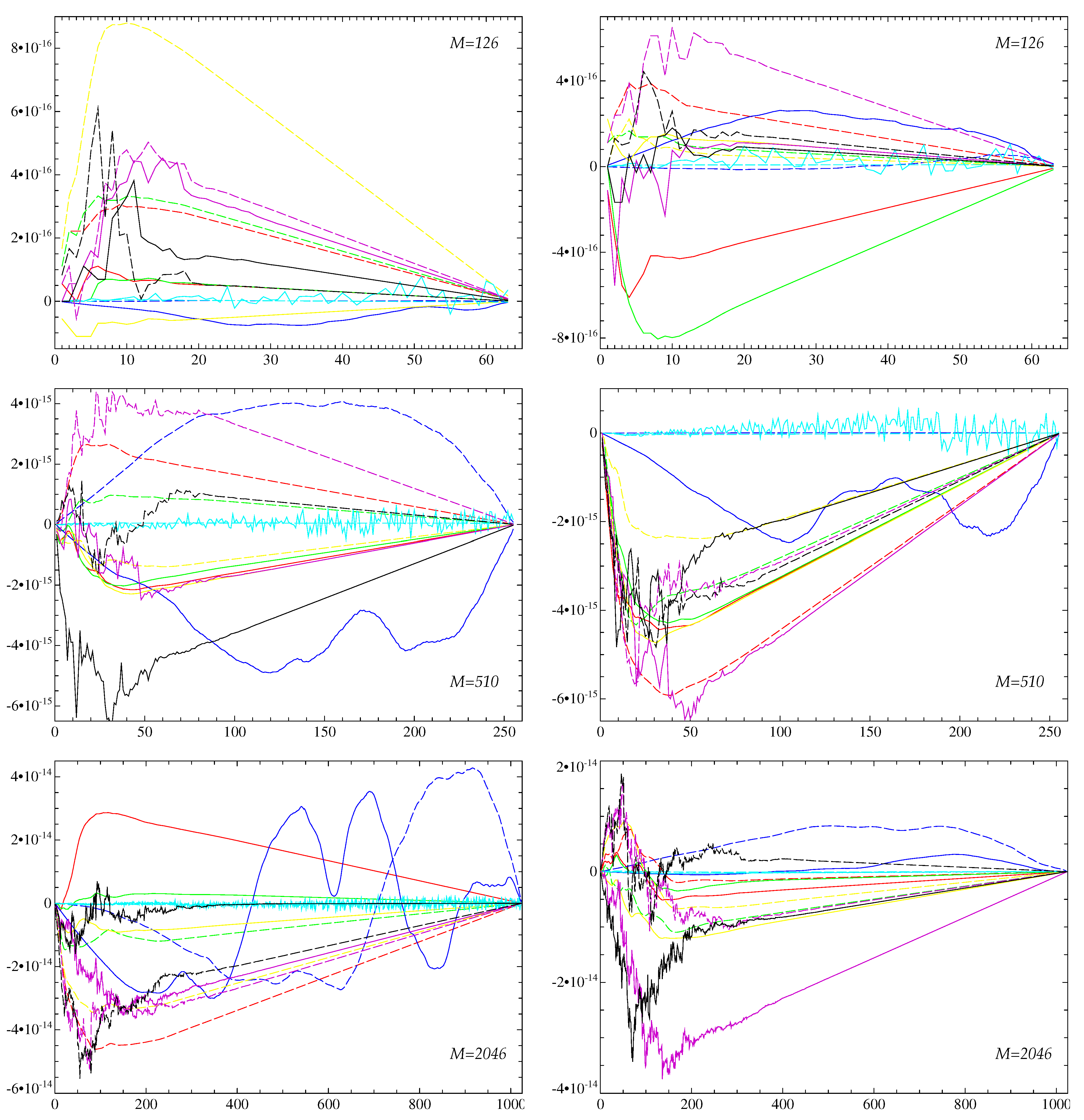
Figure 2 illustrates the error distributions among the approximate solutions ${\tilde{d}}_n$ to the sample test problems. Plots for two test problems for each of the three considered values of M are shown. The problem splits into two independent subproblems for odd- and even-number variables $d_k$; errors for odd-index coefficients are shown by continuous lines and for even-index coefficients by dashed lines. Graph colours indicate by which algorithms the curves have been obtained. We observe that algorithms 2 and 3 yield blatantly high errors; algorithms 2 and $2{}^{\prime }$ are also imperfect in that they produce higher errors for higher-index unknowns ${\tilde{d}}_n$. The errors experience a wild spiky behaviour for low-index coefficients $d_n$, but, except for algorithm $2{}^{\prime }$, it becomes more ordered roughly for $n>M/6$.

To assess how statistically relatively poor or good the considered algorithms are, we present in Figure 3 the distributions of error norms measured in the units of the smallest error norm for the given test problem. More precisely, the plots have been constructed by the following procedure: A set of ${10}^6$ test problems with solutions, pseudorandomly generated as discussed above, have been solved by each of the seven algorithms. For the pth problem and the kth algorithm, the error norms $\parallel {\mathbf{q}}^{(p;k)}\parallel$ have been determined. We denote the smallest of these seven norms by ${\omega }^{\left(p\right)}={min}_k\parallel {\mathbf{q}}^{(p;k)}\parallel$ and define the quantities $N_m^{\left(k\right)}$ as the number of cases (among the considered ${10}^6$ test problems), in which the error norm obtained by algorithm k relative to the smallest norm ${\omega }^{\left(p\right)}$ falls into the mth bin, or in other words, the ratio $\parallel {\mathbf{q}}^{(p;k)}\parallel /{\omega }^{\left(p\right)}$ satisfies the inequality $m-1<\parallel {\mathbf{q}}^{(p;k)}\parallel /{\omega }^{\left(p\right)}\le m$. In particular, $N_1^{\left(k\right)}$ is the number of test problems, for which algorithm k delivers the smallest, over all the seven algorithms, norm, i.e., ${\omega }^{\left(p\right)}=\parallel {\mathbf{q}}^{(p;k)}\parallel$. These computations have been performed for both norms, the maximum norm ${\parallel \mathbf{q}\parallel }_{max}$ and the energy norm ${\parallel \mathbf{q}\parallel }_{\mathrm{en}}$.

For each algorithm and both error norms, in Figure 3 we show the quantities $N_m^{\left(k\right)}$ versus the bin number m. The data points for six algorithms are joined into plots up to the smallest m such that $N_m^{\left(k\right)}=0$ (the use of the logarithmic scale for $N_m^{\left(k\right)}$ forces us to break the plot at this point). The outlier values $N_m^{\left(k\right)}>0$ for larger m are shown as disjoint points; all these values are small. The data distribution for algorithm 2 has a different nature, more resembling a cloud; we therefore render the data as two plots (for odd- and even-index numbers) only for the small-dimensional problem ($M=126$) for $N_m^{\left(3\right)}<100$. The outliers $N_m^{\left(k\right)}>0$ for $m>5\times {10}^3$ for $M=126$, and for $m>5\times {10}^4$ for $M=510$ and 2046 are ignored in Figure 3. There are 211 and 1529 such outliers for the odd- and even-index test problems, respectively, for algorithm 3 for $N=128$, 18 for the even-index problems for $M=510$, and 2265 and 8831 for the odd- and even-index test problems for $M=2046$. These statistics demonstrate that the larger the number of unknown coefficients M, the more the output of algorithm 2 is affected by the numerical noise.

The numerical results lead us to the following conclusions:

i.

Except for algorithm 2, in applications for solving the $3\times {10}^6$ test problems, for any M and for both error norms each algorithm delivers approximate solutions ${\tilde{d}}_n$ of any possible accuracy from the best to the worst one, i.e., for each algorithm, solutions to some test problems obtained by this algorithm have the smallest, the largest, or any differently placed intermediate error norm among the seven error norms obtained for this problem.

ii.

Algorithm 2 yields solutions of blantly poor accuracy. For $M=126$, its output still includes solutions occupying any possible place between the best-accuracy and worst-accuracy solutions. However, for $M=126$, it yields just three most accurate solutions in terms of the maximum error norm and just one, if the energy error norm is used. These numbers gradually increase via 46 and 15 penultimately worst-accuracy solutions to 999,934 and 999,975 least accurate solutions. By contrast, for $M=510$ and 2046 all its outputs are the least accurate solutions for both error norms, except for one case of penultimately worst-accuracy solutions for the maximum norm.

iii.

The error norms (see Table 1) are compatible with the standard “double” (in the Fortran speak; 64 bit words) computer precision (the ${10}^{-15}$ “machine epsilon”). The poor performance of algorithm 2 and the second-worst (accuracy-wise) algorithm 3 stems from the involvement in the expressions used in their formulation of the products of $d_1$ and $d_2$ with the numbers proportional to the indices of the unknown coefficients that increase up to the large numbers M.

iv.

We can regard the accuracy results at a different angle. In the worst-case scenario, the norm of a discrepancy in the r.h.s. of the equation $G\mathbf{d}=\mathbf{r}$ is multiplied by the condition number of the matrix G, which is defined as the product of norms of the matrices G and $G^{-1}$. The former norm is obviously order 1; to estimate the latter, we use (14) and (15) for the r.h.s. where all $r_k=1$, and find $\parallel G^{-1}{\parallel \ge \parallel \mathbf{d}\parallel }_{\mathrm{en}}/{\parallel \mathbf{r}\parallel }_{\mathrm{en}}=\mathrm{O}\left(M^2\right)$. Hence, the condition number of G is (at least) order $M^2$, which is compatible with the accuracy results for algorithm 2 (see maximum errors in Table 1). We observe that numerical errors are amplified by an algorithm-specific effective condition number [35], which can be much smaller than the worst-case theoretical condition number, provided a specialised algorithm takes into account particular properties of the problem,

v.

For all the three M values used, most frequently the smallest-error approximate solutions ${\tilde{d}}_n$ are provided by algorithm $2{}^{\prime }$ for whichever error norm: 315,174 and 236,707 times out of ${10}^6$ for $M=126$, 325,841 and 236,544 for $M=510$, and 333,062 and 239,009 for $M=2046$ (the first number in a pair is for the maximum error norm and the second one for the energy norm). Accuracy-wise, the shuttle algorithms 1 and $1{}^{\prime }$ are mutually close and not significantly inferior to algorithm $2{}^{\prime }$.

vi.

The quantities $N_m^{\left(k\right)}$ have the maxima at $k=2$ (see Figure 3), i.e., for each algorithm and each M, the error norms fall into the bin $1<\parallel {\mathbf{q}}^{(p;k)}\parallel /{\omega }^{\left(p\right)}\le 2$ with the highest probability.

vii.

Solutions ${\tilde{d}}_n$ obtained by all algorithms except for two and three have significantly larger errors $q_n$ for small n (say, for $n<M/6$) than for larger n (see Figure 3). By contrast, algorithms 2 and 3 yield maximum errors for intermediate and high n. In addition, the errors in solutions computed by algorithm 3 wildly oscillate, which is not typical for the behaviour of errors generated by the other six algorithms. Consequently, algorithms 2 and 3 yield approximate solutions in which ${\tilde{d}}_n$ for intermediate and high n have exceptionally high relative errors.

viii.

Algorithms 2 and $2{}^{\prime }$ are significantly faster than the other five algorithms (see Table 2). Their execution CPU times are mutually close and differ much more from the execution times registered for the other ones.

Properties iii and vii render algorithms 2 and 3 inapplicable. None of the seven algorithms is “perfect”, but the compromise between the highest efficiency and accuracy reveals the optimality of algorithm $2{}^{\prime }$.

3.2. Algorithms for Determining the Coefficients of a Linear Combination of $T_n^{★★}\left(x_3\right)$

The equation for the poloidal potential is obtained by applying twice the curl to (1a) and taking the vertical component of the result:

$$\begin{array}{cc}\hfill \frac{\partial {\nabla }_h^2{\nabla }^2{P}^{\mathbf{v}}}{\partial t}=& \mathrm{P}{\nabla }_h^2{\left({\nabla }^2\right)}^2{P}^{\mathbf{v}}+F^{p\mathbf{v}},\hfill \\ \hfill F^{p\mathbf{v}}=& -\sigma {\nabla }_h^2\theta +{\mathbf{e}}_3·(\tau (\mathbf{q}·\nabla )\nabla \times \mathbf{v}-{(\nabla \times )}^2(\mathbf{v}\times (\nabla \times \mathbf{v})-\mathbf{b}\times (\nabla \times \mathbf{b}))).\hfill \end{array}$$

The above equation is equivalent to the parabolic equation

$$\frac{\partial {\nabla }^2{P}^{\mathbf{v}}}{\partial t}=\mathrm{P}{\left({\nabla }^2\right)}^2{P}^{\mathbf{v}}+{\left({\nabla }_h^2\right)}^{-1}{F}^{p\mathbf{v}}.$$

(17)

To apply the inverse Laplacian ${\left({\nabla }^2\right)}^{-1}$ is now tempting but unfeasible, since the conditions (6b) do not imply suitable boundary conditions for ${\nabla }^2{P}^{\mathbf{v}}$. By (9), the polynomials

$$T_n^{★★}\left(x_3\right)=(n+1)(T_{n+4}\left(x_3\right)-T_{n+2}\left(x_3\right))-(n+3)(T_{n+2}\left(x_3\right)-T_n\left(x_3\right)),n\ge 0,$$

(18)

satisfy (6b), and the poloidal potentials can be approximated by finite series

$$P^{\mathbf{v}}(\mathbf{x},t)=\sum _{|n_1|\le N,|n_2|\le N,0\le n\le N-5}{p}_{\mathbf{n}}^{\mathbf{v}}\left(t\right){\mathrm{e}}^{\mathrm{i}({\alpha }_1{n}_1{x}_1+{\alpha }_2{n}_2{x}_2)}{T}_n^{★★}\left(x_3\right),$$

where $\mathbf{n}=(n_1,n_2,n)$.

Substituting the series into (17), we obtain an equation, whose l.h.s. is of the form

$$\sum _{|n_1|\le N,|n_2|\le N,0\le n\le N-1}\frac{\mathrm{d}{p}_{\mathbf{n}}^{\mathbf{v}}}{\mathrm{d}t}{\mathrm{e}}^{\mathrm{i}({\alpha }_1{n}_1{x}_1+{\alpha }_2{n}_2{x}_2)}{\tilde{p}}_n\left(x_3\right),$$

where ${\tilde{p}}_n$ is a polynomial of degree $n+4$. As usual, we apply the Fourier transform in the horizontal directions to deduce the equation for each pair of indices $n_1$ and $n_2$, and orthogonally project ${\tilde{p}}_n$ on the polynomials $T_m^{★★}\left(x_3\right)$ with the weight ${(1-x_3^2)}^{-1/2}$. Computing d$p_{\mathbf{n}}^{\mathbf{v}}/\mathrm{d}t$ requires inverting the matrices acting on the columnar vectors consisting of the time derivatives d$p_{\mathbf{n}}^{\mathbf{v}}/\mathrm{d}t$ for $0\le n\le N-1$ and $n_1,n_2$ fixed. As in the case of the toroidal potential of the flow, these are band matrices. To see this, we integrate twice by parts the integral ${\int }_{-1}^1{\mathrm{d}}^2{T}_n^{★★}/\mathrm{d}{x}_3^2{(1-x_3^2)}^{-1/2}{T}_m^{★★}\mathrm{d}{x}_3$ encountered in the projection of the l.h.s. of (17) (noting that the test polynomial $T_m^{★★}$ satisfies the boundary conditions (6b)) and apply the relation

$$\frac{{\mathrm{d}}^2}{\mathrm{d}{x}_3^2}\left({(1-x_3^2)}^{-1/2}{T}_m^{★★}\right)=4(m+1)(m+2)(m+3){(1-x_3^2)}^{-1/2}{T}_{m+2}.$$

(19)

It can be proven by using the identities

$$2(x_3^2-1)\frac{\mathrm{d}{T}_m}{\mathrm{d}{x}_3}=m(T_{m+1}-T_{m-1}),\frac{\mathrm{d}}{\mathrm{d}{x}_3}\left({(1-x_3^2)}^{1/2}\frac{\mathrm{d}{T}_m}{\mathrm{d}{x}_3}\right)=-m^2{(1-x_3^2)}^{-1/2}{T}_m.$$

Relation (19) is also useful for computing

$$\begin{array}{cc}\hfill {\int }_{-1}^1& {\left({\nabla }^2\right)}^2\left({\mathrm{e}}^{\mathrm{i}({\alpha }_1{n}_1{x}_1+{\alpha }_2{n}_2{x}_2)}{T}_n^{★★}\right){(1-x_3^2)}^{-1/2}{T}_m^{★★}\mathrm{d}{x}_3\hfill \\ \hfill & ={\mathrm{e}}^{\mathrm{i}({\alpha }_1{n}_1{x}_1+{\alpha }_2{n}_2{x}_2)}\left[\frac{\pi {\Gamma }^4}{2}\right((m+3)(m-3){\delta }_{n+4}^m-2\left((m+3)m+(m+2)(m-1)\right){\delta }_{n+2}^m\hfill \\ \hfill & +\left({(m+1)}^2+{(2m+4)}^2+{(m+3)}^2(1+{\delta }_0^m)\right){\delta }_n^m\hfill \\ \hfill & -2\left((m+1)(m+4)+(m+2)(m+5)\right){\delta }_{n-2}^m+(m+1)(m+7){\delta }_{n-4}^m)\hfill \\ \hfill & +4(m+1)(m+2)(m+3)(-\pi {\Gamma }^2\left((m-1){\delta }_{n+2}^m-2(m+2){\delta }_n^m+(m+5){\delta }_{n-2}^m\right)\hfill \\ \hfill & +{\int }_{-1}^1\frac{{\mathrm{d}}^2{T}_n^{★★}}{\mathrm{d}{x}_3^2}{(1-x_3^2)}^{-1/2}{T}_{m+2}\mathrm{d}{x}_3\left)\right],\hfill \end{array}$$

where $\Gamma ={({\alpha }_1^2{n}_1^2+{\alpha }_2^2{n}_2^2)}^{1/2}$ and ${\delta }_n^m$ is the Kronecker symbol. Differentiation in $x_3$ can now be performed ([9], see also [36]) using the recurrence relation

$$\frac{\mathrm{d}}{\mathrm{d}{x}_3}{T}_{k+1}=\frac{k+1}{k-1}\frac{\mathrm{d}}{\mathrm{d}{x}_3}{T}_{k-1}+2(k+1)T_k.$$

Thus, the vector $\mathbf{d}$ of the time derivatives of the expansion coefficients is a solution to the linear system of equations of the form

$$G\mathbf{d}=\mathbf{r},$$

(20a)

where $\mathbf{r}$ is the vector (of length $M^{\prime }=N-4$) of the dot products of the r.h.s. of (17) with $T_m^{★★}$; both G and $\mathbf{r}$ are divided by $\pi L_1{L}_2{\Gamma }^2/2$. The matrix has non-zero entries on the diagonal:

$$G_{k,k}=-6k^2-12k-8-9{\delta }_1^k-2{\Gamma }_k^{\prime }(k+1)$$

(20b)

and on four subdiagonals:

$$G_{k,k-4}=-(k-4)(k+2),G_{k,k-2}=4k^2-8+{\Gamma }_k^{\prime }(k-2),$$

(20c)

$$G_{k,k+2}=4{(k+2)}^2-8+{\Gamma }_k^{\prime }(k+4),G_{k,k+4}=-k(k+6),$$

(20d)

where

$${\Gamma }_k^{\prime }=4k(k+1)(k+2)/{\Gamma }^2.$$

(20e)

Algorithm 1 is the standard shuttle algorithm for a pentadiagonal matrix [37]. We note that the odd-index subproblem is separated from the even-index one and use the ansatz

$$d_n=A_n{d}_{n+2}+B_n{d}_{n+4}+C_n.$$

(21)

The first four equations imply

$$A_1=-G_{1,3}/G_{1,1},B_1=-G_{1,5}/G_{1,1},C_1=r_1/G_{1,1},$$

$$A_2=-G_{2,4}/G_{2,2},B_2=-G_{2,6}/G_{2,2},C_2=r_2/G_{2,2},$$

$$A_3=-\frac{B_1{G}_{3,1}+G_{3,5}}{A_1{G}_{3,1}+G_{3,3}},B_3=-\frac{G_{3,7}}{A_1{G}_{3,1}+G_{3,3}},C_3=\frac{r_3-G_{3,1}{C}_1}{A_1{G}_{3,1}+G_{3,3}},$$

$$A_4=-\frac{B_2{G}_{4,2}+G_{4,6}}{A_2{G}_{4,2}+G_{4,4}},B_4=-\frac{G_{4,8}}{A_2{G}_{4,2}+G_{4,4}},C_4=\frac{r_4-G_{4,2}{C}_2}{A_2{G}_{4,2}+G_{4,4}}.$$

The $M-4$ equations for $5\le n\le M$ yield the recurrence relations

$$A_n=-\frac{(G_{n,n-4}{A}_{n-4}+G_{n,n-2})B_{n-2}+G_{n,n+2}}{(G_{n,n-4}{A}_{n-4}+G_{n,n-2})A_{n-2}+G_{n,n-4}{B}_{n-4}+G_{n,n}},$$

$$B_n=-\frac{G_{n,n+4}}{(G_{n,n-4}{A}_{n-4}+G_{n,n-2})A_{n-2}+G_{n,n-4}{B}_{n-4}+G_{n,n}},$$

$$C_n=\frac{r_n-(G_{n,n-4}{A}_{n-4}+G_{n,n-2})C_{n-2}-G_{n,n-4}{C}_{n-4}}{(G_{n,n-4}{A}_{n-4}+G_{n,n-2})A_{n-2}+G_{n,n-4}{B}_{n-4}+G_{n,n}},$$

where it is assumed $G_{n,m}=0$ for $m>M$. This yields $d_n=C_n$ for $n=M-1$ and M, and we use the recurrence relation (21) to compute sequentially all the unknowns $d_n$ for decreasing n. (Note $B_n=0$ for $n=M-1$ and M.)

Algorithm 1${}^{\prime }$ is the same shuttle procedure applied to the system of equations with the reverse numbering of equations and variables.

Algorithms 2 and 2${}^{\prime }$ are modifications of the shuttle algorithm based on the observation that the sum of coefficients in the equation number k for $4<k<M-3$ is zero. Hence, in new variables $d_k^{\prime }=d_k-d_{k-2},k\ge 3$, the system reduces to a problem with a matrix $G^{\prime }$ involving three subdiagonals for $4<k<M-3$:

$$G_{k,k-2}^{\prime }={(k-1)}^2-9,G_{k,k}^{\prime }=-3k^2-2k-{\Gamma }_k^{\prime }(k-2),$$

$$G_{k,k+2}^{\prime }=3k^2+10k+8+{\Gamma }_k^{\prime }(k+4),G_{k,k+4}^{\prime }=-k(k+6).$$

The problem splits into two independent subproblems for odd- and even-number variables $d_k$. We formulate algorithm 2 for solving the subproblem for even-number variables; it is straightforward to reformulate it for the subproblem for odd-number variables. We introduce $M^{\prime }+1=M/2+1$ variables $z_1=d_2$, $z_k=d_{2k}-d_{2k-2}$ for $2\le k\le M^{\prime }$ and $z_{M^{\prime }+1}=d_{2M}$. They satisfy $M^{\prime }$ original equations and the gauge equation

$$z_{M^{\prime }+1}-\sum _{k=1}^{M^{\prime }}{z}_k=0.$$

(22)

The first equation is equivalent to $z_1=A_1{z}_2+B_1{z}_3+C_1$. Equations for $2\le k\le M^{\prime }$ take the form

$$G_{2k,2k-2}^{\prime }{z}_{k-1}+G_{2k,2k}^{\prime }{z}_k+G_{2k,2k+2}^{\prime }{z}_{k+1}+G_{2k,2k+4}^{\prime }{z}_{k+2}=r_{2k},$$

whereby

$$z_k=A_k{z}_{k+1}+B_k{z}_{k+2}+C_k,$$

(23)

$$A_k=-\frac{G_{2k,2k+2}^{\prime }+B_{k-1}{G}_{2k,2k-2}^{\prime }}{G_{2k,2k}^{\prime }+A_{k-1}{G}_{2k,2k-2}^{\prime }},B_k=\frac{-G_{2k,2k+4}^{\prime }}{G_{2k,2k}^{\prime }+A_{k-1}{G}_{2k,2k-2}^{\prime }},C_k=\frac{r_{2k}-C_{k-1}{G}_{2k,2k-2}^{\prime }}{G_{2k,2k}^{\prime }+A_{k-1}{G}_{2k,2k-2}^{\prime }},$$

which defines the first, “direct run of the shuttle”. Here, $z_{M^{\prime }+2}=0$. For $k=M^{\prime }$, the relation (23) reduces to just

$$z_k=D_k{z}_{M^{\prime }+1}+E_k,$$

(24)

where $D_{M^{\prime }}=A_{M^{\prime }}$ and $E_{M^{\prime }}=C_{M^{\prime }}$. We can now use (23) for $k=M^{\prime }-1,...,1$ to obtain the coefficients in (24) recursively,

$$D_k=A_k{D}_{k+1}+B_k{D}_{k+2},E_k=A_k{E}_{k+1}+B_k{E}_{k+2}+C_k$$

(the second, “reverse run of the shuttle”). Simultaneously, we compute the coefficients $F_k$ and $R_k$ in the partial sums

$$z_{M^{\prime }+1}-\sum _{n=k}^{M^{\prime }}{z}_n=F_k{z}_{M^{\prime }+1}+R_k.$$

By (22), we then find $z_{M^{\prime }+1}=-R_1/F_1$. Now, the third “run of the shuttle” yields

$$d_{2n}=\sum _{k=1}^n{z}_k=z_{M^{\prime }+1}-\sum _{k=n+1}^{M^{\prime }}{z}_k-\left(z_{M^{\prime }+1}-\sum _{k=1}^{M^{\prime }}{z}_k\right)=F_{n+1}{z}_{M^{\prime }+1}+R_{n+1}.$$

(25)

This algorithm is apparently more involved than the standard shuttle algorithm. However, since it works with the differences $z_k=d_{2k}-d_{2k-2}$, it may be advantageous in yielding more accurate values of $d_{2k}$.

Algorithm $2{}^{\prime }$ amounts to the same computational procedure applied to the system of equations, where the numbering of equations and variables is reversed. Thus, we obtain the relations, similar to (25), in which all $d_{2n}$ are expressed in terms of $z_1$ instead of $z_{M^{\prime }+1}$. Normally, the coefficients $d_k$ tend to zero, whereby $z_1$ is a priori much larger than $z_{M^{\prime }+1}$; for a given precision of computations (in our case, the standard real*8 “double” precision of the floating point arithmetics), this is a tighter constraint on the number of correct digits after the decimal point. Consequently, we may expect algorithm $2{}^{\prime }$ to yield less accurate values of $d_k$ than algorithm 2.

We have investigated the performance of the four algorithms following the same approach as for the algorithms for determining the coefficients of linear combinations of the polynomials $T_n^{★}$: we have synthesized ${10}^6$ pseudorandom sample test solutions $d_n$ by the same procedure, outlined in Section 3.1, as for the polynomials $T_n^{★}$, and analysed the errors $q_n={\tilde{d}}_n-d_n$ for the approximate solutions obtained by each of the four algorithms for $M=124$, 508 and 2044 terms in linear combinations of $T_n^{★★}$.

For each resolution parameter M and each algorithm,

Table 3. Minimum and maximum error norms detected among solutions to ${10}^6$ test problems (20a) by the four algorithms.

M	Algorithm	${\parallel \mathit{q}\parallel }_{max}$		${\parallel \mathit{q}\parallel }_{\mathbf{en}}$
		Min. Error	Max. Error	Min. Error	Max. Error
124	1	$4.51\times {10}^{-17}$	$3.22\times {10}^{-15}$	$1.10\times {10}^{-16}$	$8.47\times {10}^{-15}$
	$1{}^{\prime }$	$5.55\times {10}^{-17}$	$2.83\times {10}^{-15}$	$1.49\times {10}^{-16}$	$7.83\times {10}^{-15}$
	2	$5.55\times {10}^{-17}$	$3.55\times {10}^{-15}$	$1.42\times {10}^{-16}$	$1.02\times {10}^{-14}$
	$2{}^{\prime }$	$8.33\times {10}^{-17}$	$4.22\times {10}^{-15}$	$2.68\times {10}^{-16}$	$1.54\times {10}^{-14}$
508	1	$4.30\times {10}^{-16}$	$1.95\times {10}^{-14}$	$1.81\times {10}^{-15}$	$1.12\times {10}^{-13}$
	$1{}^{\prime }$	$2.78\times {10}^{-16}$	$2.03\times {10}^{-14}$	$1.98\times {10}^{-15}$	$1.10\times {10}^{-13}$
	2	$3.61\times {10}^{-16}$	$2.21\times {10}^{-14}$	$2.19\times {10}^{-15}$	$1.29\times {10}^{-13}$
	$2{}^{\prime }$	$5.00\times {10}^{-16}$	$2.07\times {10}^{-14}$	$2.47\times {10}^{-15}$	$1.27\times {10}^{-13}$
2044	1	$2.78\times {10}^{-15}$	$1.35\times {10}^{-13}$	$2.53\times {10}^{-14}$	$1.69\times {10}^{-12}$
	$1{}^{\prime }$	$2.53\times {10}^{-15}$	$1.33\times {10}^{-13}$	$2.95\times {10}^{-14}$	$1.62\times {10}^{-12}$
	2	$2.89\times {10}^{-15}$	$2.55\times {10}^{-13}$	$3.61\times {10}^{-14}$	$2.10\times {10}^{-12}$
	$2{}^{\prime }$	$3.16\times {10}^{-15}$	$1.53\times {10}^{-13}$	$3.32\times {10}^{-14}$	$1.88\times {10}^{-12}$

shows the ranges (i.e., the maximum and minimum values) of the maximum and energy norms of the approximate solution errors.

Table 4. Mean execution times (seconds) of 1000 applications of the four algorithms for computing coefficients of a linear combination of $T_n^{★★}$.

Algorithm	1	$1{}^{\prime }$	2	$2{}^{\prime }$
$M=124$	$1.41\times {10}^{-3}$	$1.51\times {10}^{-3}$	$1.43\times {10}^{-3}$	$1.51\times {10}^{-3}$
$M=508$	$6.04\times {10}^{-3}$	$6.30\times {10}^{-3}$	$5.88\times {10}^{-3}$	$6.18\times {10}^{-3}$
$M=2044$	$2.506\times {10}^{-2}$	$2.632\times {10}^{-2}$	$2.464\times {10}^{-2}$	$2.595\times {10}^{-2}$

illustrates the execution times for each algorithm, measured by the same procedure (see Section 3.1) as for the polynomials $T_n^{★}$. The obtained mean execution times are again accurate to at least three significant digits. We expect the algorithm 1 execution times to coincide with those for algorithm $1{}^{\prime }$, similarly for algorithms 2 and $2{}^{\prime }$. However, the times presented in Table 4 for algorithms 1 and 2 are slightly smaller than those for algorithms $1{}^{\prime }$ and $2{}^{\prime }$, respectively. This difference is insignificant, it just reflects the way we have programmed the latter algorithms: in our implementation, the orders of the equations and unknown variables are reversed at run time, which can be avoided by a more careful programming of the algorithms using index reversion.

Figure 4 illustrates the error distributions among the unknowns detected for solutions to six sample test problems (plots for two problems for all the considered $M=124$, 508 and 2044 are shown). Figure 5 presents the distributions of error norms measured by the same procedure, discussed in Section 3.1, as for the polynomials $T_n^{★}$. For the pth problem and the kth algorithm, we find the error norms $\parallel {\mathbf{q}}^{(p;k)}\parallel$ and the smallest norm for this problem, ${\omega }^{\left(p\right)}={min}_k\parallel {\mathbf{q}}^{(p;k)}\parallel$. We again denote by $N_m^{\left(k\right)}$ the number of cases, among the ${10}^6$ test problems, in which the error norm produced by algorithm k, measured in the units of ${\omega }^{\left(p\right)}$, falls into the mth bin, i.e., m satisfies the inequality $m-1<\parallel {\mathbf{q}}^{(p;k)}\parallel /{\omega }^{\left(p\right)}\le m$. For each algorithm and both error norms (the maximum norm and the energy norm), Figure 5 shows the histogram $N_m^{\left(k\right)}$ versus the bin number m. The data points are joined up to the smallest m such that $N_m^{\left(k\right)}=0$, and the outlier values $N_m^{\left(k\right)}>0$ (always small) for larger m are shown as disjoint points; unlike in Figure 3, all outliers are shown.

The results reveal the following properties of the algorithms:

i.

None of the four algorithms is “perfect”: for all considered M and for both error norms, when solving the $3\times {10}^6$ test problems each algorithm delivers solutions of any possible relative accuracy from the best to the worst one, in the sense that solutions to some test problems obtained by any algorithm have the smallest, the largest or any intermediate error norms among the four error norms produced by the four algorithms for this problem.

ii.

The quantities $N_m^{\left(k\right)}$ have the maxima at $m=2$ (see Figure 5), i.e., for each algorithm the error norms fall into the second bin, $1<\parallel {\mathbf{q}}^{(p;k)}\parallel /{\omega }^{\left(p\right)}\le 2$, with the highest probability.

iii.

For any M and for both error norms, algorithm $1{}^{\prime }$ delivers the best accuracy solutions (has the maximum $N_1^{\left(k\right)}$ over k) more often than the other three. For $M=124$ and 508, the least accurate solutions are obtained most frequently by algorithm $2{}^{\prime }$ and for $M=2044$ by algorithm 2.

iv.

The errors $q_n$ for intermediate and high n (say, for $n>M/6$) in approximate solutions computed by algorithm $2{}^{\prime }$ are significantly larger than in solutions obtained by any of the other three algorithms.

v.

The execution CPU times of algorithms 1 and $1{}^{\prime }$ are slightly larger than those for algorithms 2 and $2{}^{\prime }$.

Property iv implies that algorithm $2{}^{\prime }$ yields approximate solutions, where ${\tilde{d}}_n$ for intermediate and high n are polluted by high relative errors, rendering this algorithm inapplicable. The smallest execution time and the highest frequency of yielding the smallest errors distinguish algorithm $1{}^{\prime }$, but algorithms 2 and $2{}^{\prime }$ follow closely.

4. Discretisation of the Magnetic Field

Here we consider the implications of the boundary conditions (2b) for the magnetic field. Since the magnetic field is solenoidal (1d), it can be decomposed into the sum of the toroidal, ${\mathbf{T}}^{\mathbf{b}}(\mathbf{x},t)$, poloidal, ${\mathbf{P}}^{\mathbf{b}}(\mathbf{x},t)$, and mean-field, ${\mathbf{M}}^{\mathbf{b}}(\mathbf{x},t)$, components:

$$\begin{array}{cc}\hfill \mathbf{b}(\mathbf{x},t)=& {\mathbf{T}}^{\mathbf{b}}(\mathbf{x},t)+{\mathbf{P}}^{\mathbf{b}}(\mathbf{x},t)+{\mathbf{M}}^{\mathbf{b}}(x_3,t),\hfill \end{array}$$

(26a)

$$\begin{array}{cc}\hfill {\mathbf{T}}^{\mathbf{b}}(\mathbf{x},t)=& \nabla \times \left(T^{\mathbf{b}}(\mathbf{x},t){\mathbf{e}}_3\right),\hfill \end{array}$$

(26b)

$$\begin{array}{cc}\hfill {\mathbf{P}}^{\mathbf{b}}(\mathbf{x},t)=& \nabla \times \nabla \times \left(P^{\mathbf{b}}(\mathbf{x},t){\mathbf{e}}_3\right),\hfill \end{array}$$

(26c)

$$\begin{array}{cc}\hfill {\mathbf{M}}^{\mathbf{b}}(x_3,t)=& {\langle (b^1(\mathbf{x},t),b^2(\mathbf{x},t),0)\rangle }_h\hfill \end{array}$$

(26d)

such that

$${〈T^{\mathbf{b}}〉}_h={〈P^{\mathbf{b}}〉}_h=0.$$

In view of the boundary conditions (2b) and (2c) for the magnetic field, the potentials and the mean-field component satisfy the boundary conditions

$${T^b|}_{x_3=1}={\frac{\partial T^b}{\partial x_3}|}_{x_3=-1}=0,$$

(27a)

$${\nabla P^b|}_{x_3=1}={\nabla h|}_{x_3=1^{\prime }}$$

(27b)

$${\frac{{\partial }^2{P}^b}{\partial x_3^2}|}_{x_3=-1}={P^b|}_{x_3=-1}=0,$$

(27c)

$${M^b|}_{x_3=1}={\frac{\partial M^b}{\partial x_3}|}_{x_3=-1}=0.$$

(27d)

The poloidal potential is determined from the vertical component of (1b), the toroidal one from the vertical component of the curl of (1b),

$$\frac{\partial T^{\mathbf{b}}}{\partial t}=\eta {\nabla }^2{T}^{\mathbf{b}}+{\left({\nabla }_h^2\right)}^{-1}{F}^{t\mathbf{b}},F^{t\mathbf{b}}={\mathbf{e}}_3·{(\nabla \times )}^2(\mathbf{v}\times \mathbf{b}),$$

(28)

and the mean-field component of the magnetic field from the equation derived by averaging over horizontal variables of the horizontal component of (1b).

The harmonic function h referred to in (27a) is defined by (2b). The boundary condition (27b) can be further detailed for individual harmonics in horizontal variables for the poloidal potential expanded as the Fourier series

$$\begin{array}{cc}\hfill P^{\mathbf{b}}(\mathbf{x},t)=& \sum _{|n_1|\le N,|n_2|\le N}{P}_{n_1,n_2}^{\mathbf{b}}(x_3,t){\mathrm{e}}^{\mathrm{i}({\alpha }_1{n}_1{x}_1+{\alpha }_2{n}_2{x}_2)}\hfill \\ \hfill \Rightarrow \nabla P^{\mathbf{b}}=& \sum _{|n_1|\le N,|n_2|\le N}\left(\mathrm{i}{\alpha }_1{n}_1{P}_{n_1,n_2}^{\mathbf{b}},\mathrm{i}{\alpha }_2{n}_2{P}_{n_1,n_2}^{\mathbf{b}},\frac{\partial P_{n_1,n_2}^{\mathbf{b}}}{\partial x_3}\right){\mathrm{e}}^{\mathrm{i}({\alpha }_1{n}_1{x}_1+{\alpha }_2{n}_2{x}_2)}.\hfill \end{array}$$

At the upper boundary $x_3=1$, the horizontal components of the gradient of $P_{n_1,n_2}^{\mathbf{b}}$ coincide with the gradient of the harmonic function

$$h(\mathbf{x},t)=P_{n_1,n_2}^{\mathbf{b}}(1,t){\mathrm{e}}^{\mathrm{i}({\alpha }_1{n}_1{x}_1+{\alpha }_2{n}_2{x}_2)-{({\alpha }_1^2{n}_1^2+{\alpha }_2^2{n}_2^2)}^{1/2}(x_3-1)}$$

and therefore (27b) is satisfied as long as

$$\frac{\partial P_{n_1,n_2}^{\mathbf{b}}}{\partial x_3}{\left.\phantom{{|}_{|}}\right|}_{x_3=1}=-{({\alpha }_1^2{n}_1^2+{\alpha }_2^2{n}_2^2)}^{1/2}{\left.P_{n_1,n_2}^{\mathbf{b}}\phantom{{|}_{|}}\right|}_{x_3=1}.$$

(29)

In view of (9), the boundary condition (27c) is satisfied by the polynomials

$${\mathrm{\Pi }}_n=(n+1)(2n+1)T_{n-1}+(4n^2+2)T_n+(n-1)(2n-1)T_{n+1}forn\ge 0$$

and both conditions, (27c) and (29), are satisfied by the polynomials

$$\begin{gathered} T_n^{★★★}\left(x_3\right)=((4{\left(n+1\right)}^4-2{\left(n+1\right)}^2+1+\mathsf{\Gamma }(4{\left(n+1\right)}^2+2)){\mathsf{\Pi }}_n \\ -\left(4n^4-2n^2+1+\mathsf{\Gamma }(4n^2+2)){\mathsf{\Pi }}_{n+1}\right)/\left(2n+1\right) \\ ={\mathsf{\kappa }}_{n+1}{T}_{n-1}+\left({\mathsf{\kappa }}_n+{\mathsf{\lambda }}_n\right)T_n-\left({\mathsf{\kappa }}_{n+1}-{\mathsf{\lambda }}_n\right)T_{n+1}-{\mathsf{\kappa }}_n{T}_{n+2} \end{gathered}$$

(30)

for $n\ge 1$, where

$${\mathsf{\kappa }}_n=n\left(4n^4-2n^2+1+\mathsf{\Gamma }\left(4n^2+2\right)\right),{\mathsf{\lambda }}_n=16n\left(n+1\right)\left(n\left(n+1\right)+1\right).$$

Thus, $P_{n_1, n_2}^b\left(x_3,t\right)$can be expanded as

$$P^{\mathbf{b}}(\mathbf{x},t)=\sum _{|n_1|\le N,|n_2|\le N,1\le n\le N-2}{p}_{\mathbf{n}}^{\mathbf{b}}\left(t\right){\mathrm{e}}^{\mathrm{i}({\alpha }_1{n}_1{x}_1+{\alpha }_2{n}_2{x}_2)}{T}_n^{★★★}\left(x_3\right).$$

The vector $\mathbf{d}$ of the time derivatives of the coefficients of the expansion is a solution to the linear system of equations of the form $G\mathbf{d}=\mathbf{r}$. Here G is the heptadiagonal Gram matrix for the basic functions $T_m^{★★★}$ and $\mathbf{r}$ is the vector (of length $M^{″}=N-3$) of dot products of the r.h.s. with $T_m^{★★★}$. Unlike in the two linear problems considered above, there is no separation into odd- and even-index subproblems.

The shuttle process can again be applied for solving this problem. We use the ansatz

$$d_n=A_n{d}_{n+1}+B_n{d}_{n+2}+C_n{d}_{n+3}+D_n.$$

(31)

The first equation is equivalent to

$$A_1=-G_{1,2}/G_{1,1},B_1=-G_{1,3}/G_{1,1},C_1=-G_{1,4}/G_{1,1},D_1=r_1/G_{1,1}.$$

The second equation implies

$$A_2=-(G_{2,1}{B}_1+G_{2,3})/A_2^{\prime },B_2=-(G_{2,1}{C}_1+G_{2,4})/A_2^{\prime },$$

$$C_2=-G_{2,5}/A_2^{\prime },D_2=(r_2-G_{2,1}{D}_1)/A_2^{\prime },$$

where

$$A_2^{\prime }=G_{2,1}{A}_1+G_{2,2}.$$

From the third equation,

$$A_3=-(A_3^{\prime }{B}_2+G_{3,1}{C}_1+G_{3,4})/A_3^{″},B_3=-(A_3^{\prime }{C}_2+G_{3,5})/A_3^{″},C_3=-G_{3,6}/A_3^{″},$$

$$D_3=(r_3-G_{3,1}{D}_1-A_3^{\prime }{D}_2)/A_3^{″},$$

where

$$A_3^{\prime }=G_{3,1}{A}_1+G_{3,2},A_3^{″}=A_3^{\prime }{A}_2+G_{3,1}{B}_1+G_{3,3}.$$

For $n\ge 4$, it is convenient to introduce the additional variables

$$A_n^{\prime }=G_{n,n-3}{A}_{n-3}+G_{n,n-2},A_n^{″}=A_n^{\prime }{A}_{n-2}+G_{n,n-3}{B}_{n-3}+G_{n,n-1},$$

$$A_n^{‴}=A_n^{″}{A}_{n-1}+A_n^{\prime }{B}_{n-2}+G_{n,n-3}{C}_{n-3}+G_{n,n}.$$

For $4\le n\le M^{″}-3$, in the nth equation we use (21) to make consecutive substitutions of $d_{n-2},d_{n-1}$ and $d_n$. This yields the recurrence relations

$$A_n=-(A_n^{″}{B}_{n-1}+A_n^{\prime }{C}_{n-2}+G_{n,n+1})/A_n^{‴},B_n=-(A_n^{″}{C}_{n-1}+G_{n,n+2})/A_n^{‴},$$

$$C_n=-G_{n,n+3}/A_n^{‴},D_n=(r_n-G_{n,n-3}{D}_{n-3}-A_n^{\prime }{D}_{n-2}-A_n^{″}{D}_{n-1})/A_n^{‴}.$$

Finally, the remaining equations for $M^{″}-2\le n\le M^{″}$ yield a system of three equations in $d_{M^{″}-2},d_{M^{″}-1}$ and $d_{M^{″}}$. The equations are:

$$(A_n^{″}{A}_{n-1}+A_n^{\prime }{B}_{n-2}+G_{n,n-3}{C}_{n-3}+G_{n,n})d_{M^{″}-2}+(A_n^{″}{B}_{n-1}+A_n^{\prime }{C}_{n-2}+G_{n,n+1})d_{M^{″}-1}$$

$$+(A_n^{″}{C}_{n-1}+G_{n,n+2})d_{M^{″}}=r_{M^{″}-2}-A_n^{″}{D}_{n-1}-A_n^{\prime }{D}_{n-2}-G_{n,n-3}{D}_{n-3}$$

for $n=M^{″}-2$;

$$(A_n^{\prime }{A}_{n-2}+G_{n,n-3}{B}_{n-3}+G_{n,n-1})d_{M^{″}-2}+(A_n^{\prime }{B}_{n-2}+G_{n,n-3}{C}_{n-3}+G_{n,n})d_{M^{″}-1}+$$

$$(A_n^{\prime }{C}_{n-2}+G_{n,n+1})d_{M^{″}}=r_{M^{″}-1}-A_n^{\prime }{D}_{n-2}-G_{n,n-3}{D}_{n-3}$$

for $n=M^{″}-1$;

$$(G_{n,n-3}{A}_{n-3}+G_{n,n-2})d_{M^{″}-2}+(G_{n,n-3}{B}_{n-3}+G_{n,n-1})d_{M^{″}-1}+$$

$$(G_{n,n-3}{C}_{n-3}+G_{n,n})d_{M^{″}}=r_{M^{″}}-G_{n,n-3}{D}_{n-3}$$

for $n=M^{″}$.

The boundary conditions (27a) and (27d) for the toroidal potential and mean-field components of the magnetic field are satisfied by the polynomials

$$T_n^{★★★★}\left(x_3\right)={\mathsf{\mu }}_n{T}_{n-1}-4n{T}_n-{\mathsf{\mu }}_{n-1}{T}_{n+1},\mathrm{where}{\mathsf{\mu }}_n=2n\left(n+1\right)+1,$$

(32)

and hence we use the expansions

$$T^b\left(x,t\right)={\displaystyle \sum }_{\left|n_1\right|\le N,\left|n_2\right|\le N,1\le n\le N-2}{t}_n^b\left(t\right){\mathrm{e}}^{\mathrm{i}\left({\mathsf{\alpha }}_1{n}_1{x}_1+{\mathsf{\alpha }}_2{n}_2{x}_2\right)}{T}_n^{★★★★}\left(x_3\right),$$

$$M^b\left(x_3,t\right)={\displaystyle \sum }_{0\le n\le N}{M}_n^b\left(t\right)T_n^{★★★★}\left(x_3\right).$$

The coefficients in the expansion of a function in this basis can be determined by solving a linear system of equations with a pentadiagonal Gram matrix G, whose non-zero entries are as follows:

$$G_{k,k-2}=-{\mathsf{\mu }}_{k-3}{\mathsf{\mu }}_k,G_{k,k-1}=-4\left(k-1\right){\mathsf{\mu }}_k+4k{\mathsf{\mu }}_{k-2},G_{k,k}={\mathsf{\mu }}_k^2\left(1+{\mathsf{\delta }}_1^k\right)+16k^2+{\mathsf{\mu }}_{k-1}^2,$$

$$G_{k,k+1}=-4k{\mathsf{\mu }}_{k+1}+4\left(k+1\right){\mathsf{\mu }}_{k-1},G_{k,k+2}=-{\mathsf{\mu }}_{k-1}{\mathsf{\mu }}_{k+2}.$$

Apparently, the system has no special properties enabling us to develop specialized methods for solving it numerically; it can be solved by the shuttle method (see Algorithm 1 in Section 3.2).

5. Conclusions

We have presented an original algorithm for numerical solution of the equations of convective dynamo in a plane horizontal layer rotating about an inclined axis under geophysically sound boundary conditions. In many respects, our approach does not differ significantly from the general approach that was followed by other authors. Focusing mainly on the accuracy of computations, especially in the small scales, we have discussed the numerical techniques which we have designed with this purpose in mind.

The Galerkin method is applied for computing the toroidal and poloidal components of physical vector fields and their mean components. We exploit the bases of functions that are products of linear combinations ($T_n^{★}\left(10\right)$, $T_n^{★★}\left(18\right)$, $T_n^{★★★}\left(30\right)$, and $T_n^{★★★★}\left(32\right)$) of Chebyshev polynomials in the vertical coordinate and Fourier harmonics in the horizontal coordinates. The basic functions involving the polynomials $T_n^{★}$ are used for the spatial discretisation of the unknown functions that take zero values on the horizontal boundaries $x_3=\pm 1$, namely, in the problem under discussion, the toroidal potential ofthe flow and its mean fields, and the deviation of temperature from the steady-state linear profile. The poloidal potential of the flow, which, for the no-slip boundary conditions, must vanish on the horizontal boundaries together with the first derivative in the vertical direction, is expanded in a series of functions involving the polynomial factors $T_n^{★★}$. The functions involving $T_n^{★★★}$ are used for discretising the poloidal potential of the magnetic field in the presence of the dielectric over the fluid layer and an electric conductor below it; while the no-slip boundary conditions for a solenoidal field are often considered in different problems, the latter boundary conditions are rather special. Finally, the toroidal potential of the magnetic field, which, for the boundary conditions considered here, is zero on the upper fluid boundary, and whose first derivative in $x_3$ vanishes on the lower boundary, is expanded in the series of the basic functions involving the polynomials $T_n^{★★★★}$.

The basic functions satisfy the boundary conditions, but they are non-orthogonal. Specialized algorithms for determining the coefficients in the expansion of an arbitrary function in a series of the basic functions involving polynomials $T_n^{★}$ and $T_n^{★★}$ are proposed and analyzed.. They are general-purpose and are applicable whenever the same boundary conditions are imposed. We find that when the spatial resolution is sufficiently high, our original algorithm $2{}^{\prime }$ is optimal from the point of view of accuracy and efficiency when $T_n^{★}$ are used, and algorithm $1{}^{\prime }$ (the reverse shuttle algorithm) is optimal for $T_n^{★★}$.

References

1. Podvigina, O.M. A route to magnetic field reversals: An example of an ABC-forced non-linear dynamo. Geophys. Astrophys. Fluid Dyn. 2003, 97, 149–174. [Google Scholar] [CrossRef]
2. Chertovskih, R.; Gama, S.M.A.; Podvigina, O.; Zheligovsky, V. Dependence of magnetic field generation by thermal convection on the rotation rate: A case study. Physica D 2010, 239, 1188–1209. [Google Scholar] [CrossRef]
3. Jones, C.A.; Roberts, P.H. Convection-driven dynamos in a rotating plane layer. J. Fluid Mech. 2000, 404, 311–343. [Google Scholar] [CrossRef]
4. Rotvig, J.; Jones, C.A. Rotating convection-driven dynamos at low Ekman number. Phys. Rev. E 2002, 66, 056308. [Google Scholar] [CrossRef]
5. Eltayeb, I.A.; Rahman, M.M. Model III: Benard convection in the presence of horizontal magnetic field and rotation. Phys. Earth Planet. Inter. 2013, 221, 38–59. [Google Scholar] [CrossRef]
6. Zheligovsky, V. Space analyticity and bounds for derivatives of solutions to the evolutionary equations of diffusive magnetohydrodynamics. Mathematics 2021, 9, 1789. [Google Scholar] [CrossRef]
7. Stellmach, S.; Hansen, U. An efficient spectral method for the simulation of dynamos in Cartesian geometry and its implementation on massively parallel computers. Geochem. Geophys. Geosyst. 2008, 9, Q05003. [Google Scholar] [CrossRef]
8. Fox, L.; Parker, I.B. Chebyshev Polynomials in Numerical Analysis; Oxford University Press: London, UK, 1968. [Google Scholar]
9. Canuto, C.; Hussaini, M.Y.; Quarteroni, A.; Zang, T.A. Spectral Methods in Fluid Dynamics; Springer: Berlin/Heidelberg, Germany, 1988. [Google Scholar] [CrossRef]
10. Peyret, R. Spectral Methods for Incompressible Viscous Flow; Springer: Berlin/Heidelberg, Germany, 2002. [Google Scholar] [CrossRef]
11. Kleiser, L.; Schumann, U. Treatment of incompressibility and boundary conditions in 3-D numerical spectral simulations of plane channel flows. In Proceedings of the Third GAMM—Conference on Numerical Methods in Fluid Mechanics, Cologne, Germany, 10–12 October 1979; Hirschel, E.H., Ed.; Notes on Numerical Fluid Mechanics; Vieweg+Teubner Verlag: Wiesbaden, Germany, 1980; Volume 2, pp. 165–173. [Google Scholar]
12. Werne, J. Incompressibility and no-slip boundaries in the Chebyshev-Tau approximation: Correction to Kleiser and Schumann’s influence-matrix solution. J. Comput. Phys. 1995, 120, 260–265. [Google Scholar] [CrossRef]
13. Meseguer, Á.; Trefethen, L.N. Linearized pipe flow to Reynolds number 107. J. Comput. Phys. 2003, 186, 178–197. [Google Scholar] [CrossRef]
14. O’Connor, L.; Lecoanet, D.; Anders, E.H. Marginally stable thermal equilibria of Rayleigh–Bénard convection. Phys. Rev. Fluids 2021, 6, 093501. [Google Scholar] [CrossRef]
15. Reetz, F.; Schneider, T. Invariant states in inclined layer convection. Part 1. Temporal transitions along dynamical connections between invariant states. J. Fluid Mech. 2020, 898, A22. [Google Scholar] [CrossRef]
16. Wen, B.; Goluskin, D.; LeDuc, M.; Chini, G.P.; Doering, C.R. Steady Rayleigh–Bénard convection between stress-free boundaries. J. Fluid Mech. 2020, 905, R4. [Google Scholar] [CrossRef]
17. Wen, B.; Goluskin, D.; Doering, C.R. Steady Rayleigh–Bénard convection between no-slip boundaries. J. Fluid Mech. 2022, 933, R4. [Google Scholar] [CrossRef]
18. Alboussière, T.; Drif, K.; Plunian, F. Dynamo action in sliding plates of anisotropic electrical conductivity. Phys. Rev. E 2020, 101, 033107. [Google Scholar] [CrossRef]
19. Sreenivasan, B.; Gopinath, V. Confinement of rotating convection by a laterally varying magnetic field. J. Fluid Mech. 2017, 822, 590–616. [Google Scholar] [CrossRef]
20. Perez-Espejel, D.; Avila, R. Linear stability analysis of the natural convection in inclined rotating parallel plates. Phys. Lett. A 2019, 383, 859–866. [Google Scholar] [CrossRef]
21. Gottlieb, D.; Orszag, S.A. Numerical Analysis of Spectral Methods: Theory and Applications; SIAM-CBMS: Philadelphia, USA, 1977. [Google Scholar]
22. Tuckerman, L.S. Divergence-free velocity fields in nonperiodic geometries. J. Comput. Phys. 1989, 80, 403–441. [Google Scholar] [CrossRef]
23. Cox, S.M.; Matthews, P.C. Exponential time differencing for stiff systems. J. Comput. Phys. 2002, 176, 430–455. [Google Scholar] [CrossRef]
24. Chertovskih, R.; Rempel, E.L.; Chimanski, E.V. Magnetic field generation by intermittent convection. Phys. Lett. A 2017, 381, 3300–3306. [Google Scholar] [CrossRef]
25. Chertovskih, R.; Chimanski, E.V.; Rempel, E.L. Route to hyperchaos in Rayleigh–Bénard convection. Europhys. Lett. 2015, 112, 14001. [Google Scholar] [CrossRef]
26. Jeyabalan, S.R.; Chertovskih, R.; Gama, S.; Zheligovsky, V. Nonlinear large-scale perturbations of steady thermal convective dynamo regimes in a plane layer of electrically conducting fluid rotating about the vertical axis. Mathematics 2022, 10, 2957. [Google Scholar] [CrossRef]
27. Braginsky, S.I.; Roberts, P.H. Equations governing convection in Earth’s core and the geodynamo. Geophys. Astrophys. Fluid Dynamics 1995, 79, 1–97. [Google Scholar] [CrossRef]
28. Boyd, J.P. Chebyshev and Fourier Spectral Methods; Dover: Downers Grove, IL, USA, 2001. [Google Scholar]
29. Schmitt, B.J.; von Wahl, W. Decomposition of solenoidal fields into poloidal fields, toroidal fields and the mean flow. Applications to the Boussinesq–equations. In The Navier–Stokes Equations II—Theory and Numerical Methods. Proceedings, Oberwolfach 1991; Lecture Notes in Math; Heywood, J.G., Masuda, K., Rautmann, R., Solonnikov, S.A., Eds.; Springer: Berlin, Germany, 1992; Volume 1530, pp. 291–305. [Google Scholar] [CrossRef]
30. Lanczos, C. Applied Analysis; Prentice-Hall: Englewood Cliffs, NJ, USA, 1956. [Google Scholar]
31. Madabhushi, R.K.; Balachandar, S.; Vanka, S.P. A divergence-free Chebyshev collocation procedure for incompressible flows with two non-periodic directions. J. Comput. Phys. 1993, 105, 199–206. [Google Scholar] [CrossRef]
32. Rivlin, T.J. Chebyshev Polynomials: From Approximation Theory to Algebra and Number Theory; Wiley-Interscience: Hoboken, NJ, USA, 1974. [Google Scholar]
33. Shen, J. Efficient spectral-Galerkin method II. Direct solvers of second and fourth order equations by using Chebyshev polynomials. SIAM J. Sci. Comput. 1995, 16, 74–87. [Google Scholar] [CrossRef]
34. Godunov, S.K.; Ryabenkii, V.S. Difference Schemes. An Introduction to the Underlying Theory, 1st ed.; Elsevier: Amsterdam, The Netherlands, 1987. [Google Scholar]
35. Li, Z.-C.; Chien, C.-S.; Huang, H.-T. Effective condition number for finite difference method. J. Comp. Appl. Math. 2007, 198, 208–235. [Google Scholar] [CrossRef]
36. Mason, J.C.; Handscomb, D.C. Chebyshev Polynomials; CRC Press: Boca Raton, FL, USA, 2003. [Google Scholar] [CrossRef]
37. Il’in, V.P.; Karpov, V.V.; Maslennikov, A.M. Numerical Methods for Solving Structural Mechanics Problems. A Handbook; Vyshaishaya Shkola: Minsk, Russia, 1990. [Google Scholar]
Figure 1. An illustrative sketch of the physical process: there is a dielectric over the upper horizontal boundary (blue) of the fluid layer (white), the lower horizontal boundary (gray) is electrically conducting, and the flow satisfies the no-slip boundary conditions at the boundaries. The fluid layer is rotating about the axis, whose arbitrary direction is shown by the unit vector q (magenta), the Cartesian coordinate system (orange colour, respectively) is co-rotating with the fluid.
Mathematics 11 00808 g001
Figure 2. Errors (vertical axes) of approximate solutions obtained for sample test problems by algorithms 1 (red), 1 (green), 2 (blue), 2 (yellow), 3 (cyan), 3 (magenta) and 4 (black colour, respectively) for determining the coefficients of a linear combination of T n ( x 3 ) vs. the coefficient index number (horizontal axes). The panels show the plots for six randomly chosen sample runs for the three values of the resolution parameter M. Continuous line: odd-index coefficients; dashed line: even-index coefficients. In order to fit the panels, the error values have been divided by 10 3 for algorithm 2 and by 10 2 for algorithm 3.
Mathematics 11 00808 g002
Figure 3. Distribution of error norms of approximate solutions obtained for 10 6 test problems by algorithms 1 (red), 1 (green), 2 (blue), 2 (yellow), 3 (cyan), 3 (magenta) and 4 (black colour, respectively) for determining the coefficients of a linear combination of T n ( x 3 ) . Horizontal axis: the error norms relative to the smallest error norm obtained for the test problem by the seven algorithms, m; vertical axis: the number of cases, N m ( k ) , for the kth algorithm and each error norm. Dashed lines, saturated colours: the maximum error norm; continuous lines, diluted colours: the energy error norm. The panels show the plots for the three values of the resolution parameter M.
Mathematics 11 00808 g003
Figure 4. Errors (vertical axes) of approximate solutions obtained for sample test problems by algorithms 1 (red), 1 (green), 2 (blue) and 2 (black colour, respectively) for determining the coefficients of a linear combination of T n ( x 3 ) vs. the coefficient index number (horizontal axes). The panels show the plots for six randomly chosen sample runs for the three values of the resolution parameter M. Continuous line: odd-index coefficients; dashed line: even-index coefficients.
Mathematics 11 00808 g004
Figure 5. Distribution of error norms of approximate solutions obtained for 10 6 sample test problems by algorithms 1 (red), 1 (green), 2 (blue) and 2 (black colour, respectively) for determining the coefficients of a linear combination of T n ( x 3 ) . Horizontal axis: the error norms relative to the smallest error norm obtained for the test problem by the four algorithms, m; vertical axis: the number of cases, N m ( k ) , for the kth algorithm and each error norm. Dashed lines, saturated colours: the maximum error norm; thin continuous lines, diluted colours: the energy error norm. The panels show the plots for the three values of the resolution parameter M.
Mathematics 11 00808 g005