Integrating Replenishment Policy and Maintenance Services in a Stochastic Inventory System with Bilateral Movements

Abstract

We study an inventory control problem with two storage facilities: a primary warehouse (PW) of limited capacity M, and a subsidiary one (SW) of sufficiently large capacity. Two types of customers are considered: individual customers arriving at (positive and negative) linear rates governed by a Markov chain, and retailers arriving according to a Markov arrival process and bringing a (positive and negative) random number of items. The PW is managed according to a triple-parameter band policy $(M,S,s),$ $0\le s<S\le M,$ under a lost sales assumption. Under this policy, as soon as the stock level at the PW falls below s, a refilling to S is performed by a distributor after a random lead-time. However, if the stock exceeds level S when the distributor arrives, no refilling is carried out, and only maintenance services are performed. Items that exceed level M are transferred to the SW at a negligible amount of time for those used in related products. Our cost structure includes a fixed order cost, a variable cost for each item supplied by the distributor, a cost for the additional maintenance, a salvage payment for each transferred item from the PW to the SW, and a loss cost for each unsatisfied item due to demands. We seek to determine the optimal thresholds that minimize the expected overall cost under the discounted criterion. Applying first-passage time results, we present a simple set of equations that provide managers with a useful and an efficient tool to derive the optimal thresholds. Sensitivity analysis and fruitful conclusions along with future scope of research directions are provided.

1. Introduction

An inventory model is characterized by an inconsistency and volatility in the flow of items in and out of the supply network. Inventory management has been studied for decades, and volatile market conditions have increased the complexity of modeling and analyzing supply chains. Components such as demands, returns, delivery times, and collaborative initiatives among partners have become more variable. This increasing uncertainty has a direct impact on the inventory level. Although most inventory models assume that the manager owns a storage facility of unlimited capacity, it has been observed that, in real life, this assumption may be unrealistic. When inventory capacity is limited, the on-hand inventory may exceed the warehouse’s capacity and need to be transferred to an external warehouse of insufficient capacity. Managing integrated storage facilities effectively and efficiently is an increasingly important task for companies in order to gain competitive advantages [1].

In the present paper, we introduce an integrated inventory management problem with two types of storage facilities: a primary warehouse (PW) of limited capacity M, and a subsidiary warehouse (SW) of sufficiently large capacity. The main storage facility, the PW, is used for ongoing demands and returns. We consider two types of customers arriving to the PW, individual customers and retailers; both arrivals are characterized by a continuous-time Markov chain (CTMC). Each individual customer demands or returns a unit, and the inter-arrival times between successive arrivals are negligible. Thus, these arrivals can be naturally approximated by continuous linear rates, where negative rates represent demands, and positive rates represent returns. In addition, we consider a stream of retailers, each bringing a positive or negative number of items. Here, the stock level jumps down (for a demand) or up (for a return) at the arrival instances, and the batch sizes are independent and identically distributed (i.i.d.) random variables (r.v.s), having phase-type (PH) distributions (see [2] for more details on the phase-distributions).

We assume that the management of the PW is assisted by the services of an outsourcing partner (for our needs, called thedistributor), and directly affects the inventory level of the SW. Specifically:

(a)

Management of PW. (i) The PW is managed according to a triple-parameter band policy $(M,S,s)$ $(0\le s<S\le M)$, i.e., when the on-hand stock drops to some level s, an order is placed to purchase more stock from the manufacturer in order to raise the current level up to level $S.$ As in practice, the order arrives by the distributor after some random time (called the lead time); nevertheless, it is assumed that, during that lead time, new orders are not allowed. Upon arrival, the PW is refilled up to level $S;$ in addition, maintenance activities are provided by the distributor. It may happen that, when the distributor arrives, the stock exceeds S due to returns; in such a case, no refilling is performed at the PW (however, the distributor is still employed in these maintenance activities; see Point (c) below). Furthermore, (ii) any demand or part of the demand that is not satisfied is lost. (iii) The PW has a limited storage capacity of M items; each time the on-hand stock exceeds level M, the excess amount is transferred to the SW in a negligible amount of time.

(b)

Storage at the SW. The SW has unlimited capacity. We assume that each unit of material that is transferred from the PW is processed as one unit of material to be used in the SW; the transferred material is accumulated and used to satisfied related products. Thus, the SW is not accessible to customers.

(c)

Inventory management. Each time the distributor arrives, he provides some basic maintenance services, including cleaning, organizing, and emptying the SW, as needed, and the SW stores with zero items. We assume that these maintenance services are an integral part of the distributor’s duties; therefore, no additional payment is due for this work. However, if the PW is not refilled, the distributor is rewarded (a kind of monetary compensation) for his services.

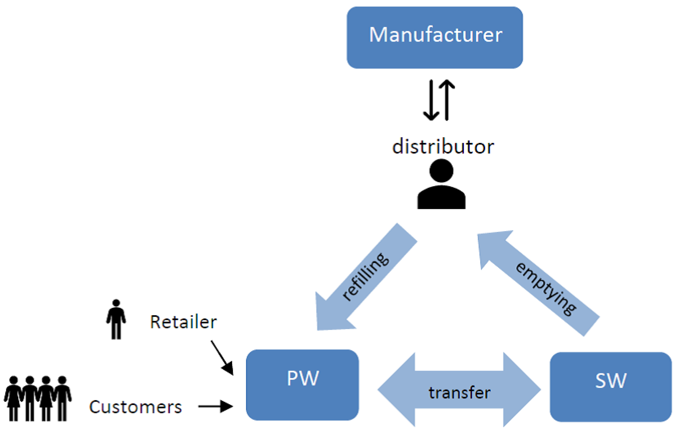
A schematic diagram of the relationship between the existing entities is presented in Figure 1.

Our model is motivated by various practical settings. The first example is taken from the collaboration between firms and farms—specifically, the vegetable marketing firm Chasalat Alei Katif (https://www.aleikatif.org) (27 December 2022), which specializes in growing insect-free, fresh cabbage without using pesticides. The firm markets products from several farms, each with several greenhouses for growing organic cabbage. The ripe cabbage is stored in the PW, which serves both individual customers and retailers. When the stock in the PW falls below a certain level, the farms supply the firm with additional stock, which is time-consuming. However, according to a special agreement, if the supplied cabbages cannot be stored in the PW (due to capacity constraints), they are sliced, and accumulated until they are sold privately by the farms.

The second example is taken from the collaboration between medical centers and university scientists [3]. Here, specialists are responsible for the operation and management of the blood bank. When a lack of blood donations is observed, the associated medical faculty is enlisted to help carry out a rapid and immediate blood donation campaign on campus. Since the capacity of the storage facility is limited, the surplus blood donations are transferred to the university faculty for academic use, after which it cannot be used by patients.

In this paper, we assume the following costs and rewards: (i) a fixed cost for each order; (ii) a cost for each item supplied by the distributor (this cost includes the payment to the distributor for his maintenance services). (iii) If the PW is not refilled due to a high inventory level, the distributor is rewarded for their maintenance services; (iv) a salvage payment for each item transferred from the PW to the SW; and (iv) a loss cost is charged for each unsatisfied item at the PW.

We seek to determine the optimal levels of s and S that minimize the overall discounted cost of managing the warehouses. We further assume a fixed cost to operate the PW and, thus, each item has a negligible storage cost. This assumption has many applications in reality, e.g., in blood inventory management and in organic food storage, where the cost of storing an item is negligible compared to the cost of cooling the storage facility. Moreover, we assume that the distributor arrives after an exponentially distributed lead time. This assumption is practical when the lead time depends on different logistics factors—for example, for a distributor that serves several independent companies that line up as an M/M/1 queue. The time it takes to prepare and deliver the items can be interpreted as a sojourn time that is exponentially distributed. Due to variable delivery times, the company may ask the distributor for a flexible contract that allows for delays or cancellations of outstanding orders.

The policy addressed here expands the band $(S,s)$-type policy. As far as we know, most of the existing studies under the $(S,s)$ control policy consider continuous movements and allows at most unilateral jumps; there are no studies on inventory management that consider a Markov-modulated process with bilateral continuous and jump movements. However, when considering the significant increase in returns and the uncertainty in lead times, allowing double-side changes is more appropriate for modeling inventory management. Fluctuations in inventory levels, where the inventory level not only decreases due to demands but also increases due to returns, make the analysis much more challenging. From a managerial perspective, this difficulty becomes the main driving force behind for an integrated inventory management.

The main contributions of the paper are fourfold: (1) We differ from existing works in the inventory management literature by considering continuous and batch-type bilateral changes, which are both governed by the underlying Markov chain. We further assume phase-distributed batch amounts, given that any nonnegative continuous distribution can be approximated by a phase distribution. By that, we capture the uncertainty of customers’ consumption habits impacted by a fluctuating environment. As a result, our framework can be adapted to a wide range of applications. (2) We extend classic inventory models to include a limited storage capacity and, thus, introduce a simple and practical $(M,S,s)$-type band policy. As in practice, we further assume that the fixed cost is paid at the time that the order is placed, and that the variable cost is paid at the time the PW is refilled. This difference in timing is significantly important and may lead to cost saving. (3) We also contribute to the inventory management literature by implementing the new business concept integrating partnerships for managing the warehouses. (4) Most existing papers employ analytic approaches, such as a dynamic programming approach [4,5] difference-differential equations approach [6] or scale function [7,8]; by contrast, we use a more probabilistic and intuitive approach. We combine the first-step conditioning technique for the expectation, renewal theory and the strong Markov property (which says that, for a Markovian process $X\left(t\right)$, conditioning on state at a given stopping time T, the probabilistic behavior of the process depends only on its value at time T and discards its past behavior; see [2]). By doing so, we build a relatively simple set of equations that provide managers with a useful and efficient tool to derive optimal thresholds. To the best of our knowledge, this is the first time that first-passage time results have been carried out in bilateral movements in the inventory management literature. We further note that many studies deal with the long-run average criterion, without taking timing into consideration [5,9]. Our results show that timing significantly impacts the system performance and is a crucial factor; therefore, it should be taken into account.

From our conclusions, we numerically glean some important insights. Firstly, the total cost seems to be convex in S and s (for a fixed M; see Figure 4. Although we cannot prove this result, it enables us to numerically obtain the optimal thresholds $S^{*}$ and $s^{*}$ using a linear search over the range $0\le s<S<M$. Secondly, we show the impact of the limited capacity of the PW on the optimal thresholds, especially when the transfer cost is high (see Figure 4a, Table 2, and the discussions thereafter). Thirdly, as demands become more frequent, it becomes worthwhile to order more frequently and for smaller quantities. In such a case, the impact on $S^{*}$ is negligible and, surprisingly, the weight of the cost’s components is relatively fixed (here, the transfer cost is negligible). By contrast, more returns prompt the manager to reduce the frequency of orders and enlarge their quantities. Here, the weight of the cost of the distributor’s services increases relative to the weight of the loss cost (see Figures 5–8). Fourthly, investigating the impact of the timing, we observe that, when the discount factor is high, postponing the call for the distributor becomes economically profitable (see Figure 9). The outline of the paper is as follows: In Section 2, we review the related literature. Section 3 presents the mathematical structure of the stock levels at the PW and SW; the cost components are also detailed. The core preliminaries are given in Section 4. Section 5 derives the expected discounted cost components; a summary of the costs’ derivation is given in Appendix A.2. Numerical examples, observations, and insights are provided in Section 6. Finally, Section 7 concludes. Technical parts of the proofs are relegated to Appendix B.1, Appendix B.2 and Appendix B.3.

2. Literature Review

It is well established in the literature that customer flows can exhibit high variability and unpredictably [10,11], state dependency [12], and batch patterns [13,14]. Thus, modeling the behavior of customers has become a key challenge in inventory management. These modeling challenges are aggravated by the rapid spread of the home shopping phenomenon, which force retailers to incorporate the occurrence of returns on a daily basis [4]. Real-word examples of such variability include the introduction of new products, where the flow rates are obviously non-stationary and evolve throughout the stages of the product’s life cycle [15,16], fluctuating environments, where economic conditions, extreme weather, technological advancements, competition, and dynamic events can perturb customer flows [17,18,19], home shopping and internet retailing, where a high return rate, particularly for electronic and computer devices, significantly changes customers’ behavior [20,21]. Any of these sources of variability on its own impacts the on-hand stock level and, thus, complicates the analysis of the inventory model. Therefore, a considerable portion of the related literature usually uses Markov processes due to their versatility in matching key statistical properties of the customers’ consumption needs [10,13,22,23].

In this study, the inventory level changes are the sum of continuous linear rates forming a likewise fluid process, and instantaneous big inflows and outflows governed by a Poisson process. For example, a company that sells its product through two channels, usual daily sell contracts and one-time opportunities [24], or a manufacturer who produces a component needed for few products, as well as a replacement [25]. Consequently, an excellent example of a return in batches policy is out-of-fashion products, and parts delivered to maintenance service engineers, particularly in isolated areas [4].

We assume that the batch sizes come from the family of phase distributions. The advantage of a PH distribution is that its Markovian nature allows for an exact analysis and performance evaluation; thus, they are often used [12,13,26,27]. When general distributions are appropriate, phase distributions can be taken into account in a natural way, as any nonnegative continuous distribution of the probability can be approximated with a phase-type distribution [2].

We note that incorporating continuous rates and instantaneous jumps is well studied also in economics and cash management (e.g., loads and withdrawals), in healthcare management (e.g., daily patients and unexpected disasters), in reliability models (e.g., parts delivered to maintenance service engineers in geographically spread out areas), and in chemical production systems and gas stations. More examples are available in [28,29,30].

In the literature, the $(S,s)$ control policy is one of the most widely used [24]. The optimality of $(S,s)$-type policies has been investigated for various inventory models, including those with discrete and continuous time reviews, different time horizons, discounted or average cost criteria, and backlogging or lost-sales. Under continuous time, the underlying stochastic stock level governing the state variables is typically linked to either varying rates [4,31], fluid processes [32], Wiener processes [9,33,34,35,36], renewal processes [5,12,37,38], superposition of deterministic rates combined with a renewal process [25], and a one-sided Lèvy process [7,39,40]. Using batch-size patterns, Bensoussan et al. [41] consider two models: one model is a mixture of a diffusion process and a compound Poisson process with exponentially distributed jump sizes, and the second model, as in Presman and Sethi [25], is a mixture of constant demand governed by a compound Poisson process. Their work was generalized by Benkherouf and Bensoussan [6] to a general compound Poisson process. Yamazaki [8] tackled the inventory problem when the demand follows a Lèvy process with jumps having infinite activity/variation. Chakravarthy and Rao [42] assume that the customers arrive according to a Markovian arrival process (MAP) with demand of varying sizes. Along with this line, Barron [13,18] studies a mixture of a fluid process and a MAP demand process. For a comprehensive survey, see [24].

All papers cited above consider a one-dimensional inventory process. For the multidimensional process, several models used in the literature focus on the derivation of the Laplace transform of the first-passage time in a Markov-modulated process with bilateral random jumps, mostly for studying various financial problems (e.g., [26,39,43,44,45]).

Furthermore, the increasing environment uncertainty has been mitigated over the last few decades, the phenomenon of a gradual transition to collaborative and integrative approaches to achieving optimal supply chain performance. In this paper, we assume that the distributor also assists with the maintenance and upkeep of the storage. Particularly, it has become customary for managers to motivate high-quality relationships with their distributor. Research on marketing shows that most distributors also provide a range of services such as technical support, warranty, and other complex services [46,47,48].

To outline our position, an overview of the most relevant literature studies concerning the continuous-review base stock policy is given in

Table A1. Selected studies on continuous review base stock inventory policy.

Continuous-Review Base-Stock Inventory Models	Model Features					Optimization Approach
Authors	Arrival Pattern of Demand/Return	Movement Patterns (Conti., Jumps)	Lead Time	Base-Stock Policy	Additional Features
Benkherouf, Bensoussan (2009) [6]	Com. Poiss. + diffusion/no returns	One-sided jumps	zero	(qi, ui)- band policy	Disc. criteria	■ A quasi-variational inequalities approach
Yamazaki (2016, 2017) [8,29]	Spectrally positive Lévy processes	One-sided jumps	zero	(S, s)	Disc. criteria	■ fluctuation theory of Lévy processes ■ The scale function
Perera, Janakiraman, Niu (2018) [5]	Renewal proc./no returns	One-sided unit jumps	zero/ constant	(S, s) (B)	Long run analysis	■ Renewal theory ■ Deterministic dynamic programming
Barron (2018) [18]	Fluid flow /MAP	One-sided jumps	zero	(Q, 0) (LS)	Disc. criteria Obsolescence + emergency	■ Martingales ■ Numerical investigation
Azcue, Muler (2019) [43]	Comp. Poiss./Comp. Poiss.	Two sided jumps	zero	Multi-band structure	Disc. criteria	■ Solution of HJB equation
Pérez, Yamazaki, Bensoussan (2020) [7]	Spectrally positive Lévy processes	One-sided jumps	zero	Periodical replenishments	Disc. criteria	■ The scale function ■ Guess and verify procedure
Barron, Dreyfuss (2021) [4]	Comp. Poiss./Comp. Poiss.	Two-sided jumps. No conti. movements	exp	(S, s) (LS)	Steady-state analysis	■ Markov chain ■ Numerical investigation
Chakravarthy, Rao (2021) [42]	MAP/no returns	One-sided jumps	zero	Random replenishments (LS, B)	Steady-state analysis	■ Matrix-analytic methods
Barron (2022) [13]	Fluid flow or jumps for demands/no returns	One-sided movements	exp	(S, s) + emergencies	Disc. Criteria Immediate emergency	■ LSTs ■ Numerical investigation
This study	MAP/MAP	Bilateral linear rates. Two-sided-PH-Jumps	exp	(M, S, s) (LS)	Disc. Criteria Joint management policy, two storages	■ Renewal set of equations ■ LSTs ■ Multidimensional Martingales ■ Numerical investigation

in Appendix A.1. To the best of our knowledge, the combination of random demands and returns (bilateral continuous and jump type) in supply chain collaboration under the $(S,s)$ policy with cancellation has not been explored in literature of inventory management; hence, the model developed here significantly contributes to the literature.

3. The Stock Level Processes at PW and SW

In this section, we use similar notations to those of Breuer [27] (see also [18,26]).

Consider two storage facilities, the PW and the SW, and two types of customers, namely, individual customers and retailers. The demands (returns) of the individual customers form a likewise fluid process with linear rates, governed by a continuous-time Markov chain (CTMC) that is used as a background environment as follows. Let $\tilde{\mathcal{J}}=\{\tilde{J}\left(t\right):t\ge 0\}$ be a CTMC with state space $\tilde{E},$ initial probability vector $\mathbf{\eta }=\left[{\mathbf{\eta }}_1,{\mathbf{\eta }}_2,\dots ,{\mathbf{\eta }}_{\left|\tilde{E}\right|}\right],$ and infinitesimal generator $\tilde{\mathbb{Q}}={\left({\tilde{q}}_{ij}\right)}_{i,j\in \tilde{E}}.$ Let $\mathbf{\pi }$ be the stationary probability vector; $\mathbf{\pi }$ is the unique solution of the equation $\mathbf{\pi }\tilde{\mathbb{Q}}=0$ such that $\mathbf{\pi }\mathit{E}=1$. When the state equals $i\in \tilde{E}$, products are returned at rate $r_i,$ and demand is observed at rate $d_i$ by the individual customers. The growth rate is denoted by $c_i=r_i-d_i,$ which can be positive or negative. Thus, the state space $\tilde{E}$ is composed of two subsets $\tilde{E}=E_p\cup E_n,$ where $E_p$ includes the increasing states, $E_p=\{i:c_i>0\},$ and $E_n$ includes the decreasing states, $E_n=\{i:c_i<0\}.$ Accordingly, we use the terms ascending (descending) environment when $i\in E_p$ $\left(E_n\right)$.

Next, we describe the retailers’ arrivals. The retailers arrive at random times and form a Poisson process of instantaneous big inflows (returns) or outflows (demands). Specifically, we assume that, when an ascending environment is observed, i.e., when there are more returns than demands, the manager offers retailers the opportunity to demand products, in order to balance the stock level. On the other hand, when a descending environment is observed, i.e., when there are more demands than returns, the manager offers retailers the ability to return products.

For the mathematical description, we define the process $\hat{\mathcal{I}}=\{\hat{I}\left(t\right):t\ge 0\}$ as a special case of a Lèvy process ${\hat{\mathcal{I}}}^{\left(i\right)}$ with a drift $c_i$ (to describe the customers) and a Lèvy measure ${\hat{v}}_i$ (to describe the retailers) during intervals when the phase equals $i\in \tilde{E}$. We assume that ${\hat{v}}_i$ takes the form

$${\hat{v}}_i\left(dx\right)={\lambda }_i^{(+)}{\mathbf{1}}_{\{i\in E_n\}}{\mathbf{\alpha }}^{(i+)}exp\left({\mathbb{T}}^{(i+)}x\right){\mathbf{\eta }}^{(i+)}dx+{\lambda }_i^{(-)}{\mathbf{1}}_{\{i\in E_p\}}{\mathbf{\alpha }}^{(i-)}exp(-{\mathbb{T}}^{(i-)}x){\mathbf{\eta }}^{(i-)}dx,x>0$$

(1)

for all $i\in \tilde{E}.$ Here, ${\lambda }_i^{(\pm )}\ge 0$ is the retailers’ arrival rates, and the retailers’ batch amounts $U^{(i\pm )}$ are PH distributed r.v.s with initial probability vectors ${\mathbf{\alpha }}^{(i\pm )}$ and transition rate matrices ${\mathbb{T}}^{(i\pm )}$; i.e., the arrival process is a compound Poisson process with jump sizes $U^{(i+)}\sim PH\left({\mathbf{\alpha }}^{(i+)},{\mathbb{T}}^{(i+)}\right)$ of order $m_i^{+}$ when $i\in E_n,$ and $U^{(i-)}\sim PH\left({\mathbf{\alpha }}^{(i-)},{\mathbb{T}}^{(i-)}\right)$ of order $m_i^{-}$ when $i\in E_p$. Let ${\mathbf{\eta }}^{(i\pm )}=-{\mathbb{T}}^{(i\pm )}\mathit{e}$ be the exit vectors. Now, the process $\hat{\mathcal{I}}$ is a MAP-modulated process with upward jumps and downward jumps. Let ${\mathbf{\lambda }}^{(+)}$ be a $\left(1\times \left|E_n\right|\right)$ vector whose i component is ${\lambda }_i^{(+)},i\in E_n.$ Similarly, let ${\mathbf{\lambda }}^{(-)}$ be a $\left(1\times \left|E_p\right|\right)$ vector whose i component is ${\lambda }_i^{(-)},i\in E_p$. Finally, define the $\left(1\times {\sum }_{i=1}^{\left|E_n\right|}{m}_i^{+}\right)$ vector ${\mathbf{\alpha }}^{(+)}=\left({\mathbf{\alpha }}^{(1+)},\dots ,{\mathbf{\alpha }}^{(\left|E_n\right|+)}\right),$ and the $\left(1\times {\sum }_{i=1}^{\left|E_p\right|}{m}_i^{-}\right)$ vector ${\mathbf{\alpha }}^{(-)}=\left({\mathbf{\alpha }}^{(1-)},\dots ,{\mathbf{\alpha }}^{(\left|E_p\right|-)}\right).$

The PW is controlled by a triple-parameter band policy $(M,S,s),$ $0\le s<S\le M,$ under a lost sales policy. Let ${\tilde{\mathcal{I}}}_o=\{{\tilde{I}}_o\left(t\right):t\ge 0\}$ be the on-hand stock level at the PW. We assume that, as soon as ${\tilde{\mathcal{I}}}_o$ drops to or below level s, a delivery is ordered and arrives by the distributor after an exponential lead time; during that lead time, new orders are not allowed. When the distributor arrives, if the on-hand stock increases to or above level S, no items are refilled; otherwise, the stock is refilled up to level S. Thus, the amount refilled at arrival time is random and is equal to $max(S-{\tilde{I}}_o\left(t\right),0)\equiv {\left[S-{\tilde{I}}_o\left(t\right)\right]}^{+}$ items. We further assume that the PW has a capacity of $M>S$ units. Every time the inventory exceeds level M, the excess items are transferred from PW to SW in a negligible amount of time and for some fee. Hence, ${\tilde{\mathcal{I}}}_o$ lies in the range $[0,M]$.

Next, we describe the management of the SW. The SW has unlimited capacity. Each time the distributor arrives, he provides some basic maintenance activities and empties the SW; no additional payment is given to him for this work. However, if the PW is not refilled, the distributor is rewarded for his service. Let ${\tilde{\mathcal{I}}}_R=\{{\tilde{I}}_R\left(t\right):t\ge 0\}$ be the on-hand stock level at the SW; Note that, in contrast to ${\tilde{\mathcal{I}}}_o,$ the process ${\tilde{\mathcal{I}}}_R$ is not bounded from above. For simplicity, we further assume that ${\tilde{\mathcal{I}}}_o\left(0\right)=S$ and ${\tilde{\mathcal{I}}}_R\left(0\right)=0$.

Let ${\mathcal{L}}_n,n\ge 1$ be a sequence of i.i.d. $exp\left(\mu \right)$-distributed r.v.s representing the lead times independent of $({\tilde{\mathcal{I}}}_o,\tilde{\mathcal{J}})$. Let ${\mathcal{Z}}_1=inf\{t:t>0,{\tilde{I}}_o\left(t\right)\le s\}$ be the first time that the stock level drops to or below level s, and thus a delivery is ordered. Let $K_1={\mathcal{Z}}_1+{\mathcal{L}}_1$ be the first arrival time of the distributor. We define, recursively, the following stopping times:

$$\begin{array}{cc}{\mathcal{Z}}_n=inf\left\{t:t>{\displaystyle \sum _{i=1}^{n-1}}{K}_i,{\tilde{I}}_o\left(t\right)\le s\right\},\hfill & n=2,3,\dots \hfill \\ K_n={\mathcal{Z}}_n+{\mathcal{L}}_n,\hfill & n=2,3,\dots \hfill \end{array}$$

(2)

The r.v. ${\mathcal{Z}}_n,n=1,2,\dots ,$ represents the n-thorderingtime; the r.v $K_n,n=1,2,\dots$ represents the n-th arrival time of the distributor. Recall that ${\tilde{I}}_o\left({\mathcal{Z}}_n\right)=s$ occurs only due to a continuous hitting linear rate, i.e., by a customer’s demand, while ${\tilde{I}}_o\left({\mathcal{Z}}_n\right)<s$ occurs due to a downward jump, i.e., by a retailer’s demand. At arrival times, ${\left[S-{\tilde{I}}_o\left(K_n\right)\right]}^{+}$ items are refilled, such that, if ${\tilde{I}}_o\left(K_n\right)<S,$ then ${\tilde{I}}_o$ is refilled with $S-{\tilde{I}}_o\left(K_n\right)$ items and starts from level S; otherwise, no refilling is carried out. In addition, at times $K_n,n=1,2,\dots ,$ the SW is emptied. Thus, we have ${\tilde{I}}_o\left(K_n\right)\ge S,{\tilde{I}}_R\left(K_n\right)=0,n=1,2,\dots$. Finally, we define $j_i$ as

$$j_i=min\{K_n>j_{i-1}:{\tilde{I}}_o(K_n-)<S),n=1,2,\dots \},i=1,2,\dots ,\mathrm{with}{j}_0=0,$$

(3)

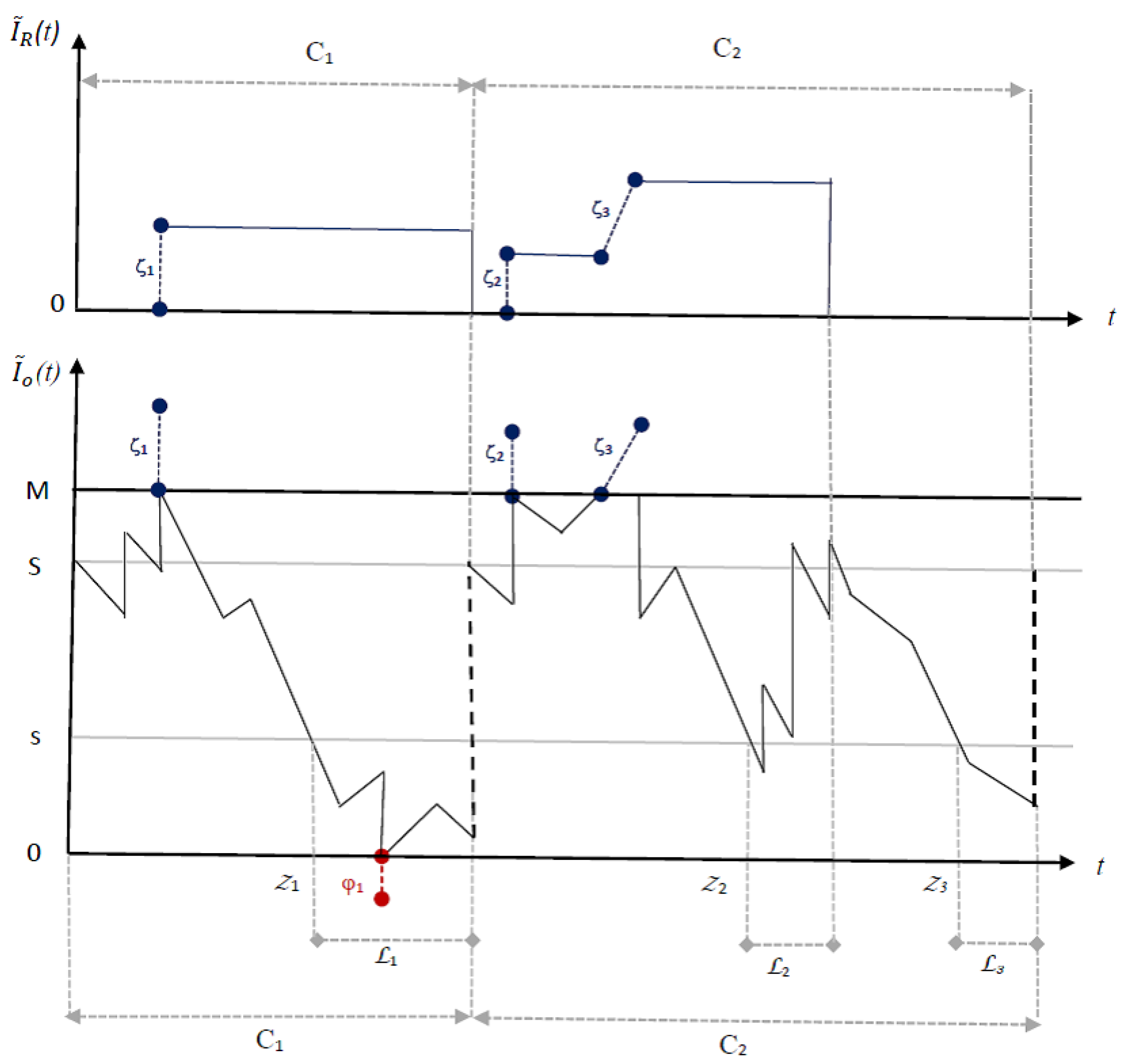
to represent the i-th (actual) refilling time of the PW (and emptying time of the SW). Clearly, we obtain ${\tilde{I}}_o\left(j_i\right)=S$ and ${\tilde{I}}_R\left(j_i\right)=0$ for $i=1,2,\dots$. It is easy to verify that the processes ${\tilde{I}}_o\left(t\right)$ and ${\tilde{I}}_R\left(t\right),t\ge 0$ are semi-regenerative processes with regenerative points $j_i,i=1,2,\dots$ Let ${\mathcal{C}}_i=j_i-j_{i-1},$ $i=1,2,\dots$ be the time between two consecutive (actual) refillings. A typical sample path of ${\tilde{I}}_o\left(t\right)$ and ${\tilde{I}}_R\left(t\right)$ is depicted in Figure 2.

The stock levels of PW and SW, ${\tilde{I}}_o\left(t\right)$ and ${\tilde{I}}_R\left(t\right),$ are depicted in the bottom and top parts of Figure 2, respectively. We start with the first cycle. At time ${\mathcal{Z}}_1,$ we have ${\tilde{I}}_o\left({\mathcal{Z}}_1\right)<s,$ and thus a delivery is ordered. After lead time ${\mathcal{L}}_1,$ when the distributor arrives, ${\tilde{I}}_o(K_1={\mathcal{Z}}_1+{\mathcal{L}}_1)<S,$ and thus the refilling is carried out, the stock is raised up to level $S,$ and the cycle ends. At that time, the SW is emptied by the distributor. Here, $j_1=K_1.$ By contrast, during the second cycle, a delivery is ordered twice. At the first time, ${\mathcal{Z}}_2,$ the distributor arrives after lead time ${\mathcal{L}}_2$ when ${\tilde{I}}_o(K_2={\mathcal{Z}}_2+{\mathcal{L}}_2)>S,$ and thus no items are supplied and only maintenance service is performed, leading to ${\tilde{I}}_R\left(K_2\right)=0.$ The second order is placed at time ${\mathcal{Z}}_3,$ when ${\tilde{I}}_o\left({\mathcal{Z}}_3\right)<s.$ Here, we see that ${\tilde{I}}_o(K_3={\mathcal{Z}}_3+{\mathcal{L}}_3)<S,$ and thus the PW is refilled, the SW is emptied, and the cycle ends. Here, $j_2=K_3$ and we obtain ${\tilde{I}}_o\left(j_2\right)=S$ and ${\tilde{I}}_R\left(j_2\right)=0.$ Figure 2 also shows that level M is exceeded three times: once during cycle 1 with ${\zeta }_1$ items (due to a return by a retailer), and twice during cycle 2 with ${\zeta }_2$ (due to return by a retailer) and with ${\zeta }_3$ items (due to a return by a customer); these overstocking events are represented by the blue segments. The excess items are accumulated in the SW and emptied at times $K_1$ and $K_2$ (we note that maintenance services are also provided at time $K_3={\mathcal{Z}}_3+{\mathcal{L}}_3;$ however, since ${\tilde{I}}_o\left(t\right)<M$ and ${\tilde{I}}_R\left(t\right)=0$ for $t\in (K_2,K_3],$ no change in ${\tilde{I}}_R$ is depicted in the figure). In addition, we see one shortage event, with amounts of ${\phi }_1$ (due to a demand by a retailer), represented by the red segment.

Our aim is to find the optimal parameters in order to optimize the expected discounted total cost. To that end, we let ${\mathbb{E}}_x\left(e^{-\beta C}\right)$ be the $\left(\left|\tilde{E}\right|\times \left|\tilde{E}\right|\right)$ conditional Laplace transform matrix (LST) of the cycle length whose $(i,j)$-th component is:

$${\left({\mathbb{E}}_x\left(e^{-\beta C}\right)\right)}_{i,j}=E(e^{-\beta C}{1}_{\{\tilde{J}\left(C\right)=j\}}\mid {\tilde{I}}_o\left(0\right)=x,\tilde{J}\left(0\right)=i),i,j\in \tilde{E}.$$

Applying renewal theory, we can express all the cost functionals by using the first cycle.

(a) Order cost $OC\left(\beta \right)$. At ordering time, a fixed cost ${{\rm Y}}^{{}^{+}}$ is paid. This cost is non-refundable (even when no refilling is performed due to returns). Note that there may be multiple orders per cycle, each costing ${{\rm Y}}^{{}^{+}}$. Thus, we obtain

$$OC\left(\beta \right)={{\rm Y}}^{{}^{+}}\sum _n{E}_S\left(e^{-\beta {\mathcal{Z}}_n}\right)={{\rm Y}}^{{}^{+}}\mathbf{\eta }{\left(\mathbb{I}-{\mathbb{E}}_S\left(e^{-\beta C}\right)\right)}^{-1}{\mathit{O}\mathit{C}}_S\left(\beta \right),$$

(4)

where ${\mathit{O}\mathit{C}}_S\left(\beta \right)$ is the $(\left|\tilde{E}\right|\times 1)$ vector, representing the total expected discounted ordering times per cycle, given ${\tilde{I}}_o\left(0\right)=S,\tilde{J}\left(t\right)\in \tilde{E}.$

(b) Distributor’s service cost.At times $j_n,n=1,2,\dots$, the PW is refilled with $S-{\tilde{I}}_o(j_n-)$ items and the cycle ends; this amount is random depending on the stock level upon arrival. Let $\gamma$ be the cost of each refilled item (and is charged when the distributor arrives). When no refilling is performed, the distributor is rewarded with ${{\rm Y}}^{{}^{-}}$ for his maintenance services. Summarizing, we obtain

$$\begin{array}{cc}\hfill DC\left(\beta \right)& =\gamma \sum _n{E}_S\left(e^{-\beta j_n}(S-{\tilde{I}}_o\left(j_n\right))\right)+{{\rm Y}}^{{}^{-}}\sum _n{E}_S\left(e^{-\beta K_n}{\mathbf{1}}_{\{{\tilde{I}}_o\left(K_n\right)>S\}}\right)\hfill \\ \hfill & =\gamma ·S\sum _n{E}_S\left(e^{-\beta C_n}\right)+\sum _n{E}_S\left(e^{-\beta K_n}\right)\left({{\rm Y}}^{{}^{-}}{\mathbf{1}}_{\{{\tilde{I}}_o\left(K_n\right)>S\}}-\gamma {\tilde{I}}_o\left(K_n\right){\mathbf{1}}_{\{{\tilde{I}}_o\left(K_n\right)<S\}}\right)\hfill \\ \hfill & =\mathit{\eta }{\left[\mathbb{I}-{\mathbb{E}}_S\left(e^{-\beta C}\right)\right]}^{-1}{\mathit{D}\mathit{C}}_S\left(\beta \right),\hfill \end{array}$$

(5)

where ${\mathit{D}\mathit{C}}_S\left(\beta \right)$ is the expected discounted cost per cycle incurred by the distributor. Note that, while ${{\rm Y}}^{{}^{-}}$ may be charged several times per cycle (due to maintenance services), $\gamma$ is charged only once, at the end of the cycle, when the PW is refilled.

(c)Transfer cost $SC\left(\beta \right)$. When the on-hand stock in the PW exceeds level $M,$ the excess amount is transferred to the SW. Let $\nu$ be the cost of transferring each item. Here, level M is exceeded either continuously by an individual customer at a linear rate $c_{\tilde{J}\left(t\right)},$ $\tilde{J}\left(t\right)\in E_p$, or by an upward jump due to a demand by a retailer. In the latter case, denote by ${\Xi }_n$ the n-th time that level M is exceeded by an upward jump, and let ${\zeta }_n$ be the amount exceeding level M and transferred to SW at time ${\Xi }_n$. The overall discounted transfer cost is given by (see also Remark 1, Point 1):

$$\begin{array}{cc}\hfill SC\left(\beta \right)& =v\left(\sum _{n=1}^{\infty }E\left(e^{-\beta {\Xi }_n}{\zeta }_n\right)+\underset{0}{\overset{\infty }{\int }}E\left(e^{-\beta t}{c}_{\tilde{J}\left(t\right)}{\mathbf{1}}_{\{{\tilde{I}}_o\left(t\right)=M,\tilde{J}\left(t\right)\in E_p\}}\right)dt\right)\hfill \\ \hfill & =\mathit{\eta }v{\left(\mathbb{I}-\mathbb{E}\left(e^{-\beta C}\right)\right)}^{-1}{\mathit{S}\mathit{C}}_S\left(\beta \right),\hfill \end{array}$$

(6)

where the $(\left|\tilde{E}\right|\times 1)$ vector ${\mathit{S}\mathit{C}}_S\left(\beta \right)$ is the expected discounted amount exceeding level M per cycle. Note that the first (second) term of (6) refers to a jump (continuous linear rate).

(d) Loss cost $LC\left(\beta \right)$. Any demand or part of a demand that is not satisfied is lost. Similarly, we distinguish between customers and retailers. Level 0 is hit either continuously by an individual customer at a linear rate $-c_{\tilde{J}\left(t\right)},\tilde{J}\left(t\right)\in E_n,$ or by a retailer by a downward jump. Let ${\Phi }_n$ be the n-th time that level 0 is hit by a downward jump, and let ${\phi }_n$ be the number of unsatisfied demands at time ${\Phi }_n$. Let $\varphi$ be the cost of each unsatisfied demand. The expected discounted loss cost is given by (see also Remark 1, Points 1 and 2):

$$\begin{array}{cc}\hfill LC\left(\beta \right)& =\varphi \left(\sum _{n=1}^{\infty }E\left(e^{-\beta {\Phi }_n}{\phi }_n\right)-\underset{0}{\overset{\infty }{\int }}E\left(e^{-\beta t}{c}_{\tilde{J}\left(t\right)}{\mathbf{1}}_{\{{\tilde{I}}_O\left(t\right)=0,\tilde{J}\left(t\right)\in E_n\}}\right)dt\right)\hfill \\ \hfill & =\mathit{\eta }\varphi {\left(\mathbb{I}-{\mathbb{E}}_S\left(e^{-\beta C}\right)\right)}^{-1}{\mathit{L}\mathit{C}}_S\left(\beta \right),\hfill \end{array}$$

(7)

where the $(\left|\tilde{E}\right|\times 1)$ vector ${\mathit{L}\mathit{C}}_S\left(\beta \right)$ is the expected discounted unsatisfied demands per cycle.

Remark 1. 

• Regarding the individual customers. We emphasize that, when the on-hand stock level M is exceeding in an ascending state $i\in E_p$, demands are continuously satisfied by some of the returns (and the remaining returns are transferred to the SW at rate $c_i=r_i-d_i>0$). Similarly, when the on-hand stock level 0 is hit in a descending state $i\in E_n$, some of the demands are continuously satisfied by returns (and the remaining unsatisfied demands are lost at rate $-c_i>0$).
• As in practice, here we assume that new arrivals (both customers and retailers) are willing to accept that only some of their demands are satisfied as long as they receive some compensation for the unsatisfied demands. Nowadays, such a policy is highly valued and and even considered by the customer as a high level of service.

The expected total cost of integrated inventory management is therefore

$$TC\left(\beta \right)=OC\left(\beta \right)+DC\left(\beta \right)+SC\left(\beta \right)+LC(\beta ).$$

In what follows, we denote by ${\left(\mathbb{A}\right)}_{ij}$ the elements of a matrix $\mathbb{A},$ by ${\mathbb{A}}_{{}_i{,}_j}$ the submatrix of $\mathbb{A}$ with row indices in $E_i$ and column indices in $E_j;$ in particular, the matrix ${\mathbf{0}}_{i,j}$ represents the $(\left|E_i\right|\times \left|E_j\right|)$ zero matrix. Vectors are denoted by bold letters (e.g., $\mathit{E},\mathit{P}$), and matrices by blackboard letters (e.g., $\mathbb{E},\mathbb{P}$). The $(\left|E\right|\times \left|E\right|)$ conditional matrix expectation, given an initial state $(x,i\in E),$ is denoted by ${\mathbb{E}}_x(.)=\mathbb{E}(.\mid I\left(0\right)=x)$ (and, similarly, the $(\left|E\right|\times 1)$ conditional vector expectation ${\mathit{E}}_x(.)$). Specifically, we use the notations ${\overline{\mathbb{E}}}_x(.)$ and ${\underline{\mathbb{E}}}_x{(.)}^T$ to denote the submatrices of ${\mathbb{E}}_x(.),$ of order $(\left|E_p\right|\times \left|E\right|)$ and $(\left|E_n\right|\times \left|E\right|),$ respectively, associated with the ascending and the descending states of ${\mathbb{E}}_x(.)$, i.e., ${\mathbb{E}}_x(.)={\left({\overline{\mathbb{E}}}_x(.),{\underline{\mathbb{E}}}_x(.)\right)}^T$. Following convention, we let $1_{\left\{A\right\}}$ be the indicator of an event $A,$ $\mathit{e}={(1,\dots ,1)}^T$ be the unit column vector, and $(A$ $B)$ be the matrix obtained by stringing the matrix B after the matrix A, all of the appropriate size.

4. Preliminaries

4.1. Markov-Modulated Fluid Flow Process for MAP

Following Breuer [27], let $\tilde{\mathcal{J}}=\{\tilde{J}\left(t\right),t\ge 0\}$ be a CTMC with state space $\tilde{E}$ and infinitesimal generator $\tilde{\mathbb{Q}}={\left({\tilde{q}}_{ij}\right)}_{i,j\in \tilde{E}}$. Let $\hat{\mathcal{I}}=\{\hat{I}\left(t\right),t\ge 0\}$ be a real-valued process evolving like a Lévy process ${\hat{\mathcal{I}}}^{\left(i\right)}$ with a drift $c_i$ (negative or positive) and a Lévy measure ${\hat{v}}_i$ (given by (1)) when $i\in \tilde{E};$ here, we assume a compound Poisson jump. The jump sizes $U^{(i\pm )}$ are PH-distributed r.v.s $PH\left({\mathbf{\alpha }}^{(i\pm )},{\mathbb{T}}^{(i\pm )}\right)$ of order $m_i^{\mp }$ and depend on the phases $i\in \tilde{E}$ prior to the jumps. The two-dimensional process $(\hat{\mathcal{I}},\tilde{\mathcal{J}})$ is called a MAP. The main advantage of PH-distributed jumps is the possibility of lengthening the jumps into a succession of linear periods of exponential duration (having slopes 1 and $-1$ for the positive and negative jumps, respectively) and retrieving the original process via a simple time change. The transformation is conducted as follows. First, we partition the phase space $\tilde{E}$ (without the jumps) into subspaces $E_p$ (for positive drifts, i.e., $c_i>0$) and $E_n$ (for negative drifts, i.e., $c_i<0$), $\tilde{E}=E_p\cup E_n$. Then, we introduce two new phase spaces:

$$E_{\pm }:=\{(i,k,\pm ):i\in \tilde{E},1\le k\le m_i^{\pm }\},$$

(8)

to model the (positive and negative) jumps. Next, we define the enlarged state space $E\equiv \tilde{E}\cup E_{-}\cup E_{+}$. The revised phase process $\mathcal{J}$ with state space E is determined by the generator matrix $\mathbb{Q}={\left(q_{ij}\right)}_{i,j\in E}$

$$q_{ij}=\left\{\begin{array}{cc}{\tilde{q}}_{ii}-{\lambda }_i,\hfill & j=i\in \tilde{E},\hfill \\ {\tilde{q}}_{ij},\hfill & j\ne i,h\in \tilde{E},\hfill \\ {\lambda }_i{\alpha }_k^{(i\pm )},\hfill & j=(i,k,\pm ),\hfill \end{array}\right.$$

(9)

for $i\in \tilde{E}$ as well as

$$q_{(i,k,\pm ),(i,l,\pm )}=T_{kl}^{(i\pm )}\mathrm{and}{q}_{(i,k,\pm ),i}={\mathbf{\eta }}_k^{(i\pm )}$$

(10)

for $i\in \tilde{E}$ and $1\le k,l\le m_i^{\pm }.$ By that, $\mathcal{J}$ tracks the states (phases) of the PH-type jumps in addition to the states in $\tilde{\mathcal{J}}.$ The revised process constructed by such a technique is denoted by $\{\mathcal{I},\mathcal{J}\}$ and becomes a Markov-modulated fluid flow process (MMFF) without jumps. Accordingly, the infinitesimal generator $\mathbb{Q}$ can be written in block form with respect to the subspaces $E_1=E_p\cup E_{+}$ (ascending states) and $E_2=E_n\cup E_{-}$ (descending states):

$$\mathbb{Q}=\left(\begin{array}{cc}{\mathbb{Q}}_{11}\hfill & {\mathbb{Q}}_{12}\hfill \\ {\mathbb{Q}}_{21}\hfill & {\mathbb{Q}}_{22}\hfill \end{array}\right).$$

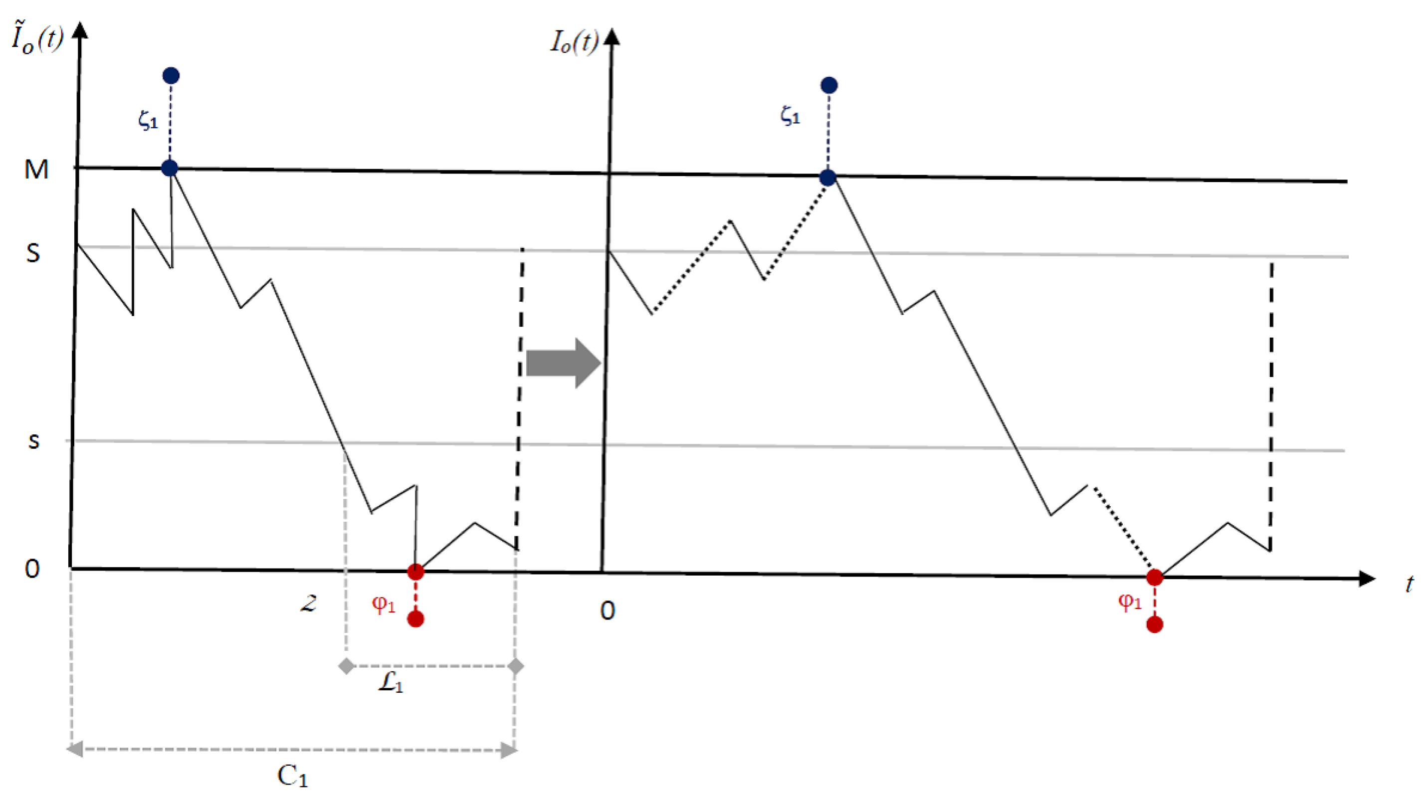
Specifically, we modify the MAP $\{{\tilde{\mathcal{I}}}_o,\tilde{\mathcal{J}}\},$ with ${\tilde{\mathcal{I}}}_o$ being the stock level at the PW, to the revised MMFF process $\{{\mathcal{I}}_o,\mathcal{J}\}.$ Figure 3 illustrates the first cycle of ${\tilde{\mathcal{I}}}_o,$ presented in Figure 2, and its corresponding sample path ${\mathcal{I}}_o$; the jumps that are lengthened to linear segments are marked by the dotted black segments. Note that downward jumps below level 0 and upward jumps above level M are preserved in their original form and are not lengthened to linear segments (as we will show, these quantities require a special treatment). Next, we present the main tools used for the analysis of the MMFF process $\{{\mathcal{I}}_o,\mathcal{J}\}$.

4.2. First-Passage Times

In our analysis, the Laplace transform matrices of the first passage times play an essential component. Our first step is to obtain the LST matrix $\mathbb{A}\left(\beta \right)$ of the return time for the MAP $\{{\tilde{\mathcal{I}}}_o,\tilde{\mathcal{J}}\}$ process. Using $\mathbb{A}\left(\beta \right)$ as a key matrix, we then obtain the conditional LST matrices of the first passage times for the MMFF process.

4.2.1. Return Times for MAPs

Let $\{\tilde{I}\left(t\right),\tilde{J}\left(t\right),t\ge 0\}$ be a MAP process with phase-type jumps. Define $\tilde{\tau }\left(x\right)=inf\{t\ge 0,\tilde{I}\left(t\right)>x\}$ for $x\ge 0$ to be the LST of the first passage time above x. Assume that $\tilde{I}\left(0\right)=0$ and let

$$E_{ij}\left(e^{-\beta \tilde{\tau }\left(x\right)}\right)=E(e^{-\beta \tilde{\tau }\left(x\right)},J\left(\tau \left(x\right)\right)=j\mid \tilde{I}\left(0\right)=0,\tilde{J}\left(0\right)=i),i,j\in E.$$

(11)

Breuer [27] shows that the matrix $\mathbb{E}\left(e^{-\beta \tilde{\tau }\left(x\right)}\right)$ can be written in a block form according to $E_1$ and $E_2$ as

$$\mathbb{E}\left(e^{-\beta \tilde{\tau }\left(x\right)}\right)=\left(\begin{array}{cc}{e}^{\mathbb{U}\left(\beta \right)x}\hfill & \mathbf{0}\hfill \\ \mathbb{A}\left(\beta \right)e^{\mathbb{U}\left(\beta \right)x}\hfill & \mathbf{0}\hfill \end{array}\right),$$

(12)

for some matrices $\mathbb{U}\left(\beta \right)$ and $\mathbb{A}\left(\beta \right)$ of dimensions $\left|E_1\right|\times \left|E_1\right|$ and $\left|E_2\right|\times \left|E_1\right|,$ respectively (note that, since a first passage to a level above cannot occur at a descending state, we have the zero matrices). Furthermore, the matrices $\mathbb{U}\left(\beta \right)$ and $\mathbb{A}\left(\beta \right)$ can be determined by successive approximation to the limits of the sequence $((A_n,U_n):n\ge 0)$ with specific initial values (see Section 2.2 of Breuer [27] for the detailed algorithm). Setting $x=0$ in (11) and (12)$,$ i.e., the return time to level 0 from below given $\tilde{I}\left(0\right)=0,$ yields that ${\mathbb{E}}_{11}\left(e^{-\beta \tilde{\tau }\left(0\right)}\right)=\mathbb{I}$ and ${\mathbb{E}}_{21}\left(e^{-\beta \tilde{\tau }\left(0\right)}\right)=\mathbb{A}\left(\beta \right).$

An important variant of the MAP process $\tilde{\mathcal{I}},$ called the image-reversedprocess,is particularly useful in the analysis of our process. We define the image-reversed MAP process ${\tilde{\mathcal{I}}}^r$ by reversing the roles of the up and down states; let ${\tilde{\mathcal{J}}}^r\left(t\right)$ be the modulated state process for ${\tilde{\mathcal{I}}}^r$. Then, ${\mathbb{A}}^r\left(\beta \right)$ is the matrix of order $\left(\left|E_1\right|\times \left|E_2\right|\right),$ whose $\left(i,j\right)$-th component is the LST of ${\tilde{\tau }}^r\left(0\right),$ i.e., the time until a downward jump to level 0 for the process ${\tilde{\mathcal{I}}}^r$ at state $j\in E_2$, given that ${\tilde{I}}^r\left(0\right)=0$ and ${\tilde{\mathcal{J}}}^r\left(0\right)=i\in E_1$. As we show, these two LSTs, $\mathbb{A}\left(\beta \right)$ and ${\mathbb{A}}^r\left(\beta \right),$ are the key matrices used in our analysis; we further emphasize that these matrices are the return time for the original MAP process, meaning that the time spent in jump states $E_{\pm }$ does not account.

Next, to extend our LSTs and include upper and lower borders, we employ results from MMFF processes.

4.2.2. First Passage Times for MMFF Processes

Let ${}_u^v\tau (x,y)$ (for $x\ge 0,y\ge 0$) be the first passage time of $\mathcal{I}$ from level x to level $y,$ with avoiding a visit to the levels in $[0,u]\cup [v,\infty )$ enroute (in the case of an unlimited visit, u and v are omitted). The notation ${}_u^v\hat{f}(x,y,\beta )$ denotes the LST matrix of the joint distribution of the first passage time ${}_u^v\tau (x,y)$ and the state of the phase process at that time, ${}_u^v\hat{f}{}^r(x,y,\beta )$ denotes the LST of the hitting time for ${\mathcal{I}}^r$. Ramaswami [49] shows that, once $\mathbb{A}\left(\beta \right)$ and ${\mathbb{A}}^r\left(\beta \right)$ are computed, the derivation of other LST matrices is straightforward; thus, all quantities of interest in this paper are characterized explicitly in terms of $\mathbb{A}\left(\beta \right)$ and ${\mathbb{A}}^r\left(\beta \right)$; the explicit expressions of the LST matrices and their probabilistic interpretations are summarized in [49]. To account for the jump-like nature of the additional movements, we substitute $\beta =0$ in all entries of the form $(i,h),(h,i),$ or $(h,h^{\prime })$ for $i\in \tilde{E}$ and $h,h^{\prime }\in E_{+}\cup E_{-}$. This means that the time is not discounted for all states associated with the jumps (i.e., at states $E_{+}$ and $E_{-}$). Henceforth, we assume that all LST matrices for hitting times ($\mathbb{A}\left(\beta \right),$ ${\mathbb{A}}^r\left(\beta \right),$ ${}_u^v\hat{f}(x,y,\beta )$ and ${}_u^v\hat{f}{}^r(x,y,\beta )$) are modified for the original process $\{{\tilde{\mathcal{I}}}_o,\tilde{\mathcal{J}}\}$.

4.3. MMFF at an Exponential Time

Corollary 1. 

Let $\{\mathcal{I},\mathcal{J}\}$ be an MMFF with state space E and $\mathbb{Q},$ and let $\mathcal{L}$ be an exponential r.v. with rate $\mu >0$ independently of $\{\mathcal{I},\mathcal{J}\}$.

(1)

The LST matrix at time $\mathcal{L}$ with the $\left(ij\right)$-th component

$${\left(\mathbb{E}\left(e^{-\beta \mathcal{L}}\right)\right)}_{ij}=E\left(e^{-\beta \mathcal{L}},J\left(\mathcal{L}\right)=j\mid J\left(0\right)=i\right),i\in E$$

is given by

$$\mathbb{E}\left(e^{-\beta \mathcal{L}}\right)=\mu ((\beta +\mu )\mathbb{I}-\mathbb{Q}{)}^{-1}.$$

(13)

In our analysis, the matrix form of (13) is required in order to track the initial and final states of the background CTMC. Here, we use the fact that, for a CTMC $\mathcal{J}$, the matrix $\mathbb{Q}$ satisfies ${\left(e^{\mathbb{Q}x}\right)}_{ij}=P(J\left(x\right)=j\mid J\left(0\right)=i)$ (see [2]). (Recall that the original state space is $\tilde{E};$ thus, only rows in $\tilde{E}$ are considered while other rows in (13) are set to zero.)

(2)

Applying the complete probability equation, it is easy to verify that, for a nonnegative generally distributed r.v. $X,$

$$\begin{array}{cc}\hfill \left(i\right)& \mathbb{E}\left(e^{-\beta X}{\mathbf{1}}_{\{X<\mathcal{L}\}}\right)=\mathbb{E}\left(e^{-(\beta +\mu )X}\right).\hfill \\ \hfill \left(ii\right)& \mathbb{E}\left(e^{\mathbf{\alpha }I\left(\mathcal{L}\right)-\beta L}{\mathbf{1}}_{\{\mathcal{L}<X\}}\right)=\mu \mathbb{E}\left(\underset{t=0}{\overset{X}{\int }}{e}^{\mathbf{\alpha }I\left(t\right)-\left(\beta +\mu \right)t}dt\right).\hfill \end{array}$$

(14)

Here, Equations (13) and (14) are used with respect to the lead time $\mathcal{L}$.

4.4. The Multidimensional Martingale

Let $\left\{\mathcal{X}\right(t),t\ge 0\}$ be a right-continuous Markov-modulated Lévy process with a modulating process $\left\{\mathcal{J}\right(t),t\ge 0\}$ that is an irreducible right-continuous Markov chain with a finite state space E. Let $\left\{Y\left(t\right),t\ge 0\right\}$ be an adapted continuous process with a finite expected variation on finite intervals and let $\mathcal{Z}\left(t\right)=\mathcal{X}\left(t\right)+Y\left(t\right).$ Asmussen and Kella [50] have shown that the matrix with elements $E_i\left[e^{\alpha \mathcal{X}\left(t\right)};J\left(t\right)=j\right]$ has the form of $e^{t\mathbb{K}\left(\alpha \right)}$ for some matrix $\mathbb{K}\left(\alpha \right).$ Theorem 2.1 of Asmussen and Kella [50] yields that, under certain mild conditions on $\left\{\mathcal{Z}\left(t\right),t\ge 0\right\},$ the multidimensional process

$$\mathbf{M}(\alpha ,t)={\int }_{u=0}^t{e}^{\mathbf{\alpha }\mathcal{Z}\left(u\right)}{\mathbf{1}}_{J\left(u\right)}du\mathbb{K}\left(\alpha \right)+e^{\alpha \mathcal{Z}\left(0\right)}{\mathbf{1}}_{J\left(0\right)}-e^{\alpha \mathcal{Z}\left(t\right)}{\mathbf{1}}_{J\left(t\right)}+\alpha {\int }_{u=0}^t{e}^{\alpha \mathcal{Z}\left(u\right)}{\mathbf{1}}_{J\left(u\right)}dY\left(u\right)$$

(15)

is a (row) vector-valued zero mean martingale. Here, the indicator ${\mathbf{1}}_{J\left(t\right)}$ is an $\left|E\right|$-row vector mean $\{{\mathbf{1}}_{J\left(t\right)=i},i\in E\}$. In our model, the process $I_o\left(t\right)$ has piecewise linear sample paths (at rate $c_i$ for $i\in \tilde{E},$ rate 1 for $i\in E_{+},$ and rate $-1$ for $i\in E_{-}$). Some of the cost functionals used are obtained by applying the optional stopping theorem (OST) to the multidimensional martingale process (15).

5. Derivation of the Expected Discounted Cost Functionals

We need to derive ${\mathit{E}}_S\left(e^{-\beta C}\right),$ ${\mathit{OC}}_S\left(\beta \right),$ ${\mathit{DC}}_S\left(\beta \right),{\mathit{SC}}_S\left(\beta \right),$ and ${\mathit{LC}}_S\left(\beta \right).$ The derivation of ${\mathit{DC}}_S\left(\beta \right)$ is more challenging and will be carried out at the end. To this end, we first derive two unique LSTs associated with hitting the boundaries, i.e., hitting level M from below, and dropping to level 0 from above.

Corollary 2. 

(i)

Assume that level M is hit from below at ascending state $J\left(t\right)\in E_1.$ It is easy to verify that the $(\left|E_1\right|\times \left|E_2\right|)$ matrix ${(\beta \mathbb{I}-{\mathbb{Q}}_{11})}^{-1}{\mathbb{Q}}_{12}$ is the expected discounting time until exiting level M at a descending state (either continuously at a state in $E_n$ or by a downward jump at a state in $E_{-}$). As we set $\beta =0$ in all entries in $E_{+}\in E_1$ due to the jumps, the matrix ${(\beta \mathbb{I}-{\mathbb{Q}}_{11})}^{-1}{\mathbb{Q}}_{12}$ has the block form

$${(\beta \mathbb{I}-{\mathbb{Q}}_{11})}^{-1}{\mathbb{Q}}_{12}=\left(\begin{array}{cc}\hfill {(\beta \mathbb{I}-{\tilde{\mathbb{Q}}}_{11})}^{-1}{\tilde{\mathbb{Q}}}_{12}& (\beta \mathbb{I}-{\tilde{\mathbb{Q}}}_{11}){\mathit{\lambda }}^{(-)}{\mathbf{\alpha }}^{(-)}\\ \hfill \mathbb{I}\otimes \mathit{e}\hfill & \mathbf{0}\end{array}\right)$$

with respect to the subspaces $(E_p$ $E_{+})\times (E_n$ $E_{-})$. The matrix $\mathbb{I}\otimes \mathit{e}$ arises due to the zero time spent in $E_{+},$ and thereafter $I_o\left(t\right)$ immediately returns to its original state in $E_n$ (recall that an upward jump is allowed only when $J\left(t\right)\in E_n)$.

(ii)

Similarly, assume that level 0 is hit from above at a descending state $J\left(t\right)\in E_2$. It is easy to verify that the $(\left|E_2\right|\times \left|E_1\right|)$ matrix ${(\beta \mathbb{I}-{\mathbb{Q}}_{22})}^{-1}{\mathbb{Q}}_{21}$ is the expected discounting time until exiting level 0 at ascending state $E_n$ (either continuously at a state in $E_p$ or by an upward jump at a state in $E_{+}$) Here, too, by setting $\beta =0$ in all entries in $E_{-}\in E_2,$ the matrix ${(\beta \mathbb{I}-{\mathbb{Q}}_{22})}^{-1}{\mathbb{Q}}_{21}$ has the block form

$${(\beta \mathbb{I}-{\mathbb{Q}}_{22})}^{-1}{\mathbb{Q}}_{21}=\left(\begin{array}{cc}\hfill {(\beta \mathbb{I}-{\tilde{\mathbb{Q}}}_{22})}^{-1}{\tilde{\mathbb{Q}}}_{21}& (\beta \mathbb{I}-{\tilde{\mathbb{Q}}}_{22}){\mathit{\lambda }}^{(+)}{\mathbf{\alpha }}^{(+)}\\ \hfill \mathbb{I}\otimes \mathit{e}\hfill & \mathbf{0}\end{array}\right)$$

with respect to the subspaces $(E_n$ $E_{-})\times (E_p$ $E_{+})$.

5.1. Cycle Length and Order Cost

The cycle length is composed of two sequential periods: the time elapsed until level s is hit when a refilling is ordered, and the remaining cycle time. The next proposition summarizes the derivation of ${\mathit{E}}_S\left(e^{-\beta C}\right)$ (recall that the superscript o indicates the stock-level evolution during lead time).

Proposition 1. 

The LST $\left(\left|E\right|\times 1\right)$ vector ${\mathit{E}}_S\left(e^{-\beta C}\right)={\left({\overline{\mathit{E}}}_S\left(e^{-\beta C}\right){\underline{\mathit{E}}}_S\left(e^{-\beta C}\right)\right)}^T$ satisfies the following set of equations:

(remaining cycle length with no upcoming refill)

$$\begin{array}{cc}\hfill \left(i\right){\overline{\mathit{E}}}_S\left(e^{-\beta C}\right)& ={}^{M-S}{\mathbb{A}}^r\left(\beta \right){\underline{\mathbb{E}}}_S\left(e^{-\beta C}\right)+{}_S{\hat{f}}_{11}(S,M,\beta ){\overline{\mathit{E}}}_M\left(e^{-\beta C}\right),\hfill \\ \hfill \left(ii\right){\underline{\mathit{E}}}_S\left(e^{-\beta C}\right)& ={}^S{\hat{f}}_{22}(S,s,\beta ){\underline{\mathit{E}}}_s^o\left(e^{-\beta C}\right)+{}^{S-s}\mathbb{A}\left(\beta \right){\overline{\mathit{E}}}_S\left(e^{-\beta C}\right),\hfill \\ \hfill \left(iii\right){\overline{\mathit{E}}}_M\left(e^{-\beta C}\right)& ={(\beta \mathbb{I}-{\mathbb{Q}}_{11})}^{-1}{\mathbb{Q}}_{12}{\underline{\mathit{E}}}_M\left(e^{-\beta C}\right),\hfill \\ \hfill \left(iv\right){\underline{\mathit{E}}}_M\left(e^{-\beta C}\right)& ={}^M{\hat{f}}_{22}(M,S,\beta ){\underline{\mathit{E}}}_S\left(e^{-\beta C}\right)+{}^{M-S}\mathbb{A}\left(\beta \right){\overline{\mathit{E}}}_M\left(e^{-\beta C}\right),\hfill \end{array}$$

(16)

(remaining cycle length during lead time)

$$\begin{array}{cc}\hfill \left(v\right){\underline{\mathit{E}}}_s^o& \left(e^{-\beta C}\right)={}_0{\hat{f}}_{21}(s,S,\beta +\mu ){\overline{\mathit{E}}}_S^o\left(e^{-\beta C}\right){+}^S{\hat{f}}_{22}(s,0,\beta +\mu ){\underline{\mathit{E}}}_0^o\left(e^{-\beta C}\right)\hfill \\ \hfill & +\frac{\mu }{\beta +\mu }\left[\mathit{e}-\left({}_0{\hat{f}}_{21}(s,S,\beta +\mu )\mathit{e}{+}^S{\hat{f}}_{22}(s,0,\beta +\mu )\mathit{e}\right)\right],\hfill \\ \hfill \left(vi\right){\overline{\mathit{E}}}_S^o& \left(e^{-\beta C}\right)={}^{M-S}{\mathbb{A}}^r(\beta +\mu ){\underline{\mathit{E}}}_S^o\left(e^{-\beta C}\right){+}_S{\hat{f}}_{11}(S,M,\beta +\mu ){\overline{\mathit{E}}}_M^o\left(e^{-\beta C}\right)\hfill \\ \hfill & +\left({}^{M-S}{\mathbb{A}}^r\left(\beta \right)-{}^{M-S}{\mathbb{A}}^r(\beta +\mu )\right){\underline{\mathit{E}}}_S\left(e^{-\beta C}\right)\hfill \\ \hfill & +\left({}_S{\hat{f}}_{11}(S,M,\beta )-{}_S{\hat{f}}_{11}(S,M,\beta +\mu )\right){\overline{\mathit{E}}}_M\left(e^{-\beta C}\right),\hfill \\ \hfill \left(vii\right){\underline{\mathit{E}}}_S^o& \left(e^{-\beta C}\right)={}^S{\hat{f}}_{22}(S,s,\beta +\mu ){\underline{\mathit{E}}}_s^o\left(e^{-\beta C}\right)+{}^{S-s}\mathbb{A}(\beta +\mu ){\overline{\mathit{E}}}_S^o\left(e^{-\beta C}\right)\hfill \\ \hfill & +\frac{\mu }{\beta +\mu }\left[\mathit{e}-\left({}^{S-s}\mathbb{A}(\beta +\mu )\mathit{e}{+}^S{\hat{f}}_{22}(S,s,\beta +\mu )\mathit{e}\right)\right],\hfill \\ \hfill \left(viii\right){\underline{\mathit{E}}}_0^o& \left(e^{-\beta C}\right)={(\left(\beta +\mu \right)\mathbb{I}-{\mathbb{Q}}_{22})}^{-1}{\mathbb{Q}}_{21}{\overline{\mathit{E}}}_0^o\left(e^{-\beta C}\right)\hfill \\ \hfill & +\frac{\mu }{\beta +\mu }\left[\mathit{e}-{(\left(\beta +\mu \right)\mathbb{I}-{\mathbb{Q}}_{22})}^{-1}{\mathbb{Q}}_{21}\mathit{e}\right],\hfill \\ \hfill \left(ix\right){\overline{\mathit{E}}}_0^o& \left(e^{-\beta C}\right)={}_0{\hat{f}}_{11}(0,S,\beta +\mu ){\overline{\mathit{E}}}_S^o\left(e^{-\beta C}\right)+{}^S{\mathbb{A}}^r(\beta +\mu ){\underline{\mathit{E}}}_0^o\left(e^{-\beta C}\right)\hfill \\ \hfill & +\frac{\mu }{\beta +\mu }\left[\mathit{e}-\left({}_0{\hat{f}}_{11}(0,S,\beta +\mu )\mathit{e}+\left({}^S{\mathbb{A}}^r(\beta +\mu )\mathit{e}\right)\right)\right],\hfill \\ \hfill \left(x\right){\overline{\mathit{E}}}_M^o& \left(e^{-\beta C}\right)={(\left(\beta +\mu \right)\mathbb{I}-{\mathbb{Q}}_{11})}^{-1}{\mathbb{Q}}_{12}{\underline{\mathit{E}}}_M^o\left(e^{-\beta C}\right)\hfill \\ \hfill & +\left({(\beta \mathbb{I}-{\mathbb{Q}}_{11})}^{-1}{\mathbb{Q}}_{12}-{(\left(\beta +\mu \right)\mathbb{I}-{\mathbb{Q}}_{11})}^{-1}{\mathbb{Q}}_{12}\right){\underline{\mathit{E}}}_M\left(e^{-\beta C}\right),\hfill \\ \hfill \left(xi\right){\underline{\mathit{E}}}_M^o& \left(e^{-\beta C}\right)={}^{M-S}\mathbb{A}(\beta +\mu ){\overline{\mathit{E}}}_M^o\left(e^{-\beta C}\right)+{}^M{\hat{f}}_{22}(M,S,\beta +\mu ){\underline{\mathit{E}}}_S^o\left(e^{-\beta C}\right)\hfill \\ \hfill & +\left({}^{M-S}\mathbb{A}\left(\beta \right)-{}^{M-S}\mathbb{A}(\beta +\mu )\right){\overline{\mathit{E}}}_M\left(e^{-\beta C}\right)\hfill \\ \hfill & +\left({}^M{\hat{f}}_{22}(M,S,\beta )-{}^M{\hat{f}}_{22}(M,S,\beta +\mu )\right){\underline{\mathit{E}}}_S\left(e^{-\beta C}\right).\hfill \end{array}$$

(17)

Proof. 

The proof of Proposition 1 (and all subsequent proofs) is based on the first-step conditioning method and is obtained in Appendix B.1. □

Corollary 3. 

The total number of expected discounted ordering times per cycle ${\mathit{OC}}_S\left(\beta \right)={\left({\overline{\mathit{OC}}}_S\left(\beta \right){\underline{\mathit{OC}}}_S\left(\beta \right)\right)}^T$ satisfy the set of Equations (16) and (17) with only three differences:

(a)

The vector $\mathit{OC}$ replaces the vector $\mathit{E}\left(e^{-\beta C}\right)$ (all of the appropriate sizes and with the same superscripts and subscripts).

(b)

The first term of Case $\left(ii\right)$ becomes ${}^S{\hat{f}}_{22}(S,s,\beta )(\mathit{e}+{\underline{\mathit{OC}}}_s^o)$ (instead of ${}^S{\hat{f}}_{22}(S,s,\beta )$ ${\underline{\mathit{E}}}_s^o\left(e^{-\beta C}\right)$).

(c)

The last terms in Cases $\left(v\right),\left(vii\right),\left(viii\right),$ and $\left(ix\right)$ are deleted.

We emphasize that calling the distributor during lead time is not allowed. Thus, the order cost is charged only when dropping to s with no upcoming order explains Corollary 3(b). Accordingly, when $\mathcal{L}<T_S,$ the distributorrefills the PW at no additional order cost, and the cycle ends, which explains Corollary 3(c).

5.2. Transfer Cost

The derivation of ${\mathit{SC}}_S\left(\beta \right)$ includes two steps. First, Claim 1 below derives the expected discounted number of transferred items from hitting level M until exiting it for the first time. From that time, Proposition 2 derives the remaining number of transferred items until the end of the cycle. To see this, let $\mathbf{\zeta }=\{{\zeta }_l,l\in E_1\}$ be the $(\left|E_1\right|\times 1)$ vector whose l-th component represents the expected discounted number of transferred items from hitting level M at state $l\in E_1$ until exiting M at a descending state.

Claim 1. 

The vector$\mathbf{\zeta }=({\zeta }_l,l\in E_1)$satisfies the following system of linear equations:

$${\zeta }_l=\left\{\begin{array}{cc}-{\mathit{e}}_r^{(i+)}{\left({\mathbb{T}}^{(i+)}\right)}^{-1}\mathit{e}\hfill & l=(i,r,+)\in E_{+},\hfill \\ \frac{c_l}{\beta -q_{ll}}+\sum _{k\ne l}\frac{q_{lk}}{\beta -q_{ll}}{\zeta }_k\hfill & l,k\in E_p.\hfill \end{array}\right.$$

(18)

Proof. 

Clearly, level M can be exceeded only at an ascending state in $E_1$. We distinguish between two situations. (i) Exceeding level M by an upward jump at state $l=(i,r,+),i\in E_n,1\le r\le m_i^{+}$, i.e., by a batch amount $U^{(i+)}$ at phase r (here, the timing is omitted due to the jump pattern). Thus, the exceeded amount is $U_r^{(i+)}\sim PH({\mathit{e}}_r^{(i+)},{\mathbb{T}}^{(i+)})$ of order $m_i^{+}$, where ${\mathit{e}}_r^{(i+)}$ is a $(1\times m_i^{+})$ vector equal to 1 at the r-th entry and to 0 otherwise. From that point, level M is left at a descending state $i.$ (ii) Hitting level M continuously at a linear rate $c_l,l\in E_p.$ First, the items are transferred to the SW at rate $c_l$ at a random time ${\delta }_l\sim exp(-q_{ll}$) and, thus, the expected discounted amount is $E\left(\underset{t=0}{\overset{{\delta }_l}{\int }}{c}_l{e}^{-\beta t}dt\right)$. Then, with probability $\frac{q_{lk}}{-q_{ll}},k\ne l\in E_p,$ the state changes to k, and the stock level ${\mathcal{I}}_R$ continues to accrue at rate $c_k$; otherwise (i.e., with probability $1-{\sum }_{k\ne l\in E_p}\frac{q_{lk}}{-q_{ll}}$), level M is left at a descending state. Summarizing, we can express the vector $\zeta$ as

$${\zeta }_l=\left\{\begin{array}{cc}E\left(U_r^{(i+)}\right)\hfill & l=(i,r,+)\in E_{+},\hfill \\ E\left(\underset{t=0}{\overset{{\delta }_l}{\int }}{c}_l{e}^{-\beta t}dt\right)+E_l\left(e^{-\beta {\delta }_l}\right)\sum _{k\ne l}\frac{q_{lk}}{-q_{ll}}{\zeta }_k\hfill & l,k\in E_p.\hfill \end{array}\right.$$

(19)

Substituting $E\left(U_r^{(i+)}\right)=-{\mathit{e}}_r^{(i+)}{\left({\mathbb{T}}^{(i+)}\right)}^{-1}\mathit{e},$ $E\left(\underset{t=0}{\overset{{\delta }_l}{\int }}{c}_l{e}^{-\beta t}dt\right)=\frac{c_l}{\beta }\left(1+\frac{q_{ll}}{\beta -q_{ll}}\right)=\frac{c_l}{\beta -q_{ll}},$ and $E_l\left(e^{-\beta {\delta }_l}\right)=\frac{-q_{ll}}{\beta -q_{ll}}$ into (19) completes the proof. □

Proposition 2. 

The expected discounted number of transferred items to the SW during a cycle ${\mathit{SC}}_S\left(\beta \right)={\left({\overline{\mathit{SC}}}_S\left(\beta \right){\underline{\mathit{SC}}}_S\left(\beta \right)\right)}^T$ satisfies the following set of equations:

(transferred items with no upcoming order)

$$\begin{array}{cc}\hfill \left(i\right){\overline{\mathit{SC}}}_S\left(\beta \right)& ={}_S{\hat{f}}_{11}(S,M,\beta ){\overline{\mathit{SC}}}_M\left(\beta \right)+{}^{M-S}{\mathbb{A}}^r\left(\beta \right){\underline{\mathit{SC}}}_S\left(\beta \right),\hfill \\ \hfill \left(ii\right){\underline{\mathit{SC}}}_M\left(\beta \right)& ={}^{M-S}\mathbb{A}\left(\beta \right){\overline{\mathit{SC}}}_M\left(\beta \right)+{}^M{\hat{f}}_{22}(M,S,\beta ){\underline{\mathit{SC}}}_S\left(\beta \right),\hfill \\ \hfill \left(iii\right){\overline{\mathit{SC}}}_M\left(\beta \right)& =\zeta +{\left(\beta \mathbb{I}-{\mathbb{Q}}_{11}\right)}^{-1}{\mathbb{Q}}_{12}{\underline{\mathit{SC}}}_M\left(\beta \right),\hfill \\ \hfill \left(iv\right){\underline{\mathit{SC}}}_S\left(\beta \right)& ={}^S{\hat{f}}_{22}(S,s,\beta ){\underline{\mathit{SC}}}_s^o\left(\beta \right)+{}^{S-s}\mathbb{A}\left(\beta \right){\overline{\mathit{SC}}}_S\left(\beta \right).\hfill \end{array}$$

(20)

(transferred items during lead time)

$$\begin{array}{cc}\hfill \left(v\right){\underline{\mathit{SC}}}_s^o\left(\beta \right)& ={}^s\mathbb{A}(\beta +\mu ){\overline{\mathit{SC}}}_s^o\left(\beta \right)+{}^s{\hat{f}}_{22}(s,0,\beta +\mu ){\underline{\mathit{SC}}}_0^o\left(\beta \right),\hfill \\ \hfill \left(vi\right){\overline{\mathit{SC}}}_s^o\left(\beta \right)& ={}_s{\hat{f}}_{11}(s,S,\beta +\mu ){\overline{\mathit{SC}}}_S^o\left(\beta \right){+}^{S-s}{\mathbb{A}}^r(\beta +\mu ){\underline{\mathit{SC}}}_s^o\left(\beta \right),\hfill \\ \hfill \left(vii\right){\underline{\mathit{SC}}}_0^o\left(\beta \right)& ={\left(\left(\beta +\mu \right)\mathbb{I}-{\mathbb{Q}}_{22}\right)}^{-1}{\mathbb{Q}}_{21}{\overline{\mathit{SC}}}_0^o\left(\beta \right),\hfill \\ \hfill \left(viii\right){\overline{\mathit{SC}}}_0^o\left(\beta \right)& ={}^s{\mathbb{A}}^r(\beta +\mu ){\underline{\mathit{SC}}}_0^o\left(\beta \right)+{}_0{\hat{f}}_{11}(0,s,\beta +\mu ){\overline{\mathit{SC}}}_s^o\left(\beta \right),\hfill \\ \hfill \left(ix\right){\underline{\mathit{SC}}}_S^o\left(\beta \right)& ={}^S{\hat{f}}_{22}(S,s,\beta +\mu ){\underline{\mathit{SC}}}_s^o\left(\beta \right)+{}^{S-s}\mathbb{A}(\beta +\mu ){\overline{\mathit{SC}}}_S^o\left(\beta \right),\hfill \\ \hfill \left(x\right){\overline{\mathit{SC}}}_S^o\left(\beta \right)& ={}_S{\hat{f}}_{11}(S,M,\beta +\mu ){\overline{\mathit{SC}}}_M^o\left(\beta \right)+{}^{M-S}{\mathbb{A}}^r(\beta +\mu ){\underline{\mathit{SC}}}_S^o\left(\beta \right)\hfill \\ \hfill & +\left({}_S{\hat{f}}_{11}(S,M,\beta ){-}_S{\hat{f}}_{11}(S,M,\beta +\mu )\right){\overline{\mathit{SC}}}_M\left(\beta \right)\hfill \\ \hfill & +\left({}^{M-S}{\mathbb{A}}^r\left(\beta \right)-{}^{M-S}{\mathbb{A}}^r(\beta +\mu )\right){\underline{\mathit{SC}}}_S\left(\beta \right),\hfill \\ \hfill \left(xi\right){\underline{\mathit{SC}}}_M^o\left(\beta \right)& ={}^{M-S}\mathbb{A}(\beta +\mu ){\overline{\mathit{SC}}}_M^o\left(\beta \right)+{}^M{\hat{f}}_{22}(M,S,\beta +\mu ){\underline{\mathit{SC}}}_S^o\left(\beta \right)\hfill \\ \hfill & +\left({}^{M-S}\mathbb{A}\left(\beta \right)-{}^{M-S}\mathbb{A}(\beta +\mu )\right){\overline{\mathit{SC}}}_M\left(\beta \right)\hfill \\ \hfill & +\left({}^M{\hat{f}}_{22}(M,S,\beta )-{}^M{\hat{f}}_{22}(M,S,\beta +\mu )\right){\underline{\mathit{SC}}}_S\left(\beta \right),\hfill \\ \hfill \left(xii\right){\overline{\mathit{SC}}}_M^o\left(\beta \right)& =\zeta +\left[{\left(\beta +\mu )\mathbb{I}-{\mathbb{Q}}_{11}\right)}^{-1}{\mathbb{Q}}_{12}\right]{\underline{\mathit{SC}}}_M^o\left(\beta \right)\hfill \\ \hfill & +\left[{\left(\beta \mathbb{I}-{\mathbb{Q}}_{11}\right)}^{-1}{\mathbb{Q}}_{12}-({\left(\beta +\mu )\mathbb{I}-{\mathbb{Q}}_{11}\right)}^{-1}{\mathbb{Q}}_{12}\right]{\underline{\mathit{SC}}}_M\left(\beta \right).\hfill \end{array}$$

(21)

Proof. 

The Proof is given in Appendix B.2. □

5.3. Loss Cost

Let $\Theta =({\Theta }_l,l\in E_2)$ be the $(\left|E_2\right|\times 1)$ vector whose l-th component represents the expected discounted number of unsatisfied items when hitting level 0 at state $l\in E_2$ until exiting 0 for the first time.

Claim 2. 

The vector$\Theta =({\Theta }_l,l\in E_2)$satisfies the following system of linear equations:

$${\Theta }_l=\left\{\begin{array}{cc}-{\mathit{e}}_r^{(i-)}{\left({\mathbb{T}}^{(i-)}\right)}^{-1}\mathit{e}\hfill & l=(i,r,-)\in E_{-}\hfill \\ \frac{-c_l}{\beta +\mu -q_{ll}}+\sum _{k\ne l}\frac{q_{lk}}{\beta +\mu -q_{ll}}{\Theta }_k\hfill & l,k\in E_n.\hfill \end{array}\right.$$

(22)

Proof. 

Similar to Claim 1 with one exception, here, demand may be lost only during lead time. Thus, if level 0 is hit at a state $l\in E_n,$ lost demand is accumulated at rate $-c_l,$ as long as the distributor has not arrived or until leaving state l, i.e., the random time $min({\delta }_l,L)$ with $exp(\mu -q_{ll})$ distribution. A similar technique that used for Claim 1 completes the proof. □

Proposition 3. 

The expected discounted number of unsatisfied items during a cycle ${\mathit{LC}}_S\left(\beta \right)={\left({\overline{\mathit{LC}}}_S\left(\beta \right){\underline{\mathit{LC}}}_S\left(\beta \right)\right)}^T$ satisfies the set of Equations (20) and (21) with the exception of three modifications:

(a)

The vector $\mathit{LC}$ replaces the vector $\mathit{SC}$ (all of the appropriate sizes and with the same superscripts and subscripts).

(b)

The first term of Cases $\left(iii\right)$ and $\left(xii\right)$, ζ, is deleted.

(c)

The expected discounted loss Θ is added to Case $\left(vii\right)$.

5.4. Distributor’s Service Cost

Recall that $K_n,n=1,2\dots$ is the n-th arrival time of the distributor. Clearly, when $I_0\left(K_n\right)<S$, the stock is refilled at a cost $\gamma$ for each refilled item. In addition, maintenance activities are conducted at no additional charge, and the cycle ends; in that case, $C=K_n$. Otherwise, only maintenance activities are conducted at cost ${{\rm Y}}^{{}^{-}}$. Let $N_C$ be the number of times that the distributor arrives during a cycle. Thus,

$$N_C=min\{n:I_0\left(K_n\right)<S\}.$$

The distributor’s service cost is therefore given by

$$\begin{array}{cc}\hfill {\mathit{DC}}_S\left(\beta \right)& =\gamma {\mathit{E}}_S\left(e^{-\beta C}(S-I_o\left(K_{{}_{N_{{}_C}}}\right)\right)+{{\rm Y}}^{{}^{-}}\sum _{n=1}^{N_C-1}{\mathit{E}}_S\left(e^{-\beta K_n}\right)\hfill \\ \hfill & =\gamma \left(S{\mathit{E}}_S\left(e^{-\beta C}\right)-{\mathit{E}}_S\left(e^{-\beta C}{I}_o\left(C\right)\right)\right)+{{\rm Y}}^{{}^{-}}\sum _{n=1}^{N_C-1}{\mathit{E}}_S\left(e^{-\beta K_n}\right).\hfill \end{array}$$

(23)

The first term is the charge for to refilling the PW; the last term is the charge for maintaining the SW when no refilling is made. Note that the term ${\mathit{E}}_S\left(e^{-\beta C}\right)$ is given by Equations (16) and (17). Let

$${\Delta }_x\left(\beta \right)={{\rm Y}}^{{}^{-}}\sum _{n=1}^{N_C-1}{\mathit{E}}_x\left(e^{-\beta K_n}\right)-\gamma {\mathit{E}}_x\left(e^{-\beta C}{I}_o\left(C\right)\right),$$

and let $T_0^{-}$ be the time to exit level 0 (recall that $T_0$ is the time to enter level 0). The next proposition derives ${\Delta }_S\left(\beta \right)$ and the sequence of vectors to be used.

Proposition 4. 

The cost functional ${\Delta }_S\left(\beta \right)=\left({\overline{\Delta }}_S\left(\beta \right){\underline{\Delta }}_S\left(\beta \right)\right)$ satisfies the following set of equations:

(cost with no upcoming order)

$$\begin{array}{cc}\hfill \left(i\right){\overline{\Delta }}_S\left(\beta \right)& {=}^{M-S}{\mathbb{A}}^r\left(\beta \right){\underline{\Delta }}_S\left(\beta \right)+{}_S{\hat{f}}_{11}(S,M,\beta ){\overline{\Delta }}_M\left(\beta \right),\hfill \\ \hfill \left(ii\right){\underline{\Delta }}_S\left(\beta \right)& ={}^M{\hat{f}}_{22}(S,s,\beta ){\underline{\Delta }}_s^o\left(\beta \right){+}^{S-s}\mathbb{A}\left(\beta \right){\overline{\Delta }}_S\left(\beta \right),\hfill \\ \hfill \left(iii\right){\overline{\Delta }}_M\left(\beta \right)& ={\left(\beta \mathbb{I}-{\mathbb{Q}}_{11}\right)}^{-1}{\mathbb{Q}}_{12}{\underline{\Delta }}_M\left(\beta \right),\hfill \\ \hfill \left(iv\right){\underline{\Delta }}_M\left(\beta \right)& ={}^{M-S}\mathbb{A}\left(\beta \right){\overline{\Delta }}_M\left(\beta \right)+{}^M{\hat{f}}_{22}(M,S,\beta ){\underline{\Delta }}_S\left(\beta \right).\hfill \end{array}$$

(cost during lead time)

$$\begin{array}{cc}\hfill \left(v\right){\underline{\Delta }}_s^o\left(\beta \right)& ={}_0{\hat{f}}_{21}(s,S,\beta +\mu ){\overline{\Delta }}_S^o\left(\beta \right)+{}^S{\hat{f}}_{22}(s,0,\beta +\mu ){\underline{\Delta }}_0^o\left(\beta \right)\hfill \\ \hfill & -\gamma {\underline{\mathit{E}}}_s\left(e^{-\beta \mathcal{L}}{I}_o\left(\mathcal{L}\right){\mathbf{1}}_{\{\mathcal{L}<min(T_S,T_0)\}}\right),\hfill \\ \hfill \left(vi\right){\overline{\Delta }}_S^o\left(\beta \right)& ={}^{M-S}{\mathbb{A}}^r(\beta +\mu ){\underline{\Delta }}_S^o\left(\beta \right){+}_S{\hat{f}}_{11}(S,M,\beta +\mu ){\overline{\Delta }}_M^o\left(\beta \right)\hfill \\ \hfill & +\left({}_S{\hat{f}}_{11}(S,M,\beta ){-}_S{\hat{f}}_{11}(S,M,\beta +\mu )\right)\left({{\rm Y}}^{{}^{-}}\mathit{e}+{\overline{\Delta }}_M\left(\beta \right)\right)\hfill \\ \hfill & +\left({}^{M-S}{\mathbb{A}}^r\left(\beta \right)-{}^{M-S}{\mathbb{A}}^r(\beta +\mu )\right)\left({{\rm Y}}^{{}^{-}}\mathit{e}+{\underline{\Delta }}_S\left(\beta \right)\right),\hfill \\ \hfill \left(vii\right){\overline{\Delta }}_M^o\left(\beta \right)& =\left[{\left(\beta +\mu )\mathbb{I}-{\mathbb{Q}}_{11}\right)}^{-1}{\mathbb{Q}}_{12}\right]{\underline{\Delta }}_M^o\left(\beta \right)\hfill \\ \hfill & +\left[{\left(\beta \mathbb{I}-{\mathbb{Q}}_{11}\right)}^{-1}{\mathbb{Q}}_{12}-({\left(\beta +\mu )\mathbb{I}-{\mathbb{Q}}_{11}\right)}^{-1}{\mathbb{Q}}_{12}\right]\left({{\rm Y}}^{{}^{-}}\mathit{e}+{\underline{\Delta }}_M\left(\beta \right)\right),\hfill \\ \hfill \left(viii\right){\underline{\Delta }}_M^o\left(\beta \right)& ={}^{M-S}\mathbb{A}(\beta +\mu ){\overline{\Delta }}_M^o\left(\beta \right)+{}^M{\hat{f}}_{22}(M,S,\beta +\mu ){\underline{\Delta }}_S^o\left(\beta \right)\hfill \\ \hfill & +\left({}^{M-S}\mathbb{A}\left(\beta \right)-{}^{M-S}\mathbb{A}(\beta +\mu )\right)\left({{\rm Y}}^{{}^{-}}\mathit{e}+{\overline{\Delta }}_M\left(\beta \right)\right)\hfill \\ \hfill & +\left[{}^M{\hat{f}}_{22}(M,S,\beta )-{}^M{\hat{f}}_{22}(M,S,\beta +\mu )\right]\left({{\rm Y}}^{{}^{-}}\mathit{e}+{\underline{\Delta }}_S\left(\beta \right)\right),\hfill \\ \hfill \left(ix\right){\underline{\Delta }}_S^o\left(\beta \right)& ={}^S\mathbb{A}(\beta +\mu ){\overline{\Delta }}_S^o\left(\beta \right)+{}^S{\hat{f}}_{22}(S,0,\beta +\mu ){\underline{\Delta }}_0^o\left(\beta \right)\hfill \\ \hfill & -\gamma {\underline{\mathit{E}}}_S\left(e^{-\beta \mathcal{L}}{I}_o\left(\mathcal{L}\right){\mathbf{1}}_{\{\mathcal{L}<min(T_S,T_0)\}}\right),\hfill \\ \hfill \left(x\right){\underline{\Delta }}_0^o\left(\beta \right)& ={\left((\beta +\mu )\mathbb{I}-{\mathbb{Q}}_{22}\right)}^{-1}{\mathbb{Q}}_{21}{\overline{\Delta }}_0^o\left(\beta \right)),\hfill \\ \hfill \left(xi\right){\overline{\Delta }}_0^o\left(\beta \right)& ={}_0{\hat{f}}_{11}(0,S,\beta +\mu ){\overline{\Delta }}_S^o\left(\beta \right)+{}^S{\mathbb{A}}^r(\beta +\mu ){\underline{\Delta }}_0^o\left(\beta \right)\hfill \\ \hfill & -\gamma {\overline{\mathit{E}}}_0\left(e^{-\beta \mathcal{L}}{I}_o\left(\mathcal{L}\right){\mathbf{1}}_{\{\mathcal{L}<min(T_S,T_0)\}}\right).\hfill \end{array}$$

(24)

(We emphasize that $I_o\left(\mathcal{L}\right)$ is the on-hand stock level at the PW just before the distributor arrives.)

Proof. 

We introduce only the key steps of the proof. Cases $\left(i\right)$–$\left(iv\right)$ are straightforward. Cases $\left(v\right),\left(ix\right),$ and $\left(xi\right)$ are based on the decomposition according to $min(T_S,T_0,\mathcal{L})$. Similarly, Cases $\left(vi\right)$–$\left(viii\right)$ use similar techniques regarding the cost ${{\rm Y}}^{{}^{-}}$. Regarding Case $\left(x\right),$ note that $I_o\left(\mathcal{L}\right){\mathbf{1}}_{\{\mathcal{L}<T_0^{-})\}}=0$ and, thus, only the event $\{\mathcal{L}>T_0^{-})$ (with LST ${((\beta +\mu )\mathbb{I}-{\mathbb{Q}}_{22})}^{-1}{\mathbb{Q}}_{21}$) should be considered. In order to complete the derivation, we need to obtain the last terms of Cases $\left(v\right),\left(ix\right),$ and $\left(xi\right).$ We concentrate on Case $\left(v\right)$; the derivations of Cases $\left(ix\right)$ and $\left(xi\right)$ are similar, and are given in Corollary 4(a) and 4(b), respectively. □

The$(\left|E_2\right|\times 1)$vector${\underline{\mathit{E}}}_s\left(e^{-\beta \mathcal{L}}{I}_o\left(\mathcal{L}\right)1_{\{\mathcal{L}<min(T_S,T_0)\}}\right)$.

We shift the original time so that $I_o\left(0\right)=s,J\left(0\right)\in E_2$. Recall that $\varsigma =min(T_S,T_0)$; we start by introducing the vector ${\underline{\mathit{E}}}_s\left(e^{\mathbf{\alpha }{I}_o\left(\mathcal{L}\right)-\beta \mathcal{L}}{\mathbf{1}}_{\{\mathcal{L}<\varsigma \}}\right).$ It is easy to see that

$${\underline{\mathit{E}}}_s(e^{-\beta \mathcal{L}}{I}_o\left(\mathcal{L}\right){\mathbf{1}}_{\{\mathcal{L}<\varsigma \}}=\frac{d}{d\mathbf{\alpha }}{\left.\left({\underline{\mathbb{E}}}_s\left(e^{\mathbf{\alpha }{I}_o\left(\mathcal{L}\right)-\beta \mathcal{L}}{\mathbf{1}}_{\{\mathcal{L}<\varsigma \}}\right)\mathit{e}\right)\right|}_{\mathbf{\alpha }=0}.$$

(25)

Applying (14) $\left(ii\right)$ yields

$${\underline{\mathbb{E}}}_s\left(e^{\mathbf{\alpha }{I}_o\left(\mathcal{L}\right)-\beta \mathcal{L}}{\mathbf{1}}_{\{\mathcal{L}<\varsigma \}}\right)=\mu {\underline{\mathbb{E}}}_s\left(\underset{0}{\overset{\varsigma }{\int }}{e}^{\mathbf{\alpha }{I}_o\left(t\right)-(\beta +\mu )t}{\mathbf{1}}_{J\left(t\right)}dt\right).$$

(26)

The basic tool to compute ${\underline{\mathbb{E}}}_s\left(\underset{0}{\overset{\varsigma }{\int }}{e}^{\mathbf{\alpha }{I}_o\left(t\right)-(\beta +\mu )t}{\mathbf{1}}_{J\left(t\right)}dt\right)$ is the OST to the Asmussen–Kella multidimensional martingale defined in Section 4.4. Consider the process ${\left(\mathcal{X}\left(t\right)\right)}_{t\ge 0}$:

$$\mathcal{X}\left(t\right)=\mathcal{X}\left(0\right)+\underset{u=0}{\overset{t}{\int }}{c}_{{}_{J\left(u\right)}}dut\ge 0,$$

(27)

with $\mathcal{X}\left(0\right)=s,J\left(0\right)\in E_2.$ It is not difficult to see that, by conditioning on $I_o\left(0\right)=s,J\left(0\right)\in E_2,$ the process up to time $\varsigma ,$ i.e., ${\left(\mathcal{X}\left(t\right)\right)}_{0\le t<\varsigma },$ has the same distribution as ${\left(I_o\left(t\right)\right)}_{0\le t<\varsigma }.$ Let $\mathbb{C}$ be the rate matrix $\mathbb{C}=diag({\mathbb{C}}_1,{\mathbb{C}}_2)$ with ${\mathbb{C}}_1=diag(c_i:i\in E_1)$ and ${\mathbb{C}}_2=diag(c_i:i\in E_2)$. It can be concluded from Chapter XI, p.311 of Asmussen [2] that $\mathbb{E}\left(e^{\mathbf{\alpha }\mathcal{X}\left(t\right)}{\mathbf{1}}_{\left\{J\right(t\left)\right\}}\right)=e^{t\mathbb{K}\left(\mathbf{\alpha }\right)},$ where $\mathbb{K}\left(\mathbf{\alpha }\right)=\mathbb{Q}+\mathbf{\alpha }\mathbb{C}$.

Claim 3. 

The$(\left|E_2\right|\times \left|E\right|)$matrix${\underline{\mathbb{E}}}_s\left(\underset{0}{\overset{\varsigma }{\int }}{e}^{\mathbf{\alpha }{I}_o\left(t\right)-(\beta +\mu )t}{\mathbf{1}}_{J\left(t\right)}dt\right)$is given by

$$\begin{array}{cc}\hfill & {\underline{\mathbb{E}}}_s\left(\underset{0}{\overset{\varsigma }{\int }}{e}^{\mathbf{\alpha }{I}_o\left(t\right)-(\beta +\mu )t}{\mathbf{1}}_{J\left(t\right)}dt\right)=\hfill \\ \hfill & \left[e^{\mathbf{\alpha }S}\left({}_0{\hat{f}}_{21}(s,S,\beta +\mu )\mathbf{0}\right)+\left(\mathbf{0}{}^S{\hat{f}}_{22}(s,0,\beta +\mu )\right)-e^{\mathbf{\alpha }s}\left(\mathbf{0}\mathbb{I}\right)\right](\mathbb{K}\left(\mathbf{\alpha }\right)-\left(\beta +\mu \right)\mathbb{I}{)}^{-1}.\hfill \end{array}$$

(28)

Proof. 

The proof is given in Appendix B.3. □

Corollary 4. 

(a) 

The $\left(\left|E_2\right|\times 1\right)$ vector ${\underline{\mathit{E}}}_S\left(e^{-\beta \mathcal{L}}I\left(\mathcal{L}\right)1_{\{\mathcal{L}<\varsigma \}}\right)$ (Case $\left(ix\right)$) is given by

$$\begin{array}{cc}\hfill {\underline{\mathit{E}}}_S(e^{-\beta \mathcal{L}}{I}_o\left(\mathcal{L}\right){\mathbf{1}}_{\{\mathcal{L}<\varsigma \}}& ={\left.\frac{d}{d\mathbf{\alpha }}\left[\mu {\underline{\mathbb{E}}}_S\left(\underset{0}{\overset{\varsigma }{\int }}{e}^{\mathbf{\alpha }{I}_o\left(t\right)-(\beta +\mu )t}{\mathbf{1}}_{J\left(t\right)}dt\right)\mathit{e}\right]\right|}_{\mathbf{\alpha }=0},\hfill \\ \hfill {\underline{\mathbb{E}}}_S\left(\underset{0}{\overset{\varsigma }{\int }}{e}^{\mathbf{\alpha }I\left(t\right)-(\beta +\mu )t}{1}_{J\left(t\right)}dt\right)& =\left[e^{\mathbf{\alpha }S}\left({}^S\mathbb{A}(\beta +\mu )\mathbf{0}\right)+\left(\mathbf{0}{}^S{\hat{f}}_{22}(S,0,\beta +\mu )\right)-e^{\mathbf{\alpha }S}\left(\mathbf{0}\mathbb{I}\right)\right]\hfill \\ \hfill & \times (\mathbb{K}\left(\mathbf{\alpha }\right)-\left(\beta +\mu \right)\mathbb{I}{)}^{-1}.\hfill \end{array}$$

(29)

(Applying (28) with S replacing s; note that ${}_0{\hat{f}}_{21}(S,S,\beta +\mu )=$ ${}^S\mathbb{A}(\beta +\mu ).$)

(b) 

The $\left(\left|E_1\right|\times 1\right)$ vector ${\overline{\mathit{E}}}_0\left(e^{-\beta \mathcal{L}}I\left(\mathcal{L}\right)1_{\{\mathcal{L}<\varsigma \}}\right)$ (Case $\left(xi\right)$) is given by

$$\begin{array}{cc}\hfill {\overline{\mathit{E}}}_0(e^{-\beta \mathcal{L}}{I}_o\left(\mathcal{L}\right){\mathbf{1}}_{\{\mathcal{L}<\varsigma \}}& =\frac{d}{d\mathbf{\alpha }}{\left.\left[\mu {\overline{\mathbb{E}}}_0\left(\underset{0}{\overset{\varsigma }{\int }}{e}^{\mathbf{\alpha }{I}_o\left(t\right)-(\beta +\mu )t}{\mathbf{1}}_{J\left(t\right)}dt\right)\mathit{e}\right]\right|}_{\mathbf{\alpha }=0},\hfill \\ \hfill {\overline{\mathbb{E}}}_0\left(\underset{0}{\overset{\varsigma }{\int }}{e}^{\mathbf{\alpha }I\left(t\right)-(\beta +\mu )t}{1}_{J\left(t\right)}dt\right)& =\left[e^{\mathbf{\alpha }S}\left({}_0{\hat{f}}_{11}(0,S,\beta +\mu )\mathbf{0}\right)+\left(\mathbf{0}{}^S{\mathbb{A}}^r(\beta +\mu )\right)-\left(\mathbb{I}\mathbf{0}\right)\right]\hfill \\ \hfill & \times (\mathbb{K}\left(\mathbf{\alpha }\right)-\left(\beta +\mu \right)\mathbb{I}{)}^{-1}.\hfill \end{array}$$

(30)

(Here, we apply (28) with $(0,E_1)$ replacing $(s,E_2).$)

A summary of the costs’ derivation is given in Appendix A.2.

6. Numerical Examples

In this section, we illustrate the impact of the thresholds, the parameters, and the uncertainty of demands and returns on the system’s performance. Clearly, our aim is to find the optimal $(s^{*},S^{*},M^{*})$ for different values of the parameters. The sets of equations in Propositions 1–4 show that it is difficult to provide an explicit expression for the discounted expected cost functions and, thus, it is difficult to obtain explicit terms for the optimal controllers. Hence, a numerical investigation is applied. Our base case assumes a CTMC with $n=2$ states: ${\tilde{E}}_p=\left\{1\right\},$ ${\tilde{E}}_n=\left\{2\right\},$ $\tilde{E}={\tilde{E}}_p\cup {\tilde{E}}_n=\{1,2\},$ i.e., one state with positive net rate and one state with negative net rate. The infinitesimal generator and the stationary probability vector are given by

$$\tilde{\mathbb{Q}}=\left(\begin{array}{cc}-0.03\hfill & 0.03\hfill \\ 0.05\hfill & -0.05\hfill \end{array}\right),\mathit{\pi }=(0.625,0.325),$$

(31)

where, for simplicity, we let the initial probability vector $\mathbf{\eta }=\mathbf{\pi }.$ In states 1 and 2, demand occurs at rate $d_1=1$ and $d_2=2,$ respectively, and return occurs at rate $r_1=1.5$ and $r_2=0.5,$ respectively. The net growth is thus $c_1=0.5$ and $c_2=-1.5.$ Furthermore, in state 1, a downward jump may occur at rate ${\lambda }_1$ with a demand size $U^{(1-)}\sim PH({\mathbf{\alpha }}^{(1-)},{\mathbb{T}}^{(1-)})$ of order $m_1^{-}=2$; in state 2, an upward jump may occur at rate ${\lambda }_2$ with a return size $U^{(2+)}\sim PH({\mathbf{\alpha }}^{(2+)},{\mathbb{T}}^{(2+)})$ of order $m_2^{+}=1.$ We denote by ${\xi }^{+}$ $\left({\xi }^{-}\right)$ the average growth rate of states in $E_1$ $\left(E_2\right)$; thus, $E\left({\xi }^{+}\right)={\pi }_1{c}_1+{\pi }_2{\lambda }_{2}E\left(U^{(2+)}\right),$ and $E\left({\xi }^{-}\right)={\pi }_2\left|c_2\right|+{\pi }_1{\lambda }_{1}E\left(U^{(1-)}\right).$ Finally, let $\xi ={\xi }^{+}-{\xi }^{-}$ be the net average rate (which can be positive or negative). We start with

$$\begin{array}{ccccc}{\lambda }_1=0.2,\hfill & & {\mathbf{\alpha }}^{(1-)}=(0.3,0.7),\hfill & & {\mathbb{T}}^{(1-)}=\left(\begin{array}{cc}-0.25\hfill & 0\hfill \\ 0\hfill & -0.5\hfill \end{array}\right),\\ {\lambda }_2=0.161,\hfill & & {\mathbf{\alpha }}^{(2+)}=\left(1\right),\hfill & & {\mathbb{T}}^{(2+)}=\left(-0.2\right).\hfill \end{array}$$

(32)

(i.e., $U^{(2+)}$ is an exponentially r.v.). Here, $E\left({\xi }^{+}\right)=E\left({\xi }^{-}\right)=0.614$ and $E\left(\xi \right)=0$ (i.e., the system is considered to be balanced). Assume a discounted factor $\beta =0.075$, an exponential lead time $\mathcal{L}\sim exp(\mu =0.1),$ and cost values

$${{\rm Y}}^{+}=50,{{\rm Y}}^{-}=50,\gamma =10,\varphi =50,\nu =0.5.$$

We start by studying the impact of the parameters Sands; then, we focus on the optimal policy and cost.

Example 1. 

The impact of the parameters S and s on the system’s performance. It is practically a commonplace that warehouses have limited and known capacity; thus, and without loss of generality, we assumed that $M=35$ and study the changes of S and s.

Table 1. The impact of the parameters on the system’s performance.

Increasing the Parameter	Expected Discounted
	Cycle Length	Order Cost	Transfer Cost	Loss Cost	Distributor’s Service Cost
	EC	OC	SC	LC	DC
$S$ ↑	∪	↓	↑	↓	∪
$s$ ↑	↑	↑	★	↓	↑

summarizes the effect of changing S and s on the expected discounted cycle length and cost components; each line presents the effect of increasing only one parameter while keeping the other fixed. We use “↑" and “↓” to express increasing and decreasing functions of the parameter and “∪” to express a convex shape. The star “★” stands for a special behavior to be discussed further on.

• The impact of S. As expected, increasing S decreases the number of orders and shortages, and increases the number of transferred items; thus, $OC$ and $LC$ decrease and $SC$ increases. However, the changes in $EC$ and $DC$ are more challenging and are explained as follows. At first, increasing S increases the cycle length (i.e., $EC$ decreases), minimizes value for money (due to $\beta$), and thus decreases $DC$. However, a highly increasing S increases the number of refillings, shortens the cycle length, intensifies the impact of $\beta ,$ and thus increases $DC$.
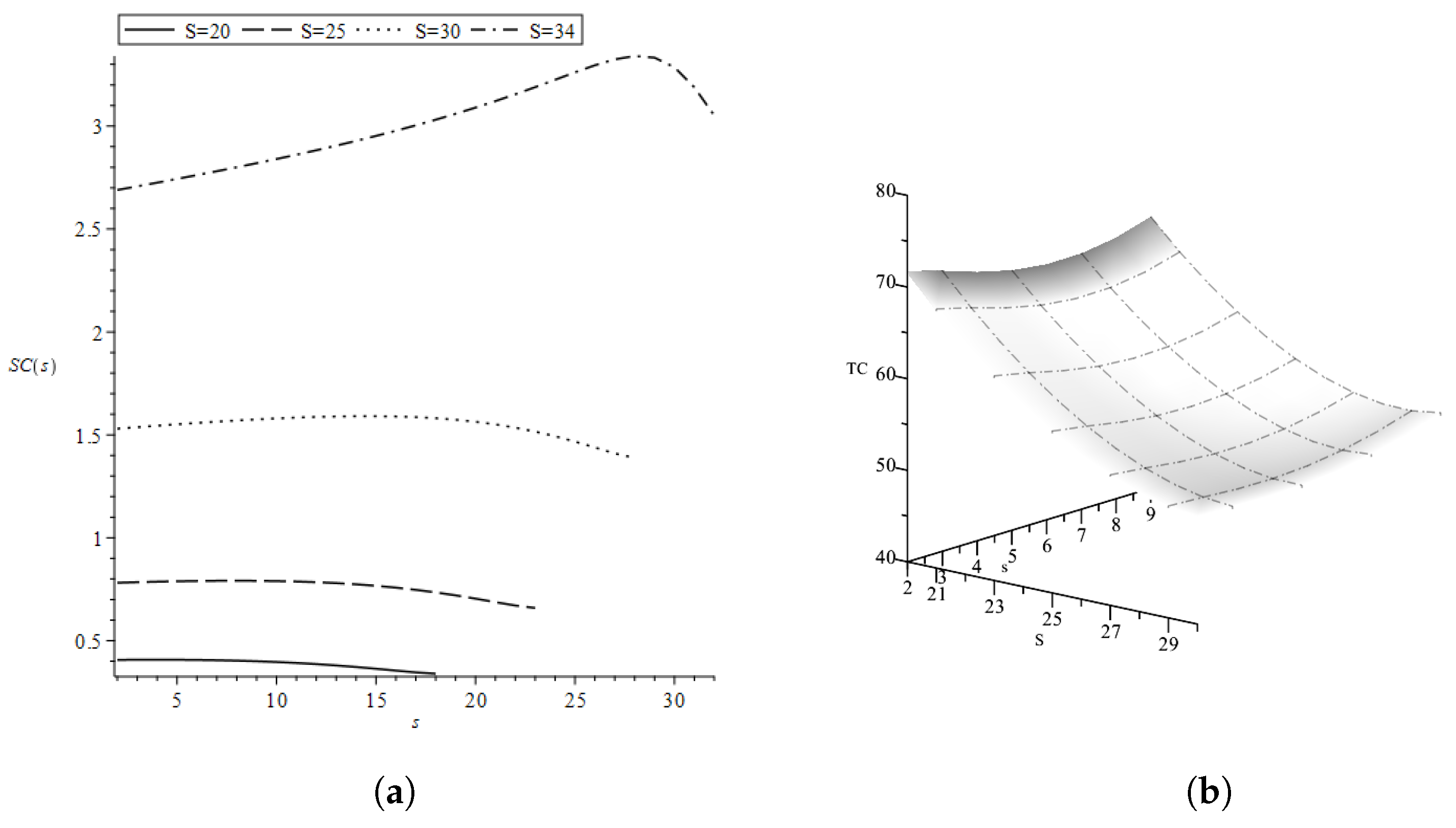
• The impact of s. Clearly, increasing s shortens the cycle length-resulting in early ordering times, and intensifies the impact of $\beta ;$ thus, the changes in $EC,OC,LC,$ and $DC$ are as expected. By contrast, the change in $SC$ is not straightforward. Figure 4a curves $SC$ as a function of $s,$ for $S=\{20,25,30,34\}$ (recall that $s<S$ and $M=35$). We see that $SC$ increases and then decreases, and these changes become more dramatic with S. At first, increasing s increases the stock, level M is hit more frequently and, thus, $SC$ increases. However, as s approaches S, the ordering time and the cycle length are significantly shortened and thus $SC$ decreases.

To summarize, while the impact of S and s on $OC$ and $LC$ is as expected, their impact on $SC$ and $DC$ is not straightforward and difficult to predict. To illustrate the overall impact, Figure 4b displays the expected discounted total cost per time unit $TC(M=35,S,s)$ as a function of S and s. We see that $TC(M=35,S,s)$ is jointly convex in S and $s;$ we note that this appears in all our examples (other values of $M,S,$ and $s$, which are not reported here, also exhibit a similar behavior). Thus, we assume that the cost is convex in $S,s$ for a fixed M. Assuming convexity enables us to numerically obtain the optimal thresholds $S^{*}$ and $s^{*}$ quicker by using a line search.

It should be noted that convexity of the total cost for base-stock policy is a common supposition, and it has been proven by several researchers for both periodic and continuous review contexts, however, for simpler models and under restricted assumption [51]. Although we cannot give a formal proof of this, we give the following intuitive explanation. Table 1 shows that the cost components are influenced in a different fashion with S and $s.$ For example, increasing S reduces the number of orders and decreases $OC$; it also reduces the penalty cost, $LC$. However, at the same time, increasing S increases $SC$ and the cycle length, and minimizes the impact of $\beta$. This trade-off between potential savings is due to fewer orders and timing on the one side, and more transferred items from the other side yields convexity.

Example 2. 

Sensitivity analysis of the optimal thresholds and cost.Here, we investigate the impact of the different parameters on the optimal thresholds and cost; we start with a balanced system.Following Example 1, we let $E\left(\xi \right)=0$ (the specific values are given in (31) and (32)), $\beta =0.075$, $\mu =0.1$, ${{\rm Y}}^{+}=50,$ and $M=35.$ We vary γ in $\{5,$ $10\},$ ${{\rm Y}}^{-}\in \{50,$ $150,\},$ $\varphi \in \{5,$ $25,$ $50,$ $100\},$ and $\nu \in \{0.5,$ $5,$ $15,$ $25,$ $100\}.$ 

Table 2. $S^{*}{,s}^{*},{TC}^{*}(M=35,S^{*}{,s}^{*})$ for ${{\rm Y}}^{-}\in \{50,150\}$, $\gamma \in \{5,10\},$ $\varphi \in \{5,25,50,100\},$ and $\nu \in \{0.5,5,15,25,100\}$.

S*, s* TC*	$\mathit{\varphi }$∖$\mathit{\nu }$	0.5	5	15	25	100
¡−= 50 $\mathit{\gamma }$= 5	5	20, 2 27.133	24, 2 29.457	19, 2 38.748	17, 2 44.792	11, 2 69.150
	25	30, 2 30.153	26, 2 40.540	21, 4 53.402	19, 4 61.845	13, 4 96.876
	50	30, 7 37.363	26, 8 48.063	23, 8 62.386	21, 8 72.243	15, 8 114.098
	100	30, 11 44.696	27, 11 55.907	23, 8 62.386	22, 11 83.298	17, 11 133.019
¡−= 50 $\mathit{\gamma }$= 10	5	20, 2 38.039	24, 2 39.811	19, 2 49.818	17, 2 56.186	11, 2 81.156
	25	30, 2 40.785	26, 2 50.760	22, 2 64.027	20, 2 72.961	13, 2 108.709
	50	30, 4 51.595	27, 5 62.358	23, 6 77.256	21, 6 87.626	15, 7 130.449
	100	30, 9 62.397	27, 9 73.001	24, 10 89.145	22, 10 100.755	17, 10 151.083
¡−= 150 $\mathit{\gamma }$= 5	5	29, 2 21.328	24, 2 29.542	19, 2 39.043	17, 2 45.280	11, 2 71.492
	25	31, 2 30.170	26, 2 40.592	21, 4 53.706	19, 4 62.347	14, 2 98.084
	50	30, 7 37.430	26, 8 48.315	23, 8 62.921	21, 8 73.131	16, 7 117.311
	100	30, 10 44.878	27, 11 56.341	24, 11 72.911	22, 11 84.850	17, 10 137.497
¡−= 150 $\mathit{\gamma }$= 10	5	28, 2 1.728	24, 2 39.896	20, 2 50.062	17, 2 56.918	11, 2 83.498
	25	30, 2 40.812	26, 2 50.811	22, 2 64.167	20, 2 73.190	13, 5 115.468
	50	30, 4 51.640	27, 5 62.446	23, 6 77.569	21, 6 88.403	15, 6 133.090
	100	30, 8 62.871	27, 9 73.255	24, 10 89.856	22, 10 101.937	17, 9 155.096

summarizes the optimal $(S^{*},s^{*})$ and the corresponding total cost $T{C}^{*}=TC(M=35,S^{*},s^{*})$.

Table 2 shows that increasing the lost cost $\varphi$ increases $S^{*}$ and $s^{*}$ (to avoid shortage); increasing $\gamma$ decreases $s^{*},$ probably to delaying the order time and, consequently, the refilling time. Additionally, $S^{*}$ is increasing in ${{\rm Y}}^{-}$ when $\nu$ and $\varphi$ are low in order to reduce the number of cancellations. We further see that, usually, increasing $\nu$ increases $s^{*}$ and thus shortens the until ordering. However, Table 2 shows few exceptions particularly when ${{\rm Y}}^{-}$ is high (${{\rm Y}}^{-}=150$); here, the distributor’s service cost cost is very high and, thus, both $S^{*}$ and $s^{*}$ are kept low to reduce the number of cancellations. Additional numerical results (that are not reported here) further show that increasing ${{\rm Y}}^{+}$ increases $S^{*}$ and decreases $s^{*}$; thereby, $S^{*}-s^{*}$ increases and the number of orders decreases.

Table 3. The impact of increasing costs on $S^{*}$ and $s^{*}$.

	The Cost ↑
$\genfrac{}{}{0.0pt}{}{\mathrm{The}\mathrm{Effect}\mathrm{on}}{}$	$\genfrac{}{}{0.0pt}{}{\mathrm{Service}\mathrm{Cost}{{\rm Y}}^{-}}{}$	$\genfrac{}{}{0.0pt}{}{\mathrm{Unit}\mathrm{Cost}\gamma }{}$	$\genfrac{}{}{0.0pt}{}{\mathrm{Loss}\mathrm{Cost}\varphi }{}$	$\genfrac{}{}{0.0pt}{}{\mathrm{Transfer}\mathrm{Cost}\nu }{}$	$\genfrac{}{}{0.0pt}{}{\mathrm{Ordering}\mathrm{Cost}{{\rm Y}}^{+}}{}$
$S^{*}$	↑	★	↑	↓	↑
$s^{*}$	★	↓	↑	★	↓

summarizes the changes in $S^{*}$ and $s^{*}$ when the costs are increasing; here, too, the star “★” stands for non-monotonic behavior.

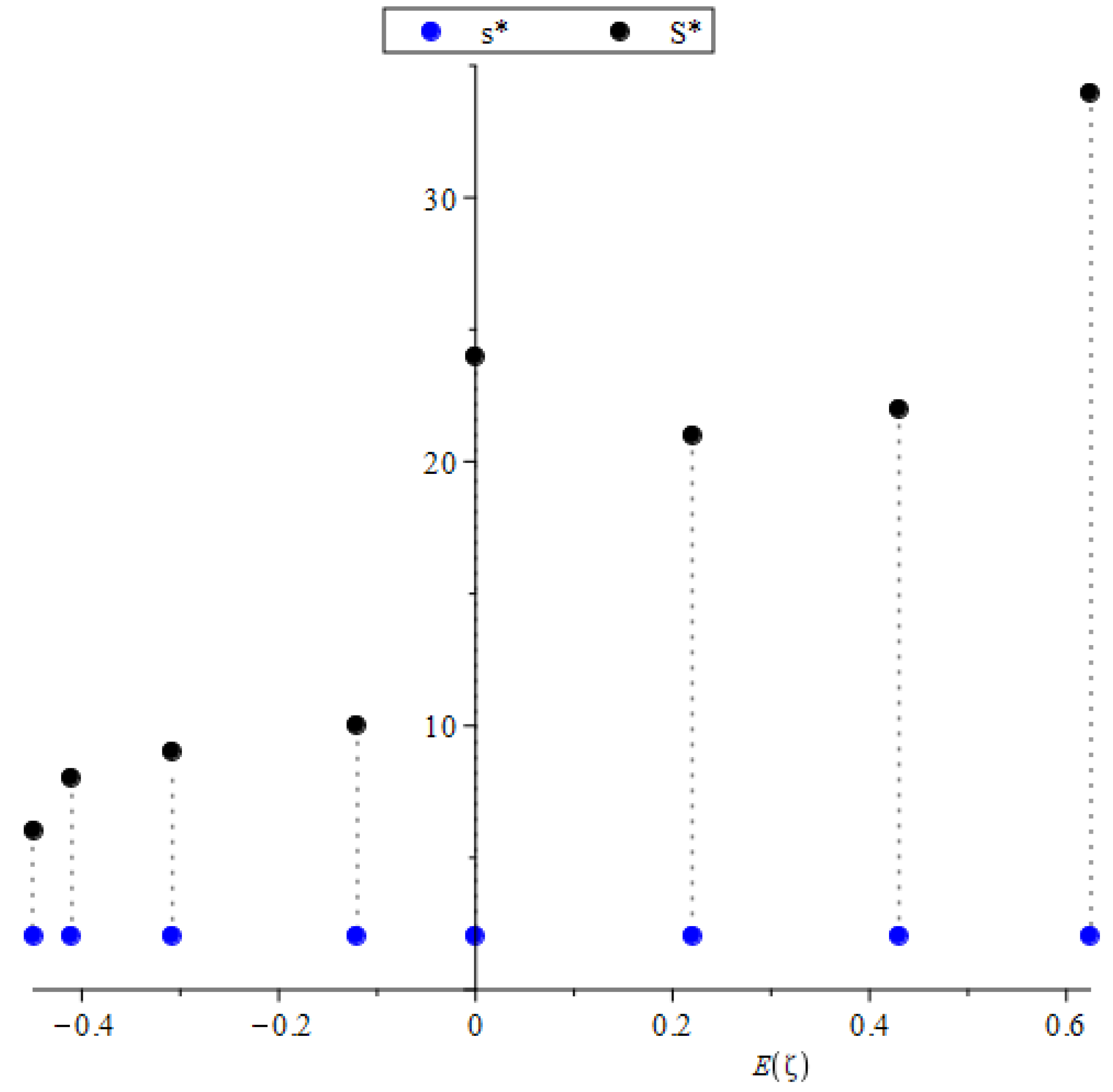
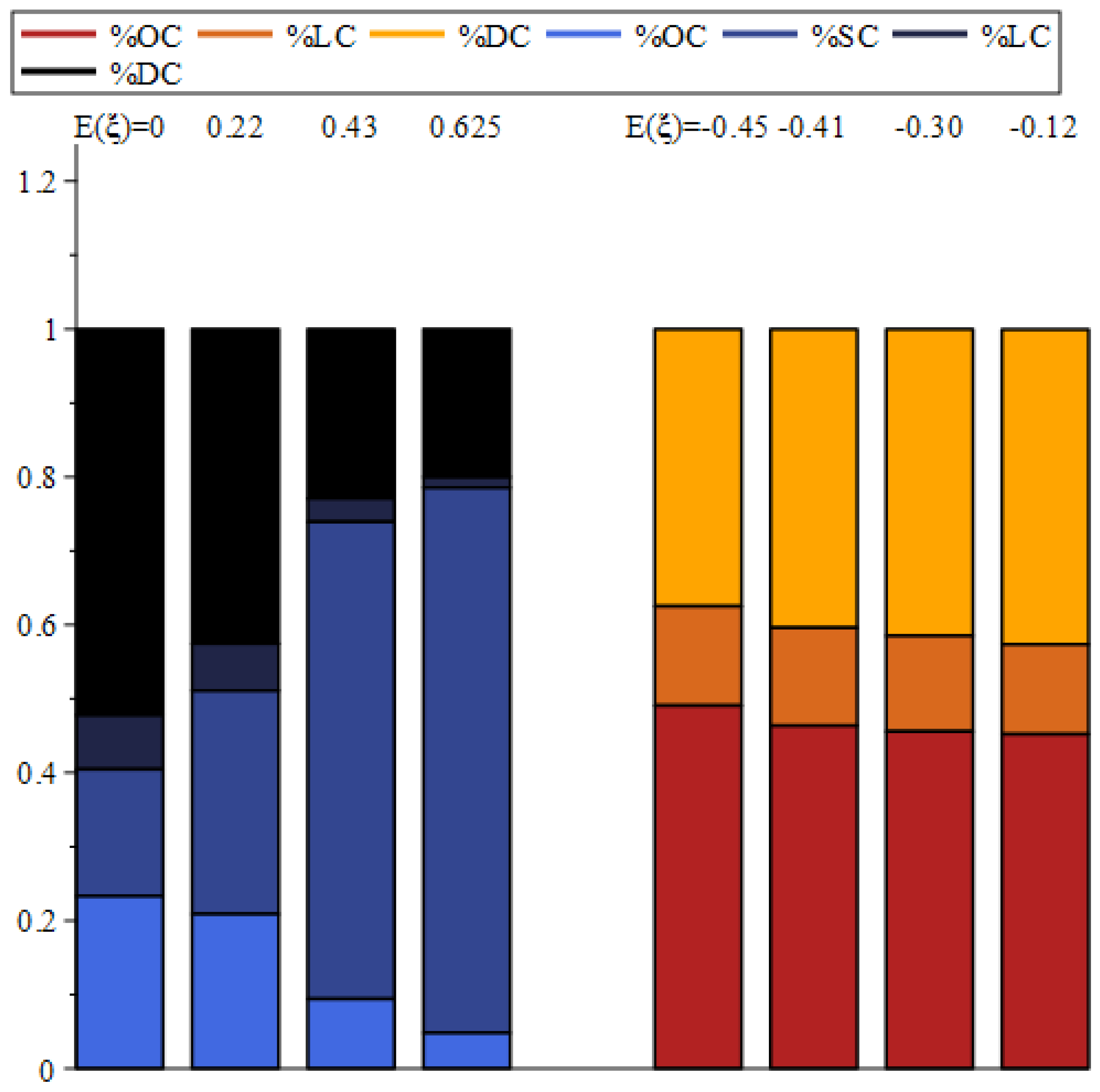
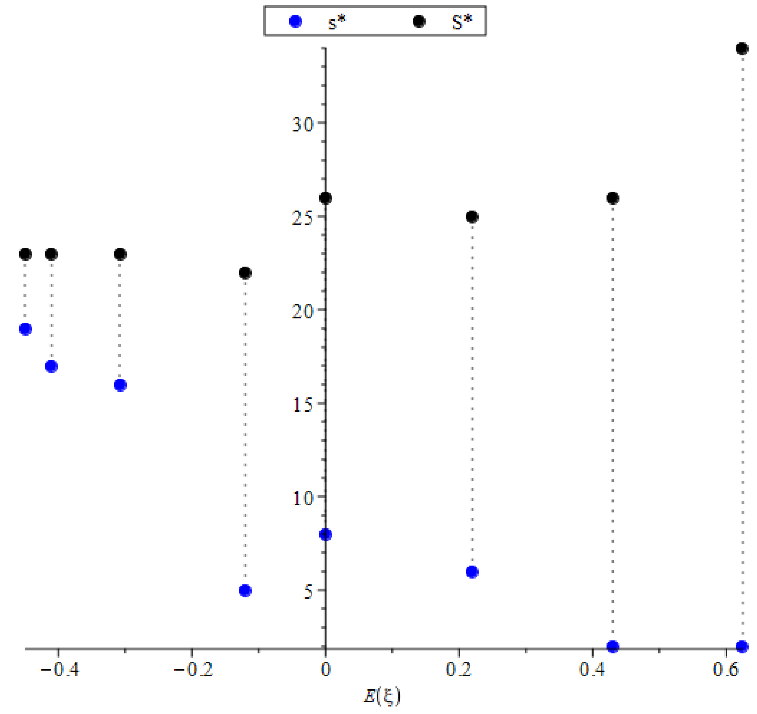
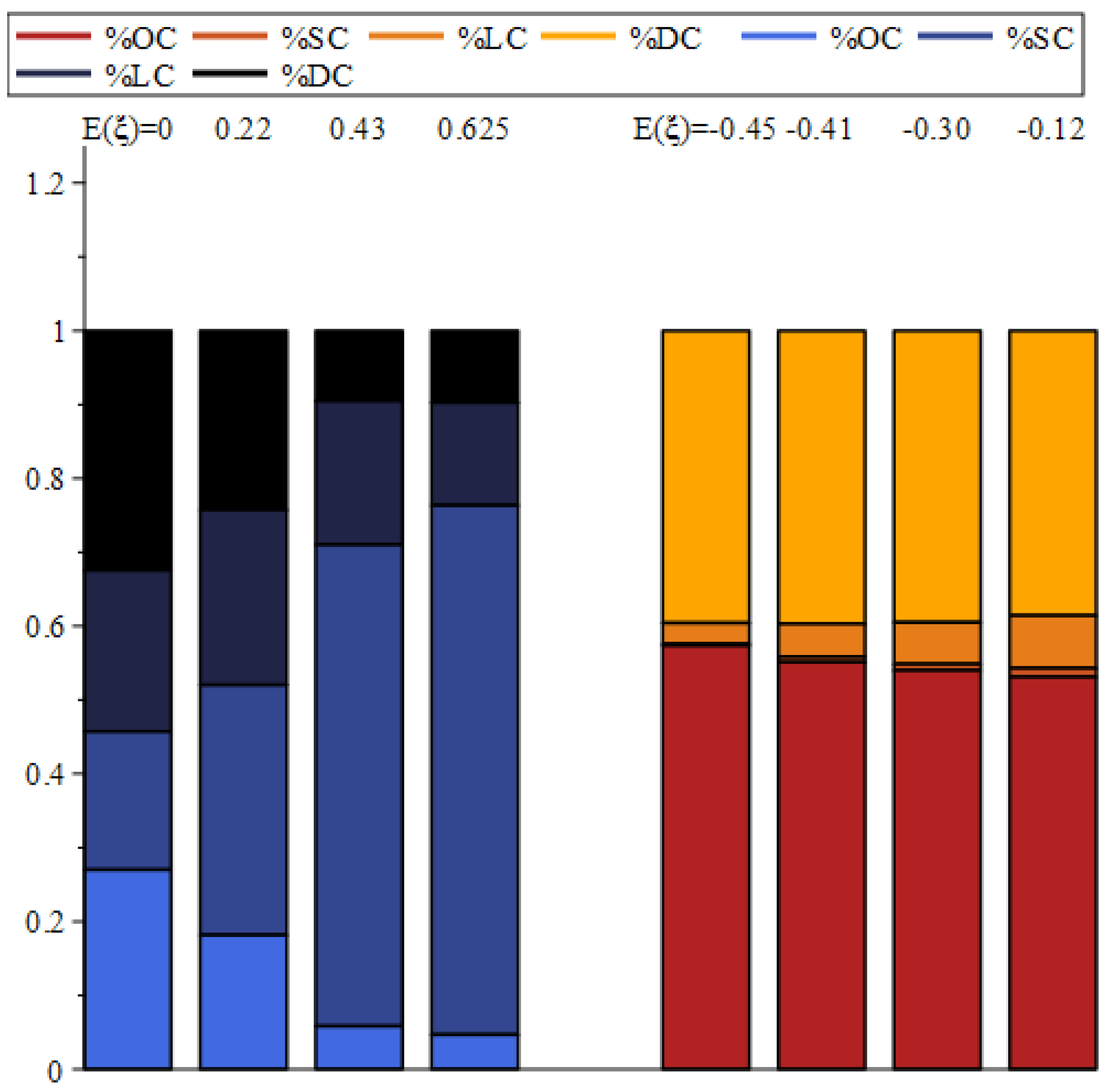
Our next goal is to study the effect of inflows and outflows (average demand and return) on the optimal thresholds $S^{*}$ and $s^{*}$. To do so, we vary $E\left(\xi \right)$ in $\{-0.45,$ $-0.41,$ $-0.308,$ $-0.24,$ $-0.12,$ $0,$ $0.22,$ $0.43,0.625\}$ by changing $c_1$ and $T^{(2+)}$ and fixing $c_2=-1.5,{\lambda }_1=0.2$ and ${\lambda }_2=0.161$ (the specific pairs $\left(c_1,E\left(U^{(2+)}\right)\right)$ corresponding to these values are $(0.025,2.5),$ $(0.03,3),$ $(0.5,1),$ $(0.2,3),$ $(0.5,3),$ $(0.5,5),$ $(0.85,5),$ $(1,7)$, and $(1.5,5),$ respectively). Recall that, when $E\left(\xi \right)<0,$ demands arrive more frequently on average, and when $E\left(\xi \right)>0,$ returns arrive more frequently (note that the results for $E\left(\xi \right)=0$ are given in Table 2). We set ${{\rm Y}}^{+}=50,$ ${{\rm Y}}^{-}=150,$ and $\nu =5,$ and focus on two scenarios: (1) $\gamma =10$ and $\varphi =5$, and (2) $\gamma =5$ and $\varphi =50.$ Scenario 1 highlights the high cost of refilling; Scenario 2 highlights the high penalty cost of a shortage. Regarding Scenario 1, Figure 5 plots the pairs $(S^{*},s^{*})$ (black and blue points, respectively) corresponding to $E\left(\xi \right),$ and Figure 6 shows the percentage of the cost components $\%OC,$ $\%LC,\%SC,$ and $\%DC$ of $T{C}^{*}.$ The blue-black scale depicts for cases where $E\left(\xi \right)\ge 0$, and the red-orange scale depicts cases where $E\left(\xi \right)<0;$ when $E\left(\xi \right)\le 0,$ the transfer cost percentage $\%SC$ becomes negligible and thus is omitted. Similarly, Figure 7 and Figure 8 plot $(S^{*},s^{*})$ and the cost percentages associated with Scenario 2, respectively. (Here, although $\%SC$ is low, it is reported).

Figure 5, Figure 6, Figure 7 and Figure 8 show that:

The levels$s^{*}$and$S^{*}.$ When the loss cost is low (i.e., Scenario 1), the level $s^{*}$ is kept low; when the loss cost is high (i.e., Scenario 2), level $s^{*}$ is significantly higher and is decreasing in $E\left(\xi \right).$ Consequently, it interesting to see that, despite the high loss cost, when $E\left(\xi \right)>0,$ $s^{*}$ is set low, probably due to the more frequent returns that reduce the number of shortages (see Figure 7). When $E\left(\xi \right)>0,$ Figure 5 and Figure 7 show similar values of $S^{*}$; we further see that $S^{*}$ is increasing in $E\left(\xi \right)$. By contrast, when $E\left(\xi \right)<0$, we see significantly higher values of $S^{*}$ under Scenario 2. Here, when demands become more frequent, the impact of the high penalty cost dominates in increasing $S^{*}$. Nevertheless, the difference ($S^{*}$–$s^{*}$) is increasing in $E\left(\xi \right)$ under both scenarios, meaning that as demands become more frequent, the optimal policy is to call the distributor more frequently and for smaller quantities.

The cost components. Our results show that, as expected, when demands become more frequent ($E\left(\xi \right)<0$) and $S^{*}$ is low, the cost percentage of $SC$ is negligible; this holds even when $S^{*}$ is set higher due to a high penalty cost (Figure 8 showing that $SC$ becomes a more significant but still meager component of the cost, less than 2%). Surprisingly, when $E\left(\xi \right)<0,$ the cost percentages remain generally similar in $E\left(\xi \right)$ under both scenarios. This can be explained by the relatively small changes in $S^{*}$. By contrast, when returns arrive more frequently, $E\left(\xi \right)>0$, we see significant changes in the cost percentages as a function of $E\left(\xi \right).$ Figure 6 and Figure 8 highlight the interplay between $\%DC$ and $\%LC.$ The percentage of the distributor’s service cost $\%DC$ is significantly higher under Scenario 1 (which is directly impacted by $\gamma$); by contrast, under Scenario 2, the loss cost $\%LC$ forms the main component of the cost. Under both scenarios, when more returns arrive, $SC$ $\left(OC\right)$ becomes the more (less) dominant component of the cost. Moreover, comparing Figure 6 and Figure 8 implies that, when $E\left(\xi \right)\ge 0,$ we have $\%S{C}_{\left\{Scenario1\right\}}\approx \%S{C}_{\left\{Scenario2\right\}}$ and $\%O{C}_{\left\{Scenario1\right\}}\approx \%O{C}_{\left\{Scenario2\right\}}.$ For example, we have $\%S{C}_{\left\{Scenario1\right\}}=\{0.17,$ $0.30,$ $0.64,$ $0.73\},$ and $\%S{C}_{\left\{Scenario2\right\}}=\{0.18,$ $0.33,$ $0.65,$ $0.71\}$ corresponding to $E\left(\xi \right)=\{0,$ $0.22,$ $0.43,$ $0.625\}$. When $E\left(\xi \right)<0,$ we have $\%D{C}_{\left\{Scenario1\right\}}\approx \%D{C}_{\left\{Scenario2\right\}}$; here, we obtain $\%D{C}_{\left\{Scenario1\right\}}=\{0.37,0.40,0.41,0.42\},$ and $\%D{C}_{\left\{Scenario2\right\}}=\{0.40,$ $0.40,$ $0.40,$ $0.38\}$ corresponding to $E\left(\xi \right)=\{-0.45,$ $-0.41,$ $-0.30,$ $-0.12\}$. These observations emphasize the company’s policy of balancing the cost components despite the different cost values. In general, when more returns arrive, and thus more items are transferred, the optimal policy aims to keep $\%SC$ relatively constant, whereas, when more demands arrive, and thus more orders are placed, the focus is to keep $\%DC$ relatively constant.

Example 3. 

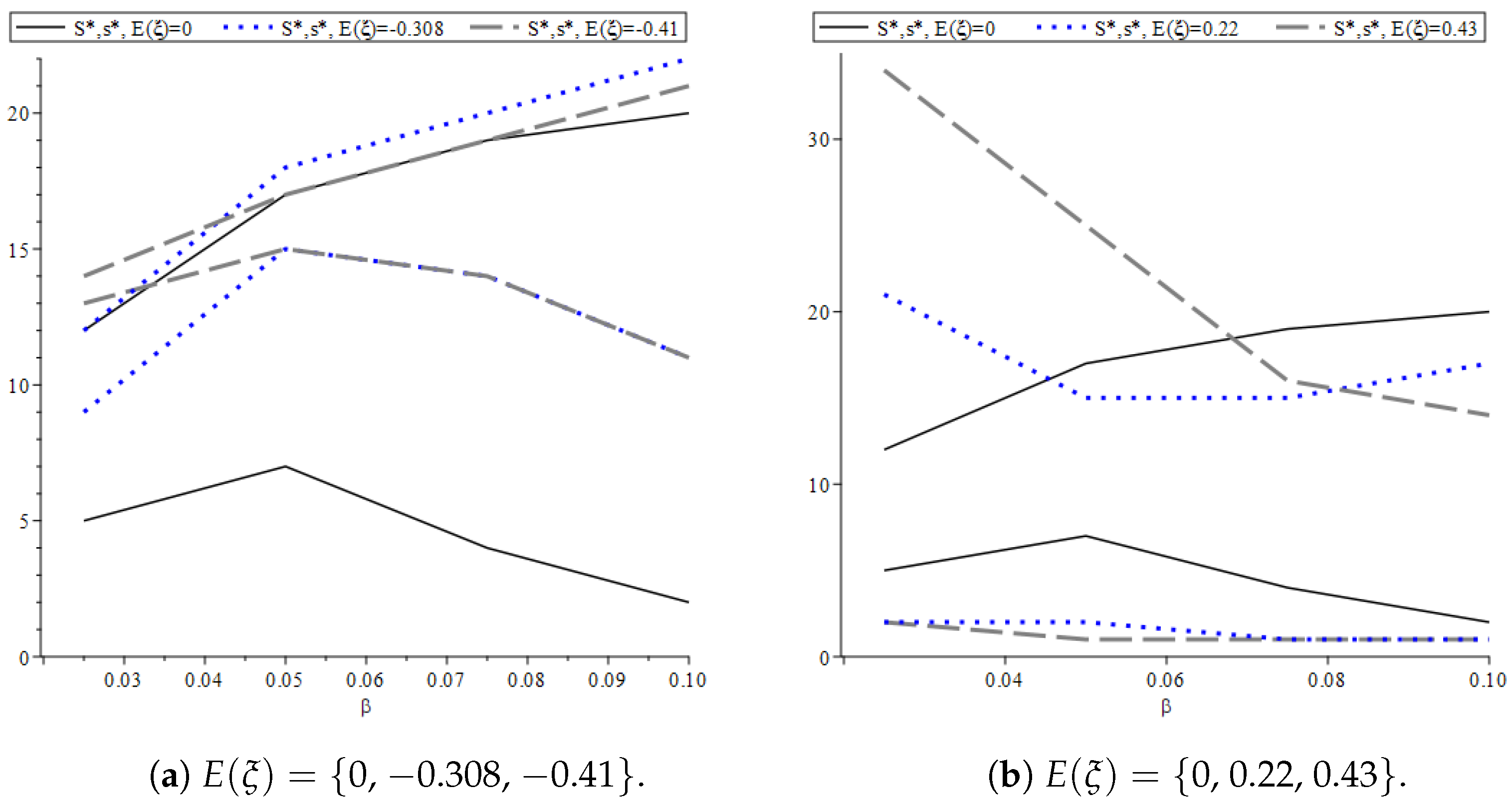
The impact of β. We next concentrate on the impact of the discounted factor β on the optimal thresholds and cost. To do so, we let ${{\rm Y}}^{-}=50,$ $\nu =25,$ $\varphi =25,$ $\gamma =5,$ $\mu =0.1,$ ${{\rm Y}}^{+}\in \{15,25,50,100\},$ and vary β in $\{0.025,0.05,0.075,0.1\}.$ 

Table 4. ${(S}^{*}{,s}^{*}),TC({M=35,S}^{*}{,s}^{*})$ as a function of $\beta ,E\left(\xi \right),$ and ${{\rm Y}}^{+}$.

S*, s* TC*		$\mathit{\beta }$
E ($\mathbf{\xi }$) = 0		0.025	0.05	0.075	0.1
¡+	15	13, 8 241.121	16, 9 92.529	17, 8 48.974	19, 5 29.221
	25	12,7 263.498	16, 8 102.091	18, 6 53.278	20, 4 31.282
	50	12, 5 313.620	17, 7 122.909	19, 4 61.845	20, 2 34.708
	100	13, 5 405.342	18, 2 155.221	21, 2 73.906	21, 1 40.932
E ($\mathbf{\xi }$) = −0.308		0.025	0.05	0.075	0.1	E ($\mathbf{\xi }$) = 0.22		0.025	0.05	0.075	0.1
¡+	15	14, 11 189.954	18, 16 98.580	20, 16 56.465	21, 14 35.679	¡+	15	15, 2 1193	13, 2 233.797	14, 5 83.106	15, 4 40.079
	25	13, 10 217.648	18, 15 117.955	21, 18 70.431	21, 13 42.855		25	21, 2 1145	14, 2 240.001	14, 2 86.883	16, 1 41.923
	50	12, 9 284.880	18, 15 165.584	20,14 97.471	22, 11 59.143		50	21, 2 1188	15, 2 254.774	15, 1 94.634	17, 1 46.180
	100	12, 9 418.205	16,13 259.948	19, 12 153.258	23, 8 87.600		100	21, 2 1274	17, 2 281.976	17, 1 108.364	18, 1 53.676
E ($\mathbf{\xi }$) = −0.41		0.025	0.05	0.075	0.1	E ($\mathbf{\xi }$) = 0.43		0.025	0.05	0.075	0.1
¡+	15	16, 15 190.886	18, 16 104.637	20, 16 60.542	20, 14 38.376	¡+	15	34, 2 959.741	25, 2 417.673	15, 1 172.134	13, 1 76.027
	25	16, 15 223.120	18, 16 125.17	19, 15 73.465	21, 14 46.47		25	34, 2 963.969	25, 2 419.423	15, 1 174.239	13, 1 77.896
	50	14, 13 302.48	17, 15 176.372	19, 14 105.381	21, 11 64.951		50	34, 2 974.540	25, 1 423.796	16, 1 179.223	14, 1 82.263
	100	12, 11 454.858	16, 14 277.973	19, 13 167.416	23, 9 97.662		100	34, 2 995.681	26, 1 432.543	17, 1 197.933	15, 1 89.658

presents the optimal policy and cost; it includes five subtables that differ in their $E\left(\xi \right).$ The top subtable corresponds to $E\left(\xi \right)=0$, the two left-hand subtables correspond to the negative $E\left(\xi \right)=\{-0.308,$ $-0.41\},$ and the two right-hand subtables correspond to the positive $E\left(\xi \right)=\{0.22,$ $0.43\}.$ Each subtable presents the levels $(S^{*},s^{*})$ and the cost $TC(S^{*},s^{*},M=35)$ for different values of β; the entry $E\left(\xi \right)=0,$ $\beta =0.075,$ ${{\rm Y}}^{+}=50$ is also given in Table 2. Figure 9a curves $S^{*}$ and $s^{*}$ as a function of $\beta ,$ for $E\left(\xi \right)=\{0,$ $-0.308,$ $-0.41\}$ (the black, blue, and gray curves, respectively); similarly, Figure 9b curves $S^{*}$ and $s^{*}$ for $E\left(\xi \right)=\{0,$ $0.22,$ $0.43\}$ (the black, blue, and gray curves, respectively). (Here, we take ${{\rm Y}}^{+}=50.$) Note that both figures contain the case $E\left(\xi \right)=0,$ indicated by the black curves.

From Table 4 and Figure 9, we derive the following conclusions:

• As expected, the cost $T{C}^{*}$ is decreasing in $\beta$ and is increasing in ${{\rm Y}}^{+}.$ We further see that, while increasing ${{\rm Y}}^{+}$ decreases $s^{*}$ (in accordance with Table 3), the changes of $S^{*}$ in ${{\rm Y}}^{+}$ are not monotone and are impacted also by $\beta$ and $E\left(\xi \right)$ (in fact, $S^{*}$ varies slightly in ${{\rm Y}}^{+}$).
• When $E\left(\xi \right)\le 0,$ the level $S^{*}$ is increasing in $\beta ,$ while $s^{*}$ seems to be concave. Hence, increasing $\beta$ increases the difference $S^{*}$–$s^{*}$ (noted that a balanced system with $E\left(\xi \right)=0$ is also included here; see Table 3). When the value of $\beta$ is high, then, despite the fact that demands become more frequent, it is economically profitable for the company to postpone ordering and thereby increase the quantity of refilling.
• By contrast, when $E\left(\xi \right)>0,$ we see that $S^{*}$ is convex in $\beta ,$ and $s^{*}$ is decreasing. Here, the difference $S^{*}$–$s^{*}$ is convex in $\beta$. In general, as more returns arrive, and for low values of $\beta ,$ the company’s main motivation is to reduce the transfer cost by decreasing $S^{*},s^{*}$ and reducing $S^{*}$–$s^{*}.$ However, as $\beta$ increases, we see a slight increase in $S^{*}$ (see Figure 9b, particularly the dotted blue curve when $\beta \ge 0.08$). The main implication is to postpone the distributor in order to achieve a full utilization of the discount factor.

Summarizing, we see that the discount factor, and the interplay between returns and demands, have a crucial impact on determining the optimal policy and obtaining a decisive economic advantage.

7. Conclusions

This paper studies an inventory control problem with two types of storage facilities that differ in purpose and capacity. We consider continuous and batch-type bilateral changes in the inventory level, where both types of changes are governed by the underlying Markov chain. Applying first passage time results, we build a relatively easy set of equations to derive the cost components under the discounted criterion and lost sales assumption. In doing so, we provide managers with a useful and efficient tool to derive, numerically, the optimal parameters. We show that the limited capacity yields lower thresholds, and as demands become more frequent, it is worthwhile to order more frequently and in smaller quantities. We further show that the timing has a significant impact on the optimal policy; for high values of $\beta$, it is worth considering postponing the distributor even at the risk of causing more shortage events.

For future research, it will be interesting to consider the case where each refilling order proceeds sequentially for a few stages, each of which has an independent exponential distributed time. Thus, the total time it would take to handle the order could be expressed by the phase-type distribution rather than by an exponential one. In particular, nowadays, when collaborative inventories and outsourcing services are widespread, it is practical to assume that each order has to go through several procedures, e.g., due to miscellaneous certificates, multiple managers, or different hierarchical ranks. Our approach in this study appears to be simple and easy to implement; thus, we believe that it can be applied as a powerful tool to address other inventory policies. For example, upon adding the option of backordering up to some fixed level, thereafter the unsatisfied demand will be lost. Another well-known policy is the $(Q,r)$ policy, where a fixed order of size Q is placed whenever the on-hand stock level drops to or below level r. Finally, a combination of the above-mentioned policies can also be considered. Each of the discussed policy is worth studying and hence is left for future investigation.

References

- Kuraie, V.C.; Padiyar, S.S.; Bhagat, N.; Singh, S.R.; Katariya, C. Imperfect production process in an integrated inventory system having multivariable demand with limited storage capacity. Des. Eng. 2021, 2021, 1505–1527. [Google Scholar]
- Asmussen, S. Applied Probability and Queues, 2nd ed.; Springer: New York, NY, USA, 2003. [Google Scholar]
- Rodríguez-García, M.C.; Gutiérrez-Puertas, L.; Granados-Gámez, G.; Aguilera-Manrique, G.; Mxaxrquez-Hernxaxndez, V.V. The connection of the clinical learning environment and supervision of nursing students with student satisfaction and future intention to work in clinical placement hospitals. J. Clin. Nurs. 2021, 30, 986–994. [Google Scholar] [CrossRef] [PubMed]
- Barron, Y.; Dreyfuss, M. A triple (S,s,ℓ) -thresholds base-stock policy subject to uncertainty environment, returns and order cancellations. Comput. Oper. Res. 2021, 134, 105320. [Google Scholar] [CrossRef]
- Perera, S.; Janakiraman, G.; Niu, S.C. Optimality of (s,S) inventory policies under renewal demand and general cost structures. Prod. Oper. Manag. 2018, 27, 368–383. [Google Scholar] [CrossRef]
- Benkherouf, L.; Bensoussan, A. Optimality of an (s,S) policy with compound Poisson and diffusion demands: A quasi-variational inequalities approach. SIAM J. Control Optim. 2009, 48, 756–762. [Google Scholar] [CrossRef]
- Pérez, J.L.; Yamazaki, K.; Bensoussan, A. Optimal periodic replenishment policies for spectrally positive Lévy demand processes. SIAM J. Control Optim. 2020, 58, 3428–3456. [Google Scholar] [CrossRef]
- Yamazaki, K. Inventory control for spectrally positive Lèvy demand processes. Math. Oper. Res. 2017, 42, 212–237. [Google Scholar] [CrossRef]
- Yao, D.; Chao, X.; Wu, J. Optimal control policy for a brownian inventory system with concave ordering cost. J. Appl. Probab. 2015, 52, 909–925. [Google Scholar] [CrossRef]
- Dbouk, W.; Tarhini, H.; Nasr, W. Re-ordering policies for inventory systems with a fluctuating economic environment—Using economic descriptors to model the demand process. J. Oper. Res. Soc. 2022, 1–13. [Google Scholar] [CrossRef]
- Germain, R.; Claycomb, C.; Dröge, C. Supply chain variability, organizational structure, and performance: The moderating effect of demand unpredictability. J. Oper. Manag. 2008, 26, 557–570. [Google Scholar] [CrossRef]
- Barron, Y. A state-dependent perishability (s,S) inventory model with random batch demands. Ann. Oper. Res. 2019, 280, 65–98. [Google Scholar] [CrossRef]
- Barron, Y. The continuous (S,s,Se) inventory model with dual sourcing and emergency orders. Eur. J. Oper. Res. 2022, 301, 18–38. [Google Scholar] [CrossRef]
- Lu, Y. Estimation of average backorders for an assemble-to-order system with random batch demands through extreme statistics. Nav. Res. Logist. 2007, 54, 33–45. [Google Scholar] [CrossRef]
- Feng, L.; Chan, Y.L. Joint pricing and production decisions for new products with learning curve effects under upstream and down stream trade credits. Eur. J. Oper. Res. 2019, 272, 905–913. [Google Scholar] [CrossRef]
- Hu, K.; Acimovic, J.; Erize, F.; Thomas, D.J.; Van Mieghem, J.A. Forecasting new product life cycle curves: Practical approach and empirical analysis: Finalist-2017 M&SOM practice-based research competition. Manuf. Serv. Oper. Manag. 2018, 21, 66–85. [Google Scholar]
- Avci, H.; Gokbayrak, K.; Nadar, E. Structural results for average-cost inventory models with Markov-modulated demand and partial information. Prod. Oper. Manag. 2020, 29, 156–173. [Google Scholar] [CrossRef]
- Barron, Y. An order-revenue inventory model with returns and sudden obsolescence. Oper. Res. Lett. 2018, 46, 88–92. [Google Scholar] [CrossRef]
- Ozkan, C.; Karaesmen, F.; Ozekici, S. Structural properties of Markov modulated revenue management problems. Eur. J. Oper. Res. 2013, 225, 324–331. [Google Scholar] [CrossRef]
- Ishfaq, R.; Raja, U.; Rao, S. Seller-induced scarcity and price-leadership. Int. J. Logist. Manag. 2016, 27, 552–569. [Google Scholar] [CrossRef]
- Rudolph, S. E-commerce product return statistics and trends. Bus. Community 2016. [Google Scholar]
- Chen, L.; Song, J.S.; Zhang, Y. Serial inventory systems with Markov-modulated demand: Derivative bounds, asymptotic analysis, and insights. Oper. Res. 2017, 65, 1231–1249. [Google Scholar] [CrossRef]
- Nasr, W.W. Inventory systems with stochastic and batch demand: Computational approaches. Ann. Oper. Res. 2022, 309, 163–187. [Google Scholar] [CrossRef]
- Perera, S.C.; Sethi, S. A survey of stochastic inventory models with fixed costs: Optimality of (s,S) and (s,S)-type policies. Prod. Oper. Manag. 2022, 32, 154–169. [Google Scholar] [CrossRef]
- Presman, E.; Sethi, S.P. Inventory models with continuous and Poisson demands and discounted and average costs. Prod. Oper. Manag. 2006, 15, 279–293. [Google Scholar] [CrossRef]
- Ahn, S. Time-dependent and stationary analyses of two-sided reflected Markov-modulated Brownian motion with bilateral ph-type jumps. J. Korean Stat. Soc. 2017, 46, 45–69. [Google Scholar] [CrossRef]
- Breuer, L. A quintuple law for Markov additive processes with phase-type jumps. J. Appl. Probab 2010, 47, 441–458. [Google Scholar] [CrossRef]
- Dudin, A.; Dudina, O.; Dudin, S.; Samouylov, K. Analysis of single-server multi-class queue with unreliable service, batch correlated arrivals, customers impatience, and dynamical change of priorities. Mathematics 2021, 9, 1257. [Google Scholar] [CrossRef]
- Yamazaki, K. Cash management and control band policies for spectrally one-sided Lèvy processes. Recent Adv. Financ. Eng. 2016, 2014, 199–215. [Google Scholar]
- Zhang, Z. Dynamic Cash Management Models. Ph.D. Thesis, Lancaster University, Lancaster, UK, 2022. [Google Scholar]
- Yan, K. Fluid Models for Production-Inventory Systems. Ph.D. Thesis, The University of North Carolina at Chapel Hill, Chapel Hill, NC, USA, 2006. [Google Scholar]
- Kawai, Y.; Takagi, H. Fluid approximation analysis of a call center model with time-varying arrivals and after-call work. Oper. Res. Perspect. 2015, 2, 81–96. [Google Scholar] [CrossRef]
- Cao, P.; Yao, D. Dual sourcing policy for a continuous-review stochastic inventory system. IEEE Trans. Automat. Control 2019, 64, 2921–2928. [Google Scholar] [CrossRef]
- Gong, M.; Lian, Z.; Xiao, H. Inventory control policy for perishable products under a buyback contract and Brownian demands. Int. J. Prod. Econ. 2022, 251, 108522. [Google Scholar] [CrossRef]
- He, S.; Yao, D.; Zhang, H. Optimal ordering policy for inventory systems with quantity-dependent setup costs. Math. Oper. Res. 2017, 42, 979–1006. [Google Scholar] [CrossRef]
- Li, Y.; Sethi, S. Optimal Ordering Policy for Two Product Inventory Models with Fixed Ordering Costs. 2022. Available online: https://ssrn.com/abstract=4199040 (accessed on 26 December 2022).
- Anbazhagan, N.; Joshi, G.P.; Suganya, R.; Amutha, S.; Vinitha, V.; Shrestha, B. Queueing-inventory system for two commodities with optional demands of customers and MAP arrivals. Mathematics 2022, 10, 1801. [Google Scholar] [CrossRef]
- Vinitha, V.; Anbazhagan, N.; Amutha, S.; Jeganathan, K.; Shrestha, B.; Song, H.K.; Joshi, G.P.; Moon, H. Analysis of a stochastic inventory model on random environment with two classes of suppliers and impulse customers. Mathematics 2022, 10, 2235. [Google Scholar] [CrossRef]
- López, D.M.; Pérez, J.L.; Yamazaki, K. Effects of positive jumps of assets on endogenous bankruptcy and optimal capital structure: Continuous-and periodic-observation models. SIAM J. Financ. Math. 2021, 12, 1112–1149. [Google Scholar] [CrossRef]
- Noba, K.; Yamazaki, K. On stochastic control under Poisson observations: Optimality of a barrier strategy in a general Lévy model. arXiv 2022, arXiv:2210.00501. [Google Scholar]
- Bensoussan, A.; Liu, R.H.; Sethi, S.P. Optimality of an (s,S) policy with compound Poisson and diffusion demands: A quasi-variational inequalities approach. SIAM J. Control Optim. 2005, 44, 1650–1676. [Google Scholar] [CrossRef]
- Chakravarthy, S.R.; Rao, B.M. Queuing-inventory models with MAP demands and random replenishment opportunities. Mathematics 2021, 9, 1092. [Google Scholar] [CrossRef]
- Azcue, P.; Muler, N. Optimal cash management problem for compound Poisson processes with two-sided jumps. Appl. Math. Optim. 2019, 80, 331–368. [Google Scholar] [CrossRef]
- Deelstra, G.; Latouche, G.; Simon, M. On barrier option pricing by Erlangization in a regime-switching model with jumps. J. Comput. Appl. Math. 2020, 371, 112606. [Google Scholar] [CrossRef]
- Kijima, M.; Siu, C.C. On the First Passage Time under Regime-Switching with Jumps. In Inspired by Finance; Springer: Cham, Switzerland, 2014; pp. 387–410. [Google Scholar]
- Chew, A.; Mus, S.; Rohloff, P.; Barnoya, J. The Relationship between Corner Stores and the Ultra-processed Food and Beverage Industry in Guatemala: Stocking, Advertising, and Trust. J. Hunger Environ. Nutr. 2022, 1–16. [Google Scholar] [CrossRef]
- Mandi, E.; Chen, X.; Zhou, K.Z.; Zhang, C. Loose lips sink ships: The double-edged effect of distributor voice on channel relationship performance. Ind. Mark. Manag. 2022, 102, 141–152. [Google Scholar] [CrossRef]
- Sato, K.; Yagi, K.; Shimazaki, M. A stochastic inventory model for a random yield supply chain with wholesale-price and shortage penalty contracts. Asia-Pac. J. Oper. Res. 2018, 35, 1850040. [Google Scholar] [CrossRef]
- Ramaswami, V. Passage times in fluid models with application to risk processes. Methodol. Computat. Appl. Probab. 2006, 8, 497–515. [Google Scholar] [CrossRef]
- Asmussen, S.; Kella, O. A multi-dimensional martingale for Markov additive processes and its applications. Adv. Appl. Probab. 2000, 32, 376–393. [Google Scholar] [CrossRef] [Green Version]
- Bijvank, M.; Vis, I.A.F. Lost sales inventory theory: A review. Eur. J. Oper. Res. 2011, 215, 1–13. [Google Scholar] [CrossRef]
Figure 1.
The relationship between the manufacturer, distributor, customers, and warehouses.
Figure 2.
A typical sample path of and .
Figure 3.
The MMFF process for .
Figure 4.
(a) for (b) as a function of S and .
Figure 5.
corresponding to Scenario 1.
Figure 6.
The %cost components, Scenario 1.
Figure 7.
corresponding to Scenario 2.
Figure 8.
The %cost components, Scenario 2.
Figure 9.
The levels and as a function of and .