Comparative Study of Numerical Methods for Solving the Fresnel Integral in Aperiodic Diffractive Lenses

Abstract

In this work, we present a comparative analysis of different numerical methods to obtain the focusing properties of the zone plates based on Fibonacci and Cantor sequences. The Fresnel approximation was solved numerically in order to obtain the axial irradiance provided by these diffractive lenses. Two different methods were applied. The first one is based on numerical integration, specifically the Simpson integration method and the two-dimensional Gaussian quadrature. The second consisted in the implementation of the Fast Fourier Transform in both one and two dimensions. The axial irradiance of the lenses, the relative error with respect to the analytical solution, and the calculation time required by each method are analyzed and compared. From this analysis it was concluded that the Gauss method presents the best balance between accuracy and computation time. This analysis could be useful to decide the most convenient numerical method to be used for the study of more complex diffractive structures.

1. Introduction

In its simplest form, a diffractive lens also known as Zone Plate (ZP) [1] is characterized by a series of concentric annular rings, alternately transparent and opaque at the wavelength for which they have been designed. Therefore, conventional ZPs are structured periodically along the squared radial coordinate, where each pair of zones constitutes a period thus making the area of the annular zones constant. This zone configuration produces a series of convergent spherical waves by diffraction when it is illuminated by a monochromatic plane wave, hence generating a series of foci along the optical axis.

In the last decade, the study of diffractive structures has become more relevant due to their particular multifocal characteristics [1]. Diffractive elements are a widely used tool in different areas of science, such as biology, ophthalmology, and materials science, among others [2,3,4]. The continuous development of applications using diffractive lenses has shown their potential for the optimization of optical systems. This is because they add new features, such as the generation of multiple foci on the axial axis. An example of this is the implementation of an aperiodic kinoform diffractive lens in an optical tweezers system [5]. The design of new aperiodic ZP using different structures, such as Triadic Cantor Set or Fibonacci sequence [6,7], allows for finding axial irradiance distributions associated with each of them. This is why the characterization of the focusing properties of ZPs is of utmost importance in the design of these diffractive elements.

The study of the focusing properties of these aperiodic ZPs is mainly based on the Fresnel approach. This model allows to obtain the irradiance distribution along the optical axis. However, sometimes the Fresnel diffraction integral is difficult to be obtained analytically, and the implementation of numerical methods such as the Fast Fourier Transform or the Simpson and Gaussian quadrature methods are somes of the employed up to now options [8].

Numerical integration methods have a wide range of applications in medicine, electronics, fluid dynamics, optics, machinery, information, etc. [9,10,11,12]. The main interests of these numerical schemes include approximation, estimation, and computation time, and they are used in virtually every scientific field. Towards this aim, several numerical integrators have been developed [13,14,15] and various numerical integration techniques have been derived [16,17].

For the specific case of the Fresnel integrals, among the most used methods are the Riemann rule, the trapezoidal rule, the Simpson’s rule and the Gaussian quadrature [18,19,20]. Several studies comparing these methods focus on analyzing how the error of the method varies with respect to the sampling used. This error can be calculated as the absolute difference between the numerical and the analytical solution or as the root mean square error relative to experimental data [9,10,11,12].

A fast Fourier transform (FFT) is an algorithm that computes the discrete Fourier transform (DFT) of a sequence, or its inverse. Fast Fourier transforms are widely used for applications in engineering, music, science, and mathematics. Since the Fresnel integral can be written in terms of a Fourier transform, this method can be used to study the focusing properties of diffractive optical elements [21].

Each of these methods approaches the solution of the Fresnel integral in a different way, so the computation time and the error rate vary between them. According to the diffractive structure symmetry, the methods can be approached in a two-dimensional way, a one-dimensional way, or both. The characteristics of each of these methods make them suitable depending on the region of space where it is desired to obtain the irradiance properties of the lens. In this work, we perform a comparative analysis of these numerical methods to obtain the axial irradiance of fractal and Fibonacci ZPs. Computation times and relative errors are presented for each method.

2. Mathematical Model

One of the main aspects in the design and study of diffractive elements is obtaining the irradiance pattern associated with each zone plate. The focusing properties of each ZP allow to know how the incident radiation interacts with it, creating an axial distribution of irradiance determined by its geometric configuration. The theory that describes this is the so-called Fresnel diffraction integral. The propagation of a wavefront through a finite aperture or an object located at position $P(x,y,z)$, can be obtained through the evaluation of the Fresnel diffraction integral, which is usually expressed as [22],

$$U(x,y,z)=-\frac{e^{-ikz}{e}^{-\frac{ik}{2z}(x^2+y^2)}}{i\lambda z}{\int \int }_{-\infty }^{\infty }At(x_0,y_0)e^{\frac{-ik}{2z}(x_0^2+y_0^2)}{e}^{\frac{ik}{z}(x{x}_0+y{y}_0)}d{x}_{0}d{y}_0$$

(1)

where A is the amplitude of the optical field at the aperture, $t(x_0,y_0)$ is the transmittance function of the diffractive structure, $k=\frac{2\pi }{\lambda }$ is the angular wave number, $\lambda$ is the wavelength, and the integration limits correspond to the opening dimensions (see Figure 1).

This expression can be interpreted as a superposition of spherical waves in the paraxial approximation and is considered valid for the near-field region or the so-called Fresnel diffraction region. In this approximation, the distance between the lens and the focusing plane is much larger than the lens size. Thus, from Equation (1), the irradiance can be obtained as the square of the amplitude for the diffracted field. Using normalized coordinates for the pupil plane as ${\overline{x}}_0=\frac{x_0}{a}$, ${\overline{y}}_0=\frac{y_0}{a}$, the irradiance is given by,

$$I(x,y,u)=4A^2{u}^2{\left|{\int \int }_{-\infty }^{\infty }t({\overline{x}}_0,{\overline{y}}_0)e^{i2\pi u({\overline{x}}_0^2+{\overline{y}}_0^2)}{e}^{-i2\pi 2u(x{\overline{x}}_0+y{\overline{y}}_0)}d{\overline{x}}_{0}d{\overline{y}}_0\right|}^2$$

(2)

where $u=\frac{a^2}{2\lambda z}$ is the reduced axial coordinate, and a is the external radius of the lens [6].

Apart from the multiplicative factor that precedes the integral, the irradiance distribution in an observation plane u, perpendicular to the optical axis, can be defined in terms of the two-dimensional Fourier transform evaluated for the transmittance function $t({\overline{x}}_0,{\overline{y}}_0)$ multiplied by $e^{i2\pi u({\overline{x}}_0^2+{\overline{y}}_0^2)}$ [23]. If only the irradiance along the propagation axis is considered, Equation (2) becomes,

$$I\left(u\right)=4A^2{u}^2{\left|{\int \int }_{-\infty }^{\infty }t({\overline{x}}_0,{\overline{y}}_0)e^{i2\pi u({\overline{x}}_0^2+{\overline{y}}_0^2)}d{\overline{x}}_{0}d{\overline{y}}_0\right|}^2$$

(3)

Indeed, for a diffractive element with radial symmetry, Equation (3) can be simplified as [7],

$$I\left(u\right)=4{\pi }^2{u}^2{\left|\underset{0}{\overset{1}{\int }}t\left(\zeta \right)e^{-i2\pi u\zeta }d\zeta \right|}^2$$

(4)

where a coordinate transformation $\zeta ={\left(\frac{r_0}{a}\right)}^2$ is introduced, being $r_0$ the radial coordinate of the lens. It can be observed that similarly to Equation (2), the axial irradiance distribution is given by the one-dimensional Fourier transform of the transmittance function.

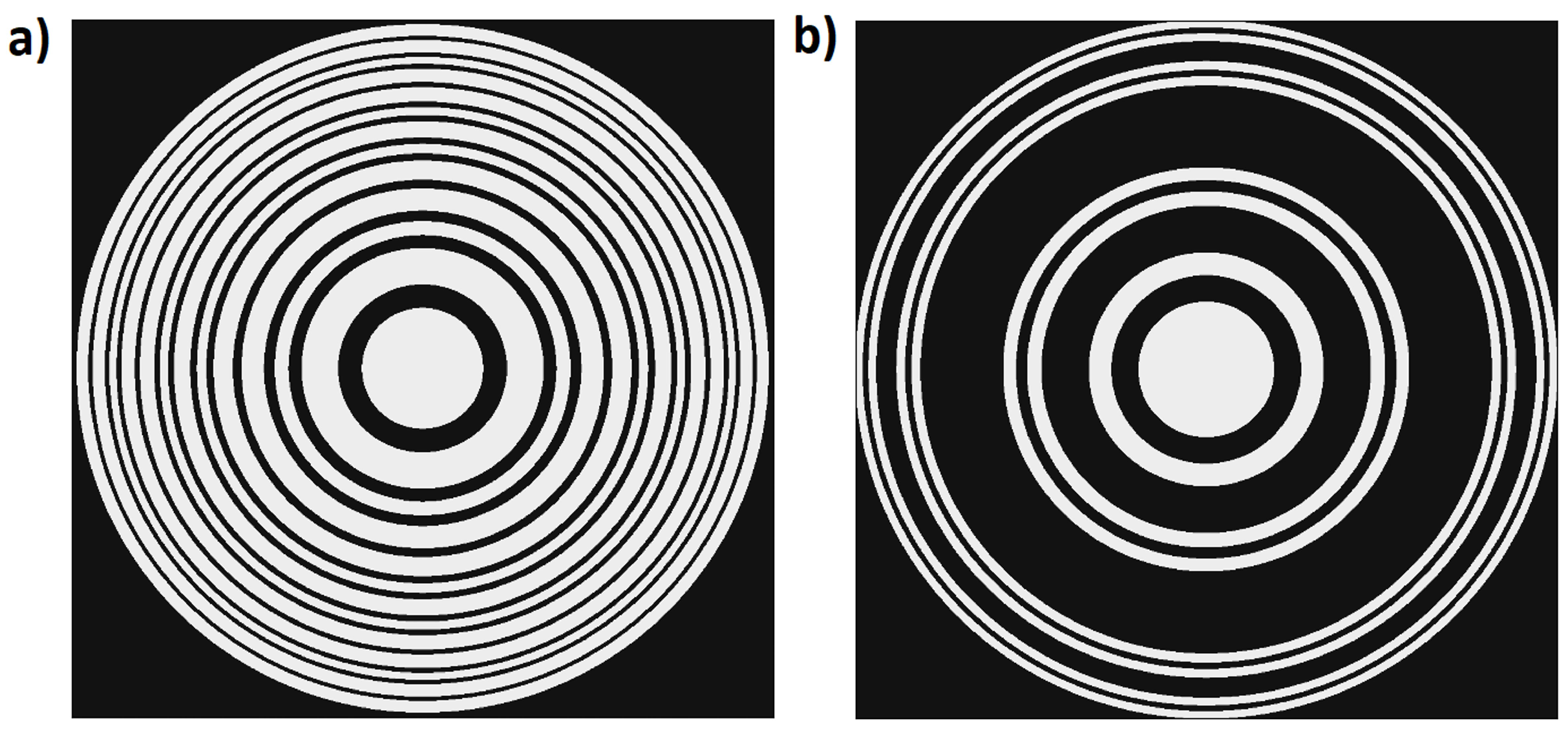
The distribution of transparent and opaque zones in a ZP can be based on aperiodic sequences, which gives rise to different irradiance distributions along the optical axis. To build these sequences, an iterative method can be applied [24]. We start from a seed element $S_0$ and the higher orders are generated using a particular set of substitution rules. Two of the most studied sequences are Fibonacci and Triadic Cantor due to their focusing properties [6,7]. For the Fibonacci sequence, the seed element is $S_0=A$ and the substitution rules are $g\left(A\right)=AB$ and $g\left(B\right)=A$. For the Triadic Cantor sequence, the seed element is $S_0=A$, and the substitution rules are $g\left(A\right)=ABA$ and $g\left(B\right)=BBB$. These sequences can be used to define the distribution of transparent and opaque zones of the ZP, where A is a transparent zone and B is an opaque one, both with the same area. Assigning one of these sequences to the variable $\zeta$ and applying symmetry of revolution around the axis, we obtain the corresponding aperiodic ZP, where $t\left(\zeta \right)=1$ in type A zones and $t\left(\zeta \right)=0$ in type B zones. In this work, we used the ZP based on the Fibonacci sequence of order $S=8$ and the ZP based on the Triadic Cantor sequence of order $S=3$, which have been represented in Figure 2.

In this article, a comparative analysis of the implementation of one-dimensional and two-dimensional numerical integration methods in the solution of the Fresnel diffraction integral is carried out. Equations (3) and (4) were solved using the Simpson numerical integration method and the 2D Gaussian quadrature, respectively. Moreover, one-dimensional and two-dimensional Fast Fourier Transforms (FFT) was used to solve Equations (4) and (2), respectively. This analysis was performed using the Fibonacci zone plate and the Triadic Cantor zone plate shown in Figure 2. We will focus on numerical integration and FFT methods to obtain the irradiance distribution of these diffractive elements through the solution of the Fresnel integral. In this way, a comparative analysis of the precision and computation time used by each method was carried out.

Numerical Methods Used to Solve the Fresnel Integral

The Fresnel integral is solved for the axial irradiance of two diffractive lenses using two integration methods, the Simpson’s rule and the Gaussian quadrature, and the FFT method.

The Simpson’s rule approximates the definite integral of a function using parabolic arcs (quadratic polynomials). Then, the area under parabolas is calculated. The general formula for the Simpson’s rule is given by [25]:

$$\underset{a}{\overset{b}{\int }}f\left(x\right)dx=\frac{h}{3}(f_0+4\sum _{i=1}^M{f}_{2i-1}+2\sum _{i=1}^{M-1}{f}_{2i}+f_{2M})$$

(5)

where $x_0=a$, $x_N=b$, $f_i=f\left(x_i\right)$, $N=2M$ and M is a positive integer.

The Gaussian quadrature is an approximate method of calculation of a certain integral $I=\underset{a}{\overset{b}{\int }}y\left(x\right)dx$. By replacing the variables $x=\frac{b-a}{2}t+\frac{a+b}{2}t$, $f\left(t\right)=\frac{b-a}{2}y\left(x\right)$ the desired integral is reduced to the form $\underset{-1}{\overset{1}{\int }}f\left(t\right)dt$. The Gaussian quadrature formula is [25]:

$$\underset{-1}{\overset{1}{\int }}f\left(t\right)dt=\sum _{i=1}^N{A}_{i}f\left(t_i\right)$$

(6)

where $t_i$ are the roots of a Legendre polynomial of degree N, $P_N\left(t\right)$ and the coefficients $A_i$ are defined by:

$$A_i=\frac{2}{(1-t_i^2){\left[P_N^{\prime }\left(t_i\right)\right]}^2}$$

(7)

This method can be applied to 2-dimensional integrals.

The fast Fourier transform (FFT) is an algorithm that computes the discrete Fourier transform (DFT), which can be written as follows:

$$X_k=\sum _{n=0}^{N-1}{x}_n{e}^{-i2\pi k\frac{n}{N}},k=0,1,\dots ,N$$

(8)

The DFT can be used to approximate the Fourier transform of a certain function. This would be equivalent to using the Riemann rule to calculate said transform. However the FFT is an algorithm that reduces the number of operations needed to obtain the DFT for N points from $2N^2$ to $2Nlo{g}_{2}N$ [26].

3. Results and Discussion

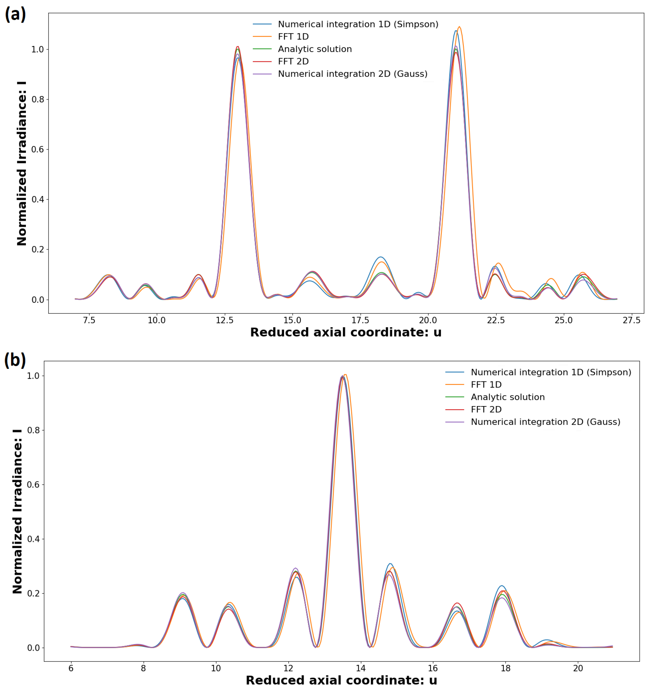
This section shows the numerical results obtained through the methods described above. The calculations were performed on a computer with 16.0 GB RAM memory and an 11th Gen Intel(R) Core(TM) i7-1165G7 @ 2.80 GHz processor. Figure 3 shows a comparison between the irradiance distributions along the optical axis as obtained for the Fibonacci and Triadic Cantor zone plates. Figure 3a shows the normalized axial irradiance for the Fibonacci zone plate of order $S=8$. As can be seen, the irradiance provided by all methods shows a bifocal behavior, as expected according to the design characteristics of the lens reported in previous works. Similarly, the irrandiance for the case of the Triadic Cantor zone place of order S = 3 is shown in Figure 3b. For both lenses, the solutions obtained from the one-dimensional methods are contrasted to a greater extent from the analytical solution, than the solutions obtained using the two-dimensional methods.

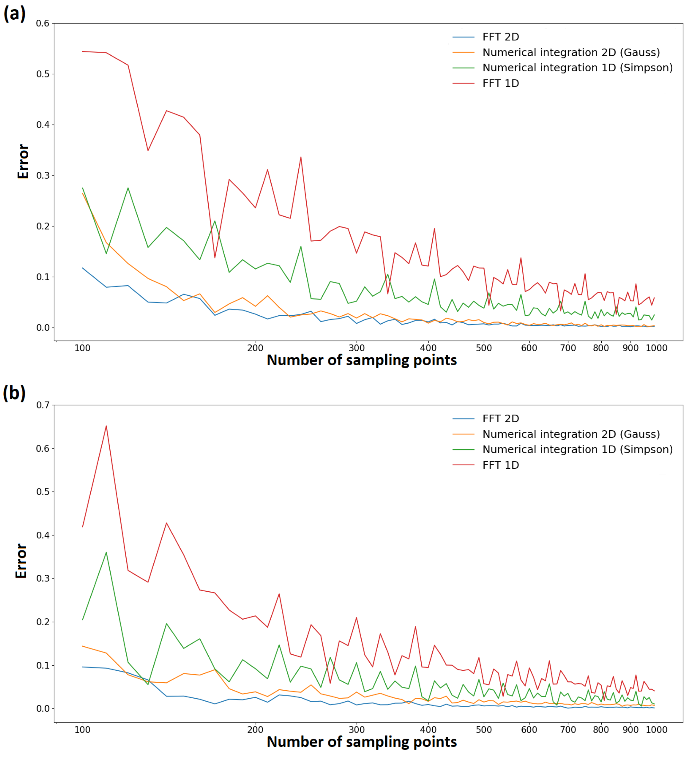
The calculations were performed for different numbers of sampling points (N) from $N=100$ to $N=1000$ in steps of $\Delta N=10$, used in the resolution of the Fresnel integral. In the case of two-dimensional methods, this quantity corresponds to the number of points for each integration variable, resulting in a sampling array of N × N. For each of these values, the relative error shown by each calculation method was determined. This relative error is defined as,

$$error=\frac{{\sum }_{i=1}^M|I_{analitycs}\left(u_i\right)-I_{numerical}\left(u_i\right)|}{{\sum }_{i=1}^M{I}_{analitycs}\left(u_i\right)}$$

(9)

where $I_{analitycs}$ is the irradiance calculated analytically, $I_{numeric}$ is the irradiance obtained by each numerical method, and M is the number of points on the optical axis where the irradiance I was calculated.

As can be seen in Figure 4, the error rate for the four methods decreases as the number of sampling points increases. The two-dimensional methods, 2D FFT and Numerical Integration by Gauss, present a fairly similar error rate for most values of N used. However, the one-dimensional methods (1D FFT and Simpson’s numerical integration) show a higher error rate than the 2D methods. This trend is the same for the Fibonacci lens of order $S=8$ (see Figure 4a), as for the triadic Cantor lens of order $S=3$ (see Figure 4b). This is due to the two-dimensional discretization of the integration domain. In cartesian coordinates this discretization provides a greater number of sampling points for the radial coordinate than the number of test points used in the one-dimensional methods, increasing the accuracy of the calculation.

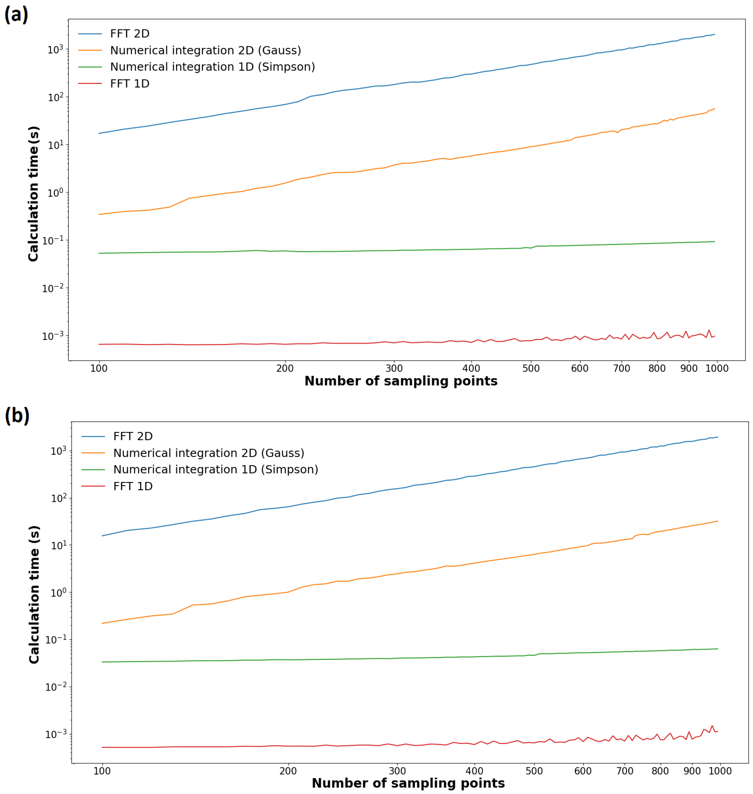
The comparative analysis of the computation time used by the one dimension and two dimensions methods was carried out, for the Fibonacci lens $S=8$ and Triadic Cantor lens $S=3$. As shown in Figure 5, the computation times were less than 1 s for the one-dimensional methods, while for 2D methods the time required is higher. The calculation time needed by the Gauss numerical integration method went from 0.1 to 60 s, and for the 2D FFT case, went from 21 s to 23.3 min. The increase in the computation time is justified by the increase in the number of evaluations of the function that contrasts with the 1D methods. Gauss’ numerical method only performs the numerical calculation of an integral for each u. At the same time, 2D FFT calculates the irradiance in the plane perpendicular to the optic axis for each value of u, which results in the processing of larger dimensional arrays. This behavior in computation time is similar for both lenses. This shows the consistency of the methods used.

4. Conclusions

Numerical integration methods play an important role in the study of the focusing properties of diffractive lenses. From the comparative analysis carried out in this work, it can be concluded that the Gauss method presents the best balance between accuracy and calculation time among the studied methods if our main interest is to know the distribution of the axial irradiance. In applications where transversal irradiance is required, for example vortex lenses used for optical trapping, it would be more convenient to use the 2D FFT because for each value of the reduced axial coordinate where the axial irradiance is calculated the 2D FFT also gives us the transversal irradiance distribution. One-dimensional methods present an acceptable error in many applications, and their computation time is the shortest. The Simpson’s method has a lower error than 1D FFT, but also a higher computation time. However, both of these methods are limited to diffractive elements with radial symmetry.

This analysis could be useful to decide which numerical method would be more convenient to solve the Fresnel diffraction integral, depending on the structure being studied. It could help us to predict the error when calculating the irradiance distribution of more complex diffractive lenses, where the Fresnel integral would be difficult to solve analytically.