An Inverse Optimal Value Approach for Synchronously Optimizing Activity Durations and Worker Assignments with a Project Ideal Cost

Abstract

Most companies survive the pain of cost and schedule overruns because of inaccurate project activity time settings. In order to deliver a project with a target cost and on schedule, this research proposes an inverse optimal value approach to optimize activity durations and the corresponding worker assignments synchronously to make the optimal project cost infinitely close to an ideal cost. The leader model reflects cost orientation and adjustability of activity durations, the follower model reflects the complexity of activity sequence, critical path completion time, cost pressure, skill matching, energy consumption, and other costs. Through upper-level and lower-level feedback and interaction of activity durations and worker assignments it is possible to deliver a project with an ideal cost. With considerations of the mathematical model characteristics of bi-level programming, nonlinearity, NP hard, and MAX functions, an improved genetic algorithm combining adaptive artificial fish swarms is designed. From the comparison results of random examples and an actual example, the error rate of the optimal value of the improved algorithm is acceptable. Numerical experiments show that the inverse optimal approach can deliver a project without delay and with an ideal cost. The inverse optimization method is more in line with the idea of target management, and can help managers achieve the purpose of cost control.

1. Introduction

Projects are responsible for almost 30% of the world’s economic activity; lots of companies are project-based companies. Nowadays, inadequate management of project overruns is growing. Most companies survive the pain of cost and schedule overruns [1]. According to a survey by the Master of Project Academy, project schedule delays and project cost overruns account for more than 50% of the issues that organizations face. Because of bad activity duration estimations and activity–worker assignments, cost overruns and delivery delays get out of control [2]; they are the biggest obstacles to the survival and development of a project-based company. The good news is that a project-cost-management problem with adjustable activity durations has attracted the attention of researchers [3].

A project duration is the total length of time a specific project takes to complete based on the activity of logical sequences and durations. Activity durations are key factors affecting total cost and project delivering time [4]. For duration estimations, both industries and academia pay great attention to the problem of how much time to spend on activities. Generally, a duration of an activity is calculated with statistical methods based on the historical data of completed activities [5]. There are different tools for estimating durations such as three-point estimation, parametric estimation, analogous estimation, and bottom-up estimation methods. Scholars consider uncertainty, risk, labor productivity, and disruptive factors when estimating durations [6]. Activity durations calculated using the above methods, which are mainly forward methods, that are only based on activity time information, they cannot guarantee to deliver a project with an ideal cost and within the duration requirement.

Furthermore, the following human factors, such as “student syndrome”, “Murphy’s law” and “Parkinson’s law”, make a project delay happen frequently [7]. People always procrastinate and postpone the task activities, and will not work hard to complete the task until the last moment. When they have enough time to finish one task, they will involuntarily reduce their work efficiency or spend time doing other things, resulting in the waste of project time. Parkinson’s Law incorporates laziness, procrastination, and self-protection against reduced deadlines in the future. Precise and strictly enforced activity-completion-time standards based on preset project goals are an important way to overcome the above human factor deficiencies [8].

Project worker assignment decisions involve the determination of optimal allocations of workers to activities [9]. A systems view of worker-assignment problems has been researched [10] with models such as the multi-task assignment model [11], task matching model [12], multi-criteria decision-making model of employee assignment [13], multi-objective optimization model for task assignment [14], assignment problem with historical data [15], maintenance workforce assignment [16], and multi-skilled personnel assignment problem [17]. All of them are forward optimization models, these methods are often used to solve assignment plans with the maximum benefit or the minimum cost under the condition that the parameters of the model are known and unchanged. They follow forward optimization methodology, and seek to compute optimal assignment decisions given fixed time parameters matrix. However, in practice, delivery date and total cost are preset and unchangeable. It is not a problem of original optimization, which is given an objective, a set of constraints, and fixed model parameters to pursue an optimal decision with minimum costs, whether the minimum costs are affordable or not. It is an inverse optimal value problem, through reverse thinking, based on reverse optimization of the time parameters of the model, so as to make the optimal solution of the original model as close as possible to the given target value.

An inverse optimization method provides an effective mechanism for transforming system parameters to obtain goals. It can be classified as an inverse optimization problem or an inverse optimal value problem. In an inverse optimization framework, the solution to the problem is known. The unknown are the model parameters. Inverse optimization takes decisions or an ideal objective function value as input and determines an objective, or constraints that render these decisions or an ideal objective function value either approximately or exactly optimal. There are two typical surveys of inverse optimization [18,19], which can give us a theory and application framework of inverse optimization methodologies. An inverse optimal value problem is a kind of inverse optimization problem, it determines the reverse-inferred parameters to make the objective function value of the corresponding forward model closest to a desired objective function value [20]. Li presents an evolutionary algorithm based on dynamic weighted aggregation methods for the multi-criterion inverse optimal-value problem [20], in order to solve the inverse optimal-value model, complementarity and relaxation conditions of the low-level problems are applied to the high-level problem through a penalty function [21]. Zhang et al. proposed an inverse optimization method for human error downtime inferring and designed a hybrid single-parent genetic particle algorithm to solve it [22]. Inverse optimization algorithms can be divided into exact algorithms and intelligent algorithms [23,24]. In terms of accurate algorithms, there are mainly bi-level programming methods and penalty function methods. Although the exact solution method can theoretically get optimal solutions, it is only applicable to small-scale problems. Researchers made progress on a single-objective linear programming inverse optimization [24], nonlinear inverse optimization [25], partial inverse assignment problem [26], multi-objective inverse optimization model [27], data-driven inverse optimization [28], robust inverse optimization [29], inverse optimization with noisy data [30], inverse mixed-integer optimization [31], and so on. Inverse optimizations related to our research are: inverse optimization for objective selection [32], inverse optimization for cost functions [33], inverse optimization for key parameter identification [34], etc. Algorithms are exact algorithms and intelligent algorithms; exact algorithms are a penalty function method based on a bi-level optimization model [35] and an evolutionary algorithm [36]. It needs to be emphasized, that inverse optimization methods have been applied to target management problems [36]. It also needs to be emphasized, that the tractability of an inverse optimization problem depends on the complexity of the forward model and the desired properties sought in the inverse model. Different problems require different problem characteristics, leading to many different inverse models and corresponding solutions. Different transformation mathematical formulas and algorithms are needed according to mathematical characteristics of forward models.

Existing research on inverse optimization theories and methodologies provides good inspiration for this research. However, the existing literature does not deal with the following requirements of project management: It is necessary to match worker skills to activity requirements; total duration is not a simply addition of all the durations, it is a MAX formula based on the critical path and each activity duration is adjustable. In order to deliver a project with an ideal cost, this research adopts the idea of the inverse optimal value method, driven by an ideal cost for delivering a project, to deduce decisions of worker–activity-duration. Based on a 0–1 mixed-integer nonlinear bi-level programming model with MAX formulas, the leader model pursues delivering a project with a desired cost by the minimum distance between the project cost of a forward problem based on adjusted preferred duration and a desired cost. The follower model minimizes the project cost based on initial durations. A hybrid artificial fish swarm genetic algorithm is used to solve the model.

This research uses an inverse optimal value method, to synchronize and optimize durations and worker assignments to deliver a project with an ideal cost. It provides a new idea and a new method for the worker assignment research It has the following innovation points: (1) This research combines push and pull strategies to make them complement each other to deliver a project within an ideal cost. The push strategy is used to determine original durations, and the pull strategy to give adjusted preferred durations based on an ideal cost. It provides a novel way to solve duration optimization problems driven by a preset value. (2) This research combines a genetic algorithm and an artificial fish algorithm to foster strengths and circumvent weaknesses with considerations of nonlinearity, NP difficulty, and MAX functions. Based on our comparisons, the error rate of the optimal value of the improved algorithm is acceptable.

The structure of this research is as follows. In Section 1, we give an introduction and review the literature on project worker assignments and inverse optimization problems. In Section 2, we construct a mathematical model of the inverse optimal value method. In Section 3, a self-adaptation hybrid artificial fish-swarm genetic algorithm is designed. Section 4 provides an application example of numerical analysis. Section 5 concludes the study.

2. Mathematical Formulations

2.1. Analysis of an Inverse Optimal Value Model of Project Activity–Worker Assignment

An inverse optimization method is essentially different from a forward optimization method. A forward optimization method is to find a point in the feasible region of the model under the condition that all resource parameters are fixed, so that the objective function value corresponding to the point is optimal. An inverse optimization method is a logically opposite problem to the forward optimization method. Its main idea is an “inverse” activity, that is, under the condition of knowing a certain criterion (desired solution or objective function value), the activity of making the predetermined criterion becomes the optimal result (optimal solution or optimal objective value) by adjusting the resource parameters within the feasible range. An inverse optimal value method of project activity–worker assignment is an optimization method in which the desired objective function value is known, and the aim is to find new activity durations which can make the desired value the optimal value of the forward model under the new activity durations and new activity–worker assignment themes.

An inverse optimal value method corresponds to a forward optimization model. In a forward model, the parameters in the model remain unchanged, and it is an activity of finding a solution that makes the objective function value optimal in the feasible region. In an inverse optimal value method on the contrary, the desired objective function value is often considered to be the optimal value of the model, by adjusting the parameter to make the desired objective function value optimal. It is an activity of finding the best solution to a problem by working backwards from the desired outcome. It involves starting with the desired result and then working backwards to determine the best way to achieve the desired result.

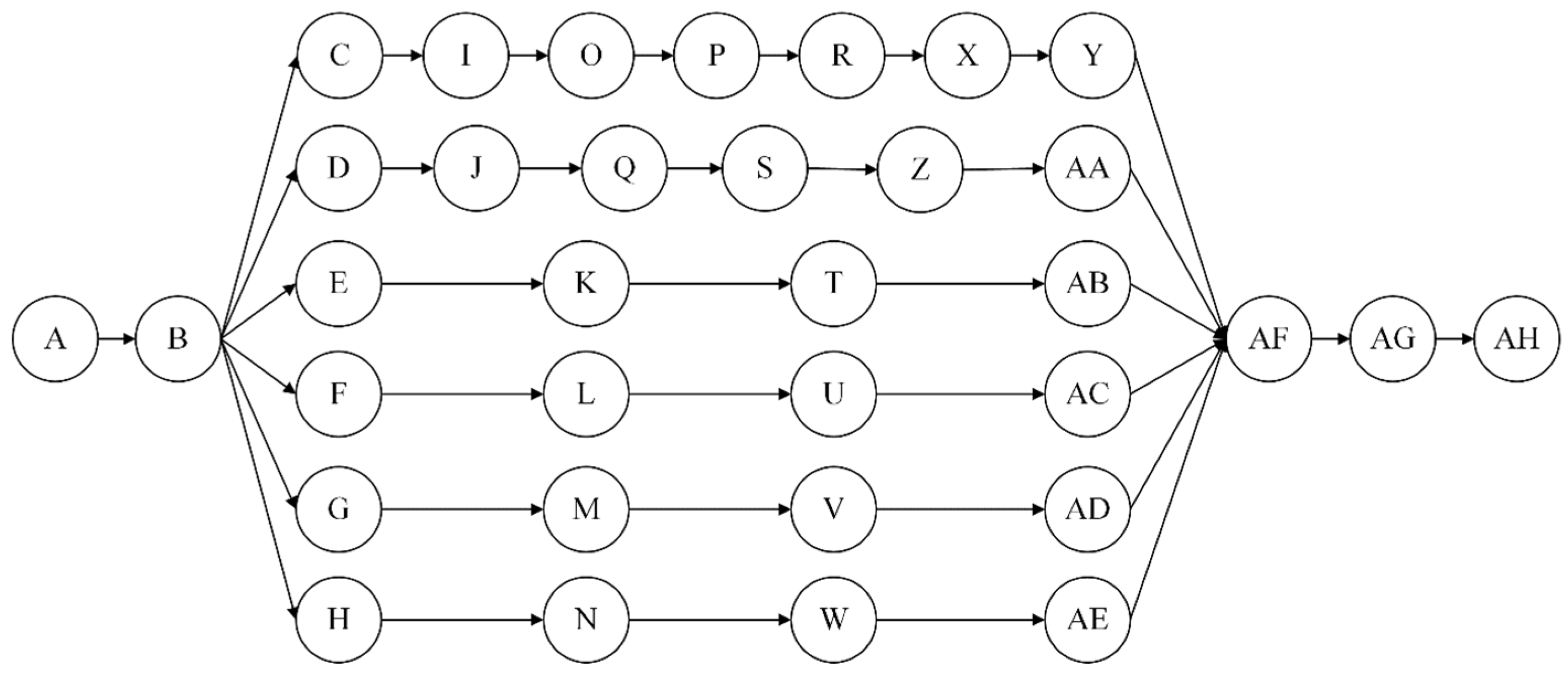
This research defines the “activity–worker” inverse assignment problem as follows: Based on the forward optimization model of “activity–worker” assignment, through reverse thinking, starting from the given target cost, through adjusting activity durations, the aim is to make the optimal objective value of the model the desired value. The “activity–worker” reverse assignment method of a project combines the idea of objective management, a 0–1 integer programming method, and a reverse optimal value method, through the cost objective management of the project, to achieve the goal of controlling the cost, and to obtain the corresponding “activity–worker” assignment scheme. The methodology framework is shown in Figure 1.

2.2. Problem Description

A project task assignment is the activity of assigning tasks to individuals in order to deliver a project. This type of assignment typically involves assigning specific tasks to individuals, as well as assigning deadlines. It also involves setting expectations for the completion time of each activity, such as the timeline for completion. A forward model is to find worker assignments of a project with constrains of skill matching, labor cost budgets, delivering time requirements, and multi-tasks; the minimum total cost of performing all activities is based on initial durations. However, the optimal objective value is not satisfying, as the duration is adjustable. Then, the goal of an inverse optimal value model is to determine parameters of a forward model that render an ideal cost exactly to be the optimal objective function value with respect to the forward model structure. A desired total cost is treated as an input variable in the inverse optimal value model, and the activity durations and worker assignments are treated as output variables. Decision makers want to deliver a project with a desired cost with some constrains. “Duration–worker–activity” assignment decisions need to be made. Activities of a project have the characteristics of order (order of precedence, parallel), heterogeneity, different durations with different workers, and materials needed are not changeable, whereas duration is changeable. Workers of a project have the characteristics of heterogeneity of skills. Time can be self-controlled within a certain range. A worker with multiple tasks not performed at the same time is determined to show delay tendencies, “student syndrome” et al., which are benchmarking criteria.

2.3. Model Assumptions

By optimizing and adjusting the operation time parameters, the actual total cost of the project is as close as possible to the expected cost target of the enterprise, and the corresponding assignment scheme and operation time parameters are obtained. The model assumptions are as follows: (1) The primary concern of a project-based company is cost; a project must be delivered strictly with a desired cost, the cost must be strictly enforced, and no overspending is allowed. (2) In order to show respect for the workers, each worker reported the estimated working time on each activity prior to the personnel assignment decision. Due to different efficiencies of workers, activity durations of different workers with different activities are different. The above estimated working time on each activity is called initial activity duration. (3) Decision makers give a primary activity–worker assignment theme based on the initial durations with the purpose of minimizing the total cost. (4) For quality control reasons, the materials for a project are beyond the decision scope; decision makers cannot reduce cost from the perspective of materials. (5) Activity durations not only affect total duration of the whole project, but also affect total cost of a project. When the minimum total cost based on the initial durations is higher than the desired cost, it is necessary to readjust activity durations to reduce total cost. (6) For the human-factor reasons mentioned before, activity durations are adjustable [34]. (7) Due to skill constraints, workers may only be able to complete one or several tasks, or maybe unable to perform tasks because they do not meet the skill requirements.

2.4. Mathematical Symbols

The mathematical symbols and meanings are shown in

Table 1. Mathematical symbol and their meanings.

Variable	Variable Meaning
$x_{ik}$	A binary variable equal to 1 if, and only if, worker $k$ is assigned to activity $i$
$t_{ik}$	Activity duration if, and only if, worker $k$ is assigned to activity $i$
$c^u$	Upper control limit of worker cost
$t^u$	Upper control limit of project duration
$c_{ik}$	Cost per unit if worker $k$ is assigned to activity $i$
${\theta }_j$	$j_{th}$ energy cost coefficient
s	The s-th skill
$\underset{n_{is}}{\to }$	Indicates the skill demand vector of the i-th activity. When $n_{is}$= 1, it means that the worker must have the s-th skill to work at the i-th activity; when $n_{is}$= 0, it means the worker is not required to have the s-th skill for the activity
$\underset{h_{ks}}{\to }$	Represents the skill vector of the k-th worker. When $h_{ks}$= 1, it means the worker has the s-th skill; when $h_{ks}$= 0, it means the operator does not have the s-th skill
$I_{\tau }$	Collection of activities in the $\tau$th tandem path from start to end $\tau =1,2,\dots ,e$
${\mathsf{\Omega }}_{\tau }^i$	Collection of all activities in tandem path $\tau$th
${\varphi }_i$	Collection of all activities prior to activity $i$, on the same tandem path $\tau$th
$f^{*}$	Ideal target cost
$\beta$	Other cost coefficient

.

2.5. Forward Activity–Duration Assignment Model

In the forward worker-activity assignment model (1), the decisions are activity–worker assignment themes based on the initial activity duration matrixes to pursue the minimum cost of the project.

$$\underset{ }{\min }{\displaystyle \sum }_{i=1}^m{\displaystyle \sum }_{k=1}^n{c}_{ik}{x}_{i,k}{t}_{i,k}+\left({\displaystyle \sum }_{j=1}^u{\theta }_j+\beta \right)\times \underset{\tau =1,2,\dots ,e}{\max }\left\{{\displaystyle \sum }_{i\in I_{\tau }}{\displaystyle \sum }_{k=1}^n{x}_{i,k}{t}_{i,k}\right\}$$

$$s.t. \underset{\tau =1,2,\dots ,e}{\max }\left\{{\displaystyle \sum }_{i\in I_{\tau }}{\displaystyle \sum }_{k=1}^n{x}_{i,k}{t}_{i,k}\right\}\le c^u$$

$${\displaystyle \sum }_{i=1}^m{\displaystyle \sum }_{k=1}^n{c}_{ik}{x}_{i,k}{t}_{i,k}\le t^u$$

$$\left({\overrightarrow{n}}_{i,s}·{\overrightarrow{h}}_{k,s}-{\displaystyle \sum }_{s=1}^S{n}_{i,s}\right)·x_{i,k}\ge 0$$

(1)

$${\displaystyle \sum }_{k=1}^n{x}_{i,k}=1,i=1,2,\dots ,m$$

$$\begin{array}{c}\left[\underset{\tau \in {\varphi }_{i_1}}{\max }\left\{{\displaystyle {\displaystyle \sum }_{i^1\in {\Omega }_{\tau }^{i_1}}}{\displaystyle {\displaystyle \sum }_{k=1}^n}{x}_{i^1,k}{t}_{i^1,k}\right\}-\left(\underset{\tau \in {\varphi }_{i_2}}{\max }\left\{{\displaystyle {\displaystyle \sum }_{i^2\in {\Omega }_{\tau }^{i_2}}}{\displaystyle {\displaystyle \sum }_{k=1}^n}{x}_{i^2,k}{t}_{i^2,k}\right\}+{\displaystyle {\displaystyle \sum }_{k=1}^n}{x}_{i_2,k}{t}_{i^2,k}\right)\right]\hfill \\ \times \left[\underset{\tau \in {\varphi }_{i_2}}{\max }\left\{{\displaystyle {\displaystyle \sum }_{i^2\in {\Omega }_{\tau }^{i_2}}}{\displaystyle {\displaystyle \sum }_{k=1}^n}{x}_{i^2,k}{t}_{i^2,k}\right\}-\left(\underset{\tau \in {\varphi }_{i_1}}{\max }\left\{{\displaystyle {\displaystyle \sum }_{i^1\in {\Omega }_{\tau }^{i_1}}}{\displaystyle {\displaystyle \sum }_{k=1}^n}{x}_{i^1,k}{t}_{i^1,k}\right\}+{\displaystyle {\displaystyle \sum }_{k=1}^n}{x}_{i_1,k}{t}_{i_1,k}\right)\right]\le 0\hfill \end{array}$$

$$x_{i,k}\in \left\{0,1\right\}$$

In model (1): $\underset{\tau =1,2,\dots ,e}{\max }\left\{{\displaystyle \sum }_{i\in I_{\tau }}{\displaystyle \sum }_{k=1}^n{x}_{i,k}{t}_{i,k}\right\}$ is project duration based on critical path method; $\underset{}{\min }{\displaystyle \sum }_{i=1}^m{\displaystyle \sum }_{k=1}^n{c}_{ik}{x}_{i,k}{t}_{i,k}+\left({\displaystyle \sum }_{j=1}^u{\theta }_j+\beta \right)\times \underset{\tau =1,2,\dots ,e}{\max }\left\{{\displaystyle \sum }_{i\in I_{\tau }}{\displaystyle \sum }_{k=1}^n{x}_{i,k}{t}_{i,k}\right\}$ is to minimize total cost. ${\displaystyle \sum }_{i=1}^m{\displaystyle \sum }_{k=1}^n{c}_{ik}{x}_{i,k}{t}_{i,k}$ is the total labor cost. ${\displaystyle \sum }_{j=1}^u{\theta }_j\times \underset{\tau =1,2,\dots ,e}{\max }\left\{{\displaystyle \sum }_{i\in I_{\tau }}{\displaystyle \sum }_{k=1}^n{x}_{i,k}{t}_{i,k}\right\}$ is the total energy cost. $\beta \times \underset{\tau =1,2,\dots ,e}{\max }\left\{{\displaystyle \sum }_{i\in I_{\tau }}{\displaystyle \sum }_{k=1}^n{x}_{i,k}{t}_{i,k}\right\}$ are other costs based on total duration. The constraint formula $\underset{\tau =1,2,\dots ,e}{\max }\left\{{\displaystyle \sum }_{i\in I_{\tau }}{\displaystyle \sum }_{k=1}^n{x}_{i,k}{t}_{i,k}\right\}\le c^u$ means the project duration is no longer than the predefined project deliver date. Formula ${\displaystyle \sum }_{i=1}^m{\displaystyle \sum }_{k=1}^n{c}_{ik}{x}_{i,k}{t}_{i,k}\le t^u$ states the total worker cost must be less than a given labor budget. Constraint $\left({\overrightarrow{n}}_{i,s}·{\overrightarrow{h}}_{k,s}-{\displaystyle \sum }_{s=1}^S{n}_{i,s}\right)·x_{i,k}\ge 0$ states each worker satisfies activity skills requirements. Constraint formula ${\displaystyle \sum }_{k=1}^n{x}_{i,k}=1,i=1,2,\dots ,m$ means there is no activity with no workers. Constraint formula $\left[\underset{\tau \in {\varphi }_{i_1}}{\max }\left\{{\displaystyle \sum }_{i^1\in {\Omega }_{\tau }^{i_1}}{\displaystyle \sum }_{k=1}^n{x}_{i^1,k}{t}_{i^1,k}\right\}-\left(\underset{\tau \in {\varphi }_{i_2}}{\max }\left\{{\displaystyle \sum }_{i^2\in {\Omega }_{\tau }^{i_2}}{\displaystyle \sum }_{k=1}^n{x}_{i^2,k}{t}_{i^2,k}\right\}+{\displaystyle \sum }_{k=1}^n{x}_{i_2,k}{t}_{i^2,k}\right)\right]\times \left[\underset{\tau \in {\varphi }_{i_2}}{\max }\left\{{\displaystyle \sum }_{i^2\in {\Omega }_{\tau }^{i_2}}{\displaystyle \sum }_{k=1}^n{x}_{i^2,k}{t}_{i^2,k}\right\}-\left(\underset{\tau \in {\varphi }_{i_1}}{\max }\left\{{\displaystyle \sum }_{i^1\in {\Omega }_{\tau }^{i_1}}{\displaystyle \sum }_{k=1}^n{x}_{i^1,k}{t}_{i^1,k}\right\}+{\displaystyle \sum }_{k=1}^n{x}_{i_1,k}{t}_{i_1,k}\right)\right]\le 0$ means if one worker is assigned to multiple tasks, there is no time overlap among those activities.

2.6. Inverse Optimal Value Model of Activity–Worker Assignment with Duration Optimization

An inverse optimization method based on bi-level programming for worker assignment is constructed. The leader model reflects cost orientation and adjustability of activity duration; the follower model reflects the complexity of activity sequence, cost pressure, energy consumption, and environmental protection. Through upper-level and lower-level feedback and interaction of activity duration and worker assignment, the model delivers a project with an ideal cost. The inverse optimization method is more in line with the idea of target management, and can help enterprises achieve the purpose of cost control.

According to the above definition of inverse optimal value problem of project activity–worker assignment, based on a bi-level programming method, the inverse optimal model is proposed (Formula (2)). In the inverse optimal value model (2), the upper model is to pursue delivering a project with desired target cost based on optimization activity durations. The lower level is the forward optimization model of optimizing the “activity–worker” assignment scheme under the original activity duration matrix. Formula (2) is a bi-level nonlinear mixed-integer programming model. The upper-level programming problem is not only related to the upper-level decisions, but also affected by the optimal solution of the lower-level programming problem, and vice versa. Activity-duration decision variables of the upper-level optimization problem interact with the assignment scheme decision variables of the lower-level optimization problem, resulting in mutual feedback, and constant iterating, until “activity-duration-worker” triads are found to make the cost be the desired target cost. The transformation ideas of inverse optimal value method are shown in Figure 2.

Based on the literature [21], the inverse optimal value model is as follows:

$$\mathrm{leader}\mathrm{model}:\underset{t_{ik}}{\min }\left|{\displaystyle \sum }_{i=1}^m{\displaystyle \sum }_{k=1}^n{c}_{ik}{x}_{i,k}{t}_{i,k}+\left({\displaystyle \sum }_{j=1}^u{\theta }_j+\beta \right)\times \underset{\tau =1,2,\dots ,e}{\max }\left\{{\displaystyle \sum }_{i\in I_{\tau }}{\displaystyle \sum }_{k=1}^n{x}_{i,k}{t}_{i,k}\right\}-f^{*}\right|$$

$$s.t. t_0\le t_{ik}\le t_1$$

$$\mathrm{follower}\mathrm{model}:\underset{x_{ik}}{\min }{\displaystyle {{\displaystyle \sum }}_{i=1}^m}{\displaystyle {{\displaystyle \sum }}_{k=1}^n}{c}_{ik}{x}_{i,k}{t}_{i,k}+\left({\displaystyle {{\displaystyle \sum }}_{j=1}^u}{\theta }_j+\beta \right)\times \underset{\tau =1,2,\dots ,e}{\max }\left\{{\displaystyle {{\displaystyle \sum }}_{i\in I_{\tau }}}{\displaystyle {{\displaystyle \sum }}_{k=1}^n}{x}_{i,k}{t}_{i,k}\right\}$$

$$s.t. \underset{\tau =1,2,\dots ,e}{\max }\left\{{{\displaystyle \sum }}_{i\in I_{\tau }}{{\displaystyle \sum }}_{k=1}^n{x}_{i,k}{t}_{i,k}\right\}\le c^u$$

$${{\displaystyle \sum }}_{i=1}^m{{\displaystyle \sum }}_{k=1}^n{c}_{ik}{x}_{i,k}{t}_{i,k}\le t^u$$

(2)

$$\left({\overrightarrow{n}}_{i,s}·{\overrightarrow{h}}_{k,s}-{{\displaystyle \sum }}_{s=1}^S{n}_{i,s}\right)·x_{i,k}\ge 0$$

$${{\displaystyle \sum }}_{k=1}^n{x}_{i,k}=1,i=1,2,\dots ,m$$

$$\begin{array}{c}\left[\underset{\tau \in {\varphi }_{i_1}}{\max }\left\{{\displaystyle \sum }_{i^1\in {\Omega }_{\tau }^{i_1}}{\displaystyle \sum }_{k=1}^n{x}_{i^1,k}{t}_{i^1,k}\right\}-\left(\underset{\tau \in {\varphi }_{i_2}}{\max }\left\{{\displaystyle \sum }_{i^2\in {\Omega }_{\tau }^{i_2}}{\displaystyle \sum }_{k=1}^n{x}_{i^2,k}{t}_{i^2,k}\right\}+{\displaystyle \sum }_{k=1}^n{x}_{i_2,k}{t}_{i^2,k}\right)\right]\times \hfill \\ \left[\underset{\tau \in {\varphi }_{i_2}}{\max }\left\{{\displaystyle \sum }_{i^2\in {\Omega }_{\tau }^{i_2}}{\displaystyle \sum }_{k=1}^n{x}_{i^2,k}{t}_{i^2,k}\right\}-\left(\underset{\tau \in {\varphi }_{i_1}}{\max }\left\{{\displaystyle \sum }_{i^1\in {\Omega }_{\tau }^{i_1}}{\displaystyle \sum }_{k=1}^n{x}_{i^1,k}{t}_{i^1,k}\right\}+{\displaystyle \sum }_{k=1}^n{x}_{i_1,k}{t}_{i_1,k}\right)\right]\le 0\hfill \end{array}$$

$$x_{i,k}\in \left\{0,1\right\}$$

In model (2) the objective function formula $\underset{t_{ik}}{\min }\left|{\displaystyle \sum }_{i=1}^m{\displaystyle \sum }_{k=1}^n{c}_{ik}{x}_{i,k}{t}_{i,k}+\left({\displaystyle \sum }_{j=1}^u{\theta }_j+\beta \right)\times \underset{\tau =1,2,\dots ,e}{\max }\left\{{\displaystyle \sum }_{i\in I_{\tau }}{\displaystyle \sum }_{k=1}^n{x}_{i,k}{t}_{i,k}\right\}-f^{*}\right|$ is to minimize the distance between the optimized cost and the desired target cost. The constraint formula $t_0\le t_{ik}\le t_1$ means a feasible adjustable region of activity durations. The other formula, that is the follower level model, is exactly the same as the forward model (1).

3. Self-Adaptation Hybrid Artificial Fish Swarm Genetic Algorithm for an Inverse Optimization Model

Formula (2) is a bi-level nonlinear mixed-integer programming model. The upper-level programming problem is not only related to the upper-level decisions, but also affected by the optimal solution of the lower-level programming problem, which is affected by the lower-level decision variables. Additionally, the two-level decision variables interact with each other, leading to a rapid expansion of the solution space, and the computational efficiency is obviously very low when using an exact algorithm to solve the model.

The inverse optimal value model contains two kinds of decision variables, task–worker assignments and activity durations; they affect each other, leading to a sharp expansion of the solution space. A genetic algorithm with high optimization efficiency, simple operation, and robust performance is applied on activity–worker assignments and increases learning operation to accelerate the convergence of the algorithm. An artificial fish algorithm with a strong ability to overcome local extreme acts on operation-time-parameter variables to improve the accuracy of the algorithm solution. In order to deal with different requirements on algorithm parameters during different periods, we propose a parametric adaptive hybrid artificial fish population genetic algorithm based on linear functions. A genetic algorithm that introduces the learning mechanism between individuals in the population is used to solve the 0–1 integer programming in the lower level. Combined with the advantages of artificial fish swarm algorithm, such as parallel calculating, global optimization, and the ability to quickly jump out of the local extreme point, the artificial fish swarm algorithm is used to solve the continuous variable operation time optimization problem of upper-level planning. The algorithm flow is shown in Figure 3.

4. Numerical Examples

4.1. Project Background and Parameters

Company H is a project-based company; it undertakes an equipment overhaul project. According to the project contract, the material resources such as equipment spare parts involved in the project are provided by company A. Company A is the first party according to the project contract. As the second party, company H is mainly responsible for the human resource assignment, performance management, and other work related to the project. For example, company H needs to bear the energy and other costs related to the project duration during the overhaul. The contract stipulates that the project delivery time must be strictly followed, otherwise the liquidated damages under the contract are huge. From company H’s point of view, in order to maintain the survival and development of the enterprise, after lots of investigations, this project should be delivered with the desired target cost, otherwise it is difficult to maintain the normal operation and sustainable development of the company. Through the definition of the overall project scope of the project and the analysis of activities, the network planning diagram of activities of the project is given, as shown in Figure 4. There are 38 activities in a project and there are 30 workers available to be assigned in the project. Company H obtains the original activity-duration matrix through investigation of all the workers who are intended to participate in the project. In addition, based on lots of research, company H gives the labor wage coefficient according to the labor market, the company’s development status, and the complexity of activities. Based on the analysis of the task difficulty of the project activities and the opinions of many experts, the labor cost coefficient of each activity in the project is given. According to the value of related energy, the cost coefficients of different energies are given. Considering other costs of the project, the cost coefficient of other costs per unit time is given through the investigation of local experts. The ideal cost of CNY 360,000 is given by the top manager of the company, company H needs to deliver the project with the target cost by optimizing worker assignments and durations together. Project parameters are shown in Table 2, Table 3, Table 4, Table 5 and Table 6.

4.2. Calculation Based on an Adaptive Hybrid Artificial Fish Swarm Genetic Algorithm

According to the proposed “activity–worker” inverse assignment model (2), the feasible range of the activity durations of each worker on each activity is given. The parameter adaptive hybrid artificial fish swarm genetic algorithm based on a linear function is used to solve the inverse optimal value model; the algorithm parameter settings are shown in Table 7, and the algorithm program is written in MATLAB version R2018b Since the MATLAB solver implements and tests algorithms easily, they debug easily. Most of the calculations are based on MATLAB, without loss of generality, this research uses the MATLAB solver to do the calculations using an Intel (R) Core (TM) i5-10210U CPU @ 1.60 GHz 2 computer with a 10 GHz processor, 8 GB of RAM, and Windows 10 64-bit operating system to run the programs.

Based on MATLAB R 2018b, after 10 iterations the results meet the termination condition, the running time is 109.458 s. The total cost of 1.0083 × 10⁻⁴ is less than the ideal cost, which means that the project is delivered with an ideal cost. The iteration diagram for solving the inverse optimal value model is shown in Figure 5.

Table 2. Labor-cost coefficient.

	Activity	1	2	3	4	5	6	7	8	9	10	11	12	13	14	15	16	17	18	19	20	21	22	23	24	25	26	27	28	29	30
Worker
1		150	136	191	142	125	221	206	155	143	131	234	250	140	190	99	240	221	194	241	251	260	261	249	151	248	201	252	218	163	257
2		117	107	150	112	100	173	163	120	112	102	184	196	110	149	77	189	173	153	189	197	205	204	195	119	194	157	199	172	127	202
3		150	136	191	142	125	221	206	155	143	131	234	250	140	190	98	241	220	193	242	251	261	261	248	150	247	201	250	218	164	256
4		151	138	194	144	127	225	210	156	144	131	238	253	143	193	100	245	223	197	244	255	265	263	252	154	250	202	257	222	164	261
5		81	74	104	77	68	121	113	84	77	70	127	135	76	103	103	131	120	106	130	136	142	141	135	82	134	108	137	119	88	140
6		125	115	162	120	106	187	175	130	120	109	198	210	119	160	83	203	186	164	203	212	220	219	209	128	208	168	213	185	137	218
7		119	109	153	114	100	177	166	123	114	103	188	199	112	152	79	193	176	156	192	201	208	207	198	121	197	159	202	175	129	205
8		140	128	180	134	118	209	196	145	134	122	221	235	133	179	93	227	208	183	226	237	246	244	234	143	232	188	238	206	153	242
9		150	136	191	142	125	221	206	155	143	131	234	250	140	190	99	241	220	193	242	251	261	261	248	150	247	201	250	218	164	256
10		131	120	136	126	111	196	183	136	126	114	208	220	124	114	87	213	195	172	212	222	231	229	219	134	218	176	224	193	142	227
11		125	115	162	120	106	187	175	130	120	109	198	210	119	160	83	203	186	164	203	212	220	219	209	128	208	168	213	185	137	217
12		99	91	128	95	84	148	139	103	95	87	157	167	94	127	66	161	147	181	190	197	196	187	115	186	150	191	165	122	194	220
13		139	127	179	133	117	207	194	144	133	121	219	233	131	177	92	225	206	182	224	235	244	242	232	142	230	196	236	204	151	240
14		112	102	144	107	95	167	156	116	107	98	177	188	106	143	74	182	166	147	181	190	197	196	187	115	186	150	191	165	122	194
15		99	91	128	95	84	148	139	103	95	87	157	167	94	127	66	161	147	130	161	168	175	173	166	102	165	133	169	145	103	172
16		134	123	173	128	113	200	187	139	128	117	212	225	127	171	89	218	199	176	217	227	235	234	224	137	222	180	228	197	146	232
17		125	114	161	119	105	186	174	129	119	109	197	209	118	159	83	202	185	163	202	211	219	218	208	127	207	167	212	184	136	215
18		107	98	137	102	90	159	149	111	102	93	169	179	101	136	71	173	158	140	172	180	187	186	178	109	177	143	182	157	116	185
19		127	116	163	121	107	189	177	131	121	110	200	212	120	162	84	206	131	166	205	214	223	221	212	130	210	170	216	187	138	219
20		131	119	168	125	111	195	183	135	125	114	207	219	124	167	87	212	194	171	211	221	230	228	218	134	217	175	222	192	143	226
21		132	121	170	126	112	197	184	137	126	115	209	221	125	169	87	214	196	173	213	223	232	230	220	135	219	177	225	194	144	229
22		119	109	153	114	102	176	168	123	115	104	188	201	113	152	80	193	176	156	193	201	210	209	200	123	198	161	203	175	130	207
23		119	108	151	114	100	178	165	122	114	104	187	199	111	153	79	194	174	157	192	202	208	203	197	121	198	159	202	174	129	207
24		88	79	113	83	74	128	120	91	83	76	136	145	81	112	107	141	129	115	140	146	152	152	145	89	143	116	147	128	95	149
25		128	117	165	124	108	124	182	134	124	113	203	217	121	165	87	210	193	169	209	219	227	226	216	132	215	174	220	190	141	224
26		133	122	172	127	112	199	186	138	127	116	211	224	126	170	88	217	188	166	216	226	234	233	223	136	221	189	227	196	145	222
27		106	97	138	103	91	160	150	112	103	94	170	187	100	135	72	170	160	148	170	190	176	185	179	109	177	142	182	157	116	185
28		100	92	129	96	85	149	140	104	96	88	158	168	95	128	67	162	148	161	162	169	176	174	168	100	162	135	168	146	103	165
29		150	137	193	143	127	223	209	155	143	131	236	250	142	191	100	240	220	195	240	250	260	261	245	156	249	200	253	218	160	262
30		130	117	168	125	110	193	181	134	126	113	208	219	135	161	90	200	190	168	209	219	227	226	215	134	214	170	225	195	140	222
31		90	83	115	86	76	125	126	90	85	90	140	140	88	111	107	141	168	130	116	150	150	150	150	145	90	160	130	120	180	156
32		92	84	117	88	78	134	126	95	88	81	142	150	87	116	62	146	134	119	145	152	157	156	150	94	149	121	153	133	100	155
33		104	95	134	99	87	156	146	108	99	90	166	176	98	133	68	170	155	137	169	177	184	183	175	106	174	140	179	154	113	182
34		114	104	146	109	97	169	158	118	109	100	179	190	108	145	76	184	168	149	183	192	199	198	189	117	188	152	193	167	124	196
35		119	109	152	114	101	176	165	123	114	104	186	198	112	151	79	191	175	155	191	199	207	206	197	121	196	159	201	174	129	204
36		127	116	166	121	106	193	180	132	121	110	205	218	120	164	82	211	182	160	210	220	228	227	217	130	215	183	221	190	139	216
37		130	117	173	123	107	203	189	135	123	111	216	230	122	171	80	220	200	175	220	230	240	241	225	136	229	180	233	198	140	240
38		102	94	131	98	87	151	142	106	98	90	160	170	97	130	69	164	150	133	164	171	178	176	169	105	168	136	172	148	111	175

Table 2. Labor-cost coefficient.

	Activity	1	2	3	4	5	6	7	8	9	10	11	12	13	14	15	16	17	18	19	20	21	22	23	24	25	26	27	28	29	30
Worker
1		150	136	191	142	125	221	206	155	143	131	234	250	140	190	99	240	221	194	241	251	260	261	249	151	248	201	252	218	163	257
2		117	107	150	112	100	173	163	120	112	102	184	196	110	149	77	189	173	153	189	197	205	204	195	119	194	157	199	172	127	202
3		150	136	191	142	125	221	206	155	143	131	234	250	140	190	98	241	220	193	242	251	261	261	248	150	247	201	250	218	164	256
4		151	138	194	144	127	225	210	156	144	131	238	253	143	193	100	245	223	197	244	255	265	263	252	154	250	202	257	222	164	261
5		81	74	104	77	68	121	113	84	77	70	127	135	76	103	103	131	120	106	130	136	142	141	135	82	134	108	137	119	88	140
6		125	115	162	120	106	187	175	130	120	109	198	210	119	160	83	203	186	164	203	212	220	219	209	128	208	168	213	185	137	218
7		119	109	153	114	100	177	166	123	114	103	188	199	112	152	79	193	176	156	192	201	208	207	198	121	197	159	202	175	129	205
8		140	128	180	134	118	209	196	145	134	122	221	235	133	179	93	227	208	183	226	237	246	244	234	143	232	188	238	206	153	242
9		150	136	191	142	125	221	206	155	143	131	234	250	140	190	99	241	220	193	242	251	261	261	248	150	247	201	250	218	164	256
10		131	120	136	126	111	196	183	136	126	114	208	220	124	114	87	213	195	172	212	222	231	229	219	134	218	176	224	193	142	227
11		125	115	162	120	106	187	175	130	120	109	198	210	119	160	83	203	186	164	203	212	220	219	209	128	208	168	213	185	137	217
12		99	91	128	95	84	148	139	103	95	87	157	167	94	127	66	161	147	181	190	197	196	187	115	186	150	191	165	122	194	220
13		139	127	179	133	117	207	194	144	133	121	219	233	131	177	92	225	206	182	224	235	244	242	232	142	230	196	236	204	151	240
14		112	102	144	107	95	167	156	116	107	98	177	188	106	143	74	182	166	147	181	190	197	196	187	115	186	150	191	165	122	194
15		99	91	128	95	84	148	139	103	95	87	157	167	94	127	66	161	147	130	161	168	175	173	166	102	165	133	169	145	103	172
16		134	123	173	128	113	200	187	139	128	117	212	225	127	171	89	218	199	176	217	227	235	234	224	137	222	180	228	197	146	232
17		125	114	161	119	105	186	174	129	119	109	197	209	118	159	83	202	185	163	202	211	219	218	208	127	207	167	212	184	136	215
18		107	98	137	102	90	159	149	111	102	93	169	179	101	136	71	173	158	140	172	180	187	186	178	109	177	143	182	157	116	185
19		127	116	163	121	107	189	177	131	121	110	200	212	120	162	84	206	131	166	205	214	223	221	212	130	210	170	216	187	138	219
20		131	119	168	125	111	195	183	135	125	114	207	219	124	167	87	212	194	171	211	221	230	228	218	134	217	175	222	192	143	226
21		132	121	170	126	112	197	184	137	126	115	209	221	125	169	87	214	196	173	213	223	232	230	220	135	219	177	225	194	144	229
22		119	109	153	114	102	176	168	123	115	104	188	201	113	152	80	193	176	156	193	201	210	209	200	123	198	161	203	175	130	207
23		119	108	151	114	100	178	165	122	114	104	187	199	111	153	79	194	174	157	192	202	208	203	197	121	198	159	202	174	129	207
24		88	79	113	83	74	128	120	91	83	76	136	145	81	112	107	141	129	115	140	146	152	152	145	89	143	116	147	128	95	149
25		128	117	165	124	108	124	182	134	124	113	203	217	121	165	87	210	193	169	209	219	227	226	216	132	215	174	220	190	141	224
26		133	122	172	127	112	199	186	138	127	116	211	224	126	170	88	217	188	166	216	226	234	233	223	136	221	189	227	196	145	222
27		106	97	138	103	91	160	150	112	103	94	170	187	100	135	72	170	160	148	170	190	176	185	179	109	177	142	182	157	116	185
28		100	92	129	96	85	149	140	104	96	88	158	168	95	128	67	162	148	161	162	169	176	174	168	100	162	135	168	146	103	165
29		150	137	193	143	127	223	209	155	143	131	236	250	142	191	100	240	220	195	240	250	260	261	245	156	249	200	253	218	160	262
30		130	117	168	125	110	193	181	134	126	113	208	219	135	161	90	200	190	168	209	219	227	226	215	134	214	170	225	195	140	222
31		90	83	115	86	76	125	126	90	85	90	140	140	88	111	107	141	168	130	116	150	150	150	150	145	90	160	130	120	180	156
32		92	84	117	88	78	134	126	95	88	81	142	150	87	116	62	146	134	119	145	152	157	156	150	94	149	121	153	133	100	155
33		104	95	134	99	87	156	146	108	99	90	166	176	98	133	68	170	155	137	169	177	184	183	175	106	174	140	179	154	113	182
34		114	104	146	109	97	169	158	118	109	100	179	190	108	145	76	184	168	149	183	192	199	198	189	117	188	152	193	167	124	196
35		119	109	152	114	101	176	165	123	114	104	186	198	112	151	79	191	175	155	191	199	207	206	197	121	196	159	201	174	129	204
36		127	116	166	121	106	193	180	132	121	110	205	218	120	164	82	211	182	160	210	220	228	227	217	130	215	183	221	190	139	216
37		130	117	173	123	107	203	189	135	123	111	216	230	122	171	80	220	200	175	220	230	240	241	225	136	229	180	233	198	140	240
38		102	94	131	98	87	151	142	106	98	90	160	170	97	130	69	164	150	133	164	171	178	176	169	105	168	136	172	148	111	175

Table 3. Original activity-duration matrix.

	Worker	1	2	3	4	5	6	7	8	9	10	11	12	13	14	15	16	17	18	19	20	21	22	23	24	25	26	27	28	29	30
Activity
1		5.0	4.7	5.2	4.7	5.2	4.7	4.9	5.1	5.3	4.6	5.4	5.2	5.0	4.9	4.9	4.8	5.0	5.0	5.3	5.3	5.1	4.9	5.3	5.0	4.8	5.4	5.4	5.0	5.1	5.1
2		7.7	7.8	8.3	7.5	8.4	8.2	8.0	8.0	7.7	7.9	8.4	8.0	8.0	7.7	8.0	8.1	8.8	7.9	7.9	8.5	7.5	8.3	8.4	8.3	7.6	7.8	7.8	8.1	7.6	8.2
3		9.0	9.0	9.0	9.0	9.0	9.0	9.0	9.0	9.0	9.0	9.0	9.0	9.0	9.0	9.0	9.0	9.0	9.0	9.0	9.0	9.0	9.0	9.0	9.0	9.0	9.0	9.0	9.0	9.0	9.0
4		12.4	11.5	11.9	11.9	12.0	12.2	11.8	12.3	12.0	11.5	11.7	12.2	12.0	12.2	12.0	11.7	11.8	12.1	11.7	12.2	11.7	12.4	11.8	12.3	11.7	11.8	11.6	12.0	12.2	12.0
5		3.1	3.1	3.2	3.1	3.4	2.7	3.2	2.7	2.6	3.1	2.9	3.0	3.2	3.3	2.9	3.2	2.9	3.3	3.3	2.8	3.1	3.0	3.0	3.7	2.8	2.8	2.6	3.4	3.1	3.0
6		3.0	3.1	3.0	3.2	3.0	3.5	2.7	2.6	2.6	2.5	2.9	2.9	2.8	3.3	3.1	3.3	3.4	3.5	2.7	2.6	3.2	2.6	3.0	3.0	3.4	3.0	2.9	3.2	3.2	3.0
7		3.0	2.8	2.7	3.0	2.8	2.5	3.3	2.7	2.9	3.2	2.9	3.2	2.9	3.2	3.2	2.7	2.5	2.8	2.9	2.7	2.7	3.3	2.9	3.4	2.9	3.3	2.9	3.3	3.3	2.9
8		8.6	9.1	9.0	9.3	9.2	9.4	9.4	8.8	9.2	8.7	8.5	9.2	9.0	9.0	9.4	9.1	9.8	9.4	9.3	9.0	8.7	8.7	9.4	8.5	8.9	8.7	9.5	9.2	9.0	8.9
9		8.2	8.4	7.8	8.1	7.9	8.3	8.3	7.7	8.4	8.5	8.0	8.4	8.0	7.6	7.7	7.9	8.2	8.3	8.3	7.8	8.0	7.6	7.6	7.6	8.2	7.9	8.0	7.7	8.0	7.6
10		20.4	20.0	20.4	20.2	20.0	20.3	20.4	20.5	19.5	20.4	20.1	20.5	20.0	20.0	20.3	19.7	20.0	20.4	20.0	20.3	20.2	20.0	19.7	20.0	19.6	20.1	20.1	20.2	20.4	20.5
11		22.3	22.0	22.4	22.0	21.5	21.6	22.4	22.0	22.3	21.7	22.0	22.1	21.5	22.1	21.8	21.5	22.0	21.7	21.6	21.7	21.6	21.7	21.5	22.1	21.8	22.0	22.2	22.0	22.0	21.9
12		11.6	12.0	12.3	12.4	11.8	11.7	12.0	12.2	11.9	11.7	12.5	11.6	11.6	11.6	11.7	12.1	12.0	11.6	12.4	12.2	12.2	11.6	12.4	12.4	12.5	12.4	12.3	12.0	11.7	11.9
13		23.6	23.5	24.4	23.8	23.8	23.8	24.0	24.1	23.5	24.3	24.0	24.4	23.8	23.9	23.6	23.7	24.2	24.8	24.4	23.6	24.5	24.0	24.2	24.5	23.8	23.9	23.9	24.2	24.3	23.6
14		8.6	9.2	8.5	8.6	9.0	8.6	9.3	9.3	9.2	8.7	9.2	9.0	9.5	9.1	9.3	9.0	8.9	9.38	8.6	8.7	8.9	9.3	9.3	8.6	8.9	9.0	8.9	9.2	9.1	9.0
15		11.7	11.8	11.6	12.0	11.8	11.7	11.7	10.3	12.2	11.9	12.4	11.6	12.2	12.2	12.0	11.7	12.0	11.8	11.6	11.7	12.4	11.6	11.7	11.6	11.9	11.5	12.4	11.7	11.6	11.8
16		17.9	17.6	18.5	17.9	17.8	17.6	17.8	17.5	18.0	18.3	18.1	17.6	17.6	18.3	18.4	18.0	17.6	18.3	17.8	17.8	18.2	17.5	17.5	18.2	18.1	18.0	18.2	18.2	18.3	17.8
17		22.2	22.0	21.9	21.6	22.2	21.8	22.1	22.2	21.6	21.6	22.0	22.0	22.4	22.3	22.2	21.6	22.1	22.2	22.0	22.4	21.6	22.3	22.4	22.2	21.6	22.0	22.2	21.6	21.6	22.1
18		24.2	23.7	24.2	24.5	24.4	23.6	23.8	23.9	24.2	24.0	24.3	23.9	23.7	23.6	24.3	23.7	23.9	24.0	23.7	24.0	24.0	23.7	24.3	23.6	23.8	23.7	24.0	23.6	23.9	23.6
19		23.6	24.3	23.8	24.0	24.5	23.9	24.2	24.3	23.9	24.2	23.6	24.4	23.7	23.8	24.3	24.0	24.3	23.9	23.8	23.5	24.2	23.9	23.9	24.1	23.6	23.8	24.3	24.2	23.6	23.6
20		7.8	7.9	7.5	8.5	7.7	7.6	7.9	7.7	8.0	7.8	7.5	8.4	7.6	8.2	7.8	7.9	8.0	8.4	8.0	8.5	7.8	8.2	8.0	8.0	8.2	8.2	7.7	7.6	8.5	7.7
21		7.5	8.0	8.4	8.2	7.7	7.9	8.0	8.5	7.7	834.0	8.1	7.9	7.7	7.9	8.0	7.6	8.0	7.7	7.9	8.0	7.7	7.8	8.1	7.8	8.3	8.5	8.2	7.8	8.0	7.6
22		20.0	19.6	19.5	19.9	20.2	20.2	20.0	19.4	20.1	19.6	20.0	19.6	20.1	19.7	19.7	19.8	19.8	19.7	19.7	20.4	20.2	20.0	19.7	19.7	19.6	20.4	20.2	20.0	19.8	19.7
23		3.5	2.7	2.7	2.9	2.6	3.2	2.9	3.5	2.9	3.1	2.6	2.9	2.7	3.3	3.4	2.8	3.2	2.8	3.0	3.3	3.0	2.8	2.8	2.9	2.9	2.8	3.0	3.2	2.9	2.8
24		9.6	9.5	9.8	9.7	10.2	10.5	10.4	10.0	9.8	10.3	10.3	10.2	10.2	9.6	10.2	9.9	9.7	9.6	10.3	9.7	9.7	10.2	10.4	10.0	10.2	9.7	10.5	10.0	10.2	9.5
25		8.3	8.2	7.6	8.0	7.8	8.0	7.9	7.9	7.7	7.8	7.5	8.4	8.2	8.4	7.7	8.4	8.3	8.0	7.9	7.8	8.3	7.7	7.6	8.3	8.2	8.2	8.1	7.9	7.9	8.3
26		20.4	20.4	20.3	19.8	20.0	19.5	19.9	19.8	19.7	19.7	20.0	19.6	20.0	20.0	20.2	20.1	19.5	19.6	19.8	20.0	20.2	19.9	20.3	20.2	20.5	20.0	19.8	19.6	20.0	19.7
27		3.3	2.9	2.6	2.8	2.7	2.8	2.9	3.0	2.9	3.4	3.0	3.4	3.1	3.5	2.7	3.2	2.8	3.2	3.2	2.6	2.8	2.7	3.2	3.3	2.8	3.3	3.2	2.5	3.1	2.9
28		17.8	18.3	18.3	18.4	18.0	18.1	18.4	18.0	17.6	19.4	18.1	17.9	18.5	17.7	18.2	18.1	17.9	17.6	17.5	17.9	17.7	18.2	17.9	18.3	18.2	18.0	17.7	18.5	17.8	18.4
29		20.7	20.9	20.6	21.1	20.7	20.5	21.2	20.8	21.2	20.9	21.1	20.5	21.4	21.3	21.2	21.3	20.9	21.1	21.0	21.0	20.8	20.7	20.9	20.6	21.3	21.5	20.5	21.0	20.6	21.3
30		28.5	27.6	28.4	27.5	28.2	28.3	28.0	28.4	28.4	28.1	27.6	27.7	27.7	27.5	27.6	28.1	28.4	27.5	27.9	28.5	28.4	28.2	28.5	28.3	27.8	28.2	27.7	27.8	28.2	28.5
31		16.9	17.1	17.3	17.0	17.0	17.0	17.0	16.6	17.2	17.5	16.9	17.5	16.8	17.4	16.9	16.9	16.7	16.6	16.8	17.2	17.3	17.2	16.5	17.3	17.4	17.3	16.5	16.9	17.2	17.2
32		3.0	2.7	2.8	3.2	3.0	3.1	2.7	2.7	3.3	3.2	3.4	2.6	2.7	2.6	3.0	2.7	3.4	2.6	2.5	3.0	3.3	2.8	2.7	2.8	2.7	3.0	3.4	3.1	2.6	2.9
33		3.0	2.9	3.5	3.3	3.0	3.4	2.6	2.9	3.4	3.4	3.2	3.1	2.8	3.4	2.6	3.2	3.1	3.3	2.9	3.2	3.3	2.8	3.0	3.5	3.0	2.8	3.1	2.8	3.2	2.9
34		3.0	3.2	3.5	2.8	3.3	3.2	3.4	2.5	2.8	3.2	2.8	2.7	3.2	3.1	3.1	3.2	2.5	2.8	2.9	2.7	3.2	3.4	2.8	3.2	2.6	3.3	2.6	3.0	2.9	3.3
35		3.0	3.0	3.4	2.8	2.9	3.5	2.5	3.5	2.7	3.2	3.0	3.2	2.8	3.1	3.3	2.5	2.6	3.5	3.2	2.7	2.9	2.6	2.8	2.7	2.8	2.6	2.9	2.6	3.4	2.6
36		9.0	9.0	9.0	9.0	9.0	9.0	9.0	9.0	9.0	9.0	9.0	9.0	9.0	9.0	9.0	9.0	9.0	9.0	9.0	9.0	9.0	9.0	9.0	9.0	9.0	9.0	9.0	9.0	9.0	9.0
37		3.0	3.0	3.0	3.0	3.0	3.0	3.0	3.0	3.0	3.0	3.0	3.0	3.0	3.0	3.0	3.0	3.0	3.0	3.0	3.0	3.0	3.0	3.0	3.0	3.0	3.0	3.0	3.0	3.0	3.0
38		2.0	2.0	2.0	2.0	2.0	2.0	2.0	2.0	2.0	2.0	2.0	2.0	2.0	2.0	2.0	2.0	2.0	2.0	2.0	2.0	2.0	2.0	2.0	2.0	2.0	2.0	2.0	2.0	2.0	2.0

Table 3. Original activity-duration matrix.

	Worker	1	2	3	4	5	6	7	8	9	10	11	12	13	14	15	16	17	18	19	20	21	22	23	24	25	26	27	28	29	30
Activity
1		5.0	4.7	5.2	4.7	5.2	4.7	4.9	5.1	5.3	4.6	5.4	5.2	5.0	4.9	4.9	4.8	5.0	5.0	5.3	5.3	5.1	4.9	5.3	5.0	4.8	5.4	5.4	5.0	5.1	5.1
2		7.7	7.8	8.3	7.5	8.4	8.2	8.0	8.0	7.7	7.9	8.4	8.0	8.0	7.7	8.0	8.1	8.8	7.9	7.9	8.5	7.5	8.3	8.4	8.3	7.6	7.8	7.8	8.1	7.6	8.2
3		9.0	9.0	9.0	9.0	9.0	9.0	9.0	9.0	9.0	9.0	9.0	9.0	9.0	9.0	9.0	9.0	9.0	9.0	9.0	9.0	9.0	9.0	9.0	9.0	9.0	9.0	9.0	9.0	9.0	9.0
4		12.4	11.5	11.9	11.9	12.0	12.2	11.8	12.3	12.0	11.5	11.7	12.2	12.0	12.2	12.0	11.7	11.8	12.1	11.7	12.2	11.7	12.4	11.8	12.3	11.7	11.8	11.6	12.0	12.2	12.0
5		3.1	3.1	3.2	3.1	3.4	2.7	3.2	2.7	2.6	3.1	2.9	3.0	3.2	3.3	2.9	3.2	2.9	3.3	3.3	2.8	3.1	3.0	3.0	3.7	2.8	2.8	2.6	3.4	3.1	3.0
6		3.0	3.1	3.0	3.2	3.0	3.5	2.7	2.6	2.6	2.5	2.9	2.9	2.8	3.3	3.1	3.3	3.4	3.5	2.7	2.6	3.2	2.6	3.0	3.0	3.4	3.0	2.9	3.2	3.2	3.0
7		3.0	2.8	2.7	3.0	2.8	2.5	3.3	2.7	2.9	3.2	2.9	3.2	2.9	3.2	3.2	2.7	2.5	2.8	2.9	2.7	2.7	3.3	2.9	3.4	2.9	3.3	2.9	3.3	3.3	2.9
8		8.6	9.1	9.0	9.3	9.2	9.4	9.4	8.8	9.2	8.7	8.5	9.2	9.0	9.0	9.4	9.1	9.8	9.4	9.3	9.0	8.7	8.7	9.4	8.5	8.9	8.7	9.5	9.2	9.0	8.9
9		8.2	8.4	7.8	8.1	7.9	8.3	8.3	7.7	8.4	8.5	8.0	8.4	8.0	7.6	7.7	7.9	8.2	8.3	8.3	7.8	8.0	7.6	7.6	7.6	8.2	7.9	8.0	7.7	8.0	7.6
10		20.4	20.0	20.4	20.2	20.0	20.3	20.4	20.5	19.5	20.4	20.1	20.5	20.0	20.0	20.3	19.7	20.0	20.4	20.0	20.3	20.2	20.0	19.7	20.0	19.6	20.1	20.1	20.2	20.4	20.5
11		22.3	22.0	22.4	22.0	21.5	21.6	22.4	22.0	22.3	21.7	22.0	22.1	21.5	22.1	21.8	21.5	22.0	21.7	21.6	21.7	21.6	21.7	21.5	22.1	21.8	22.0	22.2	22.0	22.0	21.9
12		11.6	12.0	12.3	12.4	11.8	11.7	12.0	12.2	11.9	11.7	12.5	11.6	11.6	11.6	11.7	12.1	12.0	11.6	12.4	12.2	12.2	11.6	12.4	12.4	12.5	12.4	12.3	12.0	11.7	11.9
13		23.6	23.5	24.4	23.8	23.8	23.8	24.0	24.1	23.5	24.3	24.0	24.4	23.8	23.9	23.6	23.7	24.2	24.8	24.4	23.6	24.5	24.0	24.2	24.5	23.8	23.9	23.9	24.2	24.3	23.6
14		8.6	9.2	8.5	8.6	9.0	8.6	9.3	9.3	9.2	8.7	9.2	9.0	9.5	9.1	9.3	9.0	8.9	9.38	8.6	8.7	8.9	9.3	9.3	8.6	8.9	9.0	8.9	9.2	9.1	9.0
15		11.7	11.8	11.6	12.0	11.8	11.7	11.7	10.3	12.2	11.9	12.4	11.6	12.2	12.2	12.0	11.7	12.0	11.8	11.6	11.7	12.4	11.6	11.7	11.6	11.9	11.5	12.4	11.7	11.6	11.8
16		17.9	17.6	18.5	17.9	17.8	17.6	17.8	17.5	18.0	18.3	18.1	17.6	17.6	18.3	18.4	18.0	17.6	18.3	17.8	17.8	18.2	17.5	17.5	18.2	18.1	18.0	18.2	18.2	18.3	17.8
17		22.2	22.0	21.9	21.6	22.2	21.8	22.1	22.2	21.6	21.6	22.0	22.0	22.4	22.3	22.2	21.6	22.1	22.2	22.0	22.4	21.6	22.3	22.4	22.2	21.6	22.0	22.2	21.6	21.6	22.1
18		24.2	23.7	24.2	24.5	24.4	23.6	23.8	23.9	24.2	24.0	24.3	23.9	23.7	23.6	24.3	23.7	23.9	24.0	23.7	24.0	24.0	23.7	24.3	23.6	23.8	23.7	24.0	23.6	23.9	23.6
19		23.6	24.3	23.8	24.0	24.5	23.9	24.2	24.3	23.9	24.2	23.6	24.4	23.7	23.8	24.3	24.0	24.3	23.9	23.8	23.5	24.2	23.9	23.9	24.1	23.6	23.8	24.3	24.2	23.6	23.6
20		7.8	7.9	7.5	8.5	7.7	7.6	7.9	7.7	8.0	7.8	7.5	8.4	7.6	8.2	7.8	7.9	8.0	8.4	8.0	8.5	7.8	8.2	8.0	8.0	8.2	8.2	7.7	7.6	8.5	7.7
21		7.5	8.0	8.4	8.2	7.7	7.9	8.0	8.5	7.7	834.0	8.1	7.9	7.7	7.9	8.0	7.6	8.0	7.7	7.9	8.0	7.7	7.8	8.1	7.8	8.3	8.5	8.2	7.8	8.0	7.6
22		20.0	19.6	19.5	19.9	20.2	20.2	20.0	19.4	20.1	19.6	20.0	19.6	20.1	19.7	19.7	19.8	19.8	19.7	19.7	20.4	20.2	20.0	19.7	19.7	19.6	20.4	20.2	20.0	19.8	19.7
23		3.5	2.7	2.7	2.9	2.6	3.2	2.9	3.5	2.9	3.1	2.6	2.9	2.7	3.3	3.4	2.8	3.2	2.8	3.0	3.3	3.0	2.8	2.8	2.9	2.9	2.8	3.0	3.2	2.9	2.8
24		9.6	9.5	9.8	9.7	10.2	10.5	10.4	10.0	9.8	10.3	10.3	10.2	10.2	9.6	10.2	9.9	9.7	9.6	10.3	9.7	9.7	10.2	10.4	10.0	10.2	9.7	10.5	10.0	10.2	9.5
25		8.3	8.2	7.6	8.0	7.8	8.0	7.9	7.9	7.7	7.8	7.5	8.4	8.2	8.4	7.7	8.4	8.3	8.0	7.9	7.8	8.3	7.7	7.6	8.3	8.2	8.2	8.1	7.9	7.9	8.3
26		20.4	20.4	20.3	19.8	20.0	19.5	19.9	19.8	19.7	19.7	20.0	19.6	20.0	20.0	20.2	20.1	19.5	19.6	19.8	20.0	20.2	19.9	20.3	20.2	20.5	20.0	19.8	19.6	20.0	19.7
27		3.3	2.9	2.6	2.8	2.7	2.8	2.9	3.0	2.9	3.4	3.0	3.4	3.1	3.5	2.7	3.2	2.8	3.2	3.2	2.6	2.8	2.7	3.2	3.3	2.8	3.3	3.2	2.5	3.1	2.9
28		17.8	18.3	18.3	18.4	18.0	18.1	18.4	18.0	17.6	19.4	18.1	17.9	18.5	17.7	18.2	18.1	17.9	17.6	17.5	17.9	17.7	18.2	17.9	18.3	18.2	18.0	17.7	18.5	17.8	18.4
29		20.7	20.9	20.6	21.1	20.7	20.5	21.2	20.8	21.2	20.9	21.1	20.5	21.4	21.3	21.2	21.3	20.9	21.1	21.0	21.0	20.8	20.7	20.9	20.6	21.3	21.5	20.5	21.0	20.6	21.3
30		28.5	27.6	28.4	27.5	28.2	28.3	28.0	28.4	28.4	28.1	27.6	27.7	27.7	27.5	27.6	28.1	28.4	27.5	27.9	28.5	28.4	28.2	28.5	28.3	27.8	28.2	27.7	27.8	28.2	28.5
31		16.9	17.1	17.3	17.0	17.0	17.0	17.0	16.6	17.2	17.5	16.9	17.5	16.8	17.4	16.9	16.9	16.7	16.6	16.8	17.2	17.3	17.2	16.5	17.3	17.4	17.3	16.5	16.9	17.2	17.2
32		3.0	2.7	2.8	3.2	3.0	3.1	2.7	2.7	3.3	3.2	3.4	2.6	2.7	2.6	3.0	2.7	3.4	2.6	2.5	3.0	3.3	2.8	2.7	2.8	2.7	3.0	3.4	3.1	2.6	2.9
33		3.0	2.9	3.5	3.3	3.0	3.4	2.6	2.9	3.4	3.4	3.2	3.1	2.8	3.4	2.6	3.2	3.1	3.3	2.9	3.2	3.3	2.8	3.0	3.5	3.0	2.8	3.1	2.8	3.2	2.9
34		3.0	3.2	3.5	2.8	3.3	3.2	3.4	2.5	2.8	3.2	2.8	2.7	3.2	3.1	3.1	3.2	2.5	2.8	2.9	2.7	3.2	3.4	2.8	3.2	2.6	3.3	2.6	3.0	2.9	3.3
35		3.0	3.0	3.4	2.8	2.9	3.5	2.5	3.5	2.7	3.2	3.0	3.2	2.8	3.1	3.3	2.5	2.6	3.5	3.2	2.7	2.9	2.6	2.8	2.7	2.8	2.6	2.9	2.6	3.4	2.6
36		9.0	9.0	9.0	9.0	9.0	9.0	9.0	9.0	9.0	9.0	9.0	9.0	9.0	9.0	9.0	9.0	9.0	9.0	9.0	9.0	9.0	9.0	9.0	9.0	9.0	9.0	9.0	9.0	9.0	9.0
37		3.0	3.0	3.0	3.0	3.0	3.0	3.0	3.0	3.0	3.0	3.0	3.0	3.0	3.0	3.0	3.0	3.0	3.0	3.0	3.0	3.0	3.0	3.0	3.0	3.0	3.0	3.0	3.0	3.0	3.0
38		2.0	2.0	2.0	2.0	2.0	2.0	2.0	2.0	2.0	2.0	2.0	2.0	2.0	2.0	2.0	2.0	2.0	2.0	2.0	2.0	2.0	2.0	2.0	2.0	2.0	2.0	2.0	2.0	2.0	2.0

Table 4. Skills that workers provide.

	Skill	Computer	English	Knowledge	Safety Management	Communication	Analysis	Calculation	Electronic
Worker
1		1	0	0	0	0	0	1	1
2		1	1	1	0	1	1	0	0
3		0	0	1	0	0	1	1	0
4		1	0	0	1	0	1	1	1
5		1	0	0	0	1	1	1	1
6		0	0	1	0	0	0	1	0
7		0	0	0	0	1	0	0	0
8		0	0	0	0	1	1	1	0
9		1	1	0	1	0	0	0	1
10		0	1	0	0	1	0	0	1
11		0	1	0	0	0	1	0	0
12		0	0	0	1	1	0	0	0
13		0	1	1	0	0	1	0	1
14		0	1	0	0	0	0	1	1
15		1	1	1	0	0	0	1	1
16		0	0	0	1	0	0	0	1
17		0	1	0	0	1	0	1	0
18		0	0	1	0	0	0	1	1
19		0	0	0	0	0	1	0	0
20		0	0	1	1	0	0	0	0
21		0	1	0	0	0	0	0	1
22		0	0	0	0	0	1	0	0
23		1	0	1	1	0	0	0	1
24		1	0	0	1	0	1	0	0
25		0	0	1	0	0	0	0	0
26		0	1	0	0	0	0	1	0
27		0	1	0	0	0	0	0	1
28		0	0	1	0	0	1	0	0
29		0	0	0	0	1	1	0	0
30		0	1	0	0	0	1	0	0

Table 4. Skills that workers provide.

	Skill	Computer	English	Knowledge	Safety Management	Communication	Analysis	Calculation	Electronic
Worker
1		1	0	0	0	0	0	1	1
2		1	1	1	0	1	1	0	0
3		0	0	1	0	0	1	1	0
4		1	0	0	1	0	1	1	1
5		1	0	0	0	1	1	1	1
6		0	0	1	0	0	0	1	0
7		0	0	0	0	1	0	0	0
8		0	0	0	0	1	1	1	0
9		1	1	0	1	0	0	0	1
10		0	1	0	0	1	0	0	1
11		0	1	0	0	0	1	0	0
12		0	0	0	1	1	0	0	0
13		0	1	1	0	0	1	0	1
14		0	1	0	0	0	0	1	1
15		1	1	1	0	0	0	1	1
16		0	0	0	1	0	0	0	1
17		0	1	0	0	1	0	1	0
18		0	0	1	0	0	0	1	1
19		0	0	0	0	0	1	0	0
20		0	0	1	1	0	0	0	0
21		0	1	0	0	0	0	0	1
22		0	0	0	0	0	1	0	0
23		1	0	1	1	0	0	0	1
24		1	0	0	1	0	1	0	0
25		0	0	1	0	0	0	0	0
26		0	1	0	0	0	0	1	0
27		0	1	0	0	0	0	0	1
28		0	0	1	0	0	1	0	0
29		0	0	0	0	1	1	0	0
30		0	1	0	0	0	1	0	0

Table 5. Activity skill demands.

	Skill	Computer	English	Knowledge	Safety Management	Communication	Analysis	Calculation	Electronic
Activity
1		0	1	0	0	0	0	0	0
2		0	0	1	0	0	0	0	0
3		0	1	0	0	0	0	0	0
4		1	0	0	0	0	0	0	0
5		0	0	0	1	0	0	0	0
6		0	0	0	0	1	0	0	0
7		0	0	0	0	1	0	0	0
8		0	0	0	0	0	0	0	1
9		1	0	0	0	0	0	0	0
10		0	0	0	0	1	0	0	0
11		0	1	0	0	0	0	0	0
12		0	0	0	0	0	0	0	1
13		0	0	0	0	0	0	0	1
14		0	0	0	0	0	0	1	0
15		0	0	0	0	0	1	0	0
16		0	0	0	0	0	1	0	0
17		1	0	0	0	0	0	0	0
18		0	0	0	0	0	0	1	0
19		0	0	0	0	0	1	0	0
20		0	0	0	1	0	0	0	0
21		0	0	1	0	0	0	0	0
22		0	0	0	0	0	1	0	0
23		0	0	0	0	0	0	0	1
24		1	0	0	0	0	0	0	0
25		0	0	0	1	0	0	0	0
26		0	0	0	0	1	0	0	0
27		0	0	0	0	0	1	0	0
28		0	0	0	0	0	0	0	1
29		0	1	0	0	0	0	0	0
30		0	0	0	0	0	0	0	1
31		0	0	0	0	0	0	0	1
32		0	0	0	0	1	0	0	0
33		0	0	0	0	0	1	0	0
34		0	0	0	1	0	0	0	0
35		0	1	0	0	0	0	0	0
36		1	0	0	0	0	0	0	0
37		0	0	0	0	0	0	1	0
38		0	0	1	0	0	0	0	0

Table 5. Activity skill demands.

	Skill	Computer	English	Knowledge	Safety Management	Communication	Analysis	Calculation	Electronic
Activity
1		0	1	0	0	0	0	0	0
2		0	0	1	0	0	0	0	0
3		0	1	0	0	0	0	0	0
4		1	0	0	0	0	0	0	0
5		0	0	0	1	0	0	0	0
6		0	0	0	0	1	0	0	0
7		0	0	0	0	1	0	0	0
8		0	0	0	0	0	0	0	1
9		1	0	0	0	0	0	0	0
10		0	0	0	0	1	0	0	0
11		0	1	0	0	0	0	0	0
12		0	0	0	0	0	0	0	1
13		0	0	0	0	0	0	0	1
14		0	0	0	0	0	0	1	0
15		0	0	0	0	0	1	0	0
16		0	0	0	0	0	1	0	0
17		1	0	0	0	0	0	0	0
18		0	0	0	0	0	0	1	0
19		0	0	0	0	0	1	0	0
20		0	0	0	1	0	0	0	0
21		0	0	1	0	0	0	0	0
22		0	0	0	0	0	1	0	0
23		0	0	0	0	0	0	0	1
24		1	0	0	0	0	0	0	0
25		0	0	0	1	0	0	0	0
26		0	0	0	0	1	0	0	0
27		0	0	0	0	0	1	0	0
28		0	0	0	0	0	0	0	1
29		0	1	0	0	0	0	0	0
30		0	0	0	0	0	0	0	1
31		0	0	0	0	0	0	0	1
32		0	0	0	0	1	0	0	0
33		0	0	0	0	0	1	0	0
34		0	0	0	1	0	0	0	0
35		0	1	0	0	0	0	0	0
36		1	0	0	0	0	0	0	0
37		0	0	0	0	0	0	1	0
38		0	0	1	0	0	0	0	0

Table 6. Parameters of the project.

	Parameter	${\mathit{T}}^{\mathit{u}}$	${\mathit{C}}^{\mathit{u}}$	${\mathit{\theta }}_1$	${\mathit{\theta }}_2$	${\mathit{\theta }}_3$	$\mathit{\beta }$	${\mathit{f}}^{*}$
Value
		90	80,000	800	750	650	1800	360,000

Table 6. Parameters of the project.

	Parameter	${\mathit{T}}^{\mathit{u}}$	${\mathit{C}}^{\mathit{u}}$	${\mathit{\theta }}_1$	${\mathit{\theta }}_2$	${\mathit{\theta }}_3$	$\mathit{\beta }$	${\mathit{f}}^{*}$
Value
		90	80,000	800	750	650	1800	360,000

Table 7. Parameters of adaptive hybrid artificial fish swarm genetic algorithm.

Parameter	Value
Iteration number	200
Error	0.01
Population	30
Try number	50
Visual	1.5
Step	0.5
Congestion $\delta$	20
Crossover probability	${\mathrm{p}}_{\mathrm{c}}=\left\{\begin{array}{l}0.7\times \frac{\left({\mathrm{Y}}_{\max }-{\mathrm{Y}}_{\mathrm{i}}\right)}{\left({\mathrm{Y}}_{\max }-{\mathrm{Y}}_{\mathrm{avg}}\right)}{\mathrm{Y}}_{\mathrm{i}}>{\mathrm{Y}}_{\mathrm{avg}}\\ 0.7{\mathrm{Y}}_{\mathrm{i}}<{\mathrm{Y}}_{\mathrm{avg}}\end{array}\right.$
Mutation probability	${\mathrm{p}}_{\mathrm{m}}=\left\{\begin{array}{l}0.1\times \frac{\left({\mathrm{Y}}_{\max }-{\mathrm{Y}}_{\mathrm{i}}\right)}{\left({\mathrm{Y}}_{\max }-{\mathrm{Y}}_{\mathrm{avg}}\right)}{\mathrm{Y}}_{\mathrm{i}}>{\mathrm{Y}}_{\mathrm{avg}}\\ 0.1{\mathrm{Y}}_{\mathrm{i}}<{\mathrm{Y}}_{\mathrm{avg}}\end{array}\right.$

Table 7. Parameters of adaptive hybrid artificial fish swarm genetic algorithm.

Parameter	Value
Iteration number	200
Error	0.01
Population	30
Try number	50
Visual	1.5
Step	0.5
Congestion $\delta$	20
Crossover probability	${\mathrm{p}}_{\mathrm{c}}=\left\{\begin{array}{l}0.7\times \frac{\left({\mathrm{Y}}_{\max }-{\mathrm{Y}}_{\mathrm{i}}\right)}{\left({\mathrm{Y}}_{\max }-{\mathrm{Y}}_{\mathrm{avg}}\right)}{\mathrm{Y}}_{\mathrm{i}}>{\mathrm{Y}}_{\mathrm{avg}}\\ 0.7{\mathrm{Y}}_{\mathrm{i}}<{\mathrm{Y}}_{\mathrm{avg}}\end{array}\right.$
Mutation probability	${\mathrm{p}}_{\mathrm{m}}=\left\{\begin{array}{l}0.1\times \frac{\left({\mathrm{Y}}_{\max }-{\mathrm{Y}}_{\mathrm{i}}\right)}{\left({\mathrm{Y}}_{\max }-{\mathrm{Y}}_{\mathrm{avg}}\right)}{\mathrm{Y}}_{\mathrm{i}}>{\mathrm{Y}}_{\mathrm{avg}}\\ 0.1{\mathrm{Y}}_{\mathrm{i}}<{\mathrm{Y}}_{\mathrm{avg}}\end{array}\right.$

4.3. Accurate Algorithm and Results for the Inverse Optimal Value Model

The inverse optimal value model is a nonlinear, MAX formula, bi-level, NP hard problem. To accurately solve the inverse optimal value model, based on dual theory, penalty function methods, and other methods, we transform the inverse optimal value model into an equivalent single-level programming model, and then use the traditional optimization method (see Formula (3)) to accurately solve it. Linearization is based on both an alternative method and McCormick’s envelope method. After that, the penalized function method based on the Kuhn–Tucker condition transforms the linearized inverse optimal value model into an equivalent model.

The exact algorithm flow is as follows:

• Input: Input all the parameter values of the inverse optimal value model.
• Output: Activity–worker-duration assignments.
• Step 1: Eliminate the MAX function.
• Step 2: Equivalently transform the bilinear term into a bi-level programming model of mixed-integer linear programming using McCormick’s envelope method.
• Step 3: Transform the model into an equivalent single-level programming model using the penalty function method based on the Kuhn–Tucker condition [13].
• Step 4: Directly solve the converted model by using a MATLAB solver.

$$min{\left({\displaystyle \sum _{i=1}^m{\displaystyle \sum _{k=1}^l{c}_{i,k}{x}_{i,k}{t}_{i,k}}}+\left({\displaystyle \sum _{d=1}^u{O}_d}+K\right)\times {\displaystyle \sum _{\tau =1}^e{\tilde{t}}_{\tau }}-f^{*}\right)}^2$$

$$s.t.t\in T$$

$${\displaystyle \sum _{i=1}^m{\displaystyle \sum _{k=1}^l{c}_{i,k}{x}_{i,k}{t}_{i,k}}}\le C^U$$

$${\displaystyle \sum _{\tau =1}^e{\tilde{t}}_{\tau }}\le T^U$$

$${\tilde{t}}_{\tau }\ge 0,{\tilde{t}}_{\tau }\ge t_{\tau }-\left(1-{\lambda }_{\tau }\right)T^U,{\tilde{t}}_{\tau }\le t_{\tau },{\tilde{t}}_{\tau }\le {\lambda }_{\tau }{T}^U$$

$$t_{\tau }={\displaystyle \sum _{i\in I_{\tau }}{\displaystyle \sum _{k=1}^l{x}_{i,k}{t}_{i,k}}},{\displaystyle \sum _{\tau =1}^e{\lambda }_{\tau }}=1$$

$$\left({\overrightarrow{n}}_{i,s}\cdot {\overrightarrow{h}}_{k,s}-{\displaystyle \sum _{s=1}^S{n}_{i,s}}\right)\cdot x_{i,k}\ge 0$$

$${\displaystyle \sum _{k=1}^l{x}_{i,k}}=1,i=1,2,\dots ,m$$

$$\Gamma \le 0$$

$$\Gamma \ge -\left(t_{i,i^{\prime }}^{st-fi}+t_{i^{\prime },i}^{st-fi}\right)T^U-T^U\cdot T^U$$

$$\Gamma \ge \left(t_{i,i^{\prime }}^{st-fi}+t_{i^{\prime },i}^{st-fi}\right)T^U-T^U\cdot T^U$$

$$\Gamma \le T^U\cdot T^U-\left(t_{i,i^{\prime }}^{st-fi}-t_{i^{\prime },i}^{st-fi}\right)T^U$$

$$\Gamma \le \left(t_{i^{\prime },i}^{st-fi}-t_{i,i^{\prime }}^{st-fi}\right)T^U+T^U\cdot T^U$$

$$t_{i,i^{\prime }}^{st-fi}={\displaystyle \sum _{\tau \in {\Phi }_i}{\tilde{t}}_i^{st}}-\left({\displaystyle \sum _{{\tau }^{\prime }\in {\Phi }_{i^{\prime }}}{\tilde{t}}_{i^{\prime }}^{st}}+{\displaystyle \sum _{k=1}^l{x}_{i^{\prime },k}{t}_{i^{\prime },k}}\right)$$

$${\tilde{t}}_i^{st}\ge 0,{\tilde{t}}_i^{st}\ge t_i^{st}-\left(1-{\theta }_{\tau }^{st}\right)T^U,{\tilde{t}}_i^{st}\le t_i^{st},{\tilde{t}}_i^{st}\le {\theta }_{\tau }^{st}{T}^U$$

$$t_i^{st}={\displaystyle \sum _{i^{\prime }\in {\Omega }_{\tau }^i,\tau \in {\Phi }_i}{\displaystyle \sum _{k=1}^l{x}_{i^{\prime },k}{t}_{i^{\prime },k}}},{\displaystyle \sum _{\tau \in {\Phi }_i}{\theta }_{\tau }^{st}}=1$$

$$\begin{array}{c}{\displaystyle \sum _{i=1}^m{\displaystyle \sum _{k=1}^l{c}_{i,k}{t}_{i,k}}}+\left({\displaystyle \sum _{d=1}^u{O}_d}+K\right)+u_1{\displaystyle \sum _{i=1}^m{\displaystyle \sum _{k=1}^l{c}_{i,k}{t}_{i,k}}}+\left(-u_2+{\displaystyle \sum _{\tau =1}^e{u}_{2+\tau }}\right)\cdot T^U+{\displaystyle \sum _{\tau =1}^e{u}_{2+e+\tau }\left(1-T^U\right)}\hfill \\ +{\displaystyle \sum _{i=1}^m{u}_{2+2e+i}\left({\overrightarrow{n}}_{i,s}\cdot {\overrightarrow{h}}_{k,s}-{\displaystyle \sum _{s=1}^S{n}_{i,s}}\right)}+{\displaystyle \sum _{\tau =1}^e{v}_{\tau }\left(1-{\displaystyle \sum _{i\in I_{\tau }}{\displaystyle \sum _{k=1}^l{t}_{i,k}}}\right)}+{\displaystyle \sum _{i=1}^m{\displaystyle \sum _{i^{\prime }=1}^m{\xi }_{i,i^{\prime }}\left(-2T^U-1\right)}}\hfill \\ +{\displaystyle \sum _{i=1}^m{\displaystyle \sum _{i^{\prime }=1}^m{\xi }_{m+i,m+i^{\prime }}\left(2T^U-1\right)}}+{\displaystyle \sum _{i=1}^m{\displaystyle \sum _{i^{\prime }=1}^m{\xi }_{2m+i,2m+i^{\prime }}}}+{\displaystyle \sum _{i=1}^m{\displaystyle \sum _{i^{\prime }=1}^m{\xi }_{3m+i,3m+i^{\prime }}}}+{\displaystyle \sum _{i=1}^m{\displaystyle \sum _{i^{\prime }=1}^m{\mu }_{i,i^{\prime }}\left(1+{\displaystyle \sum _{k=1}^l{t}_{i^{\prime },k}}\right)}}\hfill \\ +{\displaystyle \sum _{\tau =1}^e{v}_{e+\tau }}+{\displaystyle \sum _{i=1}^m{u}_{2+2e+m+i}{T}^U}+{\displaystyle \sum _{i=1}^m{u}_{2+2e+2m+i}\left(1-T^U\right)}+{\displaystyle \sum _{i=1}^m{v}_{2e+i}}\hfill \\ +{\displaystyle \sum _{i=1}^m{v}_{2e+m+i}\left(1-{\displaystyle \sum _{i^{\prime }\in {\Omega }_{\tau }^i,\tau \in {\Phi }_i}{\displaystyle \sum _{k=1}^l{t}_{i^{\prime },k}}}\right)}+{\displaystyle \sum _{i=1}^m{v}_{2e+2m+i}}=0\hfill \end{array}$$

(3)

$$u_1\left({\displaystyle \sum _{i=1}^m{\displaystyle \sum _{k=1}^l{c}_{i,k}{x}_{i,k}{t}_{i,k}}}-C^U\right)=0,u_2\left({\displaystyle \sum _{\tau =1}^e{\tilde{t}}_{\tau }}-T^U\right)=0$$

$$u_{2+\tau }\left(t_{\tau }-\left(1-{\lambda }_{\tau }\right)T^U-{\tilde{t}}_{\tau }\right)=0$$

$$u_{2+e+\tau }\left({\tilde{t}}_{\tau }-{\lambda }_{\tau }{T}^U\right)=0$$

$$u_{2+2e+i}\left({\overrightarrow{n}}_{i,s}\cdot {\overrightarrow{h}}_{k,s}-{\displaystyle \sum _{s=1}^S{n}_{i,s}}\right)\cdot x_{i,k}=0$$

$${\xi }_{i,i^{\prime }}\left(\Gamma +\left(t_{i,i^{\prime }}^{st-fi}+t_{i^{\prime },i}^{st-fi}\right)T^U+T^U\cdot T^U\right)=0$$

$${\xi }_{m+i,m+i^{\prime }}\left(\left(t_{i,i^{\prime }}^{st-fi}+t_{i^{\prime },i}^{st-fi}\right)T^U-T^U\cdot T^U+\Gamma \right)=0$$

$${\xi }_{2m+i,2m+i^{\prime }}\left(\Gamma -T^U\cdot T^U+\left(t_{i,i^{\prime }}^{st-fi}-t_{i^{\prime },i}^{st-fi}\right)T^U\right)=0$$

$${\xi }_{3m+i,3m+i^{\prime }}\left(\Gamma -\left(t_{i^{\prime },i}^{st-fi}-t_{i,i^{\prime }}^{st-fi}\right)T^U-T^U\cdot T^U\right)=0$$

$$u_{2+2e+m+i}\left({\tilde{t}}_i^{st}-t_i^{st}+\left(1-{\theta }_{\tau }^{st}\right)T^U\right)=0$$

$$u_{2+2e+2m+i}\left({\tilde{t}}_i^{st}-{\theta }_{\tau }^{st}{T}^U\right)=0$$

$$x_{i,k},{\lambda }_{\tau },{\theta }_{\tau }^{st}\in \left\{0,1\right\}$$

Then it is solved using MATLAB R 2018b and an Intel (R) Core (TM) i5-10210U CPU @ 1.60 GHz 2.10 GHz, with 8 GB of running memory, and the Windows10 64-bit operating system.

5. Results and Discussion

5.1. Calculation Results Comparisons

In order to compare the results of the hybrid artificial fish swarm genetic algorithm and the exact algorithm, the comparison results are shown in

Table 8. Results comparison.

Forward Model		Inverse Model Based on an Intelligent Algorithm		Inverse Model Based on an Accurate Algorithm
Total cost	390,220.50	Total cost	360,000	Total cost	360,000
Total duration	86.2	Total duration	77.7	Total duration	77.6
Cost difference	40,220.5	Cost difference	5.27265 × 10−5	Cost difference	0
Time	00:00:10.783	Time	00:01:49.458	Time	8:42:23.283

.

In Table 8, we can get the following findings:

• From the perspective of the forward optimization model: Based on the worker’s initial activity duration on each activity given by the workers, the “activity–worker” assignment is obtained by using the forward optimization method and the optimal cost is CNY 390,220.50. It exceeds the budget cost target of CNY 360,000; the exceeding range is 8.33%. It means that under the given conditions, the optimal cost of activity–worker assignments based on the forward optimization method is still higher than the budget cost. The forward optimization method can only solve the optimization problem of worker assignment under the given existing conditions, it cannot solve the optimization problem of making the budget cost be an ideal cost. It means that the project cannot be delivered with the target cost based on the initial activity duration. The reason is that the initial activity duration estimated may be longer than needed because of worries about being punished by comparison with the initial standard activity duration.
• From the perspective of the inverse optimal value model: Through the inverse optimal value method, the project can be delivered with the target cost, the cost of inverse optimization is CNY 30,220.50 lower than the forward optimization. Additionally, the total project duration is reduced from 86.2 months to 77.7 months. It means that the total project duration can be optimized by adjusting activity duration within allowable range. Based on the inverse optimal value model, it shortens the total project duration and reduces the total cost. Optimizing durations and worker assignment synchronously is better than that of optimizing activity–worker assignment alone.
• From the perspective of comparing the intelligent algorithm and the exact algorithm: It can be seen from Table 6 that the total cost can be effectively controlled by using the inverse optimal value method. The hybrid artificial fish swarm genetic algorithm can achieve an ideal cost as the exact algorithm. The hybrid artificial fish swarm genetic algorithm can get the near-optimal result of the model in 109.458 s, while the exact algorithm needs a longer time to get the optimal result. However, although the optimization method has the ability to solve the problem accurately, its calculation scale is small, and for problems with a large solution space, its calculation time is long and its efficiency is low. It also reflects that the hybrid artificial fish swarm genetic algorithm can ensure the accuracy of the solution on the basis of achieving a fast solution. The “activity–worker” assignment inverse optimal value model contains two decision variables, the “activity–worker” assignment scheme decision variable and the activity-duration decision variable, and the two kinds of variables interact with each other, which leads to the rapid expansion of the solution space, and the computational efficiency is obviously very low when using the optimization method to solve the model accurately.
• From the perspective of comparing the inverse optimal value method and the forward optimization method: The inverse optimal value method gives “activity–worker” assignment schemes by adjusting the original activity durations to pursue the desired target cost. The upper-level objective function value is 5.2726 × 10⁻⁵; it means the total project cost corresponding to the new worker assignments and activity durations obtained by the inverse optimal value method is CNY 360,000, which equals the target cost. It can take a target as the guidance, adjust resource parameters, and reversely optimize the resource parameters to obtain the “activity–worker” assignment scheme and activity time parameters that can meet the desired target cost.

5.2. Comparative Analysis of Activity–Worker-Duration Results

The inverse optimal value method can be used to project cost control by reverse collaborative optimization of activity durations and “activity–worker” assignment schemes. However, the activity–worker-duration themes (in

Table 9. Comparison of activity–worker-duration assignment.

Forward Model		Inverse Model Based on an Intelligent Algorithm		Inverse Model Based on an Accurate Algorithm
Activity–Worker	Original Duration	Activity–Worker	Duration t *	Activity–Worker	Duration t *
x (1, 2)	4.7	x (1, 14)	t *(4.7)	x (1, 2)	t *(4.6)
x (2, 28)	8.1	x (2, 2)	t *(7.5)	x (2, 3)	t *(7.4)
x (3, 15)	9.0	x (3, 15)	t *(8.5)	x (3, 15)	t *(8.4)
x (4, 24)	12.3	x (4, 4)	t *(10.7)	x (4, 2)	t *(11.0)
x (5, 4)	3.1	x (5, 24)	t *(2.6)	x (5, 9)	t *(2.7)
x (6, 5)	3.0	x (6, 10)	t *(2.7)	x (6, 5)	t *(2.4)
x (7, 12)	3.2	x (7, 5)	t *(2.5)	x (7, 17)	t *(2.4)
x (8, 4)	9.3	x (8, 9)	t *(8.3)	x (8, 13)	t *(8.4)
x (9, 15)	7.7	x (9, 15)	t *(7.3)	x (9, 15)	t *(7.3)
x (10, 10)	20.4	x (10, 10)	t *(19.0)	x (10, 10)	t *(19.2)
x (11, 2)	22.0	x (11, 13)	t *(21.2)	x (11, 9)	t *(20.7)
x (12, 13)	11.6	x (12, 18)	t *(10.8)	x (12, 4)	t *(11.6)
x (13, 9)	23.5	x (13, 1)	t *(21.6)	x (13, 14)	t *(20.6)
x (14, 15)	9.3	x (14, 26)	t *(8.9)	x (14, 26)	t *(8.3)
x (15, 8)	12.4	x (15, 8)	t *(10.1)	x (15, 5)	t *(10.3)
x (16, 13)	17.6	x (16, 4)	t *(16.8)	x (16, 5)	t *(16.9)
x (17, 5)	22.2	x (17, 15)	t *(20.7)	x (17, 15)	t *(21.1)
x (18, 1)	24.2	x (18, 14)	t *(22.8)	x (18, 4)	t *(22.9)
x (19, 17)	24.3	x (19, 24)	t *(20.0)	x (19, 11)	t *(20.8)
x (20, 9)	8.0	x (20, 9)	t *(7.3)	x (20, 24)	t *(7.5)
x (21, 15)	8.0	x (21, 13)	t *(7.3)	x (21, 13)	t *(7.7)
x (22, 4)	19.9	x (22, 29)	t *(17.8)	x (22, 2)	t *(17.8)
x (23, 9)	2.9	x (23, 27)	t *(2.3)	x (23, 14)	t *(2.5)
x (24, 5)	10.2	x (24, 24)	t *(8.9)	x (24, 15)	t *(9.3)
x (25, 4)	8.0	x (25, 24)	t *(7.1)	x (25, 9)	t *(7.3)
x (26, 2)	20.4	x (26, 2)	t *(18.8)	x (26, 29)	t *(18.9)
x (27, 5)	2.7	x (27, 22)	t *(2.7)	x (27, 2)	t *(2.5)
x (28, 15)	18.2	x (28, 1)	t *(17.2)	x (28, 13)	t *(17.0)
x (29, 26)	21.5	x (29, 15)	t *(20.5)	x (29, 10)	t *(20.5)
x (30, 10)	28.1	x (30, 5)	t *(27.1)	x (30, 4)	t *(27.1)
x (31, 27)	16.5	x (31, 13)	t *(16.6)	x (31, 27)	t *(16.6)
x (32, 5)	3.0	x (32, 10)	t *(2.7)	x (32, 12)	t *(2.5)
x (33, 13)	2.8	x (33, 29)	t *(2.5)	x (33, 13)	t *(2.5)
x (34, 12)	2.7	x (34, 9)	t *(2.7)	x (34, 24)	t *(2.6)
x (35, 2)	3.0	x (35, 26)	t *(2.7)	x (35, 26)	t *(2.3)
x (36, 1)	9.0	x (36, 2)	t *(8.4)	x (36, 5)	t *(8.4)
x (37, 15)	3.0	x (37, 15)	t *(2.3)	x (37, 5)	t *(2.6)
x (38, 15)	2.0	x (38, 15)	t *(1.6)	x (38, 2)	t *(1.6)

“*” means the optimal value of adurations based on inverse optimal value model.

) are different.

In Table 9, based on the forward model, (x (1, 2) 4.7) means the first activity is assigned to the second worker with a duration of 4.7 days and (x (2, 28) 8.1) means the second activity is assigned to the 28th worker with a duration of 8.1 days Similarly, all the activities–worker themes are displayed. Based on the inverse optimal model with an adaptive hybrid artificial fish swarm genetic algorithm, ((1, 14) t * 4.7) means the first activity is assigned to the 14th worker with a duration of 4.7 days and (x (2, 2) t * (7.5)) means the second activity is assigned to the 2nd worker with a duration of 7.5 days. Based on the inverse optimal model with an exact algorithm, (x (1, 2) t * (4.6) means the first activity is assigned to the 2nd worker with a duration of 4.6 days.

It can be seen from Table 9 that there are differences between the two algorithms in terms of “activity–worker-duration” assignments. Only assigned workers of six activities have not changed, but the activity durations of these six activities are also different. It means that both activity–worker assignments and activity durations are important factors for delivering a project with an ideal cost. A desired target can be achieved by simultaneously optimizing activity durations and “activity–worker” assignments as activity–worker assignments and activity durations interact and influence each other. It reflects that the inverse optimal value method is more advantageous than the forward optimization method in dealing with the optimization problem with known budget cost objectives.

5.3. Algorithm Robustness Verification Results

In order to prove the robustness of the algorithm, we design nine random examples RI: RI01, RI02, ……, RI09. Different sample sizes were chosen for workers and activities for random examples, for example workers from 40 to 90, activities from 50 m to 100, the maximum project duration is 15 months, the maximum labor cost is CNY 190,000. Because of different scales of the problem, the calculation times are different.

Furthermore, in order to reflect the robustness of the algorithm, we used MATLAB and an adaptive artificial fish swarm genetic algorithm to solve the random and practical examples, the calculation results are as shown in

Table 10. Two algorithms for solving two kinds of instances.

	Exact Algorithm		Adaptive Artificial Fish Swarm Genetic Algorithm
	Opt	Time	Best	Mean	Worst	Time
PI	3.7516 × 105	2.32	3.7516 × 105	3.8281 × 105	4.1344 × 105	1.22
RI01	2.5652 × 105	1.27	2.5652 × 105	2.6063 × 105	2.6240 × 105	1.89
RI02	2.0153 × 105	4.02	2.1281 × 105	2.0809 × 105	2.1213 × 105	2.77
RI03	2.1808 × 105	9.29	2.2708 × 105	2.2027 × 105	2.2188 × 105	4.27
RI04	2.0092 × 105	12.36	2.1590 × 105	2.1554 × 105	2.2124 × 105	5.83
RI05	2.4290 × 105	16.26	2.4290 × 105	2.4695 × 105	2.4822 × 105	7.24
RI06	2.3468 × 105	35.16	2.3468 × 105	2.3696 × 105	2.3798 × 105	8.99
RI07	2.4519 × 105	43.59	2.4912 × 105	2.5315 × 105	2.5676 × 105	10.22
RI08	2.4047 × 105	89.32	2.4491 × 105	2.4997 × 105	2.5254 × 105	10.99
RI09	2.7540 × 105	106.37	2.7540 × 105	2.8048 × 105	2.8312 × 105	13.41

. Opt uses the MATLAB solver for accurate solution. Best, mean and worst are, respectively, the best value, the average value and the worst value of the results obtained by the improved intelligent algorithm in 25 independent calculations. Time is the average time (unit: s) spent using various methods to solve 25 independent calculations of different examples.

The results in Table 10 show that the adaptive artificial fish swarm genetic algorithm can solve this problem well in a general way. It can be verified that the algorithm in this paper can not only achieve a fast solution, but also ensure that the solution accuracy is controlled within the error range.

6. Conclusions and Management Enlightenments

6.1. Conclusions

The inverse optimal value model can optimize activity durations and the corresponding worker assignments synchronously to deliver a project with an ideal cost based on bi-level programming. The leader model is used to make a project deliver within a target by optimization activity durations; the follower model is the forward model which optimizes activity–worker assignments for minimum cost of the project. Through activity duration decisions and activity–worker-decision feedback and interaction with each other they deliver a project with an ideal cost.

With considerations of the mathematical characteristics of bi-level programming, nonlinearity, NP hard, and MAX functions in order to make the optimal cost of the model infinitely close to the target cost, we designed a parameter adaptive hybrid artificial fish swarm genetic algorithm solution model based on a linear function, and give the algorithm flow. A numerical example is given to illustrate the effectiveness of the inverse optimal value model. The advanced algorithm is proven by comparison with the exact algorithm.

6.2. Management Enlightenments

(1)

The model provides a new way for worker-assignment decision-making for project managers. Human resources are the first element of project management, and the role of workers run through the whole project process. “Activity–worker” assignments directly affect a project duration and cost input, which is an important factor to control total costs of a project. This paper constructs a forward optimization model of “activity–worker” assignments. However, under the original parameters, the optimal cost of the forward optimization method is still higher than an ideal cost, and it is impossible to continue to reduce the cost by using the forward optimization method. Therefore, based on reverse thinking, starting from the ideal target, this research explores the causes leading to the ideal results. It uses the inverse optimal value method to transform the forward optimization model into the inverse optimal value model. With combining the idea of goal management and inverse optimal value methodologies, reversely optimizing working time and worker assignment schemes, it provides a new method for project–worker assignment and it gives a new way for goal-driven worker-assignment decision making.

(2)

The model is useful for project managers to do performance management. It provides a performance criterion driven by the predetermined goals. The method of setting performance standards for employees can guarantee the goal realization and the time for employees to complete tasks is determined. The time can be used as a benchmarking standard, which not only helps workers overcome human factor deficiencies such as the student syndrome, but also ensures that the project is delivered on time within an expected goal. The completing-time criterion handles the new activity durations. It can be used as a tool for performance management, if a worker is faster than the activity duration based on the inverse optimal value method, the worker will receive a bonus, otherwise a fine is given. The task-completion-time standard can help project managers to deal with delay tendency of workers, it is an important way to overcome the above human-factor deficiencies. It also tells the managers that when a manager decides “task–worker” assignment, focus should not be limited to the matching of workers and tasks, but also should care about the activity-time criteria of workers, and comprehensively consider the impact of worker-assignment and work-time criteria setting, which complement each other.

(3)

The model can help project managers realize cost control. Cost management is important for project managers. Most projects survive the pain of cost overruns. In order to help project managers to deliver a project with an ideal cost and on time, the proposed inverse optimal value approach can make the optimal project cost infinitely close to a preset ideal cost. This method gives a new ideal to realize cost control. With an ideal-cost goal-driven methodology, this research gives a decision support tool for project managers to readjust model parameters to achieve goals. Furthermore, it can help managers reduce costs of a project.

References

1. Goh, J.; Hall, N.G. Total cost control in project management via satisficing. Manag. Sci. 2013, 59, 1354–1372. [Google Scholar] [CrossRef]
2. González-Cruz, M.C.; Ballesteros-Pérez, P.; Lucko, G. Critical Duration Index: Anticipating Project Delays from Deterministic Schedule Information. J. Constr. Eng. Manag. 2022, 148, 04022121. [Google Scholar] [CrossRef]
3. Lo, W.; Kuo, M.E. Cost impact of float loss on a project with adjustable activity durations. J. Oper. Res. Soc. 2013, 64, 1147–1156. [Google Scholar] [CrossRef]
4. Zarghami, S.A. Forecasting project duration in the face of disruptive events: A resource-based approach. J. Constr. Eng. Manag. 2022, 148, 04022016. [Google Scholar] [CrossRef]
5. Zachares, P.; Hovhannisyan, V.; Ledezma, C. On Forecasting Project Activity Durations with Neural Networks. In Proceedings of the Engineering Applications of Neural Networks: 23rd International Conference, EAAAI/EANN 2022, Chersonissos, Crete, Greece, 17–20 June 2022; Springer International Publishing: Cham, Switzerland, 2022; pp. 103–114. [Google Scholar]
6. Zheng, Z.; Natarajan, K.; Teo, C.P. Least squares approximation to the distribution of project completion times with Gaussian uncertainty. Oper. Res. 2016, 64, 1406–1421. [Google Scholar] [CrossRef] [Green Version]
7. Shi, Y.; Hall, N.G.; Cui, X. Work More Tomorrow: Resolving Present Bias in Project Management. Oper. Res. 2022, 71. [Google Scholar] [CrossRef]
8. Kingston, G. Human factors in project management. J. Prod. Manag. 2008, 25, 523–524. [Google Scholar]
9. Sarihi, M.; Shahhosseini, V.; Banki, M.T. Multiskilled project management workforce assignment across multiple projects regarding competency. J. Constr. Eng. Manag. 2020, 146, 04020134. [Google Scholar] [CrossRef]
10. Karen, H.; Drury, C.; Batta, R. A Systems View of Worker Assignment Problems. Hum. Factors Ergon. Manuf. Serv. Ind. 2006, 16, 285–307. [Google Scholar]
11. Min, Z.; Min, Y.A.O. Study on changeable path planning and multi-task assignment optimization design for unmanned aerial vehicles cluster. J. Univ. Electron. Sci. Technol. China 2010, 39, 560–563. [Google Scholar]
12. Cai, M.; Liang, R.; Luo, X. Task allocation strategies considering task matching and ergonomics in the human-robot collaborative hybrid assembly cell. Int. J. Prod. Res. 2022, 1–20. [Google Scholar] [CrossRef]
13. Deniz, N.; Ozcelik, F. Bi-objective optimization-based multi-criteria decision-making framework for disassembly line balancing and employee assignment problem. Kybernetes 2023. ahead-of-print. [Google Scholar] [CrossRef]
14. Gao, X.; Wang, L.; Su, X. A Unified Multi-Objective Optimization Framework for UAV Cooperative Task Assignment and Re-Assignment. Mathematics 2022, 10, 4241. [Google Scholar] [CrossRef]
15. Liu, H.; Zhang, H.; Luo, K. Online generalized assignment problem with historical information. Comput. Oper. Res. 2023, 149, 106047. [Google Scholar] [CrossRef]
16. Alfares, H.K. Plant shutdown maintenance workforce team assignment and job scheduling. J. Sched. 2022, 25, 321–338. [Google Scholar] [CrossRef]
17. Henao, C.A.; Batista, A.; Porto, A.F. Multiskilled personnel assignment problem under uncertain demand: A benchmarking analysis. Math. Biosci. Eng. 2022, 19, 4946–4975. [Google Scholar] [CrossRef]
18. Heuberger, C. Inverse combinatorial optimization: A survey on problems, methods, and results. J. Comb. Optim. 2004, 8, 329–361. [Google Scholar] [CrossRef] [Green Version]
19. Chan, T.C.Y.; Mahmood, R.; Zhu, I.Y. Inverse optimization: Theory and applications. arXiv Preprint 2021, arXiv:2109.03920. [Google Scholar]
20. Li, H. An evolutionary algorithm for multi-criteria inverse optimal value problems using a bilevel optimization model. Appl. Soft Comput. 2014, 23, 308–318. [Google Scholar] [CrossRef]
21. Lv, Y.; Chen, Z.; Wan, Z. A penalty function method based on bilevel programming for solving inverse optimal value problems. Appl. Math. Lett. 2010, 23, 170–175. [Google Scholar] [CrossRef] [Green Version]
22. Zhang, L.; Li, Z.; Yang, Y. Human error unplanned downtime inferring and job-operator matching based on inverse optimal value method. Comput. Ind. Eng. 2020, 149, 106840. [Google Scholar] [CrossRef]
23. Chan, T.C.Y.; Lee, T.; Terekhov, D. Inverse optimization: Closed-form solutions, geometry, and goodness of fit. Manag. Sci. 2019, 65, 1115–1135. [Google Scholar] [CrossRef] [Green Version]
24. Shahmoradi, Z.; Lee, T. Quantile inverse optimization: Improving stability in inverse linear programming. Oper. Res. 2022, 70, 2538–2562. [Google Scholar] [CrossRef]
25. Chow, J.Y.J.; Ritchie, S.G.; Jeong, K. Nonlinear inverse optimization for parameter estimation of commodity-vehicle-decoupled freight assignment. Transp. Res. Part E Logist. Transp. Rev. 2014, 67, 71–91. [Google Scholar] [CrossRef]
26. Yang, X. Complexity of partial inverse assignment problem and partial inverse cut problem. RAIRO-Oper. Res.-Rech. Opér. 2001, 35, 117–126. [Google Scholar] [CrossRef]
27. Mou, J.; Gao, L.; Li, X. Multi-objective inverse scheduling optimization of single-machine shop system with uncertain due-dates and processing times. Clust. Comput. 2017, 20, 371–390. [Google Scholar] [CrossRef]
28. Aswani, A.; Shen, Z.J.M.; Siddiq, A. Data-driven incentive design in the medicare shared savings program. Oper. Res. 2019, 67, 1002–1026. [Google Scholar] [CrossRef]
29. Ghobadi, K.; Lee, T.; Mahmoudzadeh, H. Robust inverse optimization. Oper. Res. Lett. 2018, 46, 339–344. [Google Scholar] [CrossRef] [Green Version]
30. Aswani, A.; Shen, Z.J.; Siddiq, A. Inverse optimization with noisy data. Oper. Res. 2018, 66, 870–892. [Google Scholar] [CrossRef] [Green Version]
31. Bodur, M.; Chan, T.C.Y.; Zhu, I.Y. Inverse mixed integer optimization: Polyhedral insights and trust region methods. INFORMS J. Comput. 2022, 34, 1471–1488. [Google Scholar] [CrossRef]
32. Ajayi, T.; Lee, T.; Schaefer, A.J. Objective selection for cancer treatment: An inverse optimization approach. Oper. Res. 2022, 70, 1717–1738. [Google Scholar] [CrossRef]
33. Allen, S.; Gabriel, S.A.; Dickerson, J.P. Using inverse optimization to learn cost functions in generalized Nash games. Comput. Oper. Res. 2022, 142, 105721. [Google Scholar] [CrossRef]
34. Birge, J.R.; Hortaçsu, A.; Pavlin, J.M. Inverse optimization for the recovery of market structure from market outcomes: An application to the MISO electricity market. Oper. Res. 2017, 65, 837–855. [Google Scholar] [CrossRef] [Green Version]
35. Colson, B.; Marcotte, P.; Savard, G. An overview of bilevel optimization. Ann. Oper. Res. 2007, 153, 235–256. [Google Scholar] [CrossRef]
36. Lim, D.J. Inverse DEA with frontier changes for new product target setting. Eur. J. Oper. Res. 2016, 254, 510–516. [Google Scholar] [CrossRef]
Figure 1. Framework of the inverse optimal value method.
Mathematics 11 01178 g001
Figure 2. Transformation ideas of the inverse optimal value method.
Mathematics 11 01178 g002
Figure 3. Flowchart of an adaptive hybrid artificial fish swarm genetic algorithm.
Mathematics 11 01178 g003
Figure 4. Project working procedure.
Mathematics 11 01178 g004
Figure 5. Algorithm iteration diagram for solving the inverse optimal value model.
Mathematics 11 01178 g005